The Tully–Fisher relation at intermediate redshift ^,

Using the Very Large Telescope in Multi Object Spectroscopy mode, we have observed a sample of 113 field spiral galaxies in the FORS Deep Field (FDF) with redshifts in the range $0.1<z<1.0$. The galaxies were selected based on apparent brightness ($R<23^{m}$) and encompass all late spectrophotometric types from Sa to Sdm/Im. Spatially resolved rotation curves have been extracted for 77 galaxies and fitted with synthetic velocity fields taking into account all observational effects from inclination and slit misalignment to seeing and slit width. We also compared different shapes for the intrinsic rotation curve. To obtain robust values of $V_{\rm max}$, our analysis is focused on galaxies with rotation curves that extend well into the region of constant rotation velocity at large radii. If the slope of the local Tully–Fisher relation (TFR) is held fixed, we find evidence for a mass–dependent luminosity evolution which is as large as up to $\Delta M_{B}\approx-2^{m}$ for the lowest–mass galaxies, but is small or even negligible for the highest–mass systems in our sample. In effect, the TFR slope is shallower at $z\approx 0.5$ in comparison to the local sample. We argue for a mass–dependent evolution of the mass–to–light ratio. An additional population of blue, low-mass spirals does not seem a very appealing explanation. The flatter tilt we find for the distant TFR is in contradiction to the predictions of recent semi–analytic simulations.

1 Introduction

Ever since the relation between the luminosity $L$ and the maximum rotation velocity $V_{\rm max}$ of spiral galaxies was first observed (Tully & Fisher TF77 (1977)), the physical origin of its slope and scatter, as well as the possible evolution thereof over different cosmic epochs have been subject to debate both in theoretical and observational studies. Within the last few years, the Tully–Fisher relation (TFR) has been put into the framework of a Fundamental Plane (FP) for spiral galaxies that introduces the disk scale length $r_{\rm d}$ as a third parameter (e.g. Burstein et al. Bu97 (1997)). Similiar to the FP of dynamically hot galaxies, i.e. stellar systems that are stabilized due to random motion (e.g. Dressler et al. Dre87 (1987)), the spiral FP has smaller scatter edge–on than its two–dimensional projections. This may be understood in terms of two dominant parameters for disk galaxies, for example the mass and angular momentum (Koda, Sofue & Wada KSW00 (2000)).

Numerical simulations within hierarchical Cold Dark Matter (CDM)-dominated cosmologies have been successfully used to reproduce the observed slope of the local TFR, whereas the numerical zero points were offset due to dark halos with too high concentrations (e.g. Navarro & Steinmetz NS00 (2000)). The TFR slope is predicted to remain constant with cosmic look–back time in such N-body simulations; nevertheless the modelling of realistic stellar populations at sufficient resolution remains a challenge.

Other theoretical approaches focus more on the chemo–spectrophotometric aspects of disk galaxy evolution. For example, Boissier & Prantzos (BP01 (2001)) used the “hybrid” approach (Jimenez et al. Ji98 (1998)) that relates the disk surface density to the properties of the associated DM Halo, and calibrated it to reproduce the observed colors of local spirals. Compared to these, the authors predict higher luminosities for large disks and lower luminosites for small disks at redshifts $z>0.4$. A similiar evolution is found by Ferreras & Silk (FS01 (2001)). By modelling the mass–dependent chemical enrichment history of disk galaxies with the local TFR as a constraint, the authors find a TFR slope that increases with look–back time (i.e., for a parameterisation $L\propto V_{\rm max}^{\alpha}$, $\alpha$ increases with redshift).

In the last decade, many observational studies of the local TFR have produced very large samples with $N_{\rm obj}\approx 1000$ (e.g. Haynes et al. Hay99 (1999)), not only to derive the slope and scatter with high accuracy, but also to map the peculiar velocity field out to $cz\approx 15000$ km s^-1 (e.g. Mathewson & Ford MF96 (1996)). Other groups used spirals, partly with cepheid–calibrated distances, to measure the Hubble constant. For example, Sakai et al. (Sa00 (2000)) derived a value of $H_{0}=(71\leavevmode\nobreak\ \pm\leavevmode\nobreak\ 4)$ km s^-1 with this method.

At higher redshifts, robust measurements of rotation velocities and luminosities become increasingly difficult. This is partly because of the low apparent magnitudes of the galaxies, but also due to the limited intrinsic spatial resolution (see Sect. 4 for a more detailed description of this effect). A number of samples with 10-20 objects in the regime $0.25<\langle z\rangle<0.5$ have been observed in recent years to estimate a possible evolution in luminosity by comparison to the local TFR. The results of these studies were quite discrepant: e.g. Vogt et al. (Vog96 (1996, 1997)) find only a modest increase in luminosity of $\Delta M_{B}\approx-0.5^{m}$, whereas Simard & Pritchet (SP98 (1998)) and Rix et al. (Rix97 (1997)) derive a much stronger brightening with $\Delta M_{B}\approx-2.0^{m}$. A study of 19 field spirals by Milvang-Jensen et al. (Mil03 (2003)) reveals a value of $\Delta M_{B}\approx-0.5^{m}$ and shows evidence for an increase with redshift. Another sample of 19 spirals by Barden et al. (Ba03 (2003)) which covers the high redshifts $0.6<z<1.5$ yields a value of $\Delta M_{B}\approx-1.1^{m}$.

It seems likely that some of these results are affected by the selection criteria. For example, Rix et al. selected blue colors with $(B-R)_{\rm obs}<1.2^{m}$, Simard & Pritchet strong [O II] emission with equivalent widths $>$20Å, while Vogt et al. partly chose large disks with $r_{\rm d}>3$ kpc. The two former criteria prefer late–type spirals, whereas the latter criterion leads to the overrepresentation of large, early–type spirals. Additionally, due to the small samples, all these studies had to assume that the local TFR slope holds valid at intermediate redshift. We will further discuss this issue in Sect. 8.

Based on a larger data set from the DEEP Groth Strip Survey (Koo Ko01 (2001)) with $N\approx 100$ spirals in the range $0.2\leavevmode\nobreak\ <\leavevmode\nobreak\ z\leavevmode\nobreak\ <\leavevmode\nobreak\ 1.3$, Vogt (Vog01 (2001)) finds a constant TFR slope and a negligible rest–frame $B$-band brightening of less than 0.2 mag. In a more recent publication from this group which investigates the luminosity–metallicity relation, an evolution both in slope and zero point is observed (Kobulnicky et al. Ko03 (2003)), in the sense that the luminosity offsets are largest at the low–luminosity end of the sample and smallest at the high–luminosity end. The authors argue that low–luminosity galaxies could have either undergone a decrease in luminosity or an increase in the metallicity in the last $\sim 8$ Gyrs.

Preliminary results from our TF project indicating a mass–dependent luminosity evolution of distant field spirals have been presented in a letter (Ziegler et al. Zie02 (2002)). In this paper, we will describe the derivation of the maximum rotation velocities, the galaxies’ structural parameters and the luminosities in more detail and present the data table of the enlarged, full sample. Complementary to our approach in Ziegler et al., the complete analysis will be restricted here to galaxies with rotation curves that extend well into the region of constant rotation velocity at large radii, i.e. spirals that yield robust values of $V_{\rm max}$. In addition, different shapes for the intrinsic rotation curves will be compared. Finally, we will discuss potential environmental effects on the sample and present the galaxies’ virial masses.

The paper is organized as follows. In Sect. 2, we describe our selection procedure and the observations. Data reduction will be outlined in Sect. 3. The extraction of rotation curves and $V_{\rm max}$ derivations are described in Sect. 4, followed by the details of the transformations from apparent to absolute magnitudes in Sect. 5 and the presentation of the data table in Sect. 6. We will then construct the distant TFR in Sect. 7 and discuss the results in Sect. 8. A summary is given in Sect. 9.

Throughout this article, we will assume the concordance cosmology with $\Omega_{\rm m}$ = 0.3, $\Omega_{\Lambda}$ = 0.7 and $H_{0}$ = 70 km s^-1 Mpc^-1.

2 Sample selection and observations

Our sample consists of galaxies in the FORS Deep Field (FDF), a sky region near the south galactic pole with deep $UBgRIJK$ photometry and visible completeness limits similiar to the Hubble Deep Fields. For a description of the field selection criteria and the total $N\approx 8750$ object catalogue of the FDF, we refer to Heidt et al. (Hei03 (2003)).

The basis for spectroscopy target pre–selection was the FDF photometric redshifts catalogue (Bender et al. Ben01 (2001)). To keep the selection function as simple as possible, the only spectrophotometric costraints were that the galaxies should have a spectral energy distribution (SED) later than E/S0 and an apparent total brightness of $R\leq 23^{m}$. This limit was chosen to gain S/N $\approx$ 5 in emission lines at intermediate resolution within 2-3 hours integration time with the Very Large Telescope (VLT). To ensure the visibility of either the [O II] 3727 doublet, H$\beta$ or [O III] 5007 within the wavelength range of the 600R grism of FORS, the upper limit for the photometric redshift was $z_{\rm phot}\leq 1.2$. Since the basic aim was to derive spatially resolved rotation curves of the galaxies, (most of the) objects with inclinations $i<40^{\circ}$ were rejected.

In Multiobject Spectroscopy (MOS) mode, FORS offers 19 individually moveable slits. The setups were prepared with the FIMS (FORS Instrument Mask Simulator) package. According to the position angles, we subdivided the target galaxy sample into bins of 30^∘ to minimize geometric distortions in the final rotation curves. Thus, a set of 6 MOS masks was necessary to cover all orientations. In the case of some objects, either the inclination limit of 40^∘, the limit of 15^∘ deviation between position angle and slit orientation, or the magnitude limit had to be exceeded to fill all slitlets.

The first observations were carried out with FORS2 mounted on VLT Unit Telescope 2 (UT2) in September and October 2000. Each mask was exposed for 3 $\times$ 3000 s. The slit widths were set to one arcsecond and grism 600R with order separation filter GG435 was used, yielding a spectral resolution of ${\rm R}\approx 1200$. FORS was operated in its standard resolution configuration of 0.2″/pixel. The seeing conditions covered the range $0.43\arcsec\leavevmode\nobreak\ \leq\leavevmode\nobreak\ {\rm FWHM}\leavevmode\nobreak\ \leq\leavevmode\nobreak\ 0.81\arcsec$ according to the Differential Image Motion Monitor (DIMM). In October 2001, an additional set of three MOS masks was observed with FORS1 mounted on VLT UT3 with the same instrument configuration as in 2000 with seeing of 0.74″ $\leq$ FWHM $\leq$ 0.89″. In total, spectra of 129 spirals out of 156 candidates were taken (the latter number includes targets which slightly exceed the brightness limit).

3 Data reduction

The reduction procedures were implemented in the ESO-MIDAS (Munich Image Data Analysis System) environment. For all three observing runs, the bias sets taken at the beginning and end of the night showed a very stable two–dimensional structure, so all bias frames from the nights of the 2000 and 2001 observations were used to generate two master biases. The individual bias frames have been normalized to the same median count rate and were median–averaged, followed by a slight Gaussian filter smoothing ($\sigma_{x,y}=3$ pixel). The overscan region of the science frames was used to determine the offset constant for final master bias subtraction. Since the dark current was very uniform across the CCDs, an extra dark subtraction has been neglected.

Spectroscopy flatfield (FF) through–mask exposures with FORS were taken by default with two sets of lamps switched on alternately. Since either the upper or lower half of the frames were not usable due to contaminating light from the gaps between the slits, the appropriate regions from both sets of FF frames were extracted and re–combined after multiplicative normalization and median–averaging. The slit regions of calibration and science frames were then individually extracted. The FF slit exposures were approximated by a polynomial fit of sixth degree in dispersion direction (X axis) to account for the CCD response curve, which was used for normalization prior to the correction of the pixel–to–pixel variations.

In the next step, the geometric distortions caused by the focal reducer were corrected. For the slits at the bottom and top of the CCD, where the distortions were maximum, the curvature of spectral features corresponded to a displacement of up to 5-6 pixel both in X and Y direction (see Fig. 1 for an illustration). A polynomial fit of second degree was fitted to the galaxy spectra in each slit to derive the curvature along the spatial axis. Based on this fit, the science and wavelength calibration spectra were rectified with an accuracy of 0.1 pixel (corresponding to 0.02″). Tests revealed that the flux conservation of this procedure was accurate to within a few percent. The distortions along the X axis could be corrected during standard wavelength calibration. In the calibration exposures, the HgCd lamp was switched on additionally to the He, Ar and Ne lamps in order to gain a sufficient number of emission lines below $\sim$ 5800 Å. For the two–dimensional dispersion relation, polynomial fits of third and first degree were used in the direction of the X and Y axes, respectively. The typical r.m.s. of the relation was 0.03-0.04 Å at a stepsize of 1.08 Å per pixel.

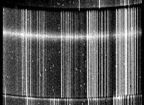
Figure 1: Upper part of a raw FORS1 MOS frame with 3000 seconds exposure time showing the region of slit #2. Wavelength is increasing parallel to the X axis from left to right. A relatively bright ($R=19.94^{m}$) galaxy spectrum is overlaying the night sky emission lines. Note that the magnification scale is larger along the Y axis to demonstrate the distortions by the focal reducer in this direction.

The night sky emission was fitted column by column with first order fits, unless a galaxy spectrum was located at the extreme edges of the slit. In those cases, zero order fits yielded the best results. Night sky subtraction was performed individually for each mask exposure. Prior to the final addition of the three exposures, the optical center of each galaxy along the Y axis has been determined by fitting a Gaussian. If necessary, the spectra were shifted by integer values (two pixels at maximum in a few cases) to ensure consistent profile centers to within at least half a pixel, corresponding to 0.1″. A weighted addition was used if the average seeing varied by more than $\sim$ 20 percent between the exposures.

4 Rotation velocity derivation

4.1 Redshift distribution

Out of the 129 galaxies of which spectra were taken, redshifts could be determined for 113 spirals, including three cases of secondary objects which were covered by a MOS slit by chance. The 16 galaxies without spectroscopic redshifts populate the extreme faint end of our apparent brightness distribution with a median of $\langle R\rangle=22.9^{m}$. Since only one of these spirals features colors of a very late–type SED, the S/N of the remainders may be just too low to yield detectable emission lines. According to the photometric redshifts, the [O II] 3727 doublet is possibly redshifted out of the wavelength range of the R600 grism in the case of 8 targets, while for 5 other galaxies in the regime $0.2<z_{\rm phot}<0.5$, only [O III] or H$\beta$ emission is potentielly covered, which is weaker than H$\alpha$ or [O II] for typical spirals.

Fig. 2 shows the redshift distribution of our sample, restricted to objects with appropriate rotation curves for the TF analysis, see Sect. 4.4 for the constraints. The median redshift is $\langle z\rangle=0.45$. It is likely that the bimodal shape is a combination of the two following effects.

Firstly, as has been outlined in Heidt et al. (Hei03 (2003)), the southwestern corner of the FDF covers the outskirts of a galaxy cluster at $z=0.33$. Allowing a spread in redshift of $\Delta z=0.01$, we find that a maximum of 8 galaxies in our sample could be members of this cluster. The small redshift “bump” at $z\approx 0.3$ can be attributed to these objects.

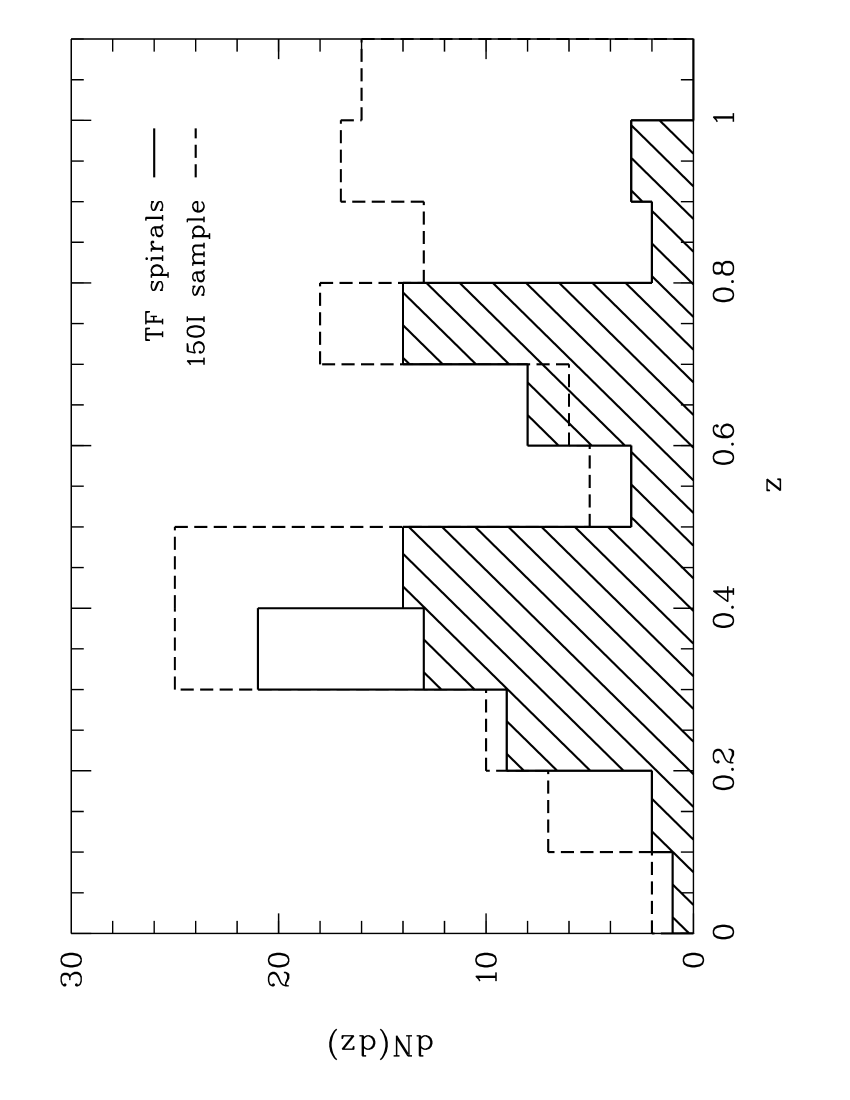
Figure 2: Redshift distribution of the 77 FDF spirals with usable rotation curves (thick solid line). The shaded region gives the distribution after exclusion of 8 possible members of a cluster at $z=0.33$. The dashed line represents the lower resolution spectroscopy sample observed with grism 150I as part of the FDF high–z study (Noll et al. No03 (2004)). Both data sets feature a redshift “gap” around $z\approx$ 0.6, see text for details.

Secondly, the sample contains relatively few galaxies around redshift $z\approx 0.6$. For comparison, we also show the distribution of 144 galaxies at $z<1.1$ from the FDF high–$z$ campaign (Mehlert et al. Me02 (2002), Noll et al. No03 (2004)) which are not contained in our sample. The high–$z$ spectra were taken with the same instrument configuration as the TF data, except that the low–resolution grism 150I was used which covers a much broader wavelength range of $\sim$ 6000 Å in observer’s frame. The large number of galaxies with $z\leq 1$ which did not enter our TF survey can be attributed to the much fainter brightness limits of the high–$z$ study ($I\leq 24.5^{m}$), the inclusion of elliptical galaxies and the lack of constraints to the inclinations. It is clear from Fig. 2 that both samples feature the same redshift “gap”.

As a test, we verified our selection criteria on the most recent version of the FDF photometric redshifts catalogue, finding that only a handfull of types later than Sa could have been missed by the original selection. We therefore conclude that the volume probed with the FDF probably contains fewer galaxies at $z\approx 0.6$ than the neighbouring redshift bins and that the distribution of the TF spirals is unlikely to reflect a selection bias or an observational effect.

4.2 Spectrophotometric classification

To gain a classification of our spectra, three criteria were used. The SED model parameter from the photometric redshifts catalogue, which is related to the star formation e–folding time of the fitted templates, can be transformed into the de Vaucouleurs scheme (ranging from $T=1$ for Sa to $T=10$ for Im). This is useful especially for spectra with very few identifiable lines and/or low S/N, but has the disadvantage that dust reddening might induce a classification of too early a type for highly inclined spirals.

We therefore also performed a comparison to the SED templates in the Kennicutt catalogue (1992a ) with a focus on the relative line strengths of the H$\beta$/[O III] emission. As a third indicator, the rest–frame [O II] 3727 equivalent widths were derived and correlated to type with the values for local spirals given by Kennicutt (1992b ) as a reference.

A combination of these three criteria yielded 14 spirals of type $T\leq 3$ in the redshift range $0.11\leavevmode\nobreak\ \leq\leavevmode\nobreak\ z\leavevmode\nobreak\ \leq\leavevmode\nobreak\ 0.89$ with a median of $\langle z\rangle=0.42$, 43 galaxies with $T=5$ covering $0.09\leavevmode\nobreak\ \leq\leavevmode\nobreak\ z\leavevmode\nobreak\ \leq\leavevmode\nobreak\ 0.97$ with $\langle z\rangle=0.45$ and 20 objects with $T\geq 8$ in the regime $0.23\leavevmode\nobreak\ \leq\leavevmode\nobreak\ z\leavevmode\nobreak\ \leq\leavevmode\nobreak\ 0.97$ with $\langle z\rangle=0.51$.

4.3 Rotation curve extraction

The measurements of the rotation velocity as a function of radius were performed in a semi–automatic manner. In the first step, 100 columns of the spectrum centered on the considered emission line were averaged to get a profile of line plus continuum along the spatial axis. This profile was approximated with a Gaussian to derive the optical center to within 0.1″. For a few objects located very close to the slit edge, the center had to be redefined manually. Then, the emission lines were fitted row by row. To enhance the S/N, three neighbouring rows were averaged prior to the emission line fitting; for very weak lines, this “boxcar” was enlarged to five rows (corresponding to one arcsec). In the case of the [O II] 3727 doublet, two Gaussians with equal FWHM and an observer’s frame separation of $2.75\,(1+z)$ [Å] were assumed as a line profile approximation, while a single Gaussian was used for [O III] 5007, $H\beta$ or $H\alpha$, with the latter being visible only in four spectra. The red- and blueshifts along the spectral axis due to rotation were measured relative to the observed wavelength of the line at the optical center and converted into velocity shifts after cosmological correction by a factor of $(1+z)^{-1}$. This position–velocity information defines an observed  rotation curve (RC).

Each curve was visually inspected prior to the RC modelling. Seven objects had too low a S/N to derive spatially resolved rotation velocities. We also rejected RCs with strong asymmetries or other signatures of substantial kinematic disturbances, “solid–body” rotators and objects that did not show any rotation at all within the measurement errors. In total, the RCs of 77 spirals were appropriate for the $V_{\rm max}$ derivation. We present a range of examples in Fig. 3.

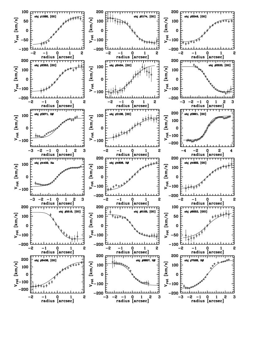
Figure 3: Examples of rotation curves from our data. Observed rotation velocity is plotted against the projected distance from galaxy center. Error bars denote the errors of the Gaussian fits to the emission lines. Object numbers and emission lines used are given for each spiral (either [O II] 3727, [O III] 5007, H$\alpha$ or H$\beta$). The observed rotation curves have been modelled with synthetic velocity fields (solid lines) which take into account geometric distortions due to inclination and slit misalignment as well as seeing and optical beam smearing, see Sect. 4.4 for details. The small spatial extent of the curve of galaxy #5515 to the left hand side is due to contaminating light from a foreground elliptical.

4.4 Rotation curve modelling

For distant, apparently small galaxies, the effect of the slit width on the observed rotation velocity as a function of radius, $V_{\rm rot}^{\rm obs}(r)$, must be considered. At redshift $z=0.5$, a scale length of 3 kpc — typical for an $L^{\ast}$ spiral — corresponds to approx. 0.5 arcsec only, which is half the slit width used in our MOS observations. Any value of $V_{\rm rot}^{\rm obs}(r)$ is therefore an integration perpendicular to the spatial axis (slit direction), a phenomenon which is the optical equivalent to “beam smearing” in radio observations. If not taken into account, this effect could lead to an underestimation of the intrinsic rotation velocities.

We overcame this problem by generating synthetic RCs. Our approach is similiar to the procedure described by Simard & Pritchet (SP99 (1999)) but differs from their fitting method in some ways. E.g., the scale length of the emitting gas is a fixed parameter in our algorithm (see below), and the deviation angle between apparent disk major axis and slit direction is taken into account. Moreover, in our approach we do not fit simulated 2D spectra to observed 2D spectra but simulated RCs to observed RCs.

For the simulation, one has to assume an intrinsic  rotational law $V_{\rm rot}^{\rm int}(r)$. As a first of three variants, we used a simple shape with a linear rise of $V_{\rm rot}^{\rm int}$ at small radii, turning over into a region of constant rotation velocity where the Dark Matter Halo dominates the mass distribution. This can be achieved with the parameterisation

$$V_{\rm rot}^{\rm int}(r)=\frac{V_{\rm max}\,r}{(r^{a}+r^{a}_{0})^{1/a}}$$ (1)

(e.g. Courteau Cou97 (1997)) with a factor $a$ that tunes the sharpness of the “turnover” at radius $r=r_{\rm 0}$, and a constant rotation $V_{\rm rot}^{\rm int}(r)=V_{\rm max}$ for $r\gg r_{\rm 0}$. We used a range of values for $a$ on a set of $\sim$ 20 RCs and found that $a=5$ best reproduced the observed shape of the turnover region. To minimize the number of free parameters, we kept $a$ fixed to that value for all objects in the further analysis. However, due to the heavy blurring of the curves, $a$ is the least critical parameter in Eq. 1.

The turnover radius $r_{\rm 0}$ was assumed to be equal to the scale length of the emitting gas, which is larger than the scale length $r_{\rm d}$ derived from continuum emission. This is discussed in Ryder & Dopita (RD94 (1994)) and Dopita & Ryder (DR94 (1994)) using observational and theoretical approaches, respectively. Since the structural parameters like the continuum scale lengths were measured in an $I$-band VLT image (see Sect. 5.1), we derived the corresponding gas scale length via

$$r_{0}=(2-z/2)\,r_{\rm d}.$$ (2)

This equation yields $r_{0}\approx 2\,r_{\rm d}$ for the least distant FDF spirals (for which $I$ corresponds to rest–frame $R$) and $r_{0}=1.5\,r_{\rm d}$ at $z=1$, where $I$ corresponds to rest–frame $B$. In other words, Eq. 2 is used to gain a correlation between rest–frame scale length and gas scale length that is in compliance with the results of Ryder & Dopita. We also tested this equation directly on a few high S/N emission line profiles in our spectra. It should be noted however, that the $V_{\rm max}$ derivation is much less sensitive to the scale length than to the inclination and the misalignment angle. This is mainly due to the smoothing by the instrumental PSF.

We alternatively used two other templates of intrinsic RC shapes within the Universal Rotation Curve (URC) framework of Persic & Salucci (PS91 (1991), cited as the URC91 hereafter) and Persic et al. (PS96 (1996), URC96 hereafter). The authors introduced a dependence of the RC morphology on luminosity: Only $L^{\ast}$ spirals have a constant $V_{\rm rot}$ at large radii, whereas the curves of sub–$L^{\ast}$ galaxies are rising even beyond a characteristic radius, and very luminous objects have a negative gradient at large radii. The characteristic radii which define a characteristic rotation velocity that can be used for the TF analysis differ slightly between the two approaches. In the URC91 form, this radius is equal to 2.2 scale lengths, whereas it is as large as 3.2 $r_{\rm d}$ for the URC96. Throughout the following sections, the quantity $V_{\rm max}$ will refer to the usage of equation 1, whereas $V_{2.2}$ and $V_{\rm opt}$ denote an input of the URC91 and URC96, respectively.

In the next step of the simulation, the two–dimensional velocity field was generated on the basis of the respective intrinsic rotational law (e.g. Eq. 1 & 2), tilted and rotated according to the observed inclination and position angle of the respective galaxy. The field was then weighted by the normalized surface brightness profile, i.e. brighter regions contribute stronger to the velocity shift at a given radius. Following this, the field was convolved. The Point Spread Function was assumed to be Gaussian with a FWHM determined from the mean DIMM values during the spectroscopy. These values had to be slightly increased depending on the redshifted wavelength of the emission line from which the observed RC was derived. We determined the correlations for this increase by measuring the FWHM on sets of VLT exposures in $B$, $R$, $I$, and comparing these to the according DIMM values. After the double folding, a strip of one arcsecond width was extracted from the velocity field at an angle that matched the slit misalignment in the observation (see Fig. 4). The final computation step was an integration perpendicular to the simulated slit, i.e. the projection of the velocity field strip onto the spatial axis. In all of the following, we will refer to this resulting position–velocity model as the synthetic rotation curve, whereas the rotational law (e.g. Eq. 1) that is used as input for the modelling procedure will be referred to by the term intrinsic rotation curve. The observed RC as described in Sect. 4.3 would directly reproduce the intrinsic RC only for a disk of 90^∘ inclination (i.e., perfectly edge–on) that is observed with an infinitely thin slit at infinitely large spatial and spectral resolution.

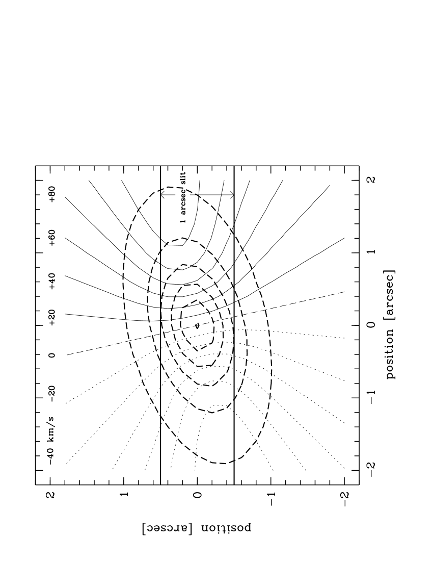
Figure 4: Simulated velocity field for galaxy #4922 inclined by $i$ = 64^∘ with an intrinsic rotation curve of $V_{\rm max}$ = 156 km/s. Thin solid and dotted lines indicate iso–velocity zones ranging from $+120$ km/s to $-120$ km/s rotation in line–of–sight, i.e. comprising a factor $\sin i$. The thick solid lines denote the slit, thick dashed lines sketch the isophotes of the galaxy, with the outermost corresponding to 2$\sigma$ sky noise level in the 3000 s reference $I$-band image (see Sect. 5.1). The misalignment between slit and apparent major axis is $\delta$ = 13^∘.

In our approach, the intrinsic quantity $V_{\rm max}$ is the only free parameter that tunes the reproduction of an observed RC by a synthetic curve. Only in the case of 3 spirals, the gas scale length had to be kept as a second free parameter, since the values based on Eq. 2 were too large. For the complete data set, we derived $V_{\rm max}$ by a visual comparison of synthetic and observed RC and, alternatively, via a $\chi^{2}$-fitting procedure based on the errors from the RC extraction. These two methods are compared in Fig. 5. The sample of 77 spirals is subdivided according data quality: Curves which clearly probe the region of constant rotation velocity at large radii are considered high quality ($N_{\rm obj}=36$), whereas RCs with smaller extent or asymmetries are included in the low quality sub–sample ($N_{\rm obj}=41$).

The error on $V_{\rm max}$ is assumed to be

$$\sigma_{V_{\rm max}}^{2}=\sigma_{\chi^{2}}^{2}+V_{\rm max}^{2}\,(\tan i)^{-2}\,\sigma_{i}^{2}+V_{\rm max}^{2}\,(\tan\delta)^{2}\,\sigma_{\delta}^{2}$$ (3)

Here, the first term on the right hand side is the error from the $\chi^{2}$-fits of the synthetic to the observed RCs, covering the range 3 km/s $\leq\sigma_{\chi^{2}}\leq$ 59 km/s. The last two terms are the propagated errors of the respective uncertainties of the inclination and the misalignment angle. To derive the contributions of the errors $\sigma_{i}$ and $\sigma_{\delta}$, we used a simple geometric correlation between the observed and intrinsic rotation velocity,

$$V^{\rm int}_{\rm rot}=V^{\rm obs}_{\rm rot}\,(\sin i)^{-1}\,(\cos\delta)^{-1}.$$ (4)

For the high quality sample, the absolute and relative errors on $V_{\rm max}$ fall in the respective ranges 3 km/s $\leq\leavevmode\nobreak\ \sigma_{V_{\rm max}}\leavevmode\nobreak\ \leq$ 135 km/s and $0.03\leq\sigma_{V_{\rm max}}/V_{\rm max}\leq 0.61$, with a median $\langle\sigma_{V_{\rm max}}/V_{\rm max}\rangle\leavevmode\nobreak\ =\leavevmode\nobreak\ 0.19$.

As can be deduced from Fig. 5, the by–eye “fits” and the $\chi^{2}$-fits are consistent within the errors for the majority of the objects. Nevertheless, a systematic trend towards low values of $V_{\rm max,\chi^{2}}$ with respect to the visually derived $V_{\rm max,vis}$ is evident for slow rotators. An inspection of the observed RCs revealed that the discrepancies mainly arise in cases of asymmetric shapes. The $\chi^{2}$-fits also are weighted towards the inner parts of the curves by the higher S/N of the emission lines at smaller radii. This is a disadvantage since the outer parts of an observed RC are the most robust source of $V_{\rm max}$ in the modelling procedure. Moreover, we found no correlation between the reduced $\chi^{2}$ values and our definition of RC quality, except for curves of perfect symmetry. For these reasons, we used the visually derived values for the TF analysis. A further discussion of this topic will follow in Sect. 8.3.

In cases of multiple usable emission features in a spectrum, the RCs based on different lines were mostly consistent within the errors. For these objects, $V_{\rm max}$ was derived from the curve with the largest covered radius and highest S/N.

We show a consistency check of the three alternatives for the intrinsic RC shape in Figs. 6 and 7. The results using the simple “rise–turnover–flat” shape via Eq. 1 are in agreement with the URC91 to within 5% for 79% of the FDF spirals and to within 10% for 95% of the galaxies, without a detectable dependence on the absolute values. The URC96 yields rotation velocities at $R_{\rm opt}\approx 3.2\,r_{\rm d}$ which on the mean are larger by 7% than $V_{\rm max}$, with slightly increasing differences towards slow rotation. This partly is an effect of the different characteristic radii in the two parameterisations of the universal rotation curve, which correspond to 2.2 $r_{\rm d}$ for the URC91 and $3.2\,r_{\rm d}$ for the URC96, respectively. However, the slight differences between $V_{\rm max}$ and $V_{\rm opt}$ do not affect the results from our TF analysis, see Sect. 8.3.

Figure 5: Comparison between the $V_{\rm max}$ derivation by visual alignment of observed and synthetic rotation curves (x axis) and via $\chi^{2}$-fits (y axis). Typical error bars are shown for two objects.

Figure 6: Comparison between rotation curve fitting with a simple “rise–turnover–flat” shape (y axis) and the universal rotation curve shape as introduced by Persic & Salucci (PS91 (1991), x axis). Solid symbols denote high quality curves which cover the region of constant rotation velocity at large radii. Typical error bars are shown for two objects.

Figure 7: Comparison between rotation curve fitting with a simple “rise–turnover–flat” shape (y axis) and the universal rotation curve shape as introduced by Persic et al. (PS96 (1996), x axis). High quality curves (solid symbols) cover the region of constant rotation velocity at large radii. Typical error bars are shown for two objects.

5 Photometry

5.1 Luminosity profiles

Since the FDF imaging had been done under varying seeing conditions (ranging, e.g., from 0.46″ to 0.89″ FWHM in the $I$-band, see Heidt et al. Hei03 (2003) for a description of the image stacking), only a limited number of images was used for the measurements of the structural parameters. To combine high spatial resolution with sufficient S/N at the outer isophotes of the TF objects, the 10 $I$-band frames with the best seeing were co–added. This yielded a reference image with 3000 s total exposure time, 0.49″ FWHM and a 50% completeness limit of $\sim$ 25.1^m.

The disk light distributions were fitted with exponential profiles. A bulge component could not be accounted for at the given resolution. We considered slight variations of the PSF across the reference frame with six stars in the range $18<I<20$. Our algorithm minimizes $\chi^{2}$ in the parameter space span by inclination, position angle, scale length and central flux. The sample galaxies cover a range of $25^{\circ}\leq i\leq 80^{\circ}$ with a median of $\langle i\rangle=53^{\circ}$ and a median error of $\langle\sigma_{i}\rangle=5^{\circ}$.

As a test of the accuracy of our ground–based luminosity profile analysis, we also performed measurements on a “VLT simulation” of the Hubble Deep Field North (HDF-N, Williams et al. Wi96 (1996)). The original drizzled images were re–binned to a scale of 0.2″ per pixel and convolved with a Gaussian PSF of 0.49″ FWHM to match the characteristics of our reference $I$-band frame. We selected 40 objects with a variety of $B/T$ ratios and $i>30^{\circ}$ from the electronically available data published by Marleau & Simard (MS98 (1998)). The authors did apply two–component fits to more than 500 galaxies in the HDF-N using the GIM2D package (Galaxy Image Two–Dimensional, Simard et al. Sim02 (2002)). We found that for $B/T<0.4$, the mean difference between the inclinations derived from the “VLT simulation” frame and the original GIM2D values was $\Delta i=1.8^{\circ}\pm 7.7^{\circ}$.

The median inclinations of our TF sample sub–divided according to SED type are $\langle i\rangle=51^{\circ}$ for $T\leq 3$, $\langle i\rangle=53^{\circ}$ for $T=5$ and $\langle i\rangle=51^{\circ}$ for $T=8$, i.e. potentially unresolved bulge components of early–type spirals in our ground–based imaging did not introduce a detectable bias.

5.2 Rest–frame magnitudes

Total apparent magnitudes were derived with the Source Extractor package (Bertin & Arnouts BA96 (1996)). This program offers different algorithms for the photometry. We used the Mag_auto routine with variable elliptical apertures which is based on the “first moment” algorithm by Kron (Kro80 (1980)) since it best reproduces the total magnitudes of extended sources.

We will now briefly discuss the issue of the $k$-correction. If available broad band information is limited to a few filters (in most previous studies two or even only one), the different wavelength ranges covered by a passband in observed frame and rest–frame introduce a strong dependence of the possible $k$-correction accuracy on SED type. At redshift $z=0.6$, e.g., the difference between $T=4$ and $T=6$ corresponds to a change of half a magnitude in the transformation from $B_{\rm obs}$ to $B_{\rm rest}$, $k_{B}$ (e.g. Frei & Gunn FG94 (1994)). Values of $k_{B}$ differ even more for earlier types, thus even a slight misclassification can introduce a substantial offset in the derived luminosity if observations are limited to one or two filters. In contrast to this, our TF project greatly benefits from the multi–band imaging of the FDF: The photometry in $B$, $g$, $R$ and $I$ enables us to use the filter that best matches the rest–frame $B$-band to transform an apparent magnitude $X$ into absolute magnitudes $M_{B}$ up to the highest redshifts in the sample.

We computed the $k_{B}$-correction for our objects via synthetic photometry on SEDs in the range $1\leq T\leq 10$. As templates, we used the spectra published by Möller et al. (Moe01 (2001)) which were generated with evolutionary synthesis models. The SEDs were redshifted by re–calculating the original flux $F_{0}$ at wavelength $\lambda$ according to

$$F(\lambda,z)=\frac{F_{0}[\lambda/(1+z)]}{(1+z)}$$ (5)

(e.g. Contardo, Steinmetz & Fritze-v. Alvensleben CSF98 (1998)). Transformation from the apparent magnitude of a spectrum of type $T$ at redshift $z$ observed with a FORS filter $X$ to the un–redshifted spectrum in Johnson $B$ yields $k_{B}(X,T,z)$. Respective filters used for the input magnitudes were $B_{\rm FORS}$ for $z<0.25$, $g_{\rm FORS}$ for $0.25\leq z<0.55$, $R_{\rm FORS}$ for $0.55\leq z<0.85$ and $I_{\rm FORS}$ for $z\geq 0.85$. This $k$-correction is much less sensitive to spectral type than a transformation $B_{\rm obs}\rightarrow B_{\rm rest}$, especially at higher redshifts: e.g., $k_{B}(R,1,0.6)-k_{B}(R,5,0.6)=0.05^{m}$ whereas $k_{B}(B,1,0.6)-k_{B}(B,5,0.6)=0.64^{m}$.

For testing purposes, we additionally derived the colors of the templates purely within the Johnson-Cousins Filter system and compared them to the values published by Fukugita et al. (Fuk95 (1995)), finding typical absolute deviations of $0.03^{m}\leavevmode\nobreak\ \leq\leavevmode\nobreak\ |\Delta(X\leavevmode\nobreak\ -\leavevmode\nobreak\ Y)|\leavevmode\nobreak\ \leq\leavevmode\nobreak\ 0.08^{m}$.

The second critical correction that has to be applied to the observed magnitudes is the inclination–dependent intrinsic absorption $A_{B}^{i}$ by the dust disks of the objects. Like, e.g., Vogt et al. (Vog96 (1996), Vog97 (1997)) and Milvang-Jensen et al. (Mil03 (2003)), we adopted the approach by Tully & Fouqué (TF85 (1985)). It is based on geometric assumptions and usable for inclinations up to $i=80^{\circ}$, i.e. for our complete sample. The dust disk scale height is assumed to be half the scale height of the luminous disk, relative dust content is independent of mass or type, with an optical depth of $\tau=0.55$. For the objects in our sample, $A_{B}^{i}$ spans values from 0.30^m at $i=25^{\circ}$ to 0.96^m at $i=80^{\circ}$. We emphasize that the absorption for face–on disks is finite in this convention: $A_{B}^{i}=0.27^{m}$ for $i=0^{\circ}$. Our multi–band photometry ensures to compute the absorption for the same rest–frame wavelength interval at all the covered redshifts.

For the galactic absorption at the coordinates of the FDF, we adopted the values which are given in Heidt et al. (Hei03 (2003)), ranging from $A_{B}^{g}=0.076^{m}$ to $A_{I}^{g}=0.035^{m}$. Let $D_{\Lambda}(z,H_{0})$ be the distance modulus (e.g. Peebles Pe93 (1993)) in the concordance cosmology, then the transformation from total apparent magnitude $m_{X}$ to absolute magnitude $M_{B}$ is given by

$$M_{B}=m_{X}-D_{\Lambda}(z,H_{0})-k_{B}(X,T,z)-A_{B}^{i}-A_{X}^{g}$$ (6)

If one assumes an SED classification error of $\Delta T=2$ (i.e., an Sc spiral could be misclassified as an Sb and vice versa), corresponding to an uncertainty of the $k$-correction of $\sigma_{k}\leavevmode\nobreak\ \leq\leavevmode\nobreak\ 0.1^{m}$ for all covered types and redshifts, the errors in absolute magnitude become

$$\sigma_{M_{B}}^{2}=\sigma_{X}^{2}+\sigma_{k}^{2}+\sigma_{A_{B}^{i}}^{2},$$ (7)

where $\sigma_{X}$ is the random photometric error in the respective filter and $\sigma_{A_{B}^{i}}$ the uncertainty of the intrinsic absorption correction via error propagation from the inclination error. Thanks to the very deep imaging, the random photometric errors are only $0.01^{m}$ on average and $0.03^{m}$ at maximum for the FDF spirals. Based on a comparison of our calibrations with archived FORS zero points, we estimate the systematic photometric errors to be $\leq 0.01^{m}$; these are neglected. The total errors $\sigma_{M_{B}}$ of our complete sample fall into the range $0.07^{m}\leq\sigma_{M_{B}}\leq 0.21^{m}$.

6 The data table

We present the data of the spirals from our sample in Table 1. This table is available in electronic form via anonymous ftp to cdsarc.u-strasbg.fr. The respective columns have the following meaning:

ID — Original entry number from the FORS Deep Field photometric catalogue, see Heidt et al. (Hei03 (2003)) for, e.g., the J2000 positions or aperture magnitudes in $U$, $B$, $g$, $R$, $I$, $J$ and $K$.

Table 1: The data of the 77 spirals from the FORS Deep Field Tully–Fisher sample.

ID	$i$	$\delta$	$r_{\rm d}$	$z$	$T$	$X$	$k_{B}$	$A^{g}_{X}$	$A^{i}_{B}$	$D_{\Lambda}$	$M_{B}$	$V_{\rm max}\hskip 6.5pt$	$B$$-$$R$	note
	[deg]	[deg]	[ ′′]			[mag]	[mag]	[mag]	[mag]	[mag]	[mag]	[km/s]	[mag]
400	60	23	0.70	0.4483	10	22.63	$+$0.25	0.06	0.49	41.98	$-$20.15$\pm$0.13	74$\pm$19	0.21	L
745	42	61	0.49	0.6986	5	21.06	$-$0.49	0.04	0.35	43.14	$-$21.98$\pm$0.08	402$\pm$167	1.00	L
870	53	8	0.53	0.2775	5	20.77	$-$0.07	0.06	0.42	40.76	$-$20.40$\pm$0.08	96$\pm$6	0.73	H
1082	49	10	0.50	0.4482	8	22.14	$+$0.36	0.06	0.39	41.98	$-$20.66$\pm$0.08	118$\pm$16	0.75	H
1224	49	5	0.34	0.3989	10	23.26	$+$0.16	0.06	0.39	41.68	$-$19.03$\pm$0.13	43$\pm$16	0.26	L
1327	31	1	0.62	0.3141	3	20.50	$+$0.11	0.06	0.31	41.07	$-$21.05$\pm$0.07	204$\pm$36	0.91	L
1449	36	30	0.66	0.1140	5	20.52	$+$0.40	0.08	0.33	38.62	$-$18.90$\pm$0.08	51$\pm$16	0.67	L
1476	77	10	0.80	0.4360	3	22.72	$+$0.47	0.06	0.85	41.91	$-$20.58$\pm$0.09	283$\pm$26	1.52	L
1569	37	3	0.34	0.4625	8	24.16	$+$0.39	0.06	0.33	42.06	$-$18.69$\pm$0.13	57$\pm$50	0.69	L
1625	57	10	0.38	0.2304	5	23.37	$+$0.74	0.08	0.46	40.30	$-$18.20$\pm$0.09	122$\pm$42	0.84	L
1655	51	0	0.49	0.3377	5	21.88	$+$0.12	0.06	0.41	41.25	$-$19.96$\pm$0.08	126$\pm$8	0.84	L
1699	48	11	0.21	0.2299	8	22.67	$+$0.68	0.08	0.38	40.30	$-$18.77$\pm$0.13	55$\pm$15	0.11	L
1834	49	7	0.25	0.3475	5	24.06	$+$0.15	0.06	0.39	41.33	$-$17.88$\pm$0.13	62$\pm$37	1.39	L
1928	60	12	0.29	0.7179	10	22.89	$-$0.46	0.04	0.49	43.22	$-$20.40$\pm$0.13	105$\pm$29	0.42	L
2007	62	5	0.40	0.7175	10	22.68	$-$0.46	0.04	0.52	43.21	$-$20.63$\pm$0.11	84$\pm$20	0.48	L
2067	35	19	0.40	0.7942	5	21.87	$-$0.32	0.04	0.32	43.48	$-$21.65$\pm$0.08	210$\pm$58	0.97	H
2174	57	5	0.43	0.6798	3	22.08	$-$0.49	0.04	0.46	43.07	$-$21.00$\pm$0.09	175$\pm$24	1.21	H
2246	45	0	0.60	0.6514	5	21.52	$-$0.58	0.04	0.37	42.96	$-$21.27$\pm$0.09	183$\pm$29	1.03	H
2328	68	10	0.50	0.3956	8	22.44	$+$0.26	0.06	0.61	41.66	$-$20.16$\pm$0.11	150$\pm$18	0.78	L
2341	32	5	0.35	0.7611	5	22.09	$-$0.38	0.04	0.31	43.37	$-$21.25$\pm$0.09	279$\pm$107	1.07	H
2353	41	9	0.50	0.7773	3	22.05	$-$0.29	0.04	0.35	43.43	$-$21.48$\pm$0.09	209$\pm$44	1.21	H
2397	40	25	0.80	0.4519	5	21.98	$+$0.42	0.06	0.34	42.00	$-$20.84$\pm$0.08	98$\pm$22	0.71	H
2484	52	15	0.52	0.6535	5	21.78	$-$0.58	0.04	0.41	42.97	$-$21.07$\pm$0.09	169$\pm$36	1.10	H
2533	65	34	0.90	0.3150	5	20.42	$+$0.04	0.06	0.56	41.08	$-$21.32$\pm$0.09	230$\pm$16	0.99	H
2572	56	8	0.38	0.4491	5	23.00	$+$0.41	0.06	0.45	41.98	$-$19.90$\pm$0.10	74$\pm$19	0.86	H
2574	68	14	0.45	0.6802	5	22.98	$-$0.53	0.04	0.61	43.07	$-$20.22$\pm$0.13	162$\pm$29	0.95	L
2783	42	3	0.52	0.3143	5	21.57	$+$0.04	0.06	0.35	41.07	$-$19.95$\pm$0.08	84$\pm$17	0.83	L
2800	47	4	0.61	0.6290	8	22.23	$-$0.64	0.04	0.38	42.87	$-$20.42$\pm$0.09	143$\pm$27	0.86	H
2822	52	5	0.35	0.5871	8	21.80	$-$0.71	0.04	0.41	42.68	$-$20.62$\pm$0.09	107$\pm$21	0.85	L
2946	56	15	0.28	0.7437	10	22.99	$-$0.42	0.04	0.45	43.31	$-$20.38$\pm$0.13	108$\pm$34	0.35	L
2958	55	15	0.82	0.3139	5	21.48	$+$0.04	0.06	0.44	41.07	$-$20.13$\pm$0.08	141$\pm$13	0.73	H
3071	38	35	0.55	0.0939	5	19.53	$+$0.34	0.08	0.34	38.17	$-$19.39$\pm$0.08	176$\pm$20	0.83	H
3108	61	3	0.62	0.4741	5	23.33	$+$0.46	0.06	0.50	42.12	$-$19.81$\pm$0.11	104$\pm$26	1.01	H
3131	54	3	0.37	0.7723	5	22.47	$-$0.36	0.04	0.43	43.41	$-$21.05$\pm$0.12	166$\pm$26	0.92	L
3578	61	3	0.56	0.7718	5	22.68	$-$0.36	0.04	0.50	43.41	$-$20.91$\pm$0.13	154$\pm$37	1.06	H
3704	80	6	0.48	0.4082	3	23.92	$+$0.42	0.06	0.96	41.74	$-$19.27$\pm$0.16	40$\pm$20	1.27	L
3730	68	2	0.45	0.9593	5	22.97	$-$0.95	0.04	0.61	43.99	$-$20.72$\pm$0.15	156$\pm$41	0.73	H
3921	59	12	1.42	0.2251	3	19.90	$+$0.82	0.08	0.48	40.25	$-$21.73$\pm$0.11	245$\pm$19	1.01	H
4113	69	2	0.48	0.3951	1	23.04	$+$0.46	0.06	0.63	41.65	$-$19.77$\pm$0.12	249$\pm$53	1.12	L
4371	25	39	0.30	0.4605	3	23.13	$+$0.52	0.06	0.30	42.05	$-$19.80$\pm$0.09	361$\pm$330	1.16	L
4376	71	1	0.42	0.3961	8	23.72	$+$0.27	0.06	0.67	41.66	$-$18.94$\pm$0.11	74$\pm$18	0.62	L
4402	75	9	1.57	0.1138	3	20.24	$+$0.47	0.08	0.78	38.62	$-$19.71$\pm$0.09	95$\pm$3	0.75	H
4465	61	9	0.40	0.6117	5	21.56	$-$0.65	0.04	0.50	42.79	$-$21.12$\pm$0.10	170$\pm$26	1.04	L
4498	40	40	0.33	0.7827	8	22.60	$-$0.38	0.04	0.34	43.45	$-$20.85$\pm$0.11	95$\pm$58	0.82	L
4657	37	5	0.70	0.2248	5	21.79	$+$0.73	0.08	0.33	40.24	$-$19.58$\pm$0.08	212$\pm$14	0.91	H
4730	32	3	0.90	0.7820	1	20.94	$-$0.23	0.04	0.31	43.44	$-$22.63$\pm$0.08	430$\pm$84	1.41	L
4806	65	4	0.70	0.2214	5	22.07	$+$0.72	0.08	0.56	40.21	$-$19.50$\pm$0.08	209$\pm$17	0.72	H
4922	64	13	0.71	0.9731	10	21.77	$-$1.06	0.04	0.54	44.03	$-$21.78$\pm$0.11	156$\pm$27	0.22	H
5022	73	10	0.61	0.3385	10	22.94	$-$0.04	0.06	0.72	41.26	$-$19.06$\pm$0.14	75$\pm$6	0.51	L
5140	50	5	0.60	0.2738	5	22.94	$-$0.08	0.06	0.40	40.73	$-$18.16$\pm$0.10	125$\pm$39	0.85	L
5286	65	1	0.34	0.3337	8	23.88	$+$0.06	0.06	0.56	41.22	$-$18.02$\pm$0.18	23$\pm$7	0.64	L
5317	53	5	0.59	0.9745	5	21.39	$-$0.92	0.04	0.42	44.03	$-$22.18$\pm$0.09	236$\pm$36	0.71	L

Table 1: — continued.

ID	$i$	$\delta$	$r_{\rm d}$	$z$	$T$	$X$	$k_{B}$	$A^{g}_{X}$	$A^{i}_{B}$	$D_{\Lambda}$	$M_{B}$	$V_{\rm max}\hskip 6.5pt$	$B$$-$$R$	note
	[deg]	[deg]	[ ′′]			[mag]	[mag]	[mag]	[mag]	[mag]	[mag]	[km/s]	[mag]
5335	30	10	0.29	0.7726	5	22.53	$-$0.36	0.04	0.31	43.41	$-$20.86$\pm$0.10	220$\pm$135	0.92	H
5361	46	5	0.19	0.3339	5	22.45	$+$0.10	0.06	0.37	41.23	$-$19.32$\pm$0.09	75$\pm$19	1.05	L
5515	49	35	0.39	0.8934	3	21.33	$-$1.03	0.04	0.39	43.80	$-$21.86$\pm$0.10	269$\pm$87	0.81	H
5565	63	8	0.43	0.2285	8	23.55	$+$0.68	0.08	0.53	40.28	$-$18.01$\pm$0.11	41$\pm$10	0.25	L
6125	57	5	0.22	0.4495	5	22.78	$+$0.41	0.06	0.46	41.99	$-$20.14$\pm$0.08	152$\pm$18	1.52	H
6253	76	7	0.61	0.3453	5	23.75	$+$0.14	0.06	0.81	41.31	$-$18.58$\pm$0.19	95$\pm$19	0.69	H
6406	45	0	0.60	0.8451	3	21.65	$-$0.16	0.04	0.37	43.65	$-$22.25$\pm$0.08	250$\pm$36	1.15	H
6452	45	60	0.24	0.3359	5	23.15	$+$0.11	0.06	0.37	41.24	$-$18.63$\pm$0.11	109$\pm$52	0.78	L
6568	53	15	0.46	0.4597	5	22.85	$+$0.43	0.06	0.42	42.04	$-$20.11$\pm$0.09	144$\pm$30	1.06	L
6585	71	8	1.45	0.3357	5	20.26	$+$0.11	0.06	0.67	41.24	$-$21.83$\pm$0.08	295$\pm$7	1.46	H
6657	28	4	0.50	0.3343	3	20.99	$+$0.18	0.06	0.30	41.23	$-$20.78$\pm$0.07	254$\pm$54	1.26	H
6743	39	15	0.33	0.7320	8	22.73	$-$0.47	0.04	0.34	43.27	$-$20.46$\pm$0.10	118$\pm$48	0.77	H
6921	47	13	0.35	0.4538	5	23.47	$+$0.42	0.06	0.38	42.01	$-$19.40$\pm$0.12	111$\pm$46	0.86	H
7298	33	15	0.50	0.3902	5	21.48	$+$0.29	0.06	0.32	41.62	$-$20.81$\pm$0.09	115$\pm$56	0.98	H
7429	55	15	0.40	0.3370	5	21.68	$+$0.11	0.06	0.44	41.25	$-$20.19$\pm$0.09	90$\pm$17	0.73	L
7526	59	5	0.77	0.3589	5	20.86	$+$0.19	0.06	0.48	41.41	$-$21.28$\pm$0.07	181$\pm$7	0.93	H
7597	68	13	0.26	0.4096	5	24.24	$+$0.34	0.06	0.61	41.75	$-$18.52$\pm$0.21	79$\pm$34	0.87	L
7725	62	15	0.49	0.5504	8	22.18	$-$0.77	0.04	0.52	42.51	$-$20.12$\pm$0.12	84$\pm$38	0.86	L
7733	51	10	0.68	0.4471	5	22.79	$+$0.41	0.06	0.41	41.97	$-$20.06$\pm$0.09	89$\pm$17	0.75	H
7856	54	9	0.40	0.5146	5	22.63	$+$0.52	0.06	0.43	42.32	$-$20.69$\pm$0.09	273$\pm$35	1.23	L
7866	53	27	0.30	0.2240	3	23.11	$+$0.82	0.08	0.42	40.23	$-$18.44$\pm$0.10	50$\pm$45	0.97	L
8034	42	0	0.22	0.7317	5	22.34	$-$0.43	0.04	0.35	43.27	$-$20.89$\pm$0.11	173$\pm$49	0.90	H
8190	45	2	0.38	0.3947	5	21.84	$+$0.31	0.06	0.37	41.65	$-$20.55$\pm$0.08	113$\pm$12	0.76	H
8360	63	27	0.52	0.7034	10	22.58	$-$0.48	0.04	0.53	43.16	$-$20.67$\pm$0.16	120$\pm$62	0.46	L
8526	71	12	0.53	0.6095	5	21.90	$-$0.66	0.04	0.67	42.78	$-$20.94$\pm$0.14	135$\pm$10	0.75	L

$i$ — Disk inclination derived by minimizing $\chi^{2}$ of a two–dimensional exponential profile fit to the galaxy image in a coadded $I$-band frame with 0.49 arcsec FWHM (see Sect. 5.1). In some cases, our initial constraint of $i\geq 40^{\circ}$ had to be relaxed.

$\delta$ — Absolute misalignment angle between the MOS slit and the apparent major axis. Our initial constraint of $\delta\leq 15^{\circ}$ could not always be met during the construction of the setups.

$r_{\rm d}$ — Apparent disk scale length in arcseconds, derived via the same fits as $i$ and $\delta$. While tests confirmed that $r_{\rm d}$ is the least critical input parameter in the $V_{\rm max}$ derivation process, it is probably the one which is affected the strongest by the limitations of the ground–based imaging. Hence, we recommend not to use these values for applications like the Fundamental Plane of spiral galaxies.

$z$ — Spectroscopic redshift.

$T$ — SED type in the de Vaucouleurs scheme (see Sect. 4.2 for a description of the classification criteria). $T=1$ accounts to Hubble type Sa, $T=3$ to Sb, $T=5$ to Sc, $T=8$ to Sdm and $T=10$ to Im.

$X$ — Total apparent magnitude derived with the Mag_auto algorithm of the Source Extractor package (Bertin & Arnouts BA96 (1996)) on the coadded FDF frames. Depending on the galaxies redshift, the filter $X$ was chosen to best match the rest–frame $B$-band. For the least redshifted spirals with $z<0.25$, this was $X=B$, for $0.25\leq z<0.55$ we chose $X=g$, for $0.55\leq z<0.85$ we set $X=R$, and for the highest redshifts in our sample with $z\geq 0.85$ we used $X=I$.

$k_{B}$ — K–correction for the transformation from the respective filter $X$ (see above) to rest–frame $B$ as computed via synthetic photometry, see Sect. 5.2 for details.

$A^{g}_{X}$ — Galactic absorption in the respective filter $X$ (see above) as given in Heidt et al. (Hei03 (2003)).

$A^{i}_{B}$ — Intrinsic inclination–dependent dust absorption in rest–frame $B$ following Tully & Fouqué (TF85 (1985)) with the convention of a non–negligible extinction for face–on disks, i.e. $A^{i}_{B}=0.27^{m}$ at $i=0^{\circ}$.

$D_{\Lambda}$ — Distance modulus in concordance cosmology with $\Omega_{\rm m}$ = 0.3, $\Omega_{\Lambda}$ = 0.7 and $H_{0}$ = 70 km s^-1 Mpc^-1.

$M_{B}$ — Absolute $B$-band magnitudes computed via $M_{B}=X-k_{B}-A^{g}_{X}-A^{i}_{B}-D_{\Lambda}$. The errors include the uncertainties in $X$, $k_{B}$ and $A^{i}_{B}$, see Sect. 5.2 for details.

$V_{\rm max}$ — Intrinsic maximum rotation velocity derived via synthetic velocity fields (see Sect. 4) assuming a linear rise of the rotation velocity at small galactocentric radii and a flat RC at large radii (“rise–turnover–flat” shape). The errors on $V_{\rm max}$ were computed according to Eq. 3.

$B$$-$$R$ — Rest–frame color index, corrected for intrinsic absorption. For galaxies with $z<0.25$, apparent $R$ magnitudes were transformed to rest–frame $R$, while apparent $I$ magnitudes were transformed to rest–frame $R$ for all other objects, see Sect. 8.1 for details.

note — Label indicating the RC quality. High quality curves (“H”) extend well out to the region of constant rotation velocity at large radii. RCs of low quality (“L”) have a smaller radial extent and partly feature signatures of moderate kinematic perturbations like waves or asymmetries.

7 The distant $\mathbf{B}$-band Tully–Fisher relation

To be able to derive the spectrophotometric and/or kinematic evolution of spirals at intermediate redshifts, it is crucial to carefully choose a data set of spirals at low $z$ that can be used as reference. Consistency between distant and local data set in terms of the intrinsic absorption correction is one of the key issues. As stated in the introduction, a large number of local samples have been constructed during the last decade, with kinematic data based on radio observations or optical spectra. For our purposes, the term “local” refers to redshifts below $z\leq 0.05$ corresponding to systematic velocities $V_{\rm sys}\leq 15000$ km/s. In Ziegler et al. (Zie02 (2002)), we selected a sample by Haynes et al. (Hay99 (1999)) as a local reference. Here, we will use the data set of Pierce & Tully (PT92 (1992), PT92 hereafter) instead. Our initial choice was basically motivated by the very good statistics of the Haynes et al. sample which comprises approx. 1200 spirals mainly of type Sc, which is also the most frequent SED type in our distant sample.

On the other hand, using the PT92 data makes our results directly comparable to the studies of e.g., Vogt (Vog01 (2001)) and Milvang-Jensen et al. (Mil03 (2003)). Moreover, the TFR of PT92 benefits from the inclusion of spirals with Cepheid–calibrated distances. As for our sample, the photometry has been corrected for dust–reddening via the Tully & Fouqué approach. A difference that has to be accounted for is the convention for face–on extinction (see Sect. 5.2) used by PT92, i.e., an offset of $\Delta M_{B}=0.27^{m}$ has to be applied. This way, the local $B$-band TFR transforms into

$$M_{B}=-7.48\log V_{\rm max}-3.52$$ (8)

with an observed scatter of $\sigma_{B}=0.41^{m}$. This is in good agreement with a bisector fit to the Haynes et al. sample restricted to 1097 galaxies with H I profiles classified as good quality by the authors:

$$M_{B}=-7.85\log V_{\rm max}-2.78.$$ (9)

Here, we transformed apparent $I$-band magnitudes into $B$ via colors from Frei & Gunn (FG94 (1994)). The two TFRs are perfectly consistent in the low–mass regime and show only a small offset of $\Delta M\approx 0.18^{m}$ at $V_{\rm max}=300$ km/s.

In Fig. 8, we show the TF diagram of the complete FDF spiral sample along with the local relation from PT92. As in Sect. 4, our sample is sub–divided according to the RC quality. For the high quality data, the curves have a sufficient spatial extent to probe the region of constant rotation velocity at large radii, thereby yielding robust values of $V_{\rm max}$. In the case of the low quality data, on the other hand, we cannot rule out the possibility that at least for a fraction of the objects $V_{\rm max}$ is underestimated, i.e. offsets from the local TFR towards higher luminosities could be overestimated. For this reason, we will use only the high quality data for the following analysis. These spirals cover the ranges $-18.6^{m}\geq M_{B}\geq-22.2^{m}$ in absolute magnitude and $74\,{\rm km/s}\leq\log V_{\rm max}\leq 295\,{\rm km/s}$ in maximum rotation velocity.

Figure 8: FORS Deep Field sample of spirals in the range $0.1\leq z\leq 1.0$ in comparison to the local TFR by Pierce & Tully (PT92 (1992), dotted lines give 3 $\sigma$ limits). The distant sample is subdivided according to rotation curve quality: High quality curves (solid symbols) extend well out to the region of constant rotation velocity at large radii.

For a given $V_{\rm max}$, the difference in luminosity of an FDF object from the local PT92 fit is given by

$$\Delta M_{B}=7.48\log V_{\rm max}+3.52+M_{B}.$$ (10)

These offsets are shown as a function of redshift in Fig. 9. Although the scatter of the offsets is reduced from $\sigma_{\Delta M}\nobreak=\nobreak 1.32^{m}$ to $\sigma_{\Delta M}\nobreak=\nobreak 0.97^{m}$ when restricting the FDF sample to high quality RCs, this is still over a factor of two larger than for the local data set. We speculate that this partly is an effect of the observational limitations for distant spirals like, e.g., the low intrinsic spatial resolution, but also reflects a broader range of star formation efficiencies than in the local universe. This interpretation is supported by the smaller scatter of the offsets which originates from the uncertainty in $V_{\rm max}$ and amounts to 0.63 mag for the HQ data.

A linear $\chi^{2}$-fit to the high quality data yields

$$\Delta M_{B}=-(1.22\pm 0.56)\cdot z-(0.09\pm 0.24).$$ (11)

For this fit, the error was computed as

$$\sigma^{2}_{\Delta M_{B}}=\sigma^{2}_{M^{\rm FDF}_{B}}+7.48^{2}\sigma^{2}_{\log V^{\rm FDF}_{\rm max}}$$

$$+\sigma^{2}_{M^{\rm PT}_{B}}+7.48^{2}\sigma^{2}_{\log V^{\rm PT}_{\rm max}},$$ (12)

where the second and fourth term are the propagated errors from the uncertainties in $\log V_{\rm max}$ for the FDF spirals and the PT92 sample, respectively.

As can be deduced from Eq. 11, we observe an increasing brightening with rising look–back time. This is expected as an effect of the younger stellar populations, i.e. a higher fraction of high–luminosity stars than in the local universe. Our result is in agreement with those of Barden et al. (Ba03 (2003), $\Delta M_{B}=-1.1\pm 0.5$ at $\langle z\rangle\approx 0.9$) and Milvang-Jensen (Mil03b (2003)), who finds $\Delta M_{B}=-(0.9\pm 0.3)\,\cdot\,z$, note that the latter correlation would be slightly steeper in the cosmology adopted here. A much smaller brightening of less than 0.2 mag at $z\leq 1$ is found by Vogt (Vog01 (2001)).

Figure 9: Offsets of the FORS Deep Field sample from the local TFR as given by Pierce & Tully (PT92 (1992)) as a function of redshift. Filled symbols denote rotation curves which extend well out to the region of constant rotation velocity at large radii (labeled high quality data).

Besides the dependency of $\Delta M_{B}$ on redshift, the comparison of our sample with PT92 in Fig. 8 indicates a correlation between the TF offsets and maximum rotation velocity. Even restricting to rotation curves which probe the “flat” region at large radii, a number of distant spirals in the regime $V_{\rm max}\approx 100$ km/s are overluminous with $>$3 $\sigma$ confidence, given the observed scatter of 0.41 mag for the local sample. This can be seen in Fig. 10, where the offsets are plotted against the logarithm of $V_{\rm max}$. A linear $\chi^{2}$-fit to the high quality subsample with an error estimation as defined in Eq. 7 yields

$$\Delta M_{B}=(4.40\pm 0.69)\log V_{\rm max}-(10.31\pm 1.55),$$ (13)

corresponding to a brightening by more than two magnitudes for the least massive spirals in our sample and negligible offsets at $V_{\rm max}\approx 220$ km/s, which on the basis of Eq. 8 is the typical rotation for local spirals of luminosity 2-3$L^{\ast}$.

Figure 10: Offsets of the FORS Deep Field sample from the local TFR as given by Pierce & Tully (PT92 (1992)) as a function of maximum rotation velocity. We observe large overluminosities for objects with slow rotation (i.e. low mass) and negligible offsets for fast rotators (i.e. high–mass spirals). Filled symbols denote rotation curves which extend well out to the region of constant rotation velocity at large radii (labeled high quality data).

8 Discussion

Before interpreting the possible physical implications of Eq. 13, we want to comment on a potential correlation between the TF offsets and the errors in $V_{\rm max}$. In Fig. 11, the offsets are plotted against the relative errors $\sigma_{V_{\rm max}}$/$V_{\rm max}$. Even if only the galaxies with high quality RCs are considered, the overluminosities seem to be higher for objects with larger $V_{\rm max}$ errors. We see two basic reasons for this slight dependency.

Figure 11: Offsets of the FORS Deep Field sample from the local TFR as given by Pierce & Tully (PT92 (1992)), plotted against the relative errors in $V_{\rm max}$. The weak correlation between these two parameters can attributed to the lower RC quality and the larger relative errors of the RC extraction for slow rotators, see text for details. Filled symbols denote rotation curves which extend well out to the region of constant rotation velocity at large radii.

Firstly, the RC quality on the mean is lower for low–mass objects. In particular, the least massive FDF spirals all are classified as low quality data. A lower rotation curve quality in turn leads to higher values of $\sigma_{\chi^{2}}$ (Eq. 3) and an increased total error of the maximum rotation velocity. And secondly, the errors of the Gaussian fits to the emission lines which are performed in the process of the RC extraction do not depend on the magnitude of the velocity shifts. On the other hand, for a given radius and fit uncertainty, the relative errors on $V_{\rm rot}^{\rm obs}(r)$ are smaller for fast rotators. Since the observed relative errors contribute to the derived value of $\sigma_{\chi^{2}}$, this error is on the mean larger for slow rotators.

The combination of these two effects leads to larger relative errors for small values of $V_{\rm max}$, i.e., for spirals with large TF offsets.

We will now consider potential biases due to galaxy-galaxy interactions or sample incompleteness, the impact of the intrinsic rotation curves shape and the question of different conventions for the intrinsic absorption correction.

8.1 A bias due to environmental effects?

To some extent, a correlation between rotation velocity and TF offsets is to be expected from previous studies. Kannappan et al. (Kan02a (2002)) found a color–residuals relation that reflects overluminosities of blue spirals and argued that this could be attributed to enhanced star formation. Since galaxies with blue colors, i.e. late types, feature on the mean lower values of $V_{\rm max}$ than red, early–type spirals (see Sect. 8.5), a correlation between colors and TF offsets should coincide with a relation between the offsets and $V_{\rm max}$.

To look into this effect, we computed the $B-R$ color index of our FDF galaxies in rest–frame. In contrast to the initial derivation of the absolute magnitudes, we did not use total apparent magnitudes but brightnesses that were measured within apertures of two arcseconds diameter on coadded frames which were convolved to the same seeing (see Heidt et al. Hei03 (2003) for details). Similarly to the procedure for the $B$-band luminosities, we transformed the observed $R_{\rm FORS}$ into $R^{\rm rest}_{\rm Cousins}$ only for low–redshift galaxies ($z<0.25$) and used the transformation $I_{\rm FORS}\rightarrow R^{\rm rest}_{\rm Cousins}$ instead for all objects at larger distances. The absorption coefficients with respect to rest–frame $R$ were computed following Cardelli et al. (Ca89 (1989)) using again the intrinsic absorption convention by Tully & Fouqué (TF85 (1985)).

For the purpose of the color–residual relation, we compare our data to the local sample from Verheijen (2001). We show the offsets with respect to the Verheijen TFR

$$M_{B}=-8.1\log V_{\rm max}-2.07$$ (14)

for our high quality sample in Fig. 12. Only a weak dependence of the offsets on rest–frame color is observed. In contrast to the results for the local spirals, offsets of the FDF spirals almost solely populate the regime of overluminosities with a median of $-0.7^{m}$ and 12 out of 36 galaxies feature offsets of more than one magnitude from the local TFR. Note that this is consistent with the offsets from the PT92 relation which have a median of $-0.77^{m}$.

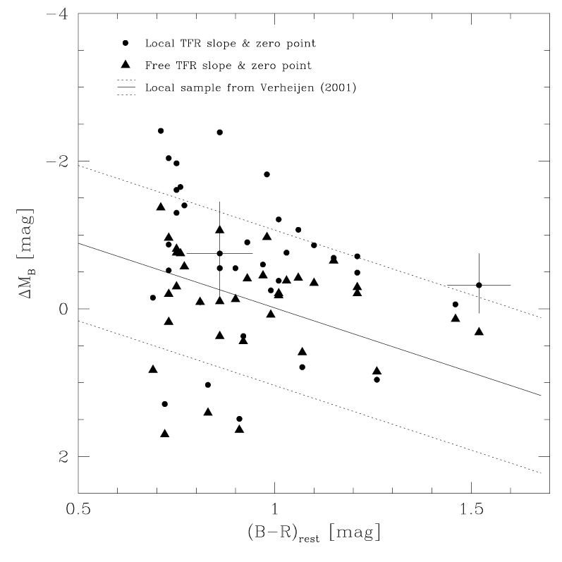
Figure 12: Offsets of the high quality FORS Deep Field sample from the local TFR by Verheijen (2001, circles), compared to the residuals of a free bisector fit to the high quality FDF data (triangles), both as a function of rest–frame color. The solid line represents the color–residual relation of the local Verheijen sample, the dotted lines denote the 3 $\sigma$ limits. Typical error bars are shown for two FDF objects.

The situation is changed if one assumes that the TFR slope and zero point could vary with cosmic time, i.e. if a free fit is applied to the distant sample. On the basis of the high quality data, a bootstrap bisector fit with 100 iterations yields

$$M_{B}=-(4.66\pm 0.67)\log V_{\rm max}-(10.43\pm 1.50).$$ (15)

To be consistent with the Verheijen sample, we performed the same fit using the intrinsic absorption convention by Tully et al. (Eq. 17) which yielded

$$M_{B}=-(5.22\pm 0.69)\log V_{\rm max}-(9.08\pm 1.56).$$ (16)

New residuals using this relation for the FDF sample were derived analogous to Eq. 10 and are compared to the initial values in Fig. 12. The residuals computed via Eq. 16 are mainly distributed within the range $-1\leq\Delta M_{B}\leq+1$ around zero, similar to the results given by Verheijen, though the scatter of the distant sample is larger and the correlation between color and residuals relatively weak. We conclude that the large offsets we find using Eq. 10, i.e. under the assumption of the local TFR slope and zero point, can hardly be attributed to the color–residual relation of local spirals.

Alternatively to an evolution of the TFR with look–back time, one possible interpretation could be that a fraction of the distant spirals are subject to galaxy–galaxy interactions, which could result in TF offsets of up to several magnitudes as stated by Kannappan et al. (Kan02b (2003)). To perform a search for galaxy pair candidates within our TF sample, we combined our complete data set (i.e. all galaxies with derived redshifts) with the lower resolution spectra from the FDF high–z campaign (Noll et al. No03 (2004)), yielding a total of 267 galaxies at $z<1$. As upper limits on the three–dimensional separation of two pair candidates, we adopted the results of Lambas et al. (La02 (2003)). Based on a data set of $\sim$ 10⁵ objects from the 2dF Galaxy Redshift Survey, the authors found that a projected distance $D_{\rm proj}\leq 100$ kpc and a relative radial velocity $\Delta V_{\rm sys}\leq 250$ km/s are reliable upper limits to select galaxy pairs with enhanced specific star formation.

12 spirals from the TF sample show spectroscopically confirmed neighbors within these limits. Of these galaxies, two are also possible members of the cluster at $z=0.33$ located in the southwestern corner of the FDF. We show the TF offsets of these pair/cluster candidates in comparison to the rest of the sample in Fig. 13. The two sub–samples seem to be similarly distributed. This is also implied by a two–dimensional Kolmogorov-Smirnov test which yields a propability of 0.31 that both subsamples are drawn from the same distribution function. We only observe a slight overrepresentation of pair/cluster candidates towards low rotation velocities. These are all spirals with RCs classified as low quality data, i.e. with relatively small radial extention and/or asymmetries. In total, only 5 out of 18 (corresponding to 28%) of the pair/cluster candidates have high quality curves, whereas for the rest of the sample this fraction accounts to 53%. This is in agreement with the results of Kannappan et al. (Kan02b (2003)), who find that a fraction of galaxies in close pairs show asymmetric or truncated RCs. We therefore reject the idea that a significant fraction of the galaxies with high quality RCs are subject to interactions.

The nearest neighbor search cannot yield all pairs at $z<1$ within the FDF, since we do not have spectroscopic redshifts on all galaxies in this regime (both the TF and the high–z study have a limit in apparent brightness). However, the aim of this test was to clarify whether the candidates which are identified differ from the rest of the sample. Since the five pair/cluster candidates included in the analysis show only moderate TF offsets, we conclude that it is unlikely that our high quality subsample introduces a bias towards overluminosities due to gravitational interactions.

Figure 13: Offsets of the FORS Deep Field spirals from the local TFR as given by Pierce & Tully (PT92 (1992)) as a function of maximum rotation velocity. The FDF sample is sub–divided according to environment: Squares denote potential members of a cluster at $z=0.33$, triangles are objects featuring neighboring galaxies within $\Delta V_{\rm sys}\leq 250$  km/s and $D_{\rm proj}\leq 100$ kpc and circles are probably isolated galaxies. Filled symbols denote objects with rotation curves that extend well into the region of constant rotation velocity at large radii.

8.2 Potential incompleteness effects

In the following, we will adress the question of whether the deficiency of our sample of objects with $M_{B}<-19$ and $\log V_{\rm max}>2.1$ (cf. Fig. 8) may be an observational bias.

For a magnitude–limited TF sample, not all objects within the field–of–view that are geometrically suitable enter the final data set. Towards the faint end of the observed luminosity distribution, the sample therefore is incomplete. At a fixed maximum rotation velocity, this may give rise to a bias against low–luminosity spirals and, in turn, lead to an underestimated TFR slope as pointed out by Giovanelli et al. (Gio97 (1997)).

Our apparent brightness limit of $R\leq 23^{m}$ corresponds to a limit in luminosity that is higher for larger redshifts. An impact of the incompleteness bias on our results should therefore coincide with a decrease of the TFR slope with increasing redshift. However, if we split the complete FDF sample into sets for objects with $z<0.45$ (41 galaxies) and $z>0.45$ (36 galaxies), the bootstrap fit slopes we find for the two are $a=-3.75\pm 0.44$ and $a=-3.77\pm 0.59$, respectively.

Potentially, our sample may introduce a bias against fast rotators of low luminosity. This is because the spatially resolved emission lines of large spirals (which on the average have higher $V_{\rm max}$ values) cover a larger CCD area and thus have lower signal–to–noise ratios per pixel than small spirals. For a given total line flux, the data set could therefore preferably contain slow rotators.

Since late–type spirals on average have stronger emission lines (and lower $V_{\rm max}$ values, see Sect. 8.5) than early–type spirals, this effect would induce a type–dependency of the TFR slope. For SED types $T\leq 3$, $T=5$ and $T\geq 8$, we find slopes of $a=-3.74\pm 1.40$, $a=-5.18\pm 0.63$ and $-4.78\pm 0.45$ (the large uncertainty of the first of these fits shows the influence of low number statistics). Although the 14 spirals of type Sb or earlier have a flatter tilt than the two other sub–sets, we do not find a significant correlation between spectrophotometric type and TFR slope within the derived errors of the bootstrap fits.

It is therefore unlikely that the shallower slope of the FDF sample with respect to the local data is an observational effect. We emphasize that, if the observed lack of distant spirals in the regime of low luminosities and fast rotation was due to such a bias, then the intrinsic scatter of the distant TF relation would have to be increased by a significant factor compared to the local universe, which we do not see.

8.3 Impact of the intrinsic RC shape

As stated in Sect. 4.4, the rotation velocities derived via the RC modelling are consistent for the “rise–turnover–flat” shape and the universal rotation curve from Persic & Salucci (PS91 (1991)), but slightly different if the URC as given in Persic et al. (PS96 (1996)) is used. However, if we restrict our sample to the high quality data, the difference between $V_{\rm max}$ and $V_{\rm opt}$ is negligible for spirals with $V_{\rm max}>150$ km/s, and amounts to only 5% in the median for the slow rotators. In effect, the TF offsets would be altered towards lower luminosities by only $\sim$ 0.15^m at $V_{\rm opt}=100$ km/s if the URC96 was used alternatively. None of our results would be affected significantly by such a small difference. For this reason, our analysis will be based on $V_{\rm max}$ throughout the section.

Another topic that has been referred to earlier are the slight differences between $\chi^{2}$-fits and “by–eye” fits of the synthetic to the observed rotation curves. Since the former yielded systematically lower maximum rotation velocities than the latter, the TF offsets would be brighter by $\sim\nobreak 0.25^{m}$ at $V_{\rm max}=100$ km/s if the analysis was based on the $V_{\rm max}$ values from $\chi^{2}$-fit RC modelling as introduced in Sect. 4.4. Therefore, if one assumes a “rise–turnover–flat” shape of the intrinsic RC, our approach of a by–eye comparsion between synthetic and observed RC yields conservative values of the TF offsets.

8.4 Influence of the intrinsic absorption correction

The convention we use for intrinsic absorption is purely inclination–dependent, as the optical depth and fractional dust disk thickness are held fixed for the entire sample. More recently, Tully et al. (Tu98 (1998)) and Karachentsev et al. (Ka02 (2002)) have found evidence for an internal extinction law which also depends on rotation velocity. These observations favour a higher amount of absorption in fast rotators than for spirals of low $V_{\rm max}$. If one assumes the relation $2V_{\rm max}\approx W^{i}_{R}$ between maximum rotation velocity and H I profile linewidth (see Tully & Fouqué TF85 (1985)), then equation 11 given in Tully et al. transforms into

$$A^{V,i}_{B}=2.75(\log V_{\rm max}-1.63)\log(a/b),$$ (17)

where $a$ and $b$ are the apparent major and minor axes, respectively. E.g., for a highly inclined disk with $i=80^{\circ}$, this yields 0.59^m at $V_{\rm max}=100$ km/s and 1.35^m at $V_{\rm max}=300$ km/s, whereas the initial Tully & Fouqué approach gives a value of $A^{i}_{B}=0.96^{m}$ independent of the maximum rotation velocity.

In effect, the slope of any TFR would be steeper if the intrinsic absorption is accounted for based on Eq. 17. But, since this mass–depedency is linear in $\log V_{\rm max}/M_{B}$–space, the slope change would affect distant and local sample consistently. This can be quantitatively verified with Eqs. 14 (the local Verheijen TFR) and 16 (the FDF high quality sample) which are both derived using the Tully et al. convention. Neither the median of the FDF spiral offsets from the local TFR (0.7 mag in the Tully et al. convention vs. 0.77 mag in the Tully & Fouqué convention) nor the evidence for a change in the distant TFR slope ($>$3$\sigma$ confidence level in both conventions) do significantly differ between the two approaches.

Since our results are therefore independent of the intrinsic absorption convention, we used the Tully & Fouqué approach throughout the paper for the sake of direct comparability with the previous studies.

8.5 A mass–dependent luminosity evolution?

It is well known that in the local universe, a dependency of $V_{\rm max}$ on galaxy type is observed. Blue, late–type spirals are on average slower rotators than red, early–type spirals (e.g. Rubin et al. Ru85 (1985)). For our sample, sub–divided according to SED type, we find respective median values of $\langle V_{\rm max}\rangle\approx 248$ km/s for $T\leq 3$, $\langle V_{\rm max}\rangle\approx 145$ km/s for $T=5$ and $\langle V_{\rm max}\rangle\approx 89$ km/s for $T\geq 8$. Since we observe a correlation between the TF offsets and $V_{\rm max}$, these $V_{\rm max}$ distributions imply a dependency of the mean luminosity offsets on SED type as is illustrated in Fig. 14.

Figure 14: Offsets of the FORS Deep Field sample from the local TFR as given by Pierce & Tully (PT92 (1992)) as a function of maximum rotation velocity, sub–divided according to SED type into Sb or earlier (squares), Sc (cicrles) and Sd or later (triangles), respectively. Filled symbols denote rotation curves which extend well out to the region of constant rotation velocity at large radii (labeled high quality data).

A consequence of this is a potential selection effect for small samples which mainly comprise a certain sub–type. If a data set was biased towards late–type spirals due to the target selection on blue colors (like, e.g., Simard & Pritchet SP98 (1998)) or strong emission lines (e.g. Rix et al. Rix97 (1997)), a considerable evolution in luminosity would be derived. On the other hand, if a data set preferably contains early–type spirals, i.e. large disks (Vogt et al. Vog96 (1996)), only a modest luminosity offset from the local TFR will be observed.

A straightforward interpretation of the correlation between the luminosity offsets and the maximum rotation velocity we find could be a change of the TFR slope with look–back time. As given in Sect. 8.1, a bootstrap bisector fit to the high quality FDF data yields a slope of $-4.66\pm 0.67$, corresponding to $>$99% confidence for a shallower slope at intermediate redshift with respect to the local PT92 sample. To verify this with a different fitting method, we estimate the errors of the absolute magnitudes to be

$$\sigma^{2}_{\rm TFR}=\sigma^{2}_{M_{B}}+7.48^{2}\sigma^{2}_{\log V_{\rm max}}.$$ (18)

The first term on the right hand side corresponds to Eq. 7 and the second term is the error propagation from the errors in $V_{\rm max}$ based on the PT92 slope. A linear $\chi^{2}$ -fit to the high quality FDF then gives

$$M_{B}=-(3.55\pm 0.41)\log V_{\rm max}-(12.84\pm 0.92),$$ (19)

i.e. the significance for a TFR slope change is even higher than on the basis of a bootstrap bisector fit.

As an explanation for the shallower slope at redshift $z\nobreak\approx\nobreak 0.5$, we will now discuss two alternatives. Firstly, our result may point to a luminosity evolution that depends on the maximum rotation velocity. According to simulations by van den Bosch (vdB03 (2002)), the total mass of a spiral galaxy within the virial radius can be estimated via

$$M_{\rm vir}=2.54\cdot 10^{10}M_{\odot}\Bigl{(}\frac{r_{\rm d}}{\rm kpc}\Bigr{)}\Bigl{(}\frac{V_{\rm max}}{100\,{\rm km/s}}\Bigr{)}^{2},$$ (20)

i.e. the correlation $\Delta M_{B}\propto\log V_{\rm max}$ implies $\Delta M_{B}\propto\log M_{\rm vir}$. For the spirals with high quality RCs, covering the range $3.2\nobreak\cdot\nobreak 10^{10}M_{\odot}\leq M_{\rm vir}\leq 1.6\cdot 10^{12}M_{\odot}$ ($\langle M_{\rm vir}\rangle=2.3\cdot 10^{11}M_{\odot}$), a linear $\chi^{2}$-fit yields

$$\Delta M_{B}=(1.14\pm 0.27)\log\frac{M_{\rm vir}}{M_{\odot}}-(13.46\pm 3.09).$$ (21)

Although the ground–based luminosity profile fits may place only upper limits on the scale lengths for some of the apparently smallest galaxies, we find evidence for a mass–dependent luminosity evolution which accounts to $\sim$ 2^m in rest–frame $B$  for the least massive objects and is negligible for high–mass spirals. This implies that the redshift dependency we observe (Eq. 11) is most probably a lower limit, since low-mass spirals — which show strong evolution in luminosity according to Eq. 21 — at higher redshifts will fall beyond our apparent brightness limit. For the same reason, we cannot speculate on a potential evolution (more precisely, a decrease) of the mean galaxy masses with redshift.

If one assumes that low–mass spirals have not undergone a significant increase of their metallicities since $z\nobreak\approx\nobreak 0.5$, our result is similar to that of Kobulnicky et al. (Ko03 (2003)), who used the distant luminosity–metallicity relation and found $\Delta M_{B}$ $\approx$ $-$1…$-$2 mag. On the other hand, Vogt (Vog01 (2001)) does not find a TFR slope change with a TF sample from the same survey (DEEP Groth Strip Survey).

Besides a mass–dependent luminosity evolution, a second possible explanation for the flatter tilt of the distant TFR could be a strongly starforming galaxy population within our sample that contributes less to the local luminosity density, i.e. either these galaxies could be overnumerous or overluminous at intermediate redshift. In terms of the luminosity function, this topic is well known as the “faint blue galaxy excess” (see Ellis Ell97 (1997) for an overview). Based on spectroscopic data from the Canada-France-Redshift-Survey, Driver et al. (Dri96 (1996)) found that dwarfs may have faded by over one magnitude between the regime $0.2<z<0.5$ and the local universe. These observational findings could be understood in terms of a reionization era between redshifts $z\approx 6$ and $z\approx 1$ which suppresses star formation in low–mass dark halos ($M_{\rm vir}\leq 10^{9}$ $M_{\odot}$, Babul & Rees BR92 (1992)).

However, only a small fraction of the high quality FDF sample could be members of such a blue dwarf population since the former covers the range $74\,{\rm km/s}\leavevmode\nobreak\ \leq\leavevmode\nobreak\ \log V_{\rm max}\leavevmode\nobreak\ \leq\leavevmode\nobreak\ 295\,{\rm km/s}$ and the lower virial mass limit of $3\cdot 10^{10}M_{\odot}$ also exceeds the dark halo mass range of dwarfs. Furthermore, the star formation rates derived from [OII] equivalent widths fall in the range $0.8\,M_{\odot}\,{\rm yr}^{-1}\leq{\rm SFR}\leq 18.3\,M_{\odot}\,{\rm yr}^{-1}$, with a median of $\sim$ 4.5 $M_{\odot}\,{\rm yr}^{-1}$, typical for massive local spirals (e.g. Kennicutt Ken83 (1983)).

If our result is interpreted in terms of a decreasing luminosity of low–mass spirals over the past $\sim$ 5 Gyrs (which accounts to the look–back time at $z\approx 0.5$), it could be due to a mass–dependent evolution of the mass–to–light ratio, or even a mass–age relation. A direct comparison to predictions of stellar population models is difficult since any evolution of the TFR introduces several competing effects. On the one hand, younger stellar populations coincide with a decrease of the mass–to–light ratio. On the other hand, since less gas has been consumed via star formation, the gas mass fraction most probably increases with look–back time, thereby increasing the mass–to–light ratio. Moreover, within the framework of hierarchical merging, disk sizes should be smaller for a given maximum rotation velocity and masses on the mean lower towards higher redshift (e.g. Mao et al. MMW98 (1998)). Based on the rotation velocity–size relation, i.e. the correlation between $V_{\rm max}$ and $r_{\rm d}$, our sample shows some evidence for slightly smaller disks at $z\approx 0.5$ (see Böhm et al. Boe03 (2003)). However, due to the limitations of the ground–based imaging, the significance of this evolution is low.

In effect, a decrease of the disk sizes and an increase of the gas mass fraction would tend to shift distant spirals to the low–luminosity side of the local TFR, whereas a lower stellar mass–to–light ratio would result in a shift to the high–luminosity side. A domination of the first two processes for fast rotators could explain why a fraction of the high–mass FDF spirals are underluminous in the TF diagram.

As already stated, the correlation between luminosity evolution and redshift given in Eq. 11 is probably only a conservative estimate. Because the disk sizes and gas fractions may also evolve, the pure luminosity evolution possibly is larger than approx. one magnitude between $z=1$ and the local universe. E.g., chemically consistent evolutionary synthesis models by Möller et al. (Moe01 (2001)) yield a luminosity evolution of $\sim$ 1.5 mag in rest–frame $B$ for an Sc spiral over this redshift range.

Although the mild evolution of the scale lengths that might be deduced from the FDF sample is in compliance with the “bottom–up” scheme of structure growth within the Cold Dark Matter hierarchical model, a luminosity evolution that is larger for low–mass galaxies would be in contradiction to it. If our result is interpreted in terms of younger ages (lower formation redshifts) for lower masses, the contradiction will be even more obvious. This is simply because small Dark Matter Halos should have formed earlier than large ones, and thus the stellar populations in galaxies of low mass should be older than those of high-mass systems. Semi–analytic simulations which account for a mass–dependent evolution of the stellar populations also yield an increase of TFR slope with look–back time (e.g. Ferreras & Silk FS01 (2001)).

On the other hand, it is well established and also valid for our sample that the colors of spirals tend to become redder with mass (beginning of this section) which is not reproduced by simulations within the hierarchical scenario unless the spectrophotometric properties of local spirals are used as a calibration (e.g. Bell et al. Be03 (2003)).

We therefore conclude that, if the TFR slope of our distant sample is related to a mass–dependant luminosity evolution, this would be at variance with the hierarchical merging scenario on small scales.

9 Conclusions

Using imaging data and spectroscopy taken with the ESO Very Large Telescope, we have derived structural parameters and resolved rotation curves of a magnitude–limited sample of 77 spiral galaxies in the FORS Deep Field. The objects cover the redshift range $0.1\leq z\leq 1.0$ and comprise all types from Sa to very late–type. Via a rotation curve modelling that takes into account geometric effects as well as seeing and optical beam smearing, the maximum rotation velocities have been derived and the distant $B$-band Tully–Fisher relation was constructed.

We find evidence for a luminosity evolution with look–back time which amounts to a brightening of $\Delta M_{B}\approx-1^{m}$ at redshift unity. Moreover, we observe a correlation between the luminosity evolution and the total masses. The distant low–mass spirals are brighter by up to two magnitudes than their local counterparts, whereas the luminosity evolution of high–mass systems is negligible. In effect, the slope of the Tully–Fisher relation at intermediate redshift is shallower than for local samples. This may partly be caused by a population of small, starforming galaxies that contribute less to the luminosity density in the local universe. Nevertheless, the vast majority of our objects have virial masses too large to be dwarf galaxies and show star formation rates typical of normal spirals. The flatter tilt we find for the distant Tully–Fisher relation is in contradiction to the predictions of recent semi–analytic simulations.

- (1) Babul, A., & Rees, M. J. 1992, MNRAS, 255, 346
- (2) Barden, M., Lehnert, M. D., Tacconi, L., et al. 2003, ApJL, submitted (astro-ph/0302392)
- (3) Bender, R., Appenzeller, I., Böhm, A., et al. 2001, The FORS Deep Field: Photometric redshifts and object classification, in Deep Fields, ed. S. Cristiani, A. Renzini, & R. E. Williams, ESO astrophysics symposia (Springer), 96
- (4) Bell, E. F., Baugh, C. M., Cole, S., et al. 2003, MNRAS, 343, 367
- (5) Bertin, E., & Arnouts, S. 1996, A&AS, 117, 393
- (6) Boissier, S., & Prantzos, N. 2001, MNRAS, 325, 321
- (7) Böhm, A., Ziegler, B. L., Fricke, K. J., et al. 2003, Ap&SS, 284, 689
- (8) Burstein, D., Bender, R., Faber, S. M., & Nolthenius, R. 1997, AJ, 114, 1365
- (9) Cardelli, J. A., Clayton, G. C., Mathis J. S. 1989, ApJ, 345, 245
- (10) Contardo, G., Steinmetz, M., & Fritze-v.Alvensleben, U. 1998, ApJ, 507, 497
- (11) Courteau, S. 1997, AJ, 114, 2402
- (12) Dopita, M. A., & Ryder, S. D. 1994, ApJ, 430, 163
- (13) Dressler, A., Lynden-Bell, D., Burstein, D., et al. 1987, ApJ, 313, 42
- (14) Driver, S. P., et al. 1996, ApJ, 466, L5
- (15) Ellis, R. S. 1997, ARA&A, 35, 389
- (16) Ferreras, I., & Silk, J. 2001, ApJ, 557, 165
- (17) Frei, Z., & Gunn, J. E. 1994, AJ, 108, 1476
- (18) Fukugita, M., Shimasaku, K., & Ichikawa, T. 1995, PASP, 107, 945
- (19) Giovanelli, R., Haynes, M. P., Herter, T., et al. 1997, AJ, 113, 53
- (20) Haynes, M. P., Giovanelli, R., Chamaraux, P., et al. 1999, AJ, 117, 2039
- (21) Heidt, J., Appenzeller, I., Gabasch, A., et al. 2003, A&A, 398, 49
- (22) Jimenez, R., Padoan, P., Matteucci, F., Heavens, A. 1998, MNRAS, 299, 123
- (23) Kannappan, S. J., Fabricant, D. G., & Franx, M. 2002, AJ, 123, 2358
- (24) Kannappan, S. J., Barton Gillespie, E., Fabricant, D. G., Franx, M., & Vogt, N. P. 2003, Interpreting Offsets from the Tully–Fisher Relation, in Galaxy Evolution: Theory and Observations, ed. V. Avila-Resse, C. Firmani, C. S. Frenk, & C. Allen, RevMexAA, 17, 188
- (25) Karachentsev, I. D., Mitronova, S. N., Karachentseva, V. E., Kudrya, Y. N., & Jarrett, T. H. 2002, A&A, 396, 431
- (26) Kennicutt, R. C. 1992a, ApJS, 79, 255
- (27) Kennicutt, R. C. 1992b, ApJ, 388, 310
- (28) Kennicutt, R. C. 1983, ApJ, 272, 54
- (29) Kobulnicky, H. A., Willmer, C. N. A., Phillips, A. C., et al. 2003, ApJ, 599, 1006
- (30) Koda, J., Sofue, Y., & Wada, K. 2000, ApJ, 531, L17
- (31) Kodeira, K., & Watanabe, M. 1988, AJ, 96, 1593
- (32) Koo, D. C. 2001, DEEP: Pre–DEIMOS Surveys to I 24 of Galaxy Evolution and Kinematics, in Deep Fields, ed. S. Cristiani, A. Renzini, & R. E. Williams, ESO astrophysics symposia (Springer), 107
- (33) Kron, R. G. 1980, ApJS, 43, 305
- (34) Lambas, D. G., Tissera, P. B., Sol Alonso, M., & Coldwell, G. 2003, MNRAS, 346, 1189
- (35) Mao, S., Mo, H. J., & White, S. D. M. 1998, MNRAS, 297, L71
- (36) Marleau, F. R., & Simard, L. 1998, ApJ, 507, 585
- (37) Mathewson, D. S., & Ford, V. L. 1996, ApJS, 107, 97
- (38) Mehlert, D., Noll, S., Appenzeller, I., et al. 2002, A&A, 393, 809
- (39) Milvang-Jensen, B., 2003, PhD thesis, University of Nottingham
- (40) Milvang-Jensen, B., Aragón-Salamanca, A., Hau, G. K. T., Jørgensen, I., & Hjorth, J. 2003, MNRAS, 339, L1
- (41) Möller, C. S., Fritze-v.Alvensleben, U., Fricke, K. J., & Calzetti, D. 2001, Ap&SS, 276, 799
- (42) Navarro, J. F., & Steinmetz, M. 2000, ApJ 538, 477
- (43) Noll, S., Mehlert, D., Appenzeller, I., et al. 2004, A&A, accepted (astro-ph/0401500)
- (44) Peebles, P. J. E. 1993, Principles of Physical Cosmology (Princeton University Press)
- (45) Persic, M., & Salucci, P. 1991, ApJ, 368, 60 (URC91)
- (46) Persic, M., & Salucci, P., & Stel, F. 1996, MNARS, 281, 27 (URC96)
- (47) Pierce, M. J., & Tully, R. B. 1992, ApJ, 387, 47 (PT92)
- (48) Rix, H.-W., Guhathakurta, P., Colless, M., & Ing, K. 1997, MNRAS, 285, 779
- (49) Rubin, V. C., Burstein, D., Ford Jr., W. K., & Thonnard, N. 1985, ApJ, 289, 81
- (50) Ryder, S. D., & Dopita, M. A. 1994, ApJ, 430, 142
- (51) Sakai, S., et al. 2000, ApJ, 529, 698
- (52) Simard, L., & Pritchet, C. J. 1998, ApJ, 505, 96
- (53) Simard, L., & Pritchet, C. J. 1999, PASP, 111, 453
- (54) Simard, L., Willmer, C. N., Vogt, N. P., et al. 2002, ApJS, 142, 1
- (55) Tully, R. B., & Fisher, J. R. 1977, A&A, 54, 661
- (56) Tully, R. B., & Fouqué, P. 1985, ApJS, 58, 67
- (57) Tully, R. B., Pierce, M. J., Huang, J.-S., et al. 1998, AJ, 115, 2264
- (58) van den Bosch, F. C. 2002, MNRAS, 332, 456
- (59) Verheijen, M. A. W. 2001, ApJ, 563, 694
- (60) Vogt, N. P. 2001, Distant Disk Galaxies: Kinematics and Evolution to z1, in Deep Fields, ed. S. Cristiani, A. Renzini, & R. E. Williams, ESO astrophysics symposia (Springer), 112
- (61) Vogt, N. P., Forbes, D. A., Phillips, A. C., et al. 1996, ApJ, 465, L15
- (62) Vogt, N. P., Phillips, A. C., Faber, S. M., et al. 1997, ApJ, 479, L121
- (63) Williams, R. E., Blacker, B., Dickinson, M., et al. 1996, AJ, 112, 1335
- (64) Ziegler, B. L., Böhm, A., Fricke, K. J., et al. 2002, ApJ, 564, L69