Large-scale surveys and
cosmic structure

Abstract

These lectures deal with our current knowledge of the matter distribution in the universe, focusing on how this is studied via the large-scale structure seen in galaxy surveys. We first assemble the necessary basics needed to understand the development of density fluctuations in an expanding universe, and discuss how galaxies are located within the dark-matter density field. Results from the 2dF Galaxy Redshift Survey are presented and contrasted with theoretical models. We show that the combination of large-scale structure and data on microwave-background anisotropies can eliminate almost all degeneracies, and yield a completely specified cosmological model. This is the ‘concordance’ universe: a geometrically flat combination of vacuum energy and cold dark matter. The study of cosmic structure is able to establish this in a manner independent of external information, such as the Hubble diagram; this extra information can however be used to limit non-standard alternatives, such as a variable equation of state for the vacuum.

1 Preamble

1.1 The perturbed universe

It has been clear since the 1930s that galaxies are not distributed at random in the universe (Hubble 1934). For decades, our understanding of this fact was limited by the lack of a three-dimensional picture, although some impressive progress was made: the dedication of pioneers such as Shane & Wirtanen in compiling galaxy catalogues by eye is humbling to consider. However, studies of the galaxy distribution came of age in the 1980s, via redshift surveys, in which Hubble’s $v=Hd$ law is used to turn spectroscopic redshifts into estimates of distance (e.g. Davis & Peebles 1983; de Lapparant, Geller & Huchra 1986; Saunders et al. 1991). We were then able to see clearly (e.g. figure 1) a wealth of large-scale structures of size exceeding 100 Mpc. The existence of these cosmological structures must be telling us something important about the initial conditions of the big bang, and about the physical processes that have operated subsequently. These lectures cover some of what we have learned in this regard.

Figure 1: One of the iconic pictures of the large-scale structure in the galaxy distribution is this slice made from John Huchra’s ZCAT compilation of galaxy redshifts, reflecting the state of our knowledge in the mid-1980s. The survey coverage is not quite complete; as well as the holes due to the galactic plane around right ascensions $6^{\rm h}$ and $19^{\rm h}$, the rich clusters are somewhat over-represented with respect to a true random sampling of the galaxy population. Nevertheless, this plot emphasizes nicely both the large-scale features such as the ‘great wall’ on the left, the totally empty void regions, and the radial ‘fingers of God’ caused by virialized motions in the clusters. One of the principal challenges in cosmology is to explain this pattern.

Throughout, it will be convenient to adopt a notation in which the density (of mass, light, or any property) is expressed in terms of a dimensionless density perturbation $\delta$:

$${1+\delta({\bf x})\equiv\rho({\bf x})/\langle\rho\rangle,}$$ (1)

where $\langle\rho\rangle$ is the global mean density. The quantity $\delta$ need not be small, but writing things in this form naturally suggests an approach via perturbation theory in the important linear case where $\delta\ll 1$. As we will see, this was a good approximation at early times. The existence of this field in the universe raises two questions: what generated it, and how does it evolve? A popular answer for the first question is inflation, in which quantum fluctuations are able to seed density fluctuations. So far, despite some claims, this theory is not tested, and we consider later some ways in which this might be accomplished. Mainly, however, we will be concerned here with the question of evolution.

1.2 Relativistic viewpoint and gauge issues

Many of the key aspects of the evolution of structure in the universe can be dealt with via a deceptively simple Newtonian approach, but honesty requires a brief overview of some of the difficult issues that will be evaded by taking this route.

Because relativistic physics equations are written in a covariant form in which all quantities are independent of coordinates, relativity does not distinguish between active changes of coordinate (e.g. a Lorentz boost) or passive changes (a mathematical change of variable, normally termed a gauge transformation). This generality is a problem, since it is not trivial to know which coordinates should be used. To see how the problems arise, ask how tensors of different order change under a gauge transformation $x^{\mu}\rightarrow x^{\prime}{}^{\mu}=x^{\mu}+\epsilon^{\mu}$. Consider first a scalar quantity $S$ (which might be density, temperature etc.). A scalar quantity in relativity is normally taken to be independent of coordinate frame, but this is only for the case of Lorentz transformations, which do not involve a change of the spacetime origin. A gauge transformation therefore not only induces the usual transformation coefficients $dx^{\prime}{}^{\mu}/dx^{\nu}$, but also involves a translation that relabels spacetime points. We therefore have to deal with $S^{\prime}(x^{\mu}+\epsilon^{\mu})=S(x^{\mu})$, so the rule for the gauge transformation of scalars is

$$S^{\prime}(x^{\mu})=S(x^{\mu})-\epsilon^{\alpha}\partial S/\partial x^{\alpha}.$$ (2)

Similar reasoning yields the gauge transformation laws for higher tensors, although we need to account not only for the translation of the origin, but also for the usual effect of the coordinate transformation on the tensor.

Consider applying this to the case of a uniform universe; here $\rho$ only depends on time, so that

$$\rho^{\prime}=\rho-\epsilon^{0}\dot{\rho}.$$ (3)

An effective density perturbation is thus produced by a local alteration in the time coordinate: when we look at a universe with a fluctuating density, should we really think of a uniform model in which time is wrinkled? This ambiguity may seem absurd, and in the laboratory it could be resolved empirically by constructing the coordinate system directly – in principle by using light signals. This shows that the cosmological horizon plays an important role in this topic: perturbations with wavelength $\lambda\mathrel{\lower 2.58334pt\hbox{$\buildrel{\textstyle<}\over{\scriptstyle\sim}$}}ct$ inhabit a regime in which gauge ambiguities can be resolved directly via common sense. The real difficulties lie in the super-horizon modes with $\lambda\mathrel{\lower 2.58334pt\hbox{$\buildrel{\textstyle>}\over{\scriptstyle\sim}$}}ct$. However, at least within inflationary models, these difficulties can be overcome. According to inflation, perturbations on scales greater than the horizon were originally generated via quantum fluctuations on small scales within the horizon of a nearly de Sitter exponential expansion. There is thus no problem in understanding how the initial density field is described, since the simplest coordinate system can once again be constructed directly.

The most direct way of solving these difficulties is to construct perturbation variables that are explicitly independent of gauge. Comprehensive technical discussions of this method are given by Bardeen (1980), Kodama & Sasaki (1984), Mukhanov, Feldman & Brandenberger (1992). The starting point for a discussion of metric perturbations is to devise a notation that will classify the possible perturbations. Since the metric is symmetric, there are 10 independent degrees of freedom in $g^{\mu\nu}$; a convenient scheme that captures these possibilities is to write the cosmological metric as

$$d\tau^{2}=a^{2}(\eta)\left\{(1+2\phi)d\eta^{2}+2w_{i}d\eta\,dx^{i}-\left[(1-2\psi)\gamma_{ij}+2h_{ij}\right]dx^{i}\,dx^{j}\right\}.$$ (4)

In this equation, $\eta$ is conformal time, and $\gamma_{ij}$ is the comoving spatial part of the Robertson-Walker metric.

The total number of degrees of freedom here is apparently 2 (scalar fields $\phi$ and $\psi$) + 3 (3-vector field $\bf w$) + 6 (symmetric 3-tensor $h_{ij}$) $=11$. To get the right number, the tensor $h_{ij}$ is required to be traceless: $\gamma^{ij}h_{ij}=0$. The perturbations can be split into three classes: scalar perturbations, which are described by scalar functions of spacetime coordinate, and which correspond to the growing density perturbations studied above; vector perturbations, which correspond to vorticity perturbations, and tensor perturbations, which correspond to gravitational waves. Here, we shall concentrate mainly on scalar perturbations. Since vectors and tensors can be generated from derivatives of a scalar function, the most general scalar perturbation actually makes contributions to all the $g_{\mu\nu}$ components in the above expansion:

$$\delta g_{\mu\nu}=a^{2}\,\left(\matrix{2\phi&-B_{,i}\cr-B_{,i}&2[\psi\delta_{ij}-E_{,ij}]\cr}\right),$$ (5)

where four scalar functions $\phi$, $\psi$, $E$ and $B$ are involved. It turns out that this situation can be simplified by defining variables that are unchanged by a gauge transformation:

  $${\Phi} {{}\equiv\phi+{1\over a}\;[(B-E^{\prime})a]^{\prime}} {\Psi} {{}\equiv\psi-{a^{\prime}\over a}\ (B-E^{\prime}),}$$   (6)

where primes denote derivatives with respect to conformal time.

These gauge-invariant ‘potentials’ have a fairly direct physical interpretation, since they are closely related to the Newtonian potential. The easiest way to evaluate the gauge-invariant fields is to make a specific gauge choice and work with the longitudinal gauge in which $E$ and $B$ vanish, so that $\Phi=\phi$ and $\Psi=\psi$. A second key result is that inserting the longitudinal metric into the Einstein equations shows that $\phi$ and $\psi$ are identical in the case of fluid-like perturbations where off-diagonal elements of the energy–momentum tensor vanish. In this case, the longitudinal gauge becomes identical to the Newtonian gauge, in which perturbations are described by a single scalar field, which is the gravitational potential. The conclusion is thus that the gravitational potential can for many purposes give an effectively gauge-invariant measure of cosmological perturbations, and this provides a sounder justification for the Newtonian approach that we now adopt.

2 Newtonian equations of motion

2.1 Matter-dominated universe

In the Newtonian approach, we treat dynamics of cosmological matter exactly as we would in the laboratory, by finding the equations of motion induced by either pressure or gravity. In what follows, it should be remembered that we probably need to deal in practice with two rather different kinds of material: dark matter that is collisionless and interacts only via gravity, and baryonic material which is a collisional fluid, coupled to dark matter only via gravity (and to photons via Thomson scattering, so that the dominant part of the pressure derives from the radiation).

Also, the problem of cosmological dynamics has to deal with the characteristic feature of the Hubble expansion. This means that it is convenient to introduce comoving length units, and to consider primarily peculiar velocities – i.e. deviations from the Hubble flow. The standard notation that includes these aspects is

  $${{\bf x}(t)} {{}=a(t){\bf r}(t)} {{\bf\delta v}(t)} {{}=a(t){\bf u}(t),}$$   (7)

so that ${\bf x}$ has units of proper length, i.e. it is an Eulerian coordinate. First note that the comoving peculiar velocity $\bf u$ is just the time derivative of the comoving coordinate $\bf r$:

$$\dot{\bf x}=\dot{a}{\bf r}+a\dot{\bf r}=H{\bf x}+a\dot{\bf r},$$ (8)

where the rhs must be equal to the Hubble flow $H{\bf x}$, plus the peculiar velocity $\delta{\bf v}=a{\bf u}$. In this equation, dots stand for exact convective time derivatives – i.e. time derivatives measured by an observer who follows a particle’s trajectory – rather than partial time derivatives $\partial/\partial t$.

The equation of motion follows from writing the Eulerian equation of motion as $\ddot{\bf x}={\bf g_{\rm 0}+g}$, where ${\bf g}=-\nabla\Phi/a$ is the peculiar acceleration, and $\bf g_{\rm 0}$ is the acceleration that acts on a particle in a homogeneous universe (neglecting pressure forces to start with, for simplicity). Differentiating ${\bf x}=a{\bf r}$ twice gives

$$\ddot{\bf x}=a\dot{\bf u}+2\dot{a}{\bf u}+{\ddot{a}\over a}\,{\bf x}={\bf g_{\rm 0}+g}.$$ (9)

The unperturbed equation corresponds to zero peculiar velocity and zero peculiar acceleration: $(\ddot{a}/a)\,{\bf x}={\bf g_{\rm 0}}$; subtracting this gives the perturbed equation of motion

$$\dot{\bf u}+2(\dot{a}/a){\bf u}={\bf g}/a.$$ (10)

The only point that needs a little more thought is the nature of the unperturbed equation of motion. This cannot be derived from Newtonian gravity alone, since general relativity is really needed for a proper derivation of the homogeneous equation of motion. However, as long as we are happy to accept that $\bf g_{\rm 0}$ is given, then it is a well-defined procedure to add a peculiar acceleration that is the gradient of the potential derived from the density perturbations.

The equation of motion for the peculiar velocity shows that $\bf u$ is affected by gravitational acceleration and by the Hubble drag term, $2(\dot{a}/a){\bf u}$. This arises because the peculiar velocity falls with time as a particle attempts to catch up with successively more distant (and therefore more rapidly receding) neighbours. If the proper peculiar velocity is $v$, then after time $dt$ the galaxy will have moved a proper distance $x=v\,dt$ from its original location. Its near neighbours will now be galaxies with recessional velocities $H\,x=H\,v\,dt$, relative to which the peculiar velocity will have fallen to $v-Hx$. The equation of motion is therefore just

$$\dot{v}=-H\,v=-{\dot{a}\over a}\,v,$$ (11)

with the solution $v\propto a^{-1}$: peculiar velocities of nonrelativistic objects suffer redshifting by exactly the same factor as photon momenta. This becomes $\dot{u}=-2H\,u$ when rewritten in comoving units.

The peculiar velocity is directly related to the evolution of the density field, through conservation of mass. This is expressed via the continuity equation, which takes the form

$${d\over dt}\rho_{0}(1+\delta)=-\rho_{0}(1+\delta)\,{\bf\nabla\cdot u}.$$ (12)

Here, spatial derivatives are with respect to comoving coordinates:

$$\nabla\equiv a\,\nabla_{\rm proper},$$ (13)

which we will assume hereafter, and the time derivative is once more a convective one:

$${d\over dt}={\partial\over\partial t}+{\bf u\cdot\nabla}.$$ (14)

Finally, when using comoving length units, the background density $\rho_{0}$ independent of time, and so the full continuity equation can be written as

$${d\over dt}\delta=-(1+\delta){\bf\nabla\cdot u}.$$ (15)

Unlike the equation of motion for $\bf u$, this is not linear in the perturbations $\delta$ and $\bf u$. To cure this, we restrict ourselves to the case $\delta\ll 1$ and linearize the equation, neglecting second-order terms like $\delta\times{\bf u}$, which removes the distinction between convective and partial time derivatives. The linearized equations for conservation of momentum and matter as experienced by fundamental observers moving with the Hubble flow are then:

  $${{}\dot{\bf u}+2{\dot{a}\over a}\,{\bf u}={{\bf g}\over a}} {{}\dot{\delta}=-{\bf\nabla\cdot u},}$$   (16)

where the peculiar gravitational acceleration $-{\bf\nabla}\Phi/a$ is denoted by $\bf g$.

The solutions of these equations can be decomposed into modes either parallel to $\bf g$ or independent of $\bf g$ (these are the homogeneous and inhomogeneous solutions to the equation of motion). The homogeneous case corresponds to no peculiar gravity – i.e. zero density perturbation. This is consistent with the linearized continuity equation, ${\bf\nabla\cdot u}=-\dot{\delta}$, which says that it is possible to have vorticity modes with ${\bf\nabla\cdot u}=0$ for which $\dot{\delta}$ vanishes, so there is no growth of structure in this case. The proper velocities of these vorticity modes decay as $v=au\propto a^{-1}$, as with the kinematic analysis for a single particle.

Growing mode  For the growing mode, it is most convenient to eliminate $\bf u$ by taking the divergence of the equation of motion for $\bf u$, and the time derivative of the continuity equation. This requires a knowledge of $\bf\nabla\cdot g$, which comes via Poisson’s equation: ${\bf\nabla\cdot g}=4\pi Ga\rho_{0}\delta$. The resulting 2nd-order equation for $\delta$ is

$$\ddot{\delta}+2{\dot{a}\over a}\dot{\delta}=4\pi G\rho_{0}\,\delta.$$ (17)

This is easily solved for the $\Omega_{m}=1$ case, where $4\pi G\rho_{0}=3H^{2}/2=2/3t^{2}$, and a power-law solution works:

$$\delta(t)\propto t^{2/3}\quad{\rm or}\quad t^{-1}.$$ (18)

The first solution, with $\delta(t)\propto a(t)$ is the growing mode, corresponding to the gravitational instability of density perturbations. Given some small initial seed fluctuations, this is the simplest way of creating a universe with any desired degree of inhomogeneity.

An alternative way of looking at the growing mode is that we want to try looking for a homogeneous solution ${\bf u}=F(t)\bf g$. Then using continuity plus ${\bf\nabla\cdot g}=4\pi Ga\rho_{0}\delta$, gives us

$${\bf\delta v}={2f(\Omega_{m})\over 3H\Omega_{m}}{\bf g},$$ (19)

where the function $f(\Omega_{m})\equiv d\ln\delta/d\ln a$. A very good approximation to this (Peebles 1980) is $f\simeq\Omega^{0.6}$ (a result that is almost independent of $\Lambda$; Lahav et al. 1991).

Jeans scale  So far, we have mainly considered the collisionless component. For the photon-baryon gas, all that changes is that the peculiar acceleration gains a term from the pressure gradients:

$${\bf g}=-{\bf\nabla}\Phi/a-{\bf\nabla}p/(a\rho_{0}).$$ (20)

The pressure fluctuations are related to the density perturbations via the sound speed

$$c_{s}^{2}\equiv{\partial p\over\partial\rho}.$$ (21)

Now think of a plane-wave disturbance $\delta\propto e^{-i{\bf k\cdot r}}$, where $\bf k$ is a comoving wavevector; in other words, suppose that the wavelength of a single Fourier mode stretches with the universe. All time dependence is carried by the amplitude of the wave, and so the spatial dependence can be factored out of time derivatives in the above equations (which would not be true with a constant comoving wavenumber $k/a$). The equation of motion for $\delta$ then gains an extra term on the rhs from the pressure gradient:

$${\ddot{\delta}+2{\dot{a}\over a}\dot{\delta}=\delta\bigl{(}4\pi G\rho_{0}-c_{s}^{2}k^{2}/a^{2}\bigr{)}.}$$ (22)

This shows that there is a critical proper wavelength, the Jeans length, at which we switch from the possibility of gravity-driven growth for long-wavelength modes to standing sound waves at short wavelengths. This critical length is

$${\lambda_{\rm\scriptscriptstyle J}={2\pi\over k_{\rm\scriptscriptstyle J}a}=c_{s}\sqrt{{\pi\over G\rho}}.}$$ (23)

Qualitatively, we expect to have no growth when the ‘driving term’ on the rhs is negative. However, owing to the expansion, $\lambda_{\rm\scriptscriptstyle J}$ will change with time, and so a given perturbation may switch between periods of growth and stasis. These effects help to govern the form of the perturbation spectrum that propagates to the present universe from early times.

The general case  How does the matter-dominated growth $\delta(a)\propto a$ change at late times when $\Omega_{m}\neq 1$? The differential equation for $\delta$ is as before, but $a(t)$ is altered. Provided the vacuum equation of state is exactly $p=-\rho c^{2}$, or if the vacuum energy is negligible, the solutions to the growth equations can be written as

$${\delta\propto\cases{({\dot{a}/a})\,\int_{0}^{a}(\dot{a})^{-3}\,da\quad\;&(growing mode)\cr({\dot{a}/a})\quad\;&(decaying mode).\cr}}$$ (24)

(Heath 1977; see also section 10 of Peebles 1980). For the most general case, e.g. a vacuum with time-varying density, these do not apply, and the differential equation for $\delta$ must be integrated directly.

In any case, the equation for the growing mode requires numerical integration unless the vacuum energy vanishes. A very good approximation to the answer is given by Carroll et al. (1992):

$${{\delta(z=0,\Omega)\over\delta(z=0,\Omega=1)}\simeq\frac{5}{2}\Omega_{m}\left[\Omega_{m}^{4/7}-\Omega_{v}+(1+\frac{1}{2}\Omega_{m})(1+\frac{1}{70}\Omega_{v})\right]^{-1}.}$$ (25)

This fitting formula for the growth suppression in low-density universes is an invaluable practical tool. For flat models with $\Omega_{m}+\Omega_{v}=1$, it says that the growth suppression is less marked than for an open universe – approximately $\Omega^{0.23}$ as against $\Omega^{0.65}$ in the $\Lambda=0$ case. This reflects the more rapid variation of $\Omega_{v}$ with redshift; if the cosmological constant is important dynamically, this only became so very recently, and the universe spent more of its history in a nearly Einstein–de Sitter state by comparison with an open universe of the same $\Omega_{m}$.

2.2 Radiation-dominated universe

At early enough times, the universe was radiation dominated ($c_{s}=c/\sqrt{3}$) and the analysis so far does not apply. It is common to resort to general relativity perturbation theory at this point. However, the fields are still weak, and so it is possible to generate the results we need by using special relativity fluid mechanics and Newtonian gravity with a relativistic source term:

$$\nabla^{2}\Phi=4\pi G(\rho+3p/c^{2}),$$ (26)

in Eulerian units. The main change from the previous treatment come from factors of 2 and $4/3$ due to this $(\rho+3p/c^{2})$ term, and other contributions of the pressure to the relativistic equation of motion. The resulting evolution equation for $\delta$ is

$${\ddot{\delta}+2{\dot{a}\over a}\dot{\delta}={32\pi\over 3}G\rho_{0}\delta,}$$ (27)

so the net result of all the relativistic corrections is a driving term on the rhs that is a factor $8/3$ higher than in the matter-dominated case (see e.g. Section 15.2 of Peacock 1999 for the details).

In both matter- and radiation-dominated universes with $\Omega=1$, we have $\rho_{0}\propto 1/t^{2}$:

  $${{\rm matter\ domination}\ (a\propto t^{2/3}):\quad} {{}4\pi G\rho_{0}={2\over 3t^{2}}} {{\rm radiation\ domination}\ (a\propto t^{1/2}):\quad} {{}32\pi G\rho_{0}/3={1\over t^{2}}.}$$   (28)

Every term in the equation for $\delta$ is thus the product of derivatives of $\delta$ and powers of $t$, and a power-law solution is obviously possible. If we try $\delta\propto t^{n}$, then the result is $n=2/3$ or $-1$ for matter domination; for radiation domination, this becomes $n=\pm 1$. For the growing mode, these can be combined rather conveniently using the conformal time $\eta\equiv\int dt/a$:

$${\delta\propto\eta^{2}.}$$ (29)

The quantity $\eta$ is proportional to the comoving size of the cosmological particle horizon.

One further way of stating this result is that gravitational potential perturbations are independent of time (at least while $\Omega=1$). Poisson’s equation tells us that $-k^{2}\Phi/a^{2}\propto\rho\,\delta$; since $\rho\propto a^{-3}$ for matter domination or $a^{-4}$ for radiation, that gives $\Phi\propto\delta/a$ or $\delta/a^{2}$ respectively, so that $\Phi$ is independent of $a$ in either case. In other words, the metric fluctuations resulting from potential perturbations are frozen, at least for perturbations with wavelengths greater than the horizon size.

2.3 Mészáros effect

What about the case of collisionless matter in a radiation background? The fluid treatment is not appropriate here, since the two species of particles can interpenetrate. A particularly interesting limit is for perturbations well inside the horizon: the radiation can then be treated as a smooth, unclustered background that affects only the overall expansion rate. This is analogous to the effect of $\Lambda$, but an analytical solution does exist in this case. The perturbation equation is as before

$$\ddot{\delta}+2{\dot{a}\over a}\dot{\delta}=4\pi G\rho_{m}\delta,$$ (30)

but now $H^{2}=8\pi G(\rho_{m}+\rho_{r})/3$. If we change variable to $y\equiv\rho_{m}/\rho_{r}=a/a_{\rm eq}$, and use the Friedmann equation, then the growth equation becomes

$$\delta^{\prime\prime}+{2+3y\over 2y(1+y)}\,\delta^{\prime}-{3\over 2y(1+y)}\,\delta=0$$ (31)

(for $k=0$, as appropriate for early times). It may be seen by inspection that a growing solution exists with $\delta^{\prime\prime}=0$:

$${\delta\propto y+2/3.}$$ (32)

It is also possible to derive the decaying mode. This is simple in the radiation-dominated case ($y\ll 1$): $\delta\propto-\ln y$ is easily seen to be an approximate solution in this limit.

What this says is that, at early times, the dominant energy of radiation drives the universe to expand so fast that the matter has no time to respond, and $\delta$ is frozen at a constant value. At late times, the radiation becomes negligible, and the growth increases smoothly to the Einstein–de Sitter $\delta\propto a$ behaviour (Mészáros 1974). The overall behaviour is therefore similar to the effects of pressure on a coupled fluid: for scales greater than the horizon, perturbations in matter and radiation can grow together, but this growth ceases once the perturbations enter the horizon. However, the explanations of these two phenomena are completely different. In the fluid case, the radiation pressure prevents the perturbations from collapsing further; in the collisionless case, the photons have free-streamed away, and the matter perturbation fails to collapse only because radiation domination ensures that the universe expands too quickly for the matter to have time to self-gravitate. Because matter perturbations enter the horizon (at $y=y_{\rm entry}$) with $\dot{\delta}>0$, $\delta$ is not frozen quite at the horizon-entry value, and continues to grow until this initial ‘velocity’ is redshifted away, giving a total boost factor of roughly $\ln y_{\rm entry}$. This log factor may be seen below in the fitting formulae for the CDM power spectrum.

2.4 Coupled perturbations

We will often be concerned with the evolution of perturbations in a universe that contains several distinct components (radiation, baryons, dark matter). It is easy to treat such a mixture if only gravity is important (i.e. for large wavelengths). Look at the perturbation equation in the form

$$L\,\delta={\rm driving\ term},\quad\quad L\equiv{\partial^{2}\over\partial t^{2}}+{2\dot{a}\over a}{\partial\over\partial t}.$$ (33)

The rhs represents the effects of gravity, and particles will respond to gravity whatever its source. The coupled equations for several species are thus given by summing the driving terms for all species.

Matter plus radiation  The only subtlety is that we must take into account the peculiarity that radiation and pressureless matter respond to gravity in different ways, as seen in the equations of fluid mechanics. The coupled equations for perturbation growth are thus

$$L\left({\delta_{m}\atop\delta_{r}}\right)=4\pi G\left(\matrix{\rho_{m}&2\rho_{r}\cr 4\rho_{m}/3&8\rho_{r}/3\cr}\right)\left({\delta_{m}\atop\delta_{r}}\right).$$ (34)

Solutions to this will be simple if the matrix has time-independent eigenvectors. Only one of these is in fact time independent: $(1,4/3)$. This is the adiabatic mode in which $\delta_{r}=4\delta_{m}/3$ at all times. This corresponds to some initial disturbance in which matter particles and photons are compressed together. The entropy per baryon is unchanged, $\delta(T^{3})/(T^{3})=\delta_{m}$, hence the name ‘adiabatic’. In this case, the perturbation amplitude for both species obeys $L\delta=4\pi G(\rho_{m}+8\rho_{r}/3)\delta$. We also expect the baryons and photons to obey this adiabatic relation very closely even on small scales: the tight coupling approximation says that Thomson scattering is very effective at suppressing motion of the photon and baryon fluids relative to each other.

Isocurvature modes  The other perturbation mode is harder to see until we realize that, whatever initial conditions we choose for $\delta_{r}$ and $\delta_{m}$, any subsequent changes to matter and radiation on large scales must be adiabatic (only gravity is acting). Suppose that the radiation field is initially chosen to be uniform; we then have

$${\delta_{r}={4\over 3}(\delta_{m}-\delta_{i}),}$$ (35)

where $\delta_{i}$ is some initial value of $\delta_{m}$. The equation for $\delta_{m}$ becomes

$$L\delta_{m}={32\pi G\over 3}\left[\left(\rho_{r}+{3\over 8}\rho_{m}\right)\delta_{m}-\rho_{r}\delta_{i}\right],$$ (36)

which is as before if $\delta_{i}=0$. The other solution is therefore a particular integral with $\delta\propto\delta_{i}$. For $\Omega=1$, the answer can be expressed most neatly in terms of $y\equiv\rho_{m}/\rho_{r}$ (Peebles 1987):

  $${\delta_{m}/\delta_{i}} {{}={4\over y}-{8\over y^{2}}(\sqrt{1+y}-1)\simeq 1-y/2+\cdots} {\delta_{r}/\delta_{i}} {{}=4(\delta_{m}/\delta_{i}-1)/3\simeq-2y/3+\cdots}$$   (37)

At late times, $\delta_{m}\rightarrow 0$, while $\delta_{r}\rightarrow-4\delta_{i}/3$. This mode is called the isocurvature mode, since it corresponds to a total density perturbation $\delta\rho/\rho\rightarrow 0$ as $t_{i}\rightarrow 0$. Subsequent evolution attempts to preserve constant density by making the matter perturbations decrease while the amplitude of $\delta_{r}$ increases. An alternative name for this mode is an entropy perturbation. This reflects the fact that one only perturbs the initial ratio of photon and matter number densities. The late-time evolution is then easily understood: causality requires that, on large scales, the initial entropy perturbation is not altered. Hence, as the universe becomes strongly matter dominated, the entropy perturbation becomes carried entirely by the photons. This leads to an increased amplitude of microwave-background anisotropies in isocurvature models (Efstathiou & Bond 1986), which is one reason why such models are not popular. Of course, a small admixture of isocurvature perturbations is always going to be hard to rule out (e.g. Bucher, Moodley & Turok 2002), so neglect of this mode is primarily justified by the fact that the simplest model for the generation of cosmological perturbations (single-field inflation) produces pure adiabatic modes. Models with multiple fields, such as the decaying curvaton of Lyth & Wands (2002) tend to generate order-unity isocurvature contributions, which are impossible to reconcile with CMB data (e.g. Gordon & Lewis 2002).

Baryons and dark matter  This case is simpler, because both components have the same equation of state:

$$L\left({\delta_{b}\atop\delta_{d}}\right)={4\pi G\rho\over\Omega}\left(\matrix{\Omega_{b}&\Omega_{d}\cr\Omega_{b}&\Omega_{d}\cr}\right)\left({\delta_{b}\atop\delta_{d}}\right).$$ (38)

Both eigenvectors are time independent: $(1,1)$ and $(\Omega_{d},-\Omega_{b})$. The time dependence of these modes is easy to see for an $\Omega=1$ matter-dominated universe: if we try $\delta\propto t^{n}$, then we obtain respectively $n=2/3$ or $-1$ and $n=0$ or $-1/3$ for the two modes. Hence, if we set up a perturbation with $\delta_{b}=0$, this mixture of the eigenstates will quickly evolve to be dominated by the fastest-growing mode with $\delta_{b}=\delta_{d}$: the baryonic matter falls into the dark potential wells. This is one process that allows universes containing dark matter to produce smaller anisotropies in the microwave background: radiation drag allows the dark matter to undergo growth between matter–radiation equality and recombination, while the baryons are held back.

This is the solution on large scales, where pressure effects are negligible. On small scales, the effect of pressure will prevent the baryons from continuing to follow the dark matter. We can analyse this by writing down the coupled equation for the baryons, but now adding in the pressure term (sticking to the matter-dominated era, to keep things simple):

$$L\,\delta_{b}=L\,\delta_{d}-k^{2}c_{\rm\scriptscriptstyle S}^{2}\delta_{b}/a^{2}.$$ (39)

In the limit that dark matter dominates the gravity, the first term on the rhs can be taken as an imposed driving term, of order $\delta_{d}/t^{2}$. In the absence of pressure, we saw that $\delta_{b}$ and $\delta_{d}$ grow together, in which case the second term on the rhs is smaller than the first if $kc_{\rm\scriptscriptstyle S}t/a\ll 1$. Conversely, for large wavenumbers ($kc_{\rm\scriptscriptstyle S}t/a\gg 1$), baryon pressure causes the growth rates in the baryons and dark matter to differ; the main behaviour of the baryons will then be slowly declining sound waves, and we can write the WKB solution.

$$\delta_{b}\propto(ac_{\rm\scriptscriptstyle S})^{-1/2}\exp\left[\pm i\int kc_{\rm\scriptscriptstyle S}\;d\eta\right],$$ (40)

where $\eta$ is conformal time. An alternative way to see that the baryons are damped is to write the coupled equations as

$$L\left({\delta_{b}\atop\delta_{d}}\right)={4\pi G\rho\over\Omega}\left(\matrix{\Omega_{b}-\kappa^{2}&\Omega_{d}\cr\Omega_{b}&\Omega_{d}\cr}\right)\left({\delta_{b}\atop\delta_{d}}\right),$$ (41)

where $\kappa\equiv k/k_{\rm\scriptscriptstyle J}$. In the special case $\Omega_{b}\rightarrow 0$ and $\kappa={\rm constant}$, a solution is clearly

$$\delta_{b}={\delta_{d}\over 1+\kappa^{2}},$$ (42)

and this is found to be the asymptotic solution in more general cases (Nusser 2000).

This oscillatory behaviour holds so long as pressure forces continue to be important. However, the sound speed drops by a large factor at recombination, and we would then expect the oscillatory mode to match on to a mixture of the pressure-free growing and decaying modes. This behaviour can be illustrated in a simple model where the sound speed is constant until recombination at conformal time $\eta_{r}$ and then instantly drops to zero. The behaviour of the density field before and after $t_{r}$ may be written as

$$\delta=\cases{\delta_{0}\,\sin(\omega\eta)/(\omega\eta)\quad\;&\hbox{($\eta<\eta_{r}$)}\cr A\eta^{2}+B\eta^{-3}\quad\;&\hbox{($\eta>\eta_{r}$)},\cr}$$ (43)

where $\omega\equiv kc_{\rm\scriptscriptstyle S}$. Matching $\delta$ and its time derivative on either side of the transition allows the decaying component to be eliminated, giving the following relation between the growing-mode amplitude after the transition to the amplitude of the initial oscillation:

$$A\eta_{r}^{2}={\delta_{0}\over 3}\,\cos\omega\eta_{r}.$$ (44)

The amplitude of the growing mode after recombination depends on the phase of the oscillation at the time of recombination. The output is maximised when the input density perturbation is zero and the wave consists of a pure velocity perturbation; this effect is known as velocity overshoot. The post-recombination transfer function will thus display oscillatory features, peaking for wavenumbers that had particularly small amplitudes prior to recombination. Such effects can be seen at work in determining the relative positions of small-scale features in the power spectra of matter fluctuations and microwave-background fluctuations.

2.5 Transfer functions and characteristic scales

The transfer function for models with the full above list of ingredients was first computed accurately by Bond & Szalay (1983), and is today routinely available via public-domain codes such as cmbfast (Seljak & Zaldarriaga 1996). These calculations are a technical challenge because we have a mixture of matter (both collisionless dark particles and baryonic plasma) and relativistic particles (collisionless neutrinos and collisional photons), which does not behave as a simple fluid. Particular problems are caused by the change in the photon component from being a fluid tightly coupled to the baryons by Thomson scattering, to being collisionless after recombination. Accurate results require a solution of the Boltzmann equation to follow the evolution in detail.

Some illustrative results are shown in figure 2. Leaving aside the isocurvature models, all adiabatic cases have $T\rightarrow 1$ on large scales – i.e. there is growth at the universal rate (which is such that the amplitude of potential perturbations is constant until the vacuum starts to be important at $z\mathrel{\lower 2.58334pt\hbox{$\buildrel{\textstyle<}\over{\scriptstyle\sim}$}}1$). The different shapes of the functions can be understood intuitively in terms of a few special length scales, as follows:

Figure 2: A plot of transfer functions for various adiabatic models, in which $T_{k}\rightarrow 1$ at small $k$. A number of possible matter contents are illustrated: pure baryons; pure CDM; pure HDM. For dark-matter models, the characteristic wavenumber scales proportional to $\Omega_{m}h^{2}$, marking the break scale corresponding to the horizon length at matter-radiation equality. The scaling for baryonic models does not obey this exactly; the plotted case corresponds to $\Omega_{m}=1$, $h=0.5$.

(1) Horizon length at matter-radiation equality. The main bend visible in all transfer functions is due to the Mészáros effect, which arises because the universe is radiation dominated at early times. Fluctuations in the matter can only grow if dark matter and radiation fall together. This does not happen for perturbations of small wavelength, because photons and matter can separate. Growth only occurs for perturbations of wavelength larger than the horizon distance, where there has been no time for the matter and radiation to separate. The relative diminution in fluctuations at high $k$ is the amount of growth missed out on between horizon entry and $z_{\rm eq}$, which would be $\delta\propto D_{\rm\scriptscriptstyle H}^{2}$ in the absence of the Mészáros effect. Perturbations with larger $k$ enter the horizon when $D_{\rm\scriptscriptstyle H}\simeq 1/k$; they are then frozen until $z_{\rm eq}$, at which point they can grow again. The missing growth factor is just the square of the change in $D_{\rm\scriptscriptstyle H}$ during this period, which is $\propto k^{2}$. The approximate limits of the CDM transfer function are therefore

$$T_{k}\simeq\cases{1\quad\quad&\hbox{$kD_{\rm\scriptscriptstyle H}(z_{\rm eq})\ll 1$}\cr[kD_{\rm\scriptscriptstyle H}(z_{\rm eq})]^{-2}\quad\quad&\hbox{$kD_{\rm\scriptscriptstyle H}(z_{\rm eq})\gg 1$}.\cr}$$ (45)

This process continues, until $z_{\rm eq}=23\,900\,\Omega_{m}h^{2}$, where the universe becomes matter dominated. We therefore expect a characteristic ‘break’ in the fluctuation spectrum around the comoving horizon length at this time. Using a distance–redshift relation that ignores vacuum energy at high $z$,

$$R_{0}dr={c\over H_{0}}{dz\over(1+z)\sqrt{1+\Omega_{m}z+(1+z)^{2}\Omega_{r}}},$$ (46)

we obtain

$$D_{\rm\scriptscriptstyle H}(z_{\rm eq})=(\sqrt{2}-1)\frac{2c}{H_{0}}(\Omega_{m}z_{\rm eq})^{-1/2}=16\,(\Omega_{m}h^{2})^{-1}{\rm Mpc}.$$ (47)

Since distances in cosmology always scale as $h^{-1}$, this means that $\Omega_{m}h$ should be observable.

(2) Free-streaming length. This relatively gentle filtering away of the initial fluctuations is all that applies to a universe dominated by Cold Dark Matter, in which random velocities are negligible. A CDM universe thus contains fluctuations in the dark matter on all scales, and structure formation proceeds via hierarchical process in which nonlinear structures grow via mergers.

Examples of CDM would be thermal relic WIMPs with masses of order 100 GeV. Relic particles that were never in equilibrium, such as axions, also come under this heading, as do more exotic possibilities such as primordial black holes. A more interesting case arises when thermal relics have lower masses. For collisionless dark matter, perturbations can be erased simply by free streaming: random particle velocities cause blobs to disperse. At early times ($kT>mc^{2}$), the particles will travel at $c$, and so any perturbation that has entered the horizon will be damped. This process switches off when the particles become non-relativistic, so that perturbations are erased up to proper lengthscales of $\simeq ct(kT=mc^{2})$. This translates to a comoving horizon scale ($2ct/a$ during the radiation era) at $kT=mc^{2}$ of

$$L_{\rm free-stream}=112\,(m/{\rm eV})^{-1}\,{\rm Mpc}$$ (48)

(in detail, the appropriate figure for neutrinos will be smaller by $(4/11)^{1/3}$ since they have a smaller temperature than the photons). A light neutrino-like relic that decouples while it is relativistic satisfies

$$\Omega_{\nu}h^{2}=m/93.5\,{\rm eV}$$ (49)

Thus, the damping scale for HDM (Hot Dark Matter) is of order the bend scale. Alternatively, if the particle decouples sufficiently early, its relative number density is boosted by annihilations, so that the critical particle mass to make $\Omega_{m}=1$ can be boosted to around 1–10 keV (Warm Dark Matter). The existence of galaxies at $z\simeq 6$ tells us that the coherence scale must have been below about 100 kpc, so WDM is close to being ruled out. A similar constraint is obtained from small-scale structure in the Lyman-alpha forest (Narayanan et al. 2000): $m>0.75$ keV.

A more interesting (and probably practically relevant) case is when the dark matter is a mixture of hot and cold components. The free-streaming length for the hot component can therefore be very large, but within range of observations. The dispersal of HDM fluctuations reduces the CDM growth rate on all scales below $L_{\rm free-stream}$ – or, relative to small scales, there is an enhancement in large-scale power.

(3) Acoustic horizon length. The horizon at matter-radiation equality also enters in the properties of the baryon component. Since the sound speed is of order $c$, the largest scales that can undergo a single acoustic oscillation are of order the horizon. The transfer function for a pure baryon universe shows large modulations, reflecting the number of oscillations that have been completed before the universe becomes matter dominated and the pressure support drops. The lack of such large modulations in real data is one of the most generic reasons for believing in collisionless dark matter. Acoustic oscillations persist even when baryons are subdominant, however, and can be detectable as lower-level modulations in the transfer function (e.g. Goldberg & Strauss 1998; Meiksin et al. 1999).

(4) Silk damping length. Acoustic oscillations are also damped on small scales, where the process is called Silk damping: the mean free path of photons due to scattering by the plasma is non-zero, and so radiation can diffuse out of a perturbation, convecting the plasma with it. The typical distance of a random walk in terms of the diffusion coefficient $D$ is $x\simeq\sqrt{Dt}$, which gives a damping length of

$$\lambda_{\rm\scriptscriptstyle S}\simeq\sqrt{\lambda D_{\rm\scriptscriptstyle H}},$$ (50)

the geometric mean of the horizon size and the mean free path. Since $\lambda=1/(n\sigma_{\rm\scriptscriptstyle T})=44.3(1+z)^{-3}(\Omega_{b}h^{2})^{-1}$ proper Gpc, we obtain a comoving damping length of

$$\lambda_{\rm\scriptscriptstyle S}=16.3\,(1+z)^{-5/4}(\Omega_{b}^{2}\Omega_{m}h^{6})^{-1/4}\;{\rm Gpc}.$$ (51)

This becomes close to the horizon length by the time of last scattering, $1+z\simeq 1100$. The resulting damping effect can be seen in figure 2 at $k\sim 10k_{\rm\scriptscriptstyle H}$.

Fitting formulae  It is invaluable in practice to have some accurate analytic formulae that fit the numerical results for transfer functions. We give below results for some common models of particular interest (illustrated in figure 2, along with other cases where a fitting formula is impractical). For the models with collisionless dark matter, $\Omega_{b}\ll\Omega_{m}$ is assumed, so that all lengths scale with the horizon size at matter–radiation equality, leading to the definition

$$q\equiv{k\over\Omega h^{2}{\rm Mpc}^{-1}}.$$ (52)

We consider the following cases: (1) Adiabatic CDM; (2) Adiabatic massive neutrinos (1 massive, 2 massless); (3) Isocurvature CDM; these expressions come from Bardeen et al. (1986; BBKS). Since the characteristic length-scale in the transfer function depends on the horizon size at matter–radiation equality, the temperature of the CMB enters. In the above formulae, it is assumed to be exactly 2.7 K; for other values, the characteristic wavenumbers scale $\propto T^{-2}$. For these purposes massless neutrinos count as radiation, and three species of these contribute a total density that is 0.68 that of the photons.

  $${{\rm(1)}\quad T_{k}} {{}={\ln(1+2.34q)\over 2.34q}\left[1+3.89q+(16.1q)^{2}+(5.46q)^{3}+(6.71q)^{4}\right]^{-1/4}} {{\rm(2)}\quad T_{k}} {{}=\exp(-3.9q-2.1q^{2})} {{\rm(3)}\quad T_{k}} {{}=(5.6q)^{2}\,\left(1+\left[15.0q+(0.9q)^{3/2}+(5.6q)^{2}\right]^{1.24}\right)^{-1/1.24}}$$   (53)

The case of mixed dark matter (MDM: a mixture of massive neutrinos and CDM) is more complex. Ma (1996) gives the following expression:

$${T_{\rm\scriptscriptstyle MDM}\over T_{\rm\scriptscriptstyle CDM}}=\left[{1+(0.081x)^{1.630}+(0.040x)^{3.259}\over 1+(2.080x_{0})^{3.259}}\right]^{\Omega_{\nu}^{1.05}/2},$$ (54)

where $x\equiv k/\Gamma_{\nu}$, $\Gamma_{\nu}\equiv a^{1/2}\Omega_{\nu}h^{2}$ and $x_{0}$ is the value of $x$ at $a=1$. The scale-factor dependence is such that the damping from neutrino free-streaming is less severe at high redshift, but the spectrum is very nearly of constant shape for $z\mathrel{\lower 2.58334pt\hbox{$\buildrel{\textstyle<}\over{\scriptstyle\sim}$}}10$. See Pogosyan & Starobinsky (1995) for a more complicated fit of higher accuracy.

These expressions are useful for work at a level of 10% precision, but increasingly it is necessary to do better. In particular, these expressions do not include the weak oscillatory features that are expected if the universe has a significant baryon content. Eisenstein & Hu (1998) give an accurate (but long) fitting formula that describes these wiggles for the CDM transfer function. This was extended to cover MDM in Eisenstein & Hu (1999).

3 Nonlinear evolution of cosmic structure

The equations of motion are nonlinear, and we have only solved them in the limit of linear perturbations. We now discuss evolution beyond the linear regime, first for a few special density models, and then considering full numerical solution of the equations of motion.

3.1 The Zeldovich approximation

Zeldovich (1970) invented a kinematical approach to the formation of structure. In this method, we work out the initial displacement of particles and assume that they continue to move in this initial direction. Thus, we write for the proper coordinate of a given particle

$${{\bf x}(t)=a(t){\bf q}+b(t){\bf f(q)}.}$$ (55)

This looks like Hubble expansion with some perturbation, which will become negligible as $t\rightarrow 0$. The coordinates $\bf q$ are therefore equal to the usual comoving coordinates at $t=0$, and $b(t)$ is a function that scales the time-independent displacement field ${\bf f(q)}$. In fluid-mechanical terminology, $\bf x$ is said to be the Eulerian position, and $\bf q$ the Lagrangian position.

To get the Eulerian density, we need the Jacobian of the transformation between $\bf x$ and $\bf q$, in which frame $\rho$ is constant. This strain tensor is symmetric, provided we assume that the density perturbation originated from a growing mode. The displacement field is then irrotational, so that we can write it in terms of a potential

$${\bf f}({\bf q})=\nabla\psi({\bf q})\quad\Rightarrow\quad{\partial f_{i}\over\partial q_{j}}={\partial^{2}\psi\over\partial q_{i}\partial q_{j}}.$$ (56)

The strain tensor is thus characterized by its three eigenvalues, and the density becomes infinite when the most negative eigenvalue reaches $-1$.

If we linearize the density relation, then the relation to density perturbations is

$$\delta=-{b\over a}{\bf\nabla\cdot f}.$$ (57)

This is first-order Lagrangian perturbation theory, in contrast to the earlier approach, which carried out perturbation theory in Eulerian space (higher-order Lagrangian theory is discussed by Bouchet et al. 1995). When the density fluctuations are small, a first-order treatment from either point of view should give the same result. Since the linearized density relation is $\delta=-(b/a){\bf\nabla\cdot f}$, we can tell immediately that $[b(t)/a(t)]=D(t)$, where $D(t)$ is the linear density growth law. Without doing any more work, we therefore know that the first-order form of Lagrangian perturbations must be

$${\bf x}(t)=a(t)[{\bf q}+D(t){\bf f(q)}],$$ (58)

so that $b(t)=a(t)D(t)$. The advantage of the Zeldovich approximation is that it normally breaks down later than Eulerian linear theory – i.e. first-order Lagrangian perturbation theory can give results comparable in accuracy to Eulerian theory with higher-order terms included. This method is therefore commonly used to set up quasi-linear initial conditions for $N$-body simulations, as discussed below. The same arguments that we used earlier in discussing peculiar velocities show that the growing-mode comoving displacement field $\bf f$ is parallel to $\bf k$ for a given Fourier mode, so that

$${\bf f}_{k}=-i\,{\delta_{k}\over k^{2}}\;{\bf k}.$$ (59)

Given the desired linear density mode amplitudes, the corresponding displacement field can then be constructed.

3.2 The spherical model

An overdense sphere is a very useful nonlinear model, as it behaves in exactly the same way as a closed sub-universe. The density perturbation need not be a uniform sphere: any spherically symmetric perturbation will clearly evolve at a given radius in the same way as a uniform sphere containing the same amount of mass. In what follows, therefore, density refers to the mean density inside a given sphere. The equations of motion are the same as for the scale factor, and we can therefore write down the cycloid solution immediately. For a matter-dominated universe, the relation between the proper radius of the sphere and time is

  $${r} {{}=A(1-\cos\theta)} {t} {{}=B(\theta-\sin\theta),}$$   (60)

and $A^{3}=GMB^{2}$, just from $\ddot{r}=-GM/r^{2}$. Expanding these relations up to order $\theta^{5}$ gives $r(t)$ for small $t$:

$$r\simeq{A\over 2}\left({6t\over B}\right)^{2/3}\left[1-{1\over 20}\left({6t\over B}\right)^{2/3}\right],$$ (61)

and we can identify the density perturbation within the sphere:

$$\delta\simeq{3\over 20}\left({6t\over B}\right)^{2/3}.$$ (62)

This all agrees with what we knew already: at early times the sphere expands with the $a\propto t^{2/3}$ Hubble flow and density perturbations grow proportional to $a$.

We can now see how linear theory breaks down as the perturbation evolves. There are three interesting epochs in the final stages of its development, which we can read directly from the above solutions. Here, to keep things simple, we compare only with linear theory for an $\Omega=1$ background.

(1)         Turnround. The sphere breaks away from the general expansion and reaches a maximum radius at $\theta=\pi$, $t=\pi B$. At this point, the true density enhancement with respect to the background is just $[A(6t/B)^{2/3}/2]^{3}/r^{3}=9\pi^{2}/16\simeq 5.55$. By comparison, extrapolation of linear $\delta\propto t^{2/3}$ theory predicts $\delta_{\rm lin}=(3/20)(6\pi)^{2/3}\simeq 1.06$.

(2)         Collapse. If only gravity operates, then the sphere will collapse to a singularity at $\theta=2\pi$. This occurs when $\delta_{\rm lin}=(3/20)(12\pi)^{2/3}\simeq 1.69$.

(3)         Virialization. Clearly, collapse will never occur in practice; dissipative physics will eventually intervene and convert the kinetic energy of collapse into random motions. How dense will the resulting body be? Consider the time at which the sphere has collapsed by a factor 2 from maximum expansion. At this point, it has kinetic energy $K$ related to potential energy $V$ by $V=-2K$. This is the condition for equilibrium, according to the virial theorem. For this reason, many workers take this epoch as indicating the sort of density contrast to be expected as the endpoint of gravitational collapse. This occurs at $\theta=3\pi/2$, and the corresponding density enhancement is $(9\pi+6)^{2}/8\simeq 147$, with $\delta_{\rm lin}\simeq 1.58$. Some authors prefer to assume that this virialized size is eventually achieved only at collapse, in which case the contrast becomes $(6\pi)^{2}/2\simeq 178$.

These calculations are the basis for a common ‘rule of thumb’, whereby one assumes that linear theory applies until $\delta_{\rm lin}$ is equal to some $\delta_{c}$ a little greater than unity, at which point virialization is deemed to have occurred. Although the above only applies for $\Omega=1$, analogous results can be worked out from the full $\delta_{\rm lin}(z,\Omega)$ and $t(z,\Omega)$ relations; $\delta_{\rm lin}\simeq 1$ is a good criterion for collapse for any value of $\Omega$ likely to be of practical relevance. The full density contrast at virialization may be approximated by

$$1+\delta_{\rm vir}\simeq 178\,\Omega_{m}^{-0.7}(t_{\rm vir})$$ (63)

(although open models show a slightly stronger dependence on $\Omega_{m}$ than flat $\Lambda$-dominated models; Eke et al. 1996). The faster expansion of low-density universes means that, by the time a perturbation has turned round and collapsed to its final radius, a larger density contrast has been produced. For real non-spherical systems, it is not clear that this distinction is meaningful, and in practice a density contrast of around 200 is used to define the virial radius that marks the boundary of an object.

3.3 N-body models

The exact evolution of the density field is usually performed by means of an N-body simulation, in which the density field is represented by the sum of a set of fictitious discrete particles. The equations of motion for each particle depend on solving for the gravitational field due to all the other particles, finding the change in particle positions and velocities over some small time step, moving and accelerating the particles, and finally re-calculating the gravitational field to start a new iteration. Using comoving units for length and velocity (${\bf v}=a{\bf u}$), we have previously seen the equation of motion

$${d\over dt}{\bf u}=-2{\dot{a}\over a}{\bf u}-{1\over a^{2}}{\bf\nabla}\Phi,$$ (64)

where $\Phi$ is the Newtonian gravitational potential due to density perturbations. The time derivative is already in the required form of the convective time derivative observed by a particle, rather than the partial $\partial/\partial t$. If we change time variable from $t$ to $a$, this becomes

$${d\over d\,\ln a}(a^{2}{\bf u})={a\over H}\,{\bf g}={G\over aH}\;\sum_{i}m_{i}\;{{\bf x}_{i}-{\bf x}\over|{\bf x}_{i}-{\bf x}|^{3}}.$$ (65)

Here, the gravitational acceleration has been written exactly by summing over all particles, but this becomes prohibitive for very large numbers of particles. Since the problem is to solve Poisson’s equation, a faster approach is to use Fourier methods, since this allows the use of the fast Fourier transform (FFT) algorithm (see chapter 13 of Press et al. 1992). If the density perturbation field (not assumed small) is expressed as $\delta=\sum\delta_{k}\exp(-i{\bf k\cdot x})$, then Poisson’s equation becomes $-k^{2}\Phi_{k}=4\pi Ga^{2}\bar{\rho}\,\delta_{k}$, and the required $k$-space components of ${\bf\nabla}\Phi$ are just

$$({\bf\nabla}\Phi)_{k}=-i\Phi_{k}{\bf k}={-i4\pi Ga^{2}\bar{\rho}\over k^{2}}\;\delta_{k}\,{\bf k}.$$ (66)

If we finally eliminate matter density in terms of $\Omega_{m}$, the equation of motion for a given particle is

$${d\over d\,\ln a}(a^{2}{\bf u})=\sum{\bf F}_{k}\exp(-i{\bf k\cdot x}),\quad\quad{\bf F}_{k}=-i{\bf k}\;{3\Omega_{m}Ha^{2}\over 2k^{2}}\;\delta_{k}.$$ (67)

This can be expressed more neatly by defining dimensionless units that incorporate the the side of the box, $L$:

  $${{\bf X}} {{}={\bf x}/L} {{\bf U}} {{}=\delta{\bf v}/(HLa)={\bf u}/HL.}$$   (68)

For $N$ particles, the density is $\rho=Nm/(aL)^{3}$, so the mass of the particles and the gravitational constant can be eliminated and the equation of motion can be cast in an attractively dimensionless form:

$${{d\over d\,\ln a}[f(a){\bf U}]={3\over 8\pi}\,\Omega_{m}(a)f(a)\;{1\over N}\sum_{i}{{\bf X_{i}-X}\over|{\bf X_{i}-X}|^{3}}.}$$ (69)

The function $f(a)$ is proportional to $a^{2}H(a)$, and has an arbitrary normalization – e.g. unity at the initial epoch.

Particles are now moved according to $d{\bf x}={\bf u}\;dt$, which becomes

$$d{\bf X}={\bf U}\;d\ln a.$$ (70)

It only remains to set up the initial conditions; this is easy to do if the initial epoch is at high enough redshift that $\Omega_{m}=1$, since then ${\bf U}\propto a$ and the earlier discussion of Lagrangian perturbations shows that velocities and the initial displacements are related by

$$\Delta{\bf X}=\bf U.$$ (71)

The simplest $N$-body algorithm for solving the equations of motion is the particle–mesh (PM) code. This averages the density field onto a grid and uses the FFT algorithm both to perform the transformation of density and to perform the (three) inverse transforms to obtain the real-space force components from their $k$-space counterparts (see Hockney & Eastwood 1988; Efstathiou et al. 1985). The resolution of a PM code is clearly limited to about the size of the mesh. To do better, one can use a particle–particle–particle–mesh (P³M) code, also discussed by the above authors. Here, the direct forces are evaluated between particles in the nearby cells, with the grid estimate being used only for particles in more distant cells. An alternative approach is to use adaptive mesh codes, in which high-density regions are re-gridded to use a finer mesh (e.g. Kravtsov, Klypin & Khokhlov 1997). A similar effect, although without the use of a mesh, is achieved by tree codes (e.g. Hernquist, Bouchet & Suto 1991).

In practice, however, the increase in resolution gained from these methods is limited to a factor of $\mathrel{\lower 2.58334pt\hbox{$\buildrel{\textstyle<}\over{\scriptstyle\sim}$}}10$. This is because each particle in a cosmological $N$-body simulation in fact stands for a large number of less massive particles. Close encounters of these spuriously large particles can lead to wide-angle scattering, whereas the true physical systems are completely collisionless. To prevent collisions, the forces must be softened, i.e. set to a constant below some critical separation, rather than rising as $1/r^{2}$. If there are already few particles per PM cell, the softening must be some significant fraction of the cell size, so there is a limit to the gain over pure PM.

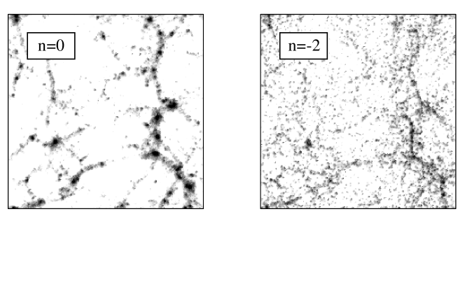
Figure 3: Slices through $N$-body simulations of different power spectra, using the same set of random phases for the modes in both cases. The slices are $1/15$ of the box in thickness, and density from 0.5 to 50 is log encoded. The box-scale power is the same in both cases, and produces much the same large-scale filamentary structure. However, the $n=0$ spectrum has much more small-scale power, and this manifests itself as far stronger clumping within the overall skeleton of the structure.

Despite these caveats, the results of $N$-body dynamics paint an impressive picture of the large-scale mass distribution. Consider figure 3, which shows slices through the computational density field for two particular sets of initial conditions, with different relative amplitudes of long and short wavelengths, but with the same amplitude for the modes with wavelengths equal to the side of the computational box. Although the small-scale ‘lumpiness’ is different, both display a similar large-scale network of filaments and voids – bearing a striking resemblance to the features seen in reality.

The state of the art in these calculations now routinely involves $10^{8}$ to $10^{9}$ particles, covering box sizes from the minimum necessary so that the box-scale modes do not saturate ($\sim 100{\,h^{-1}\,\rm Mpc}$) to effectively the entire observable universe (e.g. Evrard et al. 2002). The resolution available in the smaller boxes is sufficient that the nonlinear evolution of collisionless mass distributions is now effectively a solved problem, and nonlinear clustering statistics for model universes of practical interest can be measured to a few % precision (e.g. Jenkins et al. 1998). Further improvements in these sort of calculations are unlikely to be of practical importance, because of the need to include the evolution of the baryonic component, which makes up around 20% of the total matter density. The history of the gas is immensely complex, since it is strongly influenced by feedback of energy from the stars that form within it. The limitation of our modelling of such processes lies not so much in simple numerical aspects such as resolution, but in the simplifying assumptions used to treat processes that occur on scales very far below the resolution of any simulation. See e.g. Katz, Weinberg & Hernquist (1996); Pearce et al. (2001).

4 Statistics of cosmological density fields

Having discussed the main elements of the theory of cosmological structure formation, we now turn to the statistical treatment of data – which is how theory and observation will be confronted. The density perturbation field, $\delta$, inhabits a universe that is isotropic and homogeneous in its large-scale properties, suggesting that the statistical properties of $\delta$ should also be homogeneous. This statement sounds contradictory, and yet it makes perfect sense if there exists an ensemble of universes. The concept of an ensemble is used every time we apply probability theory to an event such as tossing a coin: we imagine an infinite sequence of repeated trials, half of which result in heads, half in tails. The analogy of coin tossing in cosmology is that the density at a given point in space will have different values in each member of the ensemble, with some overall variance $\langle\delta^{2}\rangle$ between members of the ensemble. Statistical homogeneity of the $\delta$ field then means that this variance must be independent of position. The actual field found in a given member of the ensemble is a realization of the statistical process.

There are two problems with this line of argument: (i) we have no evidence that the ensemble exists; (ii) in any case, we only get to observe one realization, so how is the variance $\langle\delta^{2}\rangle$ to be measured? The first objection applies to coin tossing, and may be evaded if we understand the physics that generates the statistical process – we only need to imagine tossing the coin many times, and we do not actually need to perform the exercise. The best that can be done in answering the second objection is to look at widely separated parts of space, since the $\delta$ fields there should be causally unconnected; this is therefore as good as taking measurements from two different member of the ensemble. In other words, if we measure the variance $\langle\delta^{2}\rangle$ by averaging over a sufficiently large volume, the results would be expected to approach the true ensemble variance, and the averaging operator $\langle\cdots\rangle$ is often used without being specific about which kind of average is intended. Fields that satisfy this property, whereby

$$\rm{volume\ average}\quad\leftrightarrow\quad{\rm ensemble\ average}$$ (72)

are termed ergodic. Giving a formal proof of ergodicity for a random process is not always easy (Adler 1981); in cosmology it is perhaps best regarded as a common-sense axiom.

4.1 Fourier analysis of density fluctuations

It is often convenient to consider building up a general field by the superposition of many modes. For a flat comoving geometry, the natural tool for achieving this is via Fourier analysis. For other models, plane waves are not a complete set and one should use instead the eigenfunctions of the wave equation in a curved space. Normally this complication is neglected: even in an open universe, the difference only matters on scales of order the present-day horizon.

How do we make a Fourier expansion of the density field in an infinite universe? If the field were periodic within some box of side $L$, then we would just have a sum over wave modes:

$$F({\bf x})=\sum F_{\bf k}e^{-i{\bf k\cdot x}}.$$ (73)

The requirement of periodicity restricts the allowed wavenumbers to harmonic boundary conditions

$$k_{x}=n\;{2\pi\over L},\;\quad n=1,2\cdots,$$ (74)

with similar expressions for $k_{y}$ and $k_{z}$. Now, if we let the box become arbitrarily large, then the sum will go over to an integral that incorporates the density of states in $k$-space, exactly as in statistical mechanics; this is how the general idea of the Fourier transform is derived. The Fourier relations in $n$ dimensions are thus

  $${F(x)} {{}=\left({L\over 2\pi}\right)^{n}\int F_{k}(k)\exp\bigl{(}-i{\bf k\cdot x}\bigr{)}\;d^{n}k} {F_{k}(k)} {{}=\left({1\over L}\right)^{n}\int F(x)\exp\bigl{(}i{\bf k\cdot x}\bigr{)}\;d^{n}x.}$$   (75)

One advantage of this particular Fourier convention is that the definition of convolution involves just a simple volume average, with no gratuitous factors of $(2\pi)^{-1/2}$:

$$f*g\equiv{1\over L^{n}}\int f({\bf x-y})g({\bf y})d^{n}y.$$ (76)

Although one can make all the manipulations on density fields that follow using either the integral or sum formulations, it is usually easier to use the sum. This saves having to introduce $\delta$-functions in $k$-space. For example, if we have $f=\sum f_{k}\exp(-ikx)$, the obvious way to extract $f_{k}$ is via $f_{k}=(1/L)\int f\exp(ikx)\;dx$: because of the harmonic boundary conditions, all oscillatory terms in the sum integrate to zero, leaving only $f_{k}$ to be integrated from 0 to $L$. There is less chance of committing errors of factors of $2\pi$ in this way than considering $f=(L/2\pi)\int f_{k}\exp(-ikx)\;dk$ and then using $\int\exp[i(k-K)x]\;dx=2\pi\delta_{\rm\scriptscriptstyle D}(k-K)$.

Correlation functions and power spectra  As an immediate example of the Fourier machinery in action, consider the important quantity

$${\xi({\bf r})\equiv\left\langle\delta({\bf x})\delta({\bf x+r})\right\rangle,}$$ (77)

which is the autocorrelation function of the density field – usually referred to simply as the correlation function. The angle brackets indicate an averaging over the normalization volume $V$. Now express $\delta$ as a sum and note that $\delta$ is real, so that we can replace one of the two $\delta$’s by its complex conjugate, obtaining

$$\xi=\left\langle\sum_{\bf k}\sum_{\bf k^{\prime}}\delta_{\bf k}\delta^{*}_{\bf k^{\prime}}e^{i{\bf(k^{\prime}-k)\cdot x}}e^{-i{\bf k\cdot r}}\right\rangle.$$ (78)

Alternatively, this sum can be obtained without replacing $\langle\delta\delta\rangle$ by $\langle\delta\delta^{*}\rangle$, from the relation between modes with opposite wavevectors that holds for any real field: $\delta_{\bf k}(-{\bf k})=\delta^{*}_{\bf k}({\bf k})$. Now, by the periodic boundary conditions, all the cross terms with $\bf k^{\prime}\neq k$ average to zero. Expressing the remaining sum as an integral, we have

$${\xi({\bf r})={V\over(2\pi)^{3}}\int|\delta_{\bf k}|^{2}e^{-i{\bf k\cdot r}}d^{3}k.}$$ (79)

In short, the correlation function is the Fourier transform of the power spectrum. This relation has been obtained by volume averaging, so it applies to the specific mode amplitudes and correlation function measured in any given realization of the density field. Taking ensemble averages of each side, the relation clearly also holds for the ensemble average power and correlations – which are really the quantities that cosmological studies aim to measure. We shall hereafter often use the alternative notation

$${P(k)\equiv\langle|\delta_{k}|^{2}\rangle}$$ (80)

for the ensemble-average power (although this only applies for a Fourier series with discrete modes). The distinction between the ensemble average and the actual power measured in a realization is clarified below in the section on Gaussian fields.

In an isotropic universe, the density perturbation spectrum cannot contain a preferred direction, and so we must have an isotropic power spectrum: $\langle|\delta_{\bf k}|^{2}({\bf k})\rangle=|\delta_{k}|^{2}(k)$. The angular part of the $k$-space integral can therefore be performed immediately: introduce spherical polars with the polar axis along $\bf k$, and use the reality of $\xi$ so that $e^{-i{\bf k\cdot x}}\rightarrow\cos(kr\cos\theta)$. In three dimensions, this yields

$$\xi(r)={V\over(2\pi)^{3}}\int P(k)\,{\sin kr\over kr}\,4\pi k^{2}\;dk.$$ (81)

The 2D analogue of this formula is

$$\xi(r)={A\over(2\pi)^{2}}\int P(k)\,J_{0}(kr)\,2\pi k\;dk.$$ (82)

We shall usually express the power spectrum in dimensionless form, as the variance per $\ln k$ ($\Delta^{2}(k)=d\langle\delta^{2}\rangle/d\ln k\propto k^{3}P[k]$):

$${\Delta^{2}(k)\equiv{V\over(2\pi)^{3}}\,4\pi k^{3}\,P(k)={2\over\pi}k^{3}\int_{0}^{\infty}\xi(r)\,{\sin kr\over kr}\,r^{2}\,dr.}$$ (83)

This gives a more easily visualizable meaning to the power spectrum than does the quantity $VP(k)$, which has dimensions of volume: $\Delta^{2}(k)=1$ means that there are order-unity density fluctuations from modes in the logarithmic bin around wavenumber $k$. $\Delta^{2}(k)$ is therefore the natural choice for a Fourier-space counterpart to the dimensionless quantity $\xi(r)$.

Power-law spectra  The above shows that the power spectrum is a central quantity in cosmology, but how can we predict its functional form? For decades, this was thought to be impossible, and so a minimal set of assumptions was investigated. In the absence of a physical theory, we should not assume that the spectrum contains any preferred length scale, otherwise we should then be compelled to explain this feature. Consequently, the spectrum must be a featureless power law:

$${\left\langle|\delta_{k}|^{2}\right\rangle\propto k^{n}}$$ (84)

The index $n$ governs the balance between large- and small-scale power. The meaning of different values of $n$ can be seen by imagining the results of filtering the density field by passing over it a box of some characteristic comoving size $x$ and averaging the density over the box. This will filter out waves with $k\mathrel{\lower 2.58334pt\hbox{$\buildrel{\textstyle>}\over{\scriptstyle\sim}$}}1/x$, leaving a variance $\langle\delta^{2}\rangle\propto\int_{0}^{1/x}k^{n}4\pi k^{2}dk\propto x^{-(n+3)}$. Hence, in terms of a mass $M\propto x^{3}$, we have

$$\delta_{\rm rms}\propto M^{-(n+3)/6}.$$ (85)

Similarly, a power-law spectrum implies a power-law correlation function. If $\xi(r)=(r/r_{0})^{-\gamma}$, with $\gamma=n+3$, the corresponding 3D power spectrum is

$$\Delta^{2}(k)={2\over\pi}\,(kr_{0})^{\gamma}\,\Gamma(2-\gamma)\,\sin{(2-\gamma)\pi\over 2}\equiv\beta(kr_{0})^{\gamma}$$ (86)

($=0.903(kr_{0})^{1.8}$ if $\gamma=1.8$). This expression is only valid for $n<0$ ($\gamma<3$); for larger values of $n$, $\xi$ must become negative at large $r$ (because $P(0)$ must vanish, implying $\int_{0}^{\infty}\xi(r)\,r^{2}\,dr=0$). A cutoff in the spectrum at large $k$ is needed to obtain physically sensible results.

What general constraints can we set on the value of $n$? Asymptotic homogeneity clearly requires $n>-3$. An upper limit of $n<4$ comes from an argument due to Zeldovich. Suppose we begin with a totally uniform matter distribution and then group it into discrete chunks as uniformly as possible. It can be shown that conservation of momentum in this process means that we cannot create a power spectrum that goes to zero at small wavelengths more rapidly than $\delta_{k}\propto k^{2}$. Thus, discreteness of matter produces the minimal spectrum, $n=4$. More plausible alternatives lie between these extremes. The value $n=0$ corresponds to white noise, the same power at all wavelengths. This is also known as the Poisson power spectrum, because it corresponds to fluctuations between different cells that scale as $1/\sqrt{M_{\rm cell}}$. A density field created by throwing down a large number of point masses at random would therefore consist of white noise. Particles placed at random within cells, one per cell, create an $n=2$ spectrum on large scales.

Practical spectra in cosmology, conversely, have negative effective values of $n$ over a large range of wavenumber. For many years, the data on the galaxy correlation function were consistent with a single power law:

$${\xi_{g}(r)\simeq\left({r\over 5{\,h^{-1}\,\rm Mpc}}\right)^{-1.8}\quad\quad\left(1\mathrel{\lower 2.58334pt\hbox{$\buildrel{\textstyle<}\over{\scriptstyle\sim}$}}\xi\mathrel{\lower 2.58334pt\hbox{$\buildrel{\textstyle<}\over{\scriptstyle\sim}$}}10^{4}\right);}$$ (87)

see Peebles (1980), Davis & Peebles (1983). This corresponds to $n\simeq-1.2$. By contrast with the above examples, large-scale structure is ‘real’, rather than reflecting the low-$k$ Fourier coefficients of some small-scale process.

The Zeldovich spectrum  Most important of all is the scale-invariant spectrum, which corresponds to the value $n=1$, i.e. $\Delta^{2}\propto k^{4}$. To see how the name arises, consider a perturbation $\Phi$ in the gravitational potential:

$$\nabla^{2}\Phi=4\pi G\rho_{0}\delta\quad\Rightarrow\quad\Phi_{k}=-4\pi G\rho_{0}\delta_{k}/k^{2}.$$ (88)

The two powers of $k$ pulled down by $\nabla^{2}$ mean that, if $\Delta^{2}\propto k^{4}$ for the power spectrum of density fluctuations, then $\Delta^{2}_{\Phi}$ is a constant. Since potential perturbations govern the flatness of spacetime, this says that the scale-invariant spectrum corresponds to a metric that is a fractal: spacetime has the same degree of ‘wrinkliness’ on each resolution scale. The total curvature fluctuations diverge, but only logarithmically at either extreme of wavelength.

Another way of looking at this spectrum is in terms of perturbation growth balancing the scale dependence of $\delta$: $\delta\propto x^{-(n+3)/2}$. We know that $\delta$ viewed on a given comoving scale will increase with the size of the horizon: $\delta\propto r_{\rm\scriptscriptstyle H}^{2}$. At an arbitrary time, though, the only natural length provided by the universe (in the absence of non-gravitational effects) is the horizon itself:

$$\delta(r_{\rm\scriptscriptstyle H})\propto r_{\rm\scriptscriptstyle H}^{2}r_{\rm\scriptscriptstyle H}^{-(n+3)/2}=r_{\rm\scriptscriptstyle H}^{-(n-1)/2}.$$ (89)

Thus, if $n=1$, the growth of both $r_{\rm\scriptscriptstyle H}$ and $\delta$ with time cancels out so that the universe always looks the same when viewed on the scale of the horizon; such a universe is self-similar in the sense of always appearing the same under the magnification of cosmological expansion. This spectrum is often known as the Zeldovich spectrum (sometimes hyphenated with Harrison and Peebles, who invented it independently).

The generic nature of the scale-invariant spectrum makes it difficult to use as a test, since many theories may be expected to have a chance of yielding something like a fractal spacetime. The interesting aspect to focus on is therefore where theory predicts deviations from this rule. Inflation is an interesting case, since the horizon-scale amplitude is expected to change logarithmically with scale in simple models (Hawking 1982):

$$\delta_{\rm\scriptscriptstyle H}\propto[-\ln(kr_{\rm\scriptscriptstyle H}^{\rm infl})]^{\alpha},$$ (90)

where $\alpha$ is a constant of order unity that depends on the inflationary potential ($\alpha=2$ for $V(\phi)=m^{2}\phi^{2}/2$, for example). Since the proper horizon scale at the end of inflation cannot be infinitely small ($a^{\rm infl}r_{\rm\scriptscriptstyle H}^{\rm infl}>\ell_{\rm Planck}$), we see that $\delta_{\rm\scriptscriptstyle H}$ should vary by a small but definite amount over the range of scales that can be probed by the CMB and large-scale structure (a change by a factor 1.07 between $k=0.1{\,h\,\rm Mpc^{-1}}$ and $10^{-3}{\,h\,\rm Mpc^{-1}}$, taking $\alpha=1$, $r_{\rm\scriptscriptstyle H}^{\rm infl}=\ell_{\rm Planck}/a^{\rm infl}$ and $a^{\rm infl}\simeq 2.73/T_{\rm Planck}$, so that $r_{\rm\scriptscriptstyle H}^{\rm infl}=10^{-3.08}{\rm m}$). This is pretty close to scale-invariance, but shows that small amounts of tilt are potentially observable if sufficiently accurate observations can be made.

4.2 CDM models for structure formation

The elements discussed so far assemble into the $\Lambda$CDM cosmological model, which is the simplest possibility that is consistent with current evidence. The overall matter power spectrum is written dimensionlessly as the logarithmic contribution to the fractional density variance, $\sigma^{2}$:

$$\Delta^{2}(k)={d\sigma^{2}\over d\ln k}\propto k^{3}|\delta_{k}|^{2}\propto k^{3+n},$$ (91)

which undergoes linear growth

$$\delta_{k}(a)=\delta_{k}(a_{0})\;\left[{D(a)\over D(a_{0})}\right]\;T_{k},$$ (92)

where the linear growth law is $D(a)=a\,g[\Omega(a)]$ in the matter era, and the growth suppression factor for a density parameter $\Omega_{m}\neq 1$ is

$${g(\Omega_{m})\simeq\frac{5}{2}\Omega_{m}\left[\Omega_{m}^{4/7}-\Omega_{v}+(1+\frac{1}{2}\Omega_{m})(1+\frac{1}{70}\Omega_{v})\right]^{-1}.}$$ (93)

The transfer function $T_{k}$ depends on the dark-matter content as discussed earlier, in particular displaying a horizon-scale break at $k\simeq 0.06(\Omega_{m}h)^{-1}{\,h\,\rm Mpc^{-1}}$. Weak oscillatory features are also expected if the universe has a significant baryon content. Eisenstein & Hu (1998) give an accurate fitting formula that describes these wiggles. This detailed fit of the CDM spectrum is to be preferred to the older notation in which the spectrum was described by the zero-baryon form, but with an effective value of $\Omega_{m}h$ that allowed for the main effects of the baryon content:

$$(\Omega_{m}h)_{\rm eff}\equiv\Gamma=\Omega_{m}h\,\exp\bigl{[}-\Omega_{b}(1+\sqrt{2h}/\Omega)\bigr{]}$$ (94)

(Sugiyama 1995).

5 Comparison with 2dFGRS data

5.1 Survey overview

The largest dataset for which a thorough comparison with the above picture has been made is the 2dF Galaxy Redshift Survey (2dFGRS). This survey was designed around the 2dF multi-fibre spectrograph on the Anglo-Australian Telescope, which is capable of observing up to 400 objects simultaneously over a 2 degree diameter field of view. For details of the instrument and its performance see http://www.aao.gov.au/2df/, and also Lewis et al. (2002). The source catalogue for the survey is a revised and extended version of the APM galaxy catalogue (Maddox et al. 1990a,b,c); this includes over 5 million galaxies down to $b_{\rm\scriptscriptstyle J}=20.5$ in both north and south Galactic hemispheres over a region of almost $10^{4}\,{\rm deg}^{2}$. The $b_{\rm\scriptscriptstyle J}$ magnitude system is related to the Johnson–Cousins system by $b_{\rm\scriptscriptstyle J}=B-0.304(B-V)$, where the colour term is estimated from comparison with the SDSS Early Data Release (Stoughton et al. 2002).

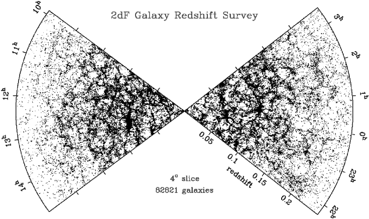
Figure 4: The distribution of galaxies in part of the 2dFGRS: slices $4^{\circ}$ thick, centred at declination $-2.5^{\circ}$ in the NGP and $-27.5^{\circ}$ in the SGP. This magnificently detailed image of large-scale structure provides the basis for measuring the shape of the primordial fluctuation spectrum and hence constraining the matter content of the universe.

The 2dFGRS geometry consists of two contiguous declination strips, plus 100 random 2-degree fields. One strip is in the southern Galactic hemisphere and covers approximately 75^∘$\times$15^∘ centred close to the SGP at ($\alpha,\delta$)=($01^{h}$,$-30^{\circ}$); the other strip is in the northern Galactic hemisphere and covers $75^{\circ}\times 7.5^{\circ}$ centred at ($\alpha,\delta$)=($12.5^{h}$,$+0^{\circ}$). The 100 random fields are spread uniformly over the 7000 deg² region of the APM catalogue in the southern Galactic hemisphere. The sample is limited to be brighter than an extinction-corrected magnitude of $b_{\rm\scriptscriptstyle J}=19.45$ (using the extinction maps of Schlegel et al. 1998). This limit gives a good match between the density on the sky of galaxies and 2dF fibres.

After an extensive period of commissioning of the 2dF instrument, 2dFGRS observing began in earnest in May 1997, and terminated in April 2002. In total, observations were made of 899 fields, yielding redshifts and identifications for 232,529 galaxies, 13976 stars and 172 QSOs, at an overall completeness of 93%. The galaxy redshifts are assigned a quality flag from 1 to 5, where the probability of error is highest at low $Q$. Most analyses are restricted to $Q\geq 3$ galaxies, of which there are currently 221,496. An interim data release took place in July 2001, consisting of approximately 100,000 galaxies (see Colless et al. 2001 for details). A public release of the full photometric and spectroscopic database is scheduled for July 2003. The completed 2dFGRS yields a striking view of the galaxy distribution over large cosmological volumes. This is illustrated in figure 5, which shows the projection of a subset of the galaxies in the northern and southern strips onto $(\alpha,z)$ slices. This picture is the culmination of decades of effort in the investigation of large-scale structure, and we are fortunate to have this detailed view for the first time.

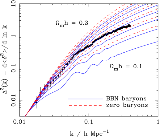
Figure 5: The 2dFGRS redshift-space dimensionless power spectrum, $\Delta^{2}(k)$, estimated according to the FKP procedure. The solid points with error bars show the power estimate. The window function correlates the results at different $k$ values, and also distorts the large-scale shape of the power spectrum An approximate correction for the latter effect has been applied. The solid and dashed lines show various CDM models, all assuming $n=1$. For the case with non-negligible baryon content, a big-bang nucleosynthesis value of $\Omega_{b}h^{2}=0.02$ is assumed, together with $h=0.7$. A good fit is clearly obtained for $\Omega_{m}h\simeq 0.2$. Note that the observed power at large $k$ will be boosted by nonlinear effects, but damped by small-scale random peculiar velocities. It appears that these two effects very nearly cancel, but model fitting is generally performed only at $k<0.15{\,h\,\rm Mpc^{-1}}$ in order to avoid these complications.

5.2 The 2dFGRS power spectrum and CDM models

Perhaps the key aim of the 2dFGRS was to perform an accurate measurement of the 3D clustering power spectrum, in order to improve on the APM result, which was deduced by deprojection of angular clustering (Baugh & Efstathiou 1993, 1994). The results of this direct estimation of the 3D power spectrum are shown in figure 5 (Percival et al. 2001). This power-spectrum estimate uses the FFT-based approach of Feldman, Kaiser & Peacock (1994), and needs to be interpreted with care. Firstly, it is a raw redshift-space estimate, so that the power beyond $k\simeq 0.2{\,h\,\rm Mpc^{-1}}$ is severely damped by smearing due to peculiar velocities, as well as being affected by nonlinear evolution. Finally, the FKP estimator yields the true power convolved with the window function. This modifies the power significantly on large scales (roughly a 20% correction). An approximate correction for this has been made in figure 5.

Figure 6: Likelihood contours for the best-fit linear CDM fit to the 2dFGRS power spectrum over the region $0.02<k<0.15$. Contours are plotted at the usual positions for one-parameter confidence of 68%, and two-parameter confidence of 68%, 95% and 99% (i.e. $-2\ln({\cal L}/{\cal L_{\rm max}})=1,2.3,6.0,9.2$). We have marginalized over the missing free parameters ($h$ and the power spectrum amplitude). A prior on $h$ of $h=0.7\pm 10\%$ was assumed. This result is compared to estimates from X-ray cluster analysis (Evrard 1997) and big-bang nucleosynthesis (Burles et al. 2001). The second panel shows the 2dFGRS data compared with the two preferred models from the Maximum Likelihood fits convolved with the window function (solid lines). The unconvolved models are also shown (dashed lines). The $\Omega_{m}h\simeq 0.6$, $\Omega_{b}/\Omega_{m}=0.42$, $h=0.7$ model has the higher bump at $k\simeq 0.05{\,h\,\rm Mpc^{-1}}$. The smoother $\Omega_{m}h\simeq 0.20$, $\Omega_{b}/\Omega_{m}=0.15$, $h=0.7$ model is a better fit to the data because of the overall shape. A preliminary analysis of the complete final 2dFGRS sample yields a slightly smoother spectrum than the results shown here (from Percival et al. 2001), so that the high-baryon solution becomes disfavoured.

The fundamental assumption is that, on large scales, linear biasing applies, so that the nonlinear galaxy power spectrum in redshift space has a shape identical to that of linear theory in real space. This assumption is valid for $k<0.15{\,h\,\rm Mpc^{-1}}$; the detailed justification comes from analyzing realistic mock data derived from $N$-body simulations (Cole et al. 1998). The free parameters in fitting CDM models are thus the primordial spectral index, $n$, the Hubble parameter, $h$, the total matter density, $\Omega_{m}$, and the baryon fraction, $\Omega_{b}/\Omega_{m}$. Note that the vacuum energy does not enter. Initially, we show results assuming $n=1$; this assumption is relaxed later.

An accurate model comparison requires the full covariance matrix of the data, because the convolving effect of the window function causes the power at adjacent $k$ values to be correlated. This covariance matrix was estimated by applying the survey window to a library of Gaussian realisations of linear density fields, and checked against a set of mock catalogues. It is now possible to explore the space of CDM models, and likelihood contours in $\Omega_{b}/\Omega_{m}$ versus $\Omega_{m}h$ are shown in figure 6. At each point in this surface we have marginalized by integrating the likelihood surface over the two free parameters, $h$ and the power spectrum amplitude. We have added a Gaussian prior $h=0.7\pm 10\%$, representing external constraints such as the HST key project (Freedman et al. 2001); this has only a minor effect on the results.

Figure 6 shows that there is a degeneracy between $\Omega_{m}h$ and the baryonic fraction $\Omega_{b}/\Omega_{m}$. However, there are two local maxima in the likelihood, one with $\Omega_{m}h\simeq 0.2$ and $\sim 20\%$ baryons, plus a secondary solution $\Omega_{m}h\simeq 0.6$ and $\sim 40\%$ baryons. The high-density model can be rejected through a variety of arguments, and the preferred solution is

$$\Omega_{m}h=0.20\pm 0.03;\quad\quad\Omega_{b}/\Omega_{m}=0.15\pm 0.07.$$ (95)

The 2dFGRS data are compared to the best-fit linear power spectra convolved with the window function in figure 6. The low-density model fits the overall shape of the spectrum with relatively small ‘wiggles’, while the solution at $\Omega_{m}h\simeq 0.6$ provides a better fit to the bump at $k\simeq 0.065{\,h\,\rm Mpc^{-1}}$, but fits the overall shape less well. A preliminary analysis of $P(k)$ from the full final dataset shows that $P(k)$ becomes smoother: the high-baryon solution becomes disfavoured, and the uncertainties narrow slightly around the lower-density solution: $\Omega_{m}h=0.18\pm 0.02$; $\Omega_{b}/\Omega_{m}=0.17\pm 0.06$. The lack of large-amplitude oscillatory features in the power spectrum is one general reason for believing that the universe is dominated by collisionless nonbaryonic matter. In detail, the constraints on the collisional nature of dark matter are weak, since all we require is that the effective sound speed for modes of 100-Mpc wavelength is less than about $0.1c$. Nevertheless, if a pure-baryon model is ruled out, the next simplest alternative would arguably be to introduce a weakly-interacting relic particle, so there is at least circumstantial evidence in this direction from the power spectrum.

It is interesting to compare these conclusions with other constraints. These are shown on figure 6, again assuming $h=0.7\pm 10\%$. Estimates of the Deuterium to Hydrogen ratio in QSO spectra combined big-bang nucleosynthesis theory predict $\Omega_{b}h^{2}=0.020\pm 0.001$ (Burles et al. 2001), which translates to the shown locus of $f_{b}$ vs $\Omega_{m}h$. X-ray cluster analysis yields a baryon fraction $\Omega_{b}/\Omega_{m}=0.127\pm 0.017$ (Evrard 1997) which is within $1\sigma$ of our value. These loci intersect very close to our preferred model.

Perhaps the main point to emphasise here is that the 2dFGRS results are not greatly sensitive to the assumed tilt of the primordial spectrum. As discussed below, CMB data show that $n=1$ is a very good approximation; in any case, very substantial tilts ($n\simeq 0.8$) are required to alter the conclusions significantly.

Figure 7: The power spectra of red galaxies (filled circles) and blue galaxies (open circles), divided at photographic $B-R=0.85$. The shapes are strikingly similar, and the square root of the ratio yields the right-hand panel: the relative bias in redshift space of red and blue galaxies. The error bars are obtained by a jack-knife analysis. The relative bias is consistent with a constant value of 1.4 over the range used for fitting of the power-spectrum data ($0.015<k<0.15{\,h\,\rm Mpc^{-1}}$).

5.3 Robustness of results

The main residual worry about accepting the above conclusions is probably whether the assumption of linear bias can really be valid. In general, concentration towards higher-density regions both raises the amplitude of clustering, but also steepens the correlations, so that bias is largest on small scales, as discussed below. We need to be clear of the regime in which the bias depends on scale.

One way in which this issue can be studied is to consider subsamples with very different degrees of bias. Colour information has recently been added to the 2dFGRS database using SuperCosmos scans of the UKST red plates (Hambly et al. 2001), and a division at rest-frame photographic $B-R=0.85$ nicely separates ellipticals from spirals. Figure 7 shows the power spectra for the 2dFGRS divided in this way. The shapes are almost identical (perhaps not so surprising, since the cosmic variance effects are closely correlated in these co-spatial samples). However, what is impressive is that the relative bias is almost precisely independent of scale, even though the red subset is rather strongly biased relative to the blue subset (relative $b\simeq 1.4$). This provides some reassurance that the large-scale $P(k)$ reflects the underlying properties of the dark matter, rather than depending on the particular class of galaxies used to measure it.

6 Relation of galaxies and dark matter

6.1 History and general aspects of bias

In order to make full use of the cosmological information encoded in large-scale structure, it is essential to understand the relation between the number density of galaxies and the mass density field. It was first appreciated during the 1980s that these two fields need not be strictly proportional. Until this time, the general assumption was that galaxies ‘trace the mass’. Since the mass density is a continuous field and galaxies are point events, the approach is to postulate a Poisson clustering hypothesis, in which the number of galaxies in a given volume is a Poisson sampling from a fictitious number-density field that is proportional to the mass. Thus within a volume $V$,

$$\langle N_{g}(V)\rangle\propto M(V).$$ (96)

With allowance for this discrete sampling, the observed numbers of galaxies, $N_{g}$, would give an unbiased estimate of the mass in a given region.

The first motivation for considering that galaxies might in fact be biased mass tracers came from attempts to reconcile the $\Omega_{m}=1$ Einstein–de Sitter model with observations. Although $M/L$ ratios in rich clusters argued for dark matter, as first shown by Zwicky (1933), typical blue values of $M/L\simeq 300h$ implied only $\Omega_{m}\simeq 0.2$ if they were taken to be universal. Those who argued that the value $\Omega_{m}=1$ was more natural (a greatly increased camp after the advent of inflation) were therefore forced to postulate that the efficiency of galaxy formation was enhanced in dense environments: biased galaxy formation.

We can note immediately that a consequence of this bias in density will be to affect the velocity statistics of galaxies relative to dark matter. Both galaxies and dark-matter particles follow orbits in the overall gravitational potential well of a cluster; if the galaxies are to be more strongly concentrated towards the centre, they must clearly have smaller velocities than the dark matter. This is the phenomenon known as velocity bias (Carlberg, Couchman & Thomas 1990).

An argument for bias at the opposite extreme of density arose through the discovery of large voids in the galaxy distribution (Kirshner et al. 1981). There was a reluctance to believe that such vast regions could be truly devoid of matter – although this was at a time before the discovery of large-scale velocity fields. This tendency was given further stimulus through the work of Davis, Efstathiou, Frenk & White (1985), who were the first to calculate $N$-body models of the detailed nonlinear structure arising in CDM-dominated universes. Since the CDM spectrum curves slowly between effective indices of $n=-3$ and $n=1$, the correlation function steepens with time. There is therefore a unique epoch when $\xi$ will have the observed slope of $-1.8$. Davis et al. identified this epoch as the present and then noted that, for $\Omega_{m}=1$, it implied a rather low amplitude of fluctuations: $r_{0}=1.3h^{-2}$ Mpc. An independent argument for this low amplitude came from the size of the peculiar velocities in CDM models: if the spectrum was given an amplitude corresponding to the $\sigma_{8}\simeq 1$ seen in the galaxy distribution, the pairwise dispersion was $\sigma_{p}\simeq 1000$ – $1500{\,\rm km\,s^{-1}}$, around 3 times the observed value. What seemed to be required was a galaxy correlation function that was an amplified version of that for mass. This was exactly the phenomenon analysed for Abell clusters by Kaiser (1984), and thus was born the idea of high-peak bias: bright galaxies form only at the sites of high peaks in the initial density field. This was developed in some analytical detail by Bardeen et al. (1986), and was implemented in the simulations of Davis et al. (1985).

Figure 8: The high-peak bias model. If we decompose a density field into a fluctuating component on galaxy scales, together with a long-wavelength ‘swell’ (shown dashed), then those regions of density that lie above a threshold in density of $\nu$ times the rms will be strongly clustered. If proto-objects are presumed to form at the sites of these high peaks (shaded, and indicated by arrows), then this is a population with Lagrangian bias – i.e. a non-uniform spatial distribution even prior to dynamical evolution of the density field. The key question is the physical origin of the threshold; for massive objects such as clusters, the requirement of collapse by the present imposes a threshold of $\nu\mathrel{\lower 2.58334pt\hbox{$\buildrel{\textstyle>}\over{\scriptstyle\sim}$}}2$. For galaxies, there will be no bias without additional mechanisms to cause star formation to favour those objects that collapse first.

As shown below, the high-peak model produces a linear amplification of large-wavelength modes. This is likely to be a general feature of other models for bias, so it is useful to introduce the linear bias parameter:

$${\left({\delta\rho\over\rho}\right)_{\rm galaxies}=b\,\left({\delta\rho\over\rho}\right)_{\rm mass}.}$$ (97)

This seems a reasonable assumption when $\delta\rho/\rho\ll 1$, although it leaves open the question of how the effective value of $b$ would be expected to change on nonlinear scales. Galaxy clustering on large scales therefore allows us to determine mass fluctuations only if we know the value of $b$. When we observe large-scale galaxy clustering, we are only measuring $b^{2}\xi_{\rm mass}(r)$ or $b^{2}\Delta^{2}_{\rm mass}(k)$.

Later studies of bias concentrated on general models. A fruitful assumption is that bias is local, so that the number density of galaxies is some nonlinear function of the mass density

$$n_{g}({\bf r})=f[\rho_{m}({\bf r})].$$ (98)

Coles (1993) proved the powerful result that, whatever the function $f$ may be, the quantity

$$b(r)\equiv\sqrt{\xi_{g}(r)/\xi_{m}(r)}$$ (99)

had to show a monotonic dependence on scale, provided the mass density field had Gaussian statistics. An interesting concrete example of this is provided by the lognormal density field (Coles & Jones 1991); this is generated by exponentiation of a Gaussian field:

$$1+\delta_{\rm\scriptscriptstyle LN}=\exp(\delta_{\rm\scriptscriptstyle G}-\sigma^{2}/2),$$ (100)

where $\sigma^{2}$ is the total variance in the Gaussian field. These authors argue that this analytical form is a reasonable approximation to the exact nonlinear evolution of the mass density distribution function, preventing the unphysical values $\delta<-1$. This non-Gaussian model is built upon an underlying Gaussian field, so the joint distribution of the density at $n$ points is still known. This means that the correlations are simple enough to calculate, the result being

$$\xi_{\rm\scriptscriptstyle LN}=\exp(\xi_{\rm\scriptscriptstyle G})-1.$$ (101)

This says that $\xi$ on large scales is unaltered by nonlinearities in this model; they only add extra small-scale correlations. Using the lognormal model as a hypothetical nonlinear density field, we can now introduce bias. A nonlinear local transformation $\rho_{g}\propto\rho_{\rm\scriptscriptstyle LN}^{b}$ then gives a correlation function $1+\xi_{g}=(1+\xi_{\rm\scriptscriptstyle LN})^{b^{2}}$ (Mann, Peacock & Heavens 1998). The linear bias parameter is $b$, but the correlations steepen on small scales, as expected for Coles’ result.

In reality, bias is unlikely to be completely causal, and this has led some workers to explore stochastic bias models, in which

$$n_{g}=f(\rho_{m})+\epsilon,$$ (102)

where $\epsilon$ is a random field that is uncorrelated with the mass density (Pen 1998; Dekel & Lahav 1999). This means we need to consider not only the bias parameter defined via the ratio of correlation functions, but also the correlation coefficient, $r$, between galaxies and mass:

$$b^{2}={\langle\delta_{g}\delta_{g}^{\prime}\rangle\over\langle\delta_{m}\delta_{m}^{\prime}\rangle}\quad\quad r^{2}={\langle\delta_{g}\delta_{m}^{\prime}\rangle^{2}\over\langle\delta_{g}\delta_{g}^{\prime}\rangle\langle\delta_{m}\delta_{m}^{\prime}\rangle}.$$ (103)

Although truly stochastic effects are possible in galaxy formation, a relation of the above form is expected when the galaxy and mass densities are filtered on some scale (as they always are, in practice). Just averaging a galaxy density that is a nonlinear function of the mass will lead to some scatter when comparing with the averaged mass field; a scatter will also arise when the relation between mass and light is non-local, however, and this may be the dominant effect.

6.2 The peak-background split

We now consider the central mechanism of biased clustering, in which a rare high density fluctuation, corresponding to a massive object, collapses sooner if it lies in a region of large-scale overdensity. This ‘helping hand’ from the long-wavelength modes means that overdense regions contain an enhanced abundance of massive objects with respect to the mean, so that these systems display enhanced clustering. The basic mechanism can be immediately understood via the diagram in figure 8; it was first clearly analysed by Kaiser (1984) in the context of rich clusters of galaxies. What Kaiser did not do was consider the degree of bias that applies to more typical objects; the generalization to consider objects of any mass was made by Cole & Kaiser (1989; see also Mo & White 1996 and Sheth et al. 2001).

The key ingredient of this analysis is the mass function of dark-matter haloes. The universe fragments into virialized systems such that $f(M)\,dM$ is the number density of haloes in the mass range $dM$; conservation of mass requires that $\int M\,f(M)\,dM=\rho_{0}$. A convenient related dimensionless quantity is therefore the multiplicity function, $M^{2}f(M)/\rho_{0}$, which gives the fraction of the mass of the universe contained in haloes of a unit range in $\ln M$. The simplest analyses of the mass function rest on the concept of a density threshold: collapse to a virialized object is deemed to have occurred where linear-theory $\delta$ averaged over a box containing mass $M$ reaches some critical value $\delta_{c}$. Generally, we shall assume the value $\delta_{c}=1.686$ appropriate for spherical collapse in an Einstein–de Sitter universe. Now imagine that this situation is perturbed, by adding some constant shift $\epsilon$ to the density perturbations over some large region. The effect of this is to perturb the threshold: fluctuations now only need to reach $\delta=\delta_{c}-\epsilon$ in order to achieve collapse. The number density is therefore modulated:

$$f\rightarrow f-{df\over d\delta_{c}}\,\epsilon.$$ (104)

This gives a bias in the number density of haloes in Lagrangian space: $\delta f/f=b_{\rm\scriptscriptstyle L}\epsilon$, where the Lagrangian bias is

$$b_{\rm\scriptscriptstyle L}=-{d\ln f\over d\delta_{c}}.$$ (105)

In addition to this modulation of the halo properties, the large-scale disturbance will move haloes closer together where $\epsilon$ is large, giving a density contrast of $1+\epsilon$. If $\epsilon\ll 1$, the overall fractional density contrast of haloes is therefore the sum of the dynamical and statistical effects: $\delta_{\rm halo}=\epsilon+b_{\rm\scriptscriptstyle L}\epsilon$. The overall bias in Eulerian space ($b=\delta_{\rm halo}/\epsilon$) is therefore

$$b=1-{d\ln f\over d\delta_{c}}.$$ (106)

Of course, the field $\epsilon$ can hardly be imposed by hand; instead, we make the peak-background split, in which $\delta$ is mentally decomposed into a small-scale and a large-scale component – which we identify with $\epsilon$. The scale above which the large-scale component is defined does not matter so long as it lies between the sizes of collapsed systems and the scales at which we wish to measure correlations.

To apply this, we need an explicit expression for the mass function. The simplest alternative is the original expression of Press & Schechter (1974), which can be written in terms of the parameter $\nu=\delta_{c}/\sigma(M)$:

$$M^{2}f(M)/\rho_{0}=\sqrt{2\over\pi}\,\nu\,\exp\left(-{\nu^{2}\over 2}\right).$$ (107)

We now use $d/d\delta_{c}=\sigma(M)^{-1}(d/d\nu)=(\nu/\delta_{c})(d/d\nu)$, since $M$ is not affected by the threshold change, which yields

$${b(\nu)=1+{\nu^{2}-1\over\delta_{c}}.}$$ (108)

This says that $M^{*}$ haloes are unbiased, low-mass haloes are antibiased and high-mass haloes are positively biased, eventually reaching the $b=\nu/\sigma$ value expected for high peaks. The corresponding expression can readily be deduced for more accurate fitting formulae for the mass function, such as that of Sheth & Tormen (1999):

$$M^{2}f(M)/\rho_{0}=0.21617[1+(\sqrt{2}/\nu^{2})^{0.3}]\,\nu\,\exp[-\nu^{2}/(2\sqrt{2})].$$ (109)

We can now understand the observation that Abell clusters are much more strongly clustered than galaxies in general: regions of large-scale overdensity contain systematically more high-mass haloes than expected if the haloes traced the mass. This phenomenon was dubbed natural bias by White et al. (1987). However, applying the idea to galaxies is not straightforward: we have shown that enhanced clustering is only expected for massive fluctuations with $\sigma\mathrel{\lower 2.58334pt\hbox{$\buildrel{\textstyle<}\over{\scriptstyle\sim}$}}1$, but galaxies at $z=0$ fail this criterion. The high-peak idea applies will at high redshift, where massive galaxies are still assembling, but today there has been time for galaxy-scale haloes to collapse in all environments. The large bias that should exist at high redshifts is erased as the mass fluctuations grow: if the Lagrangian component to the biased density field is kept unaltered, then the present-day bias will tend to unity as

$$b(\nu)=1+{\nu^{2}-1\over(1+z_{f})\delta_{c}}.$$ (110)

(Fry 1986; Tegmark & Peebles 1998). Strong galaxy bias at $z=0$ therefore requires some form of selection that locates present-day galaxies preferentially in the rarer haloes with $M>M^{*}$ (Kauffmann, Nusser & Steinmetz 1997).

This dilemma forced the introduction of the idea of high-peak bias: bright galaxies form only at the sites of high peaks in the initial density field (Bardeen et al. 1986; Davis et al. 1985). This idea is commonly, but incorrectly, attributed to Kaiser (1984), but it needs an extra ingredient, namely a non-gravitational threshold. Attempts were therefore made to argue that the first generation of objects could propagate disruptive signals, causing neighbours in low-density regions to be ‘still-born’. It is then possible to construct models (e.g. Bower et al. 1993) in which the large-scale modulation of the galaxy density is entirely non-gravitational in nature. However, it turned out to be hard to make such mechanisms operate: the energetics and required scale of the phenomenon are very large (Rees 1985; Dekel & Rees 1987). These difficulties were only removed when the standard model became a low-density universe, in which the dynamical argument for high galaxy bias no longer applied.

Figure 9: The correlation length for clusters of galaxies, $r_{0}$, as a function of mean intercluster separation, $d_{c}$, taken from Colberg et al. (2000). Results are shown for $\tau$CDM (open squares) and $\Lambda$CDM (filled squares) simulations. The predictions of Sheth et al. (2001) are shown as solid lines. Also shown are data from the APM cluster catalogue (open triangles), taken from Croft et al. (1997).

6.3 Observations of biased clustering

As indicated above, the first strong indications of biased clustering came from measurements of the correlation function of Abell clusters, which showed a far greater amplitude than for galaxies in general (Klypin & Kopylov 1983; Bahcall & Soneira 1983). Following Kaiser (1984), Cole & Kaiser (1989) etc., our explanation for this is that massive haloes show clustering that is an increasing function of mass. This is illustrated in figure 9, which shows that the rarest and most rich clusters (as measured by the intercluster separation) have the highest clustering, and that the trend is in agreement with the theoretical predictions.

Figure 10: (a) The correlation length in real space as a function of absolute magnitude. The solid line shows the predictions of the semi-analytic model of Benson et al. (2001), computed in a series of overlapping bins, each $0.5$ magnitudes wide. The dotted curves show an estimate of the errors on this prediction, including the relevant sample variance for the survey volume. (b) The real space correlation length estimated combining the NGP and SGP (filled circles). The open symbols show a selection of recent data from other studies.

Because galaxy halo masses are less extreme, it is not so clear a priori that any trend of this sort should be expected for galaxies. However, our empirical knowledge of luminosity functions and morphological segregation did argue for an effect. It has been clear for many years that elliptical galaxies display a higher correlation amplitude than spirals (Davis & Geller 1976), and this makes sense in terms of the preference of ellipticals for cluster environments. Since ellipticals are also more luminous on average than spirals, some trend with luminosity is to be expected, but the challenge is to detect it. For a number of years, the existence of any effect was controversial (e.g. Loveday et al. 1995; Benoist et al. 1996), but Norberg et al. (2001) were able to use the 2dFGRS to demonstrate very clearly that the effect existed, as shown in Figure 10. The results can be described by a linear dependence of effective bias parameter on luminosity:

$$b/b^{*}=0.85+0.15\,(L/L^{*}),$$ (111)

and the scale-length of the real-space correlation function for $L^{*}$ galaxies is approximately $r_{0}=4.8{\,h^{-1}\,\rm Mpc}$. Finally, with spectral classifications, it is possible to measure the dependence of clustering both on luminosity and on spectral type, to see to what extent morphological segregation is responsible for this result. Norberg et al. (2002) show that, in fact, the principal effect seems to be with luminosity: $\xi(r)$ increases with $L$ for all spectral types.

Finally, we can look at high-redshift clustering. At high enough redshift, $M^{*}$ is of order a galaxy mass and galaxies could be strongly biased relative to the mass at that time. Indeed, there is good evidence that this is the case. Steidel et al. (1997) have used the Lyman-limit technique to select galaxies around redshifts $2.5\mathrel{\lower 2.58334pt\hbox{$\buildrel{\textstyle<}\over{\scriptstyle\sim}$}}z\mathrel{\lower 2.58334pt\hbox{$\buildrel{\textstyle<}\over{\scriptstyle\sim}$}}3.5$ and found their distribution to be highly inhomogeneous. The apparent value of $\sigma_{8}$ for these objects is of order unity (Adelberger et al. 1998), whereas the present value of $\sigma_{8}\simeq 0.8$ should have evolved to about 0.26 at these redshifts (for $\Omega_{m}=0.3$, $k=0$). This suggests a bias parameter of $b\simeq 4$, or $\nu\simeq 2.5$, which requires a halo mass of about $10^{12.1}h^{-1}M_{\odot}$ for concordance $\Lambda$CDM. The masses of these high-redshift galaxies can be estimated directly through their stellar masses, which are typically $10^{10}h^{-2}M_{\odot}$ (Papovich, Dickinson & Ferguson 2001), and thus only 1% of what is required in order to explain the clustering. This is an unreasonably small baryon fraction, so the correct explanation is more plausibly that each $10^{12}h^{-1}M_{\odot}$ halo at $z=3$ contains a number of Lyman-break galaxies. This theme is pursued below.

6.4 Scale dependence of bias

The Poisson clustering hypothesis would propose that galaxies are simply a dilute sampling of the mass field. If this were a correct hypothesis, no CDM universe would be acceptable, since the correlation functions for these models differ from the observed galaxy correlations in a complicated scale-dependent fashion (e.g. Klypin, Primack & Holtzman 1996; Peacock 1997; Jenkins et al. 1998).

Figure 11: The correlation function of galaxies in the semianalytical simulation of an LCDM universe by Benson et al. (2000a). Although the nonlinear correlations of the mass show a characteristic convex bulge at separations around 1 Mpc, the galaxy data follow a power law which thus is antibiased on these small scales. The simulation is successful at reproducing this trend.

For a few years, this failure of CDM models to match the shape of the galaxy power spectrum was seen as a serious problem, but this was eventually resolved by more detailed theoretical predictions for galaxy clustering. Two approaches are being followed in this regard. The brute-force method is to perform $N$-body simulations in which the evolution of both collisionless dark matter and dissipative gas is followed, with the physical state of the gas (i.e. its ability to cool) being used as a cue to insert star formation. The stars in turn are allowed to feed energy back into the gas, simulating the effects of mass loss and supernovae. This determines the star formation history of a given halo, and its appearance can be predicted using spectral synthesis codes. This is challenging, but starting to be feasible with current computing power (Pearce et al. 2001). The alternative is ‘semianalytic’ modelling, in which the merging history of dark-matter haloes is treated via the extended Press-Schechter theory (Bond et al. 1991), and the location of galaxies within haloes is estimated using dynamical-friction arguments (e.g. Kauffmann et al. 1993, 1999; Cole et al. 1994, 2000; Somerville & Primack 1999; van Kampen, Jimenez & Peacock 1999; Benson et al. 2000a,b).

Both these approaches have yielded similar conclusions, and shown how CDM models can match the galaxy data: specifically, the low-density flat $\Lambda$CDM model that is favoured on other grounds can yield a correlation function that is close to a single power law over $1000\mathrel{\lower 2.58334pt\hbox{$\buildrel{\textstyle>}\over{\scriptstyle\sim}$}}\xi\mathrel{\lower 2.58334pt\hbox{$\buildrel{\textstyle>}\over{\scriptstyle\sim}$}}1$, even though the mass correlations show a marked curvature over this range (Pearce et al. 1999; 2001; Benson et al. 2000a; see figure 11). These results are impressive, yet it is frustrating to have a result of such fundamental importance emerge from a complicated calculational apparatus. There is thus some motivation for constructing a simpler heuristic model that captures the main processes at work in the full semianalytic models. The following section describes an approach of this sort (Peacock & Smith 2000; Seljak 2000; Cooray & Sheth 2002).

6.5 The halo model – I: mass

The formation of galaxies must be a non-local process to some extent, and the modern paradigm was introduced by White & Rees (1978): galaxies form through the cooling of baryonic material in virialized haloes of dark matter. The virial radii of these systems are in excess of 0.1 Mpc, so there is the potential for large differences in the correlation properties of galaxies and dark matter on these scales. The ‘halo model’ addresses this by creating a density field in which dark-matter haloes are superimposed. The key feature that allows bias to be included is to encode all the complications of galaxy formation via the halo occupation number: the number of galaxies found above some luminosity threshold in a virialized halo of a given mass.

To some extent, this is a very old idea: one of the earliest suggested models for the galaxy correlation function was to consider a density field composed of randomly-placed independent clumps with some universal density profile (Neyman, Scott & Shane 1953; Peebles 1974). Since the clumps are placed at random (with number density $n$), the only excess neighbours to a given mass point arise from points in the same clump, and the correlation function is straightforward to compute in principle. For the case where the clumps have a power-law density profile,

$$\rho=nBr^{-\epsilon},$$ (112)

truncated at $r=R$, the small-$r$ behaviour of the correlation function is $\xi\propto r^{3-2\epsilon}$, provided $3/2<\epsilon<3$. For smaller values of $\epsilon$, $\xi(r)$ tends to a constant as $r\rightarrow 0$. In the isothermal $\epsilon=2$ case, the correlation function for $r\ll R$ is

$$\xi(r)={\pi^{2}B\over 4rR}={\pi N\over 16rR^{2}n},$$ (113)

where $N$ is the total number of particles per clump (Peebles 1974).

Figure 12: A comparison of various possible density profiles for virialized haloes. The dotted line is a singular isothermal sphere. The solid lines show haloes with formation redshifts of 0 and 5 according to NFW ($\Omega=1$) and M99.

The general result is that the correlation function is less steep at small $r$ than the clump density profile, which is inevitable because an autocorrelation function involves convolving the density field with itself. A long-standing problem for this model is therefore that the predicted correlation function is much flatter than is observed for galaxies: $\xi\propto r^{-1.8}$ is the canonical slope, apparently requiring clumps with very steep density profiles, $\epsilon=2.4$. This is not in agreement with the profiles of dark-matter haloes as ‘observed’ in numerical simulations.

Traditionally, virialized systems have been found by a criterion based on percolation (‘friends-of-friends’), such that the mean density is about 200 times the mean. Sometimes, the criterion is taken as a density of 200 times the critical value. We shall use the former definition:

$$r_{v}=\left({3M\over 800\pi\rho_{b}}\right)^{1/3}.$$ (114)

Thus $r_{v}$ is related to the Lagrangian radius containing the mass via $r_{v}=R/200^{1/3}$. Of course, the density contrast used to define the boundary of an object is somewhat arbitrary. Fortunately, much of the mass resides at smaller radii, near a ‘core radius’. These core radii are relatively insensitive to the exact definition of virial radius.

The simplest model for the density structure of the virialized system is the singular isothermal sphere: $\rho=\sigma_{v}^{2}/(2\pi Gr^{2})$, or

$$\rho/\rho_{b}={200\over 3y^{2}};\quad(y<1);\quad y\equiv r/r_{v}.$$ (115)

A more realistic alternative is the profile proposed by Navarro, Frenk & White (1996; NFW):

$$\rho/\rho_{b}={\Delta_{c}\over y(1+y)^{2}};\quad(r<r_{v});\quad y\equiv r/r_{c}.$$ (116)

The parameter $\Delta_{c}$ is related to the core radius and the virial radius via

$$\Delta_{c}={200c^{3}/3\over\ln(1+c)-c/(1+c)};\quad c\equiv r_{v}/r_{c}$$ (117)

(we change symbol from NFW’s $\delta_{c}$ to avoid confusion with the linear-theory density threshold for collapse, and also because our definition of density is relative to the mean, rather than the critical density). NFW showed that $\Delta_{c}$ is related to collapse redshift via

$$\Delta_{c}\simeq 3000(1+z_{c})^{3},$$ (118)

An advantage of the definition of virial radius used here is that $\Delta_{c}$ is independent of $\Omega$ (for given $z_{c}$), whereas NFW’s $\delta_{c}$ is $\propto\Omega$.

The above equations determine the concentration, $c=r_{v}/r_{c}$ implicitly, hence in principle giving $r_{c}$ in terms of $r_{v}$ once $\Delta_{c}$ is known. NFW give a procedure for determining $z_{c}$. A simplified argument would suggest a typical formation era determined by $D(z_{c})=1/\nu$, where $D$ is the linear-theory growth factor between $z=z_{c}$ and the present, and $\nu$ is the dimensionless fluctuation amplitude corresponding to the system in units of the rms: $\nu\equiv\delta_{c}/\sigma(M)$, where $\delta_{c}\simeq 1.686$. For very massive systems with $\nu\gg 1$, only rare fluctuations have collapsed by the present, so $z_{c}$ is close to zero. This suggests the interpolation formula

$$D(z_{c})=1+1/\nu;$$ (119)

The NFW formula is actually of this form, except that the $1/\nu$ term is multiplied by a spectrum-dependent coefficient of order unity. It has been claimed by Moore et al. (1999; M99) that the NFW density profile is in error at small $r$. M99 proposed the alternative form

$$\rho/\rho_{b}={\Delta_{c}\over y^{3/2}(1+y^{3/2})};\quad(r<r_{v});\quad y\equiv r/r_{c}.$$ (120)

It is straightforward to use this in place of the NFW profile.

We now compute the power spectrum for the halo model. Start by distributing point seeds throughout the universe with number density $n$, in which case the power spectrum of the resulting density field is just shot noise:

$$\Delta^{2}(k)={4\pi\over n}\,\left({k\over 2\pi}\right)^{3}.$$ (121)

Here, we use a dimensionless notation for the power spectrum: $\Delta^{2}$ is the contribution to the fractional density variance per unit interval of $\ln k$. In the convention of Peebles (1980), this is

$$\Delta^{2}(k)\equiv{{\rm d}\sigma^{2}\over{\rm d}\ln k}={V\over(2\pi)^{3}}\,4\pi\,k^{3}\,|\delta_{k}|^{2}$$ (122)

($V$ being a normalization volume), and the relation to the correlation function is

$$\xi(r)=\int\Delta^{2}(k)\;{dk\over k}\;{\sin kr\over kr}.$$ (123)

The density field for a distribution of clumps is produced by convolution of the initial field of delta-functions, so the power spectrum is simply modified by the squared Fourier transform of the clump density profile:

$$\Delta^{2}(k)={4\pi\over n}\,\left({k\over 2\pi}\right)^{3}\;|W_{k}|^{2},$$ (124)

where

$$W_{k}={\int\rho(r)\,{\displaystyle\sin kr\over\displaystyle kr}\,4\pi\,r^{2}\;dr\over\int\rho(r)\,4\pi\,r^{2}\;dr}.$$ (125)

For a practical calculation, we should also use the fact that hierarchical models are expected to contain a distribution of masses of clumps. If we use the notation $f(M)\,dM$ to denote the number density of haloes in the mass range $dM$, the effective number density in the shot noise formula becomes

$${1\over n_{\rm eff}}={\int M^{2}\,f(M)\,dM\over\left[\,\int M\,f(M)\,dM\,\right]^{2}}.$$ (126)

The window function also depends on mass, so the overall power spectrum is

$$\Delta^{2}_{\rm halo}(k)=4\pi\,\left({k\over 2\pi}\right)^{3}\;{\int M^{2}\,|W_{k}(M)|^{2}\,f(M)\,dM\over\left[\,\int M\,f(M)\,dM\,\right]^{2}}.$$ (127)

The normalization term $\int M\,f(M)\,dM$ just gives the total background density, $\rho_{b}$, so there is only a single numerical integral to perform. Using this model, it is then possible to calculate the correlations of the nonlinear density field, neglecting only the large-scale correlations in halo positions. The power spectrum determined in this way is shown in figure 13, and turns out to agree very well with the exact nonlinear result on small and intermediate scales. The lesson here is that a good deal of the nonlinear correlations of the dark matter field can be understood as a distribution of random clumps, provided these are given the correct distribution of masses and mass-dependent density profiles.

Figure 13: The decomposition of the mass power spectrum according to the halo model, for the flat $\Omega_{m}=0.3$, $\Gamma=0.2$, $\sigma_{8}=0.8$ case. The dashed line shows linear theory, and the open circles show the predicted 1-halo contribution. Adding in linear theory to produce the correct large-scale clustering yields the solid points. The full lines show the contribution of different mass ranges to the 1-halo term: bins of width a factor 10 in width, starting at $10^{10}-10^{11}h^{-1}M_{\odot}$ and ending at $10^{15}-10^{16}h^{-1}M_{\odot}$. The more massive haloes have larger virial radii and hence filter the power spectrum on progressively larger scales. The majority of the quasilinear power is contributed by the haloes near the peak in the mass function at $10^{14}-10^{15}h^{-1}M_{\odot}$.

So far, we have ignored any spatial correlations in the halo positions. A simple guess for amending this is to add the linear power spectrum to the power generated by the halo structure:

$$\Delta^{2}_{\rm tot}=\Delta^{2}_{\rm halo}+\Delta^{2}_{\rm linear}.$$ (128)

The justification for this is that the extra small-scale power introduced by nonlinear evolution is associated with the internal structure of the haloes. In practice, this model works extremely well, giving an almost perfect description of the power spectrum on all scales. This is a novel way of looking at the features in the nonlinear spectrum, particularly the steep rise between $k\simeq 0.5{\,h\,\rm Mpc^{-1}}$ and $k\simeq 5{\,h\,\rm Mpc^{-1}}$, and the flattening on smaller scales. According to the ideas presented here, the flat small-scale spectrum arises because haloes have central density profiles rising as $r^{-1.5}$, but not much faster. The sharp fall in power at smaller $k$ reflects the cutoff at the virial radii of the haloes that dominate the correlation signal.

It might be objected that this model is still not completely realistic, since we have treated haloes as smooth objects and ignored any substructure. At one time, it was generally believed that collisionless evolution would lead to the destruction of galaxy-scale haloes when they are absorbed into the creation of a larger-scale nonlinear system such as a group or cluster. However, it turns out that this ‘overmerging problem’ was only an artefact of inadequate resolution (see e.g. van Kampen 2000). When a simulation is carried out with $\sim 10^{6}$ particles in a rich cluster, the cores of galaxy-scale haloes can still be identified after many crossing times (Ghigna et al. 1998). This substructure must have some effect on the correlations of the density field, and indeed Valageas (1999) has argued that the high-order correlations of the density field seen in $N$-body simulations are inconsistent with a model where the density file is composed of smooth virialized haloes. Nevertheless, substructure seems to be unimportant at the level of two-point correlations.

The existence of substructure is important for the obvious next step of this work, which is to try to understand galaxy correlations within the current framework. It is clear that the galaxy-scale substructure in large dark-matter haloes defines directly where luminous galaxies will be found, giving hope that the main features of galaxy formation can be understood principally in terms of the dark-matter distribution. Indeed, if catalogues of these ‘sub-haloes’ are created within a cosmological-sized simulation, their correlation function is known to differ from that of the mass (e.g. Klypin et al. 1999; Ma 1999). The model of a density field consisting of smooth haloes may therefore be a useful description of the galaxy field, and this is explored in the following section.

6.6 The Halo model – II: biased galaxy populations

In relating the distribution of galaxies to that of the mass, there are two distinct ways in which a degree of bias is inevitable:

(1)         Halo occupation numbers. For low-mass haloes, the probability of obtaining an $L^{*}$ galaxy must fall to zero. For haloes with mass above this lower limit, the number of galaxies will in general not scale linearly with halo mass.

(2)         Nonlocality. Galaxies can orbit within their host haloes, so the probability of forming a galaxy depends on the overall halo properties, not just the density at a point. Also, the galaxies can occupy special places within the haloes: for a halo containing only one galaxy, the galaxy will clearly mark the halo centre. In general, we will assume one central galaxy and a number of satellites.

The first mechanism leads to large-scale bias, because large-scale halo correlations depend on mass, and are some biased multiple of the mass power spectrum: $\Delta^{2}_{h}=b^{2}(M)\Delta^{2}$. As discussed earlier, the linear bias parameter for a given class of haloes, $b(M)$, depends on the rareness of the fluctuation and the rms of the underlying field:

$$b=1+{\nu^{2}-1\over\nu\sigma}=1+{\nu^{2}-1\over\delta_{c}}$$ (129)

(Kaiser 1984; Cole & Kaiser 1989; Mo & White 1996), where $\nu=\delta_{c}/\sigma$, and $\sigma^{2}$ is the fractional mass variance at the redshift of interest. This formula is not perfectly accurate, but the deviations may be traced to the fact that the Press-Schechter formula for the number density of haloes (which is assumed in deriving the bias) is itself systematically in error; see Sheth & Tormen (1999).

If we do not wish to assume that the number of galaxies in a halo of mass $M$ is strictly proportional to $M$, we are in effect giving haloes a mass-dependent weight, as was first considered by Jing, Mo & Börner (1998). A simple but instructive model for this is

$$w(M)=\cases{0\quad&($M<M_{c}$)\cr(M/M_{c})^{\alpha-1}\quad&($M>M_{c}$)\cr}$$ (130)

A model in which mass traces light would have $M_{c}\rightarrow 0$ and $\alpha=1$. We will show below that, empirically, we should choose $\alpha<1$.

The bias formula applies to haloes of a given $\nu$, i.e. of a given mass, so the effect of mass-dependent weights is

$$b_{\rm tot}=1+{\int_{\nu}^{\infty}b(\nu)\,w(\nu)\,{dF\over d\nu}\;d\nu\over\int_{\nu}^{\infty}w(\nu)\,{dF\over d\nu}\;d\nu,}$$ (131)

Where $F(>\nu)$ is the fraction of the mass in haloes exceeding a given $\nu$; $dF/d\nu\propto\exp(-\nu^{2}/2)$ according to Press-Schechter theory. The total model for the galaxy power spectrum is then

$$\Delta^{2}_{g}=\left\langle\Delta^{2}_{\rm halo}\right\rangle+b_{\rm tot}^{2}\Delta^{2}_{\rm lin}$$ (132)

where

$$\left\langle\Delta^{2}_{\rm halo}(k)\right\rangle=4\pi\,\left({k\over 2\pi}\right)^{3}\;{\int M^{2}\,w^{2}(M)\,|W_{k}(M)|^{2}\,f(M)\,dM\over\left[\,\int M\,w(M)\,f(M)\,dM\,\right]^{2}}.$$ (133)

The key ingredient needed to make this machinery work is the occupation number, which in principle needs to be calculated via a detailed numerical model of galaxy formation. However, for a given assumed background cosmology, the answer may be determined empirically. Galaxy redshift surveys have been analyzed via grouping algorithms similar to the ‘friends-of-friends’ method widely employed to find virialized clumps in $N$-body simulations. With an appropriate correction for the survey limiting magnitude, the observed number of galaxies in a group can be converted to an estimate of the total stellar luminosity in a group. This allows a determination of the All Galaxy System (AGS) luminosity function: the distribution of virialized clumps of galaxies as a function of their total luminosity, from small systems like the Local Group to rich Abell clusters.

Figure 14: The empirical luminosity–mass relation required to reconcile the observed AGS luminosity function with two variants of CDM. $L^{*}$ is the characteristic luminosity in the AGS luminosity function ($L^{*}=7.6\times 10^{10}h^{-2}L_{\odot}$). Note the rather flat slope around $M=10^{13}$ to $10^{14}h^{-1}M_{\odot}$, especially for $\Lambda$CDM.

Figure 15: The power spectrum predicted for the halo model, for the flat $\Omega_{m}=0.3$, $\Gamma=0.2$, $\sigma_{8}=0.8$ case. The halo occupation numbers are predicted according to a simple two-parameter model, in which haloes are only included above some minimum value, $M_{\rm min}$, and receive a weight $\propto M^{\alpha}$. A model with ‘mass traces light’ would have $M_{\rm min}=0$ and $\alpha=1$. Motivated by the results on abundances of groups, we choose $\alpha=0.5$. Results are shown for $M_{\rm min}$ in the range $10^{10}$ (lowest) to $10^{12.5}h^{-1}M_{\odot}$ (highest). The mass power spectrum is shown as a dashed line (linear theory) and as points (nonlinear). The second panel shows the scale-dependent relative bias, i.e. the square root of the ratio between galaxy and mass power spectra. The dashed lines show the bias with respect to linear theory. The final panel shows the ratio to the canonical power-law spectrum; for $M_{\rm min}$ in the region of $10^{12}h^{-1}M_{\odot}$, the result is within a factor 2 of a perfect power law over a factor 300 in scale.

The AGS function for the CfA survey was investigated by Moore, Frenk & White (1993), who found that the result in blue light was well described by

$$d\phi=\phi^{*}\,\left[(L/L^{*})^{\beta}+(L/L^{*})^{\gamma}\right]^{-1}\;dL/L^{*},$$ (134)

where $\phi^{*}=0.00126h^{3}\rm Mpc^{-3}$, $\beta=1.34$, $\gamma=2.89$; the characteristic luminosity is $L^{*}=7.6\times 10^{10}h^{-2}L_{\odot}$. One notable feature of this function is that it is rather flat at low luminosities, in contrast to the mass function of dark-matter haloes (see Sheth & Tormen 1999). It is therefore clear that any fictitious galaxy catalogue generated by randomly sampling the mass is unlikely to be a good match to observation. The simplest cure for this deficiency is to assume that the stellar luminosity per virialized halo is a monotonic, but nonlinear, function of halo mass. The required luminosity–mass relation is then easily deduced by finding the luminosity at which the integrated AGS density $\Phi(>L)$ matches the integrated number density of haloes with mass $>M$. The result is shown in figure 14.

We can now calculate the halo-based galaxy power spectrum and use semi-realistic occupation numbers, $N$, as a function of mass. This is needs a little care at small numbers, however, since the number of haloes with occupation number unity affects the correlation properties. These haloes contribute no correlated pairs, so they simply dilute the signal from the haloes with $N\geq 2$. This means that we need in principle to use different weights for the large-scale bias and the halo term:

$$w_{i}={\left\langle N_{i}\right\rangle\over M}\quad\quad w_{i}={\left\langle N_{i}(N_{i}-1)\right\rangle^{1/2}\over M}$$ (135)

respectively (Seljak 2000). In practice, this correction has a rather small effect, provided the relation between $N$ and $M$ has no scatter. If, in contrast, the distribution of $N$ for given $M$ is assumed to obey a Poisson distribution, the small-scale clustering properties are strongly affected, and do not match the data well (Benson et al. 2000a). Finally, we need to put the galaxies in the correct location, as discussed above. If one galaxy always occupies the halo centre, with others acting as satellites, the small-scale correlations automatically follow the slope of the halo density profile, which keeps them steep. The results of this exercise are shown in figure 15. This shows that, depending on the range of halo masses chosen, the galaxies can be positively or negatively biased with respect to the mass, as expected. What is particularly interesting is that the shape of the galaxy spectrum is expected to differ from that of the mass. For an appropriate mass range, the galaxy power spectrum can be very close to a power law, which has been a long-standing puzzle to explain. Interestingly, the power-law should not be perfect; small deviations have long been suspected, and were confirmed by Hawkins et al. (2002) and Zehavi et al. (2003). The inflection is at a scale of $\sim 0.5{\,h\,\rm Mpc^{-1}}$, as expected from the halo model. Figure 15 also shows that the results of this simple model are encouragingly similar to the scale-dependent bias found in the detailed calculations of Benson et al. (2000a), shown in figure 11. There are thus grounds for optimism that we may be starting to attain a physical understanding of the origin of galaxy bias.

7 Anisotropies in the CMB

Despite the great progress in precise measurements of large-scale structure, we cannot achieve a complete specification of the cosmological model in this way alone. The vacuum energy is not probed, since this affects mainly the growth rate of structure – which is degenerate with bias evolution. The matter content is only constrained if we assume that $n=1$, and even then we only measure $\Omega_{m}$ if a value for $h$ is supplied. A more complete picture is obtained if we include data on clustering at much earlier times: the anisotropy of the microwave background, which reaches us from $z\simeq 1100$. In addition to breaking degeneracies, studies of this sort also test the basic gravitational instability theory – which will be seen to work very well indeed over this redshift range. This section briefly reviews the physics of CMB anisotropies, and presents recent data. For more details, see e.g. Hu & Dodelson (2002), or Dodelson (2003).

7.1 Anisotropy mechanisms

Fluctuations in the 2D temperature perturbation field are treated similarly to density fluctuations, except that the field is expanded in spherical harmonics, so modes of different scales are labelled by multipole number, $\ell$. Once again, we can define a ‘power per octave’ measure for the temperature fluctuations:

$${\mathcal{T}}^{2}(\ell)=\ell(\ell+1)C_{\ell}/2\pi;\quad\quad\left\langle(\delta T/T)^{2}\right\rangle=\sum_{\ell}(2\ell+1)\,C_{\ell}/4\pi,$$ (136)

where the $C_{\ell}$ are another common way of representing the power. Note that ${\mathcal{T}}^{2}(\ell)$ is a power per $\ln\ell$; the modern trend is often to plot CMB fluctuations with a linear scale for $\ell$ – in which case one should really use ${\mathcal{T}}^{2}(\ell)/\ell$.

We now list the mechanisms that cause primary anisotropies in the CMB (as opposed to secondary anisotropies, which are generated by scattering along the line of sight). There are three basic primary effects, illustrated in figure 16, which are important on respectively large, intermediate and small angular scales:

(1) Gravitational (Sachs–Wolfe) perturbations. Photons from high-density regions at last scattering have to climb out of potential wells, and are thus redshifted:

$${\delta T\over T}={\Phi\over c^{2}}.$$ (137)

(2) Intrinsic (adiabatic) perturbations. In high-density regions, the coupling of matter and radiation can compress the radiation also, giving a higher temperature:

$${\delta T\over T}={\delta(z_{\rm\scriptscriptstyle LS})\over 3},$$ (138)

(3) Velocity (Doppler) perturbations. The plasma has a non-zero velocity at recombination, which leads to Doppler shifts in frequency and hence brightness temperature:

$${\delta T\over T}={{\bf\delta v\cdot\hat{r}}\over c}.$$ (139)

To the above list should be added ‘tensor modes’: anisotropies due to a background of primordial gravitational waves, potentially generated during an inflationary era (see below).

There are in addition effects generated along the line of sight. One important effect is the integrated Sachs-Wolfe effect, which arises when the potential perturbations evolve:

$${\delta T\over T}=2\int{\dot{\Phi}\over c^{2}}\;dt.$$ (140)

This happens both at early times (because radiation is still important) and late times (because of $\Lambda$). Other effects are to do with the development of nonlinear structure, and are mainly on small scales (principally the Sunyaev–Zeldovich effect from IGM Comptonization). The exception is the effect of reionization; to a good approximation, this merely damps the fluctuations on all scales:

$${\delta T\over T}\quad\rightarrow\quad{\delta T\over T}\,\exp-\tau,$$ (141)

where the optical depth must exceed $\tau\simeq 0.04$, based on the highest-redshift quasars and the BBN baryon density. As we will see later, CMB polarization data have detected a signature consistent with $\tau=0.17\pm 0.04$, implying reionization at $z\simeq 20$.

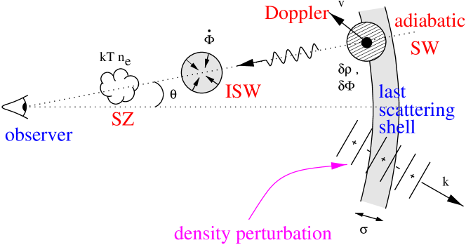
Figure 16: Illustrating the physical mechanisms that cause CMB anisotropies. The shaded arc on the right represents the last-scattering shell; an inhomogeneity on this shell affects the CMB through its potential, adiabatic and Doppler perturbations. Further perturbations are added along the line of sight by time-varying potentials (Rees–Sciama effect) and by electron scattering from hot gas (Sunyaev–Zeldovich effect). The density field at last scattering can be Fourier analysed into modes of wavevector ${\bf k}$. These spatial perturbation modes have a contribution that is in general damped by averaging over the shell of last scattering. Short-wavelength modes are more heavily affected (i) because more of them fit inside the scattering shell, and (ii) because their wavevectors point more nearly radially for a given projected wavelength.

7.2 Inflationary predictions

The most commonly-discussed mechanism for generating the inhomogeneities that act as the source for $\delta T/T$ is inflation. Of course, CMB anisotropies were calculated in largely the modern way well before inflation was ever considered, by Peebles & Yu (1970). The standard approach involves super-horizon fluctuations, which must be generated by some acausal process. Inflation achieves this – but we cannot claim that detection of super-horizon modes amounts to a proof of inflation. Rather, we need some more characteristic signature of the specific process used by inflation: amplified quantum fluctuations (see e.g. chapter 11 of Peacock 1999 or Liddle & Lyth 2000 for details).

In the simplest models, inflation is driven by a scalar field $\phi$, with a potential $V(\phi)$. As well as the characteristic energy density of inflation, $V$, this can be characterized by two parameters, $\epsilon$ & $\eta$, which are dimensionless versions of the first and second derivatives of $V$ with respect to $\phi$. In these terms, the inflationary predictions for the perturbation index is

$$n=1-6\epsilon+2\eta.$$ (142)

Since inflation continues while $\epsilon$ & $\eta$ are small, some tilt is expected ($|n-1|\sim 0.01$ to 0.05 in simple models).

The critical ingredient for testing inflation by making further predictions is the possibility that, in addition to scalar modes, the CMB could also be affected by gravitational waves (following the original insight of Starobinsky 1985). The relative amplitude of tensor and scalar contributions depended on the inflationary parameter $\epsilon$ alone:

$${C_{\ell}^{\rm\scriptscriptstyle T}\over C_{\ell}^{\rm\scriptscriptstyle S}}\simeq 12.4\epsilon\simeq 6(1-n_{\rm\scriptscriptstyle S}).$$ (143)

The second relation to the tilt is less general, as it assumes a polynomial-like potential, so that $\eta$ is related to $\epsilon$. For example, $V=\lambda\phi^{4}$ implies $n_{\rm\scriptscriptstyle S}\simeq 0.95$ and $C_{\ell}^{\rm\scriptscriptstyle T}/C_{\ell}^{\rm\scriptscriptstyle S}\simeq 0.3$. To be safe, we need one further observation, and this is potentially provided by the spectrum of $C_{\ell}^{\rm\scriptscriptstyle T}$. Suppose we write separate power-law index definitions for the scalar and tensor anisotropies:

$$C_{\ell}^{\rm\scriptscriptstyle S}\propto\ell^{n_{\rm\scriptscriptstyle S}-3},\quad\quad C_{\ell}^{\rm\scriptscriptstyle T}\propto\ell^{n_{\rm\scriptscriptstyle T}-3}.$$ (144)

For the scalar spectrum, we had $n_{\rm\scriptscriptstyle S}=n=1-6\epsilon+2\eta$; for the tensors, $n_{\rm\scriptscriptstyle T}=1-2\epsilon$ [although different definitions of $n_{\rm\scriptscriptstyle T}$ exist; the convention here is that $n=1$ always corresponds to a constant ${\mathcal{T}}^{2}(\ell)$]. Thus, a knowledge of $n_{\rm\scriptscriptstyle S}$, $n_{\rm\scriptscriptstyle T}$ and the scalar-to-tensor ratio would overdetermine the model and allow a genuine test of inflation.

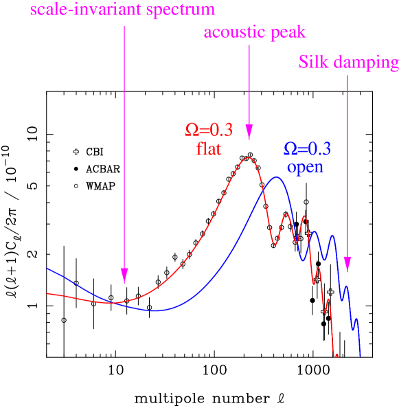
Figure 17: Angular power spectra ${\mathcal{T}}^{2}(\ell)=\ell(\ell+1)C_{\ell}/2\pi$ for the CMB, plotted against angular wavenumber $\ell$ in radians^-1. For references to the experimental data, see Spergel et al. (2003), Kuo et al. (2002) and Pearson et al. (2002). The two lines show model predictions for adiabatic scale-invariant CDM fluctuations, calculated using the ${\rm\scriptscriptstyle CMBFAST}$ package (Seljak & Zaldarriaga 1996). These have $(n,\Omega_{m},\Omega_{b},h)=(1,0.3,0.05,0.65)$ and have respectively $\Omega_{v}=1-\Omega_{m}$ (‘flat’) and $\Omega_{v}=0$ (‘open’). The main effect is that open models shift the peaks to the right, as discussed in the text.

7.3 Characteristic scales

The current data are contrasted with some CDM models in figure 17. The key feature that is picked out is the peak at $\ell\simeq 220$, together with harmonics of this scale at higher $\ell$. Beyond $\ell\simeq 1000$, the spectrum is clearly damped, in a manner consistent with the expected effects of photons diffusing away from baryons (Silk damping), plus smearing of modes with wavelength comparable to the thickness of the last-scattering shell. This last effect arises because recombination is not instantaneous, so the redshift of last scattering shows a scatter around the mean, with a thickness corresponding to approximately $\sigma_{r}=7(\Omega_{m}h^{2})^{-1/2}$ Mpc. On scales larger than this, we see essentially an instantaneous imprint of the pattern of potential perturbations and the acoustic baryon/photon oscillations.

The significance of the main acoustic peak scale is that it picks out the (sound) horizon at last scattering. The redshift of last scattering is almost independent of cosmological parameters at $z_{\rm\scriptscriptstyle LS}\simeq 1100$, although a more precise approximation is given in Appendix C of Hu & Sugiyama (1995). If we assume that the universe is matter dominated at last scattering, the horizon size is

$$D_{\rm\scriptscriptstyle H}^{\rm\scriptscriptstyle LS}=184\,(\Omega_{m}h^{2})^{-1/2}{\rm Mpc}.$$ (145)

The angle this subtends is given by dividing by the current size of the horizon (strictly, the comoving angular-diameter distance to $z_{\rm\scriptscriptstyle LS}$). Again, for a matter-dominated model, this is

$$D_{\rm\scriptscriptstyle H}=6000\,\Omega_{m}^{-1}\,h^{-1}{\rm Mpc}\quad\Rightarrow\quad\theta_{\rm\rm\scriptscriptstyle H}=D_{\rm\scriptscriptstyle H}^{\rm\scriptscriptstyle LS}/D_{\rm\scriptscriptstyle H}\propto\Omega_{m}^{0.5}.$$ (146)

This expression lies behind the common statement that the CMB data require a flat universe. Figure 17 shows that heavily open universes yield a main CMB peak at scales much smaller than the observed $\ell\simeq 220$, and these can be ruled out. Indeed, open models were disfavoured for this reason long before any useful data existed near the peak, simply because of strict upper limits at $\ell\simeq 1500$ (Bond & Efstathiou 1984). However, once a non-zero vacuum energy is allowed, the story becomes more complicated, and it turns out that large degrees of spatial curvature cannot be excluded using the CMB alone.

7.4 Evolution of CMB data

The pace of progress in CMB experiments has maintained an astonishing rate for a decade. Following the 1992 COBE detection of fluctuations, 5 years of effort yielded the unclear picture of the first panel in figure 18, in which of order 10 experiments gave only vague evidence for a peak in $\ell^{2}C_{\ell}$. By the year 2000, this had been transformed to a clear picture of a peak at $\ell\simeq 200$, although there was no model-independent evidence for higher harmonics. The present situation is much more satisfactory, with 3 peaks established in a way that does not require any knowledge of the CDM model.

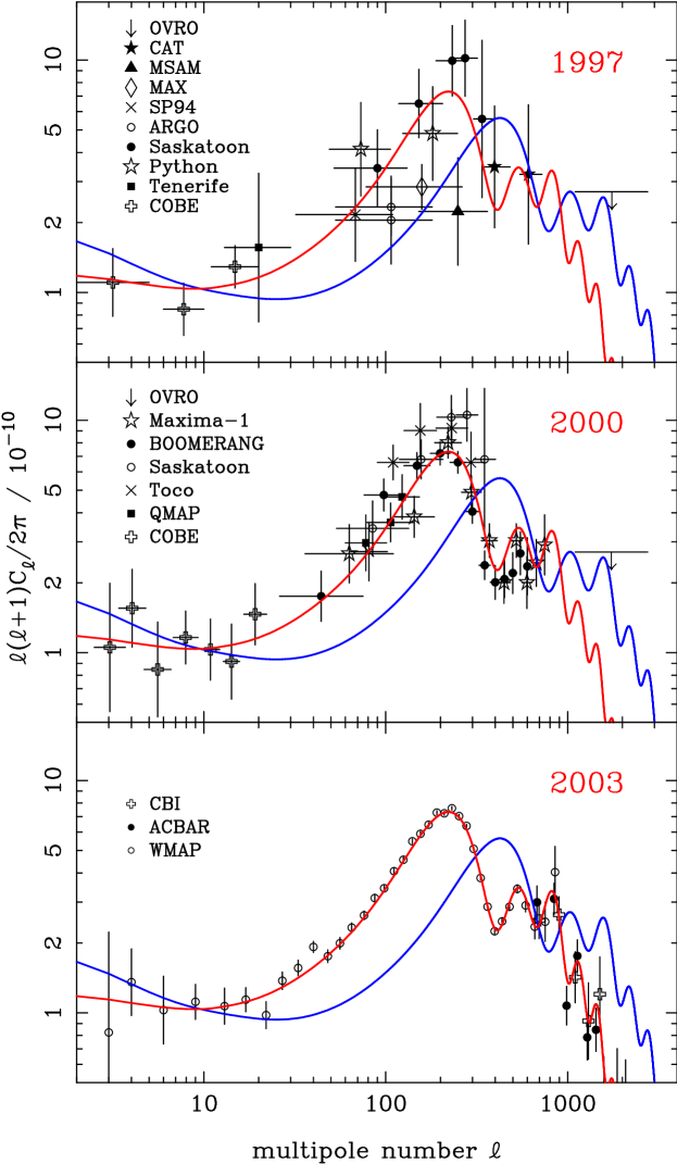
Figure 18: Dramatic change took place in CMB power spectrum measurements around the turn of the 21st century. Although some rise from the COBE level was arguably known even by 1997, a clear peak around $\ell\simeq 200$ only became established in 2000, whereas by 2003 definitive measurements of the spectrum at $\ell\mathrel{\lower 2.58334pt\hbox{$\buildrel{\textstyle<}\over{\scriptstyle\sim}$}}800$, limited mainly by cosmic variance, had been made by the WMAP satellite.

The WMAP results (Spergel et al. 2003) measure the power spectrum about as well as possible (i.e. hitting the limit of cosmic variance from a finite sky) up to the second peak. At smaller scales, however, there is still much scope for improvement, and the rate of advance is unlikely to drop in the future. The useful web page http://background.uchicago.edu/~whu/cmbex.html lists 14 ongoing experiments, as well as 19 completed ones.

8 Model degeneracies inherent in CMB data

8.1 Geometrical degeneracy

The normal argument for flatness from the CMB starts with the comoving horizon size at last scattering

$$D_{\rm\scriptscriptstyle LS}=\frac{2c}{\Omega_{m}^{1/2}H_{0}}\,(1+z_{\rm\scriptscriptstyle LS})^{-1/2}\simeq 184(\Omega_{m}h^{2})^{-1/2}\;{\rm Mpc}$$ (147)

and divides it by the present-day horizon size for a zero-$\Lambda$ universe,

$$D_{\rm\scriptscriptstyle H}=\frac{2c}{\Omega_{m}H_{0}},$$ (148)

to yield a main characteristic angle that scales as $\Omega_{m}^{1/2}$. Large curvature (i.e. low $\Omega_{m}$) is ruled out because the main peak in the CMB power spectrum is not seen at very small angles. However, introducing vacuum energy changes the conclusion. If we take a family of models with fixed initial perturbation spectra, fixed physical densities $\omega_{m}\equiv\Omega_{m}h^{2}$, $\omega_{b}\equiv\Omega_{b}h^{2}$, it is possible to vary both $\Omega_{v}$ and the curvature to keep a fixed value of the angular size distance to last scattering, so that the resulting CMB power spectra are identical. This degeneracy was analyzed comprehensively by Efstathiou & Bond (1999), and we now summarize the main results.

Figure 19: The geometrical degeneracy in the CMB means that models with fixed $\Omega_{m}h^{2}$ and $\Omega_{b}h^{2}$ can be made to look identical by varying the curvature against vacuum energy, while also varying the Hubble parameter. This degeneracy is illustrated here for the case $\omega_{m}\equiv\Omega_{m}h^{2}=0.2$. Models along a given line are equivalent from a CMB point of view; corresponding lines in the upper and lower panels have the same line style. Note that supplying external information about $h$ breaks the degeneracy. This figure assumes scalar fluctuations only; allowing tensor modes introduces additional degeneracies – mainly between the tensor fraction and tilt.

The usual expression for the comoving angular-diameter distance is

  $${R_{0}S_{k}(r)=} {{}{c\over H_{0}}|1-\Omega|^{-1/2}\quad\times} {{}S_{k}\left[\int_{0}^{z}\!\!{|1-\Omega|^{1/2}\;dz^{\prime}\over\sqrt{(1-\Omega)(1+z^{\prime})^{2}+\Omega_{v}+\Omega_{m}(1+z^{\prime})^{3}}}\right],}$$   (149)

where $\Omega=\Omega_{m}+\Omega_{v}$. Defining $\omega_{i}\equiv\Omega_{i}h^{2}$, this can be rewritten in a way that has no explicit $h$ dependence:

$$R_{0}S_{k}(r)={3000\,{\rm Mpc}\over|\omega_{k}|^{1/2}}S_{k}\left[\int_{0}^{z}\!\!{|\omega_{k}|^{1/2}\;dz^{\prime}\over\sqrt{\omega_{k}(1+z^{\prime})^{2}+\omega_{v}+\omega_{m}(1+z^{\prime})^{3}}}\right],$$ (150)

where $\omega_{k}\equiv(1-\Omega_{m}-\Omega_{v})h^{2}$. This parameter describes the curvature of the universe, treating it effectively as a physical density that scales as $\rho\propto a^{-2}$. This is convenient for the present formalism, but it is important to appreciate that curvature differs fundamentally from a hypothetical fluid with such an equation of state.

The sound horizon distance at last scattering is governed by the relevant physical densities, $\omega_{m}$ and $\omega_{b}$; if $\omega_{m}$ and $\omega_{b}$ are given, the shape of the spatial power spectrum is determined. The translation of this into an angular spectrum depends on the angular-diameter distance, which is a function of these parameters, plus $\omega_{k}$ and $\omega_{v}$. Models in which $\smash{\omega_{m}^{1/2}}R_{0}S_{k}(r)$ is a constant have the same angular horizon size. For fixed $\omega_{m}$ and $\omega_{b}$, there is therefore a degeneracy between curvature ($\omega_{k}$) and vacuum ($\omega_{v}$): these two parameters can be varied simultaneously to keep the same apparent distance, as illustrated in figure 19.

In short, this degeneracy occurs because the physical densities control the structure of the perturbations in physical Mpc at last scattering, while curvature, $\Omega_{v}$ and $\Omega_{m}$ govern the proportionality between length at last scattering and observed angle. The degeneracy is not exact, and is weakly broken by the Integrated Sachs-Wolfe effect from evolving potentials at very low multipoles, and second-order effects at high $\ell$. However, strong breaking of the degeneracy requires additional information. This could be in the form of external data on the Hubble constant, which obeys the relation

$$h^{2}=\omega_{m}+\omega_{v}+\omega_{k},$$ (151)

so specifying $h$ in addition to the physical matter density fixes $\omega_{v}+\omega_{k}$ and removes the degeneracy. A more elegant approach is to add results from large-scale structure, so that conclusions are based only on the shapes of power spectra. Efstathiou et al. (2002) show that doing this yields a total density ($|\Omega-1|<0.05$) at 95% confidence.

8.2 Horizon-angle degeneracy

As we have seen, the geometrical degeneracy can be broken either by additional information (such as a limit on $h$), or by invoking a theoretical prejudice in favour of flatness. Even for flat models, however, there still exists a version of the same degeneracy. What determines the CMB peak locations for flat models? The horizon size at last scattering is $D_{\rm\scriptscriptstyle H}^{\rm\scriptscriptstyle LS}=184\,(\Omega_{m}h^{2})^{-1/2}{\rm Mpc}$. The angular scale of these peaks depends on the ratio between the horizon size at last scattering and the present-day horizon size for flat models:

$$D_{\rm\scriptscriptstyle H}=6000\,\Omega_{m}^{-0.4}\,h^{-1}{\rm Mpc}\quad\Rightarrow\quad\theta_{\rm\rm\scriptscriptstyle H}=D_{\rm\scriptscriptstyle H}^{\rm\scriptscriptstyle LS}/D_{\rm\scriptscriptstyle H}\propto\Omega_{m}^{-0.1}.$$ (152)

(using the approximation of Vittorio & Silk 1985). This yields an angle scaling as $\Omega_{m}^{-0.1}$, so that the scale of the acoustic peaks is apparently almost independent of the main parameters.

However, this argument is incomplete because the earlier expression for $D_{\rm\scriptscriptstyle H}(z_{\rm\scriptscriptstyle LS})$ assumes that the universe is completely matter dominated at last scattering, and this is not perfectly true. The comoving sound horizon size at last scattering is defined by (e.g. Hu & Sugiyama 1995)

$$D_{\rm\scriptscriptstyle S}(z_{\rm\scriptscriptstyle LS})\equiv\frac{1}{H_{0}\Omega_{m}^{1/2}}\int_{0}^{a_{\rm\scriptscriptstyle LS}}\frac{c_{\rm\scriptscriptstyle S}}{(a+a_{\rm eq})^{1/2}}\,da$$ (153)

where vacuum energy is neglected at these high redshifts; the expansion factor $a\equiv(1+z)^{-1}$ and $a_{\rm\scriptscriptstyle LS},a_{\rm eq}$ are the values at last scattering and matter-radiation equality respectively. In practice, $z_{\rm\scriptscriptstyle LS}\simeq 1100$ independent of the matter and baryon densities, and $c_{\rm\scriptscriptstyle S}$ is fixed by $\Omega_{b}$. Thus the main effect is that $a_{\rm eq}$ depends on $\Omega_{m}$. Dividing by $D_{\rm\scriptscriptstyle H}(z=0)$ therefore gives the angle subtended today by the light horizon as

$$\theta_{\rm\scriptscriptstyle H}\simeq\frac{\Omega_{m}^{-0.1}}{\sqrt{1+z_{\rm\scriptscriptstyle LS}}}\left[\sqrt{1+\frac{a_{\rm eq}}{a_{\rm\scriptscriptstyle LS}}}-\sqrt{\frac{a_{\rm eq}}{a_{\rm\scriptscriptstyle LS}}}\,\right],$$ (154)

where $z_{\rm\scriptscriptstyle LS}=1100$ and $a_{\rm eq}=(23900\,\omega_{m})^{-1}$. This remarkably simple result captures most of the parameter dependence of CMB peak locations within flat $\Lambda$CDM models. Differentiating this equation near a fiducial $\omega_{m}=0.147$ gives

$$\left.\frac{\partial\ln\theta_{\rm\scriptscriptstyle H}}{\partial\ln\Omega_{m}}\right|_{\omega_{m}}=-0.1;\quad\quad\left.\frac{\partial\ln\theta_{\rm\scriptscriptstyle H}}{\partial\ln\omega_{m}}\right|_{\Omega_{m}}=\frac{1}{2}\left(1+\frac{a_{\rm\scriptscriptstyle LS}}{a_{\rm eq}}\right)^{-1/2}=+0.24,$$ (155)

in good agreement with the numerical derivatives in Eq. (A15) of Hu et al. (2001).

Thus for moderate variations from a ‘fiducial’ model, the CMB peak multipole number scales approximately as $\ell_{\rm peak}\propto\Omega_{m}^{-0.14}h^{-0.48}$, i.e. the condition for constant CMB peak location is well approximated as

$$\Omega_{m}h^{3.4}={\rm constant}.$$ (156)

However, information about the peak heights does alter this degeneracy slightly; the relative peak heights are preserved at constant $\Omega_{m}$, hence the actual likelihood ridge is a ‘compromise’ between constant peak location (constant $\Omega_{m}h^{3.4}$) and constant relative heights (constant $\Omega_{m}h^{2}$); the peak locations have more weight in this compromise, leading to a likelihood ridge along approximately $\Omega_{m}h^{3.0}\simeq{\rm const}$ (Percival et al. 2002). It is now clear how LSS data combines with the CMB: $\Omega_{m}h^{3.4}$ is measured to very high accuracy already, and Percival et al. deduced $\Omega_{m}h^{3.4}=0.078$ with an error of about 6% using pre-WMAP CMB data. The first-year WMAP results in fact prefer $\Omega_{m}h^{3.4}=0.084$ (Spergel et al. 2003); the slight increase arises because WMAP indicates that previous datasets around the peak were on average calibrated low.

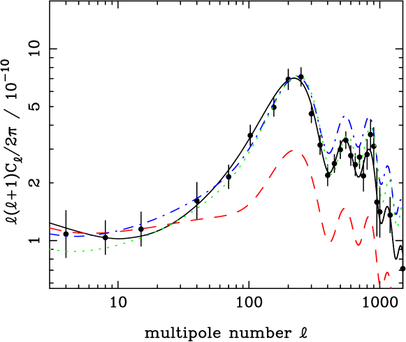
Figure 20: The tensor degeneracy. Adding a large tensor component to an $n=1$ scalar model (solid line) greatly lowers the peak (dashed line), once COBE normalization is imposed. Tilting to $n=1.3$ cures this (dot-dashed line), but the 2nd and subsequent harmonics are too high. Raising the baryon density by a factor 1.5 (dotted line) leaves us approximately back where we started.

8.3 Tensor degeneracy

All of the above applies to models in which scalar modes dominate. The possibility of a large tensor component yields additional degeneracies, as shown in figure 20. An $n=1$ model with a large tensor component can be made to resemble a zero-tensor model with large blue tilt ($n>1$) and high baryon content. Efstathiou et al. (2002) show that adding LSS data does not remove this degeneracy; this is reasonable, since LSS data only constrain the baryon content weakly. A better way of limiting the possible tensor contribution is to look at the amplitude of mass fluctuations today: this normalization of the scalar component is naturally lower if the CMB signal is dominated by tensors. These issues are discussed further below.

Another way in which the remaining degeneracy may be lifted is through polarization of the CMB fluctuations. A nonzero polarization is inevitable because the electrons at last scattering experience an anisotropic radiation field. Thomson scattering from an anisotropic source will yield polarization, and the practical size of the fractional polarization $P$ is of the order of the quadrupole radiation anisotropy at last scattering: $P\mathrel{\lower 2.58334pt\hbox{$\buildrel{\textstyle>}\over{\scriptstyle\sim}$}}1$%. This signal is expected to peak at $\ell\simeq 500$, and the effect was first seen by the DASI experiment (Kovac et al. 2002). Much more detailed polarization results were presented by the WMAP satellite, including a critical detection of large-scale polarization arising from secondary scattering at low $z$, thus measuring the optical depth to last scattering (Kogut et al. 2003). On large scales, the polarization signature of tensor perturbations differs from that of scalar perturbations (e.g. Seljak 1997; Hu & White 1997); the different contributions to the total unpolarized $C_{\ell}$ can in principle be disentangled, allowing the inflationary test to be carried out.

9 Combination of the CMB and large-scale structure

The 2dFGRS power spectrum contains important information about the key parameters of the cosmological model, but we have seen that additional assumptions are needed, in particular the values of $n$ and $h$. Observations of CMB anisotropies can in principle measure most of the cosmological parameters, and combination with the 2dFGRS can lift most of the degeneracies inherent in the CMB-only analysis. It is therefore of interest to see what emerges from a joint analysis.

The clearest immediate result is that the geometrical degeneracy becomes broken (Efstathiou et al. 2002). A 95% confidence upper limit on any curvature can be set at $|\Omega-1|<0.05$. We can therefore be confident that the universe is very nearly flat so it is defensible to assume hereafter that this is exactly true. The importance of tensors will of course be one of the key questions for cosmology over the next several years, but it is interesting to consider the limit in which these are negligible. In this case, the standard model for structure formation contains a vector of only 6 parameters:

$${\bf p}=(n_{s},\Omega_{m},\Omega_{b},h,Q,\tau).$$ (157)

Of these, the optical depth to last scattering, $\tau$, is almost entirely degenerate with the normalization, $Q$ – and indeed with the bias parameter; we discuss this below. The remaining four parameters are pinned down very precisely: using a compilation of pre-WMAP CMB data plus the 2dFRGS power spectrum, Percival et al. (2002) obtained

$$(n_{s},\omega_{c},\omega_{b},h)=(0.963\pm 0.042,0.115\pm 0.009,0.021\pm 0.002,0.665\pm 0.047),$$ (158)

or an overall density parameter of $\Omega_{m}=0.313\pm 0.055$.

It is remarkable how well these figures agree with completely independent determinations: $h=0.72\pm 0.08$ from the HST key project (Mould et al. 2000; Freedman et al. 2001); $\Omega_{b}h^{2}=0.020\pm 0.001$ (Burles et al. 2001). This gives confidence that the tensor component must indeed be sub-dominant.

This analysis was published in Percival et al. (2002), and is based on the preliminary version of the 2dFGRS power spectrum, from Percival et al. (2001). We can make a first estimate of how this is likely to change using the $\Omega_{m}h=0.18\pm 0.02$ from the preliminary analysis of $P(k)$ from the final dataset. In combination with the WMAP $\Omega_{m}h^{3.4}=0.084$ from the CMB peak degeneracy, this yields

$$\Omega_{m}=0.25\pm 15\%\quad h=0.73\pm 5\%$$ (159)

as the preferred current figures from an analysis of this type. The matter density remains frustratingly imprecise, and it is clear that it will be very hard to measure $h$ accurately enough to cure this problem. However, complementary constraints on $\Omega_{m}$ exist at similar precision (e.g. $\Omega_{m}=0.28\pm 18\%$ for a flat model from the SNe Ia Hubble diagram; Tonry et al. 2003). With new results from gravitational lensing, $\Omega_{m}$ should be measured to better than 10% precision within a year.

Perhaps the most striking conclusion from these results concerns the nature of the primordial fluctuations, which remain consistent with the $n=1$ scale-invariant form. The WMAP analysis of Spergel et al. (2003) yields $0.97\pm 0.03$ from CMB plus 2dFGRS (cf. $0.96\pm 0.04$ from Percival et al. 2002). The WMAP team also consider adding data from the Lyman-$\alpha$ forest, which pushes the solution away from a pure power-law:

$$n=0.93\pm 0.03\quad\quad{dn\over d\ln k}=-0.031\pm 0.016.$$ (160)

This evidence for running of $n$ is at best marginal, and disappears completely when systematic uncertainties in the Lyman-$\alpha$ data are considered (Seljak, McDonald & Makarov 2003). It would in any case be surprising if true, since simple inflation models suggest that $dn/d\ln k$ should be second order in $(n-1)$. Although the tensor degeneracy prevents any very strong statements, the data are best described by pure scalar fluctuations, and Percival et al. (2002) set an upper limit of 0.7 to the tensor-to-scalar ratio.

The agreement with pure scalar $n=1$ is not yet a strong embarrassment for inflation, but it is starting to bite on some inflationary models. Leach & Liddle (2003) show that CMB plus 2dFGRS are inconsistent with the $V=\lambda\phi^{4}$ model at just about 95% confidence. It is possible to set up inflation models in which tilt and tensors are both negligible, but there has been a long-standing hope for more substantial signs of inflationary dynamics; if these are not seen soon, it will be a major disappointment.

9.1 Matter fluctuation amplitude and bias

The above conclusions were obtained by considering the shapes of the CMB and galaxy power spectra. However, it is also of great interest to consider the amplitude of mass fluctuations, since a comparison with the galaxy power spectrum allows us to infer the degree of bias directly. This analysis was performed by Lahav et al. (2002). Given assumed values for the cosmological parameters, the present-day linear normalization of the mass spectrum (e.g. $\sigma_{8}$) can be inferred. It is convenient to define a corresponding measure for the galaxies, $\sigma_{8{\rm g}}$, such that we can express the bias parameter as

$$b=\frac{\sigma_{8{\rm g}}}{\sigma_{8{\rm m}}}.$$ (161)

In practice, we define $\sigma_{8{\rm g}}$ to be the value required to fit a CDM model to the power-spectrum data on linear scales ($0.02<k<0.15{\,h\,\rm Mpc^{-1}}$). The amplitude of 2dFGRS galaxies in real space estimated by Lahav et al. (2002) is $\smash{\sigma_{8{\rm g}}^{R}}(L^{*})=0.76$, with a negligibly small random error. This assumes no evolution in $\smash{\sigma_{8{\rm g}}}$, plus the luminosity dependence of clustering measured by Norberg et al. (2001).

The value of $\sigma_{8}$ for the dark matter can be deduced from the CMB fits. Percival et al. (2002) obtain

$$\sigma_{8}\exp(-\tau)=0.72\pm 0.04,$$ (162)

where the error bar includes both data errors and theory uncertainty. The WMAP number here is almost identical: $\sigma_{8}\exp(-\tau)=0.71$, but no error is quoted (Spergel et al. 2003). The unsatisfactory feature is the degeneracy with the optical depth to last scattering. For reionization at redshift $8$, we would have $\tau\simeq 0.05$; it is not expected theoretically that $\tau$ can be hugely larger, and popular models would place reionization between $z=10$ and $z=15$, or $\tau\simeq 0.1$ (e.g. Loeb & Barkana 2001). One of the many impressive aspects of the WMAP results is that they are able to infer $\tau=0.17\pm 0.04$ from large-scale polarization. Taken at face value, $\tau=0.17$ would argue for reionization at $z=20$, but the error means that more conventional figures are far from being ruled out. Taking all this together, it seems reasonable to assume that the true value of $\sigma_{8}$ is within a few % of 0.80. Given the 2dFGRS figure of $\smash{\sigma_{8{\rm g}}^{R}}=0.76$, this implies that $L^{*}$ galaxies are very nearly exactly unbiased. Since there are substantial variations in the clustering amplitude with galaxy type, this outcome must be something of a coincidence. This conclusion of near-unity bias was reinforced in a completely independent way, by using the measurements of the bispectrum of galaxies in the 2dFGRS (Verde et al. 2002). As it is based on three-point correlations, this statistic is sensitive to the filamentary nature of the galaxy distribution – which is a signature of nonlinear evolution. One can therefore split the degeneracy between the amplitude of dark-matter fluctuations and the amount of bias.

These conclusions point the way towards a possible limit on the tensor contribution: a large contribution of tensors to the COBE signal would lower the required scalar amplitude. As an extreme example, a scalar-to-tensor ratio of 1 would reduce the ‘apparent’ $\sigma_{8}$ by roughly a factor of $\sqrt{2}$, to 0.5. Even for an implausibly large value of $\tau$, this would be hard to reconcile with the level of galaxy clustering plus the requirement of a low degree of bias. Also, more direct limits on $\sigma_{8}$ are now being derived from large-scale gravitational lensing surveys, with $\sigma_{8}\simeq 0.7$ to 0.8 being favoured (e.g. Brown et al. 2003; Jarvis et al. 2003).

10 Less-standard ingredients

10.1 Limits to the neutrino mass

Even though a CDM-dominated universe matches the data very well, there are many plausible variations to consider. Probably the most interesting is the neutrino mass: experimental data on neutrino oscillations mean that at least one neutrino must have a mass of $\mathrel{\lower 2.58334pt\hbox{$\buildrel{\textstyle>}\over{\scriptstyle\sim}$}}0.05$ eV, so that $\Omega_{\nu}\mathrel{\lower 2.58334pt\hbox{$\buildrel{\textstyle>}\over{\scriptstyle\sim}$}}10^{-3}$ – the same order of magnitude as stellar mass.

Figure 21: Results from Elgaroy et al. (2002), who considered constraints on the neutrino mass from 2dFGRS. The first panel shows Power spectra for $\Omega_{\nu}=0$ (solid line), $\Omega_{\nu}=0.01$ (dashed line), and $\Omega_{\nu}=0.05$ (dot-dashed line) with amplitudes fitted to the 2dFGRS power spectrum data (vertical bars). Other parameters are fixed at $\Omega_{\rm m}=0.3$, $\Omega_{\Lambda}=0.7$, $h=0.7$, $\Omega_{\rm b}h^{2}=0.02$. The vertical dashed lines limit the range in $k$ used in the fits. The second panel shows 68% (solid line), 95% (dashed line) and 99% (dotted line) confidence contours in the plane of $f_{\nu}\equiv\Omega_{\nu}/\Omega_{\rm m}$ and $\Gamma\equiv\Omega_{\rm m}h$, with marginalization over $h$ and $\Omega_{\rm b}h^{2}$ using Gaussian priors.

As explained in earlier, a non-zero neutrino mass can lead to relatively enhanced large-scale power, beyond the neutrino free-streaming scale. This is illustrated in figure 21, taken from Elgaroy et al. (2002). Broadly speaking, allowing a significant neutrino mass changes the spectrum in a way that resembles lower density, so there is a near-degeneracy between neutrino mass fraction and $\Omega_{m}h$ (figure 21). A limit on the neutrino fraction thus requires a prior on $\Omega_{m}h$. Based on the cluster baryon fraction plus BBN, Elgaroy et al. adopt $\Omega_{m}<0.5$; together with the HST Hubble constant, this yields a marginalized 95% limit of $f_{\nu}<0.13$, or $m_{\nu}<1.8$ eV. Note that this is the sum of the eigenvalues of the mass matrix: given neutrino oscillation results (e.g. Ahmad et al. 2002; Eguchi et al. 2003), the only way a cosmologically significant density can arise is via a nearly degenerate hierarchy, so this allows us to deduce $m_{\nu}<0.6$ eV for any one species. Including the latest WMAP results in order to set a more strict limit on $\Omega_{m}h$, this limit falls to 0.23 eV (Spergel et al. 2003).

10.2 The equation of state of the vacuum

So far, we have assumed that the vacuum energy is exactly a classical $\Lambda$, or at any rate indistinguishable from one. This is a highly reasonable prior: there is no reason for the asymptotic value of any potential to go exactly to zero, so one always needs to solve the classical cosmological constant problem – for which probably the only reasonable explanation is an anthropic one (e.g. Vilenkin 2001). Therefore, dynamical provision of $w\equiv p_{v}/\rho_{v}\neq-1$ is not needed. Nevertheless, one can readily take an empirical approach to $w$ (treated as a constant for a first approach).

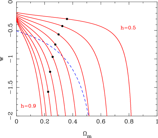
Figure 22: The $\Omega_{m}h^{3.4}$ degeneracy for flat models gives an almost exact value of $\Omega_{m}$ from the CMB is $h$ is known, assuming the vacuum to be effectively a classical $\Lambda$ ($w=-1$). If $w$ is allowed to vary, this becomes a locus on the $(\Omega_{m},w)$ plane (similar to the locus for best-fitting flat models from the SNe, showed dotted). Solid circles show values of $\Omega_{m}h$ that satisfy the updated 2dFGRS constraint of 0.18 (suppressing error bars).

Figure 22 shows a simplified approach to this, plotting the locus on $(w,\Omega_{m})$ space that is required for a given value of $h$ if the location of the main CMB acoustic peak is known exactly. For $h\simeq 0.7$, this is very similar to the locus derived from the SN Hubble diagram (Garnavich et al. 1998). The solid circles show the updated 2dFGRS constraint of $\Omega_{m}h=0.18$. In order to match the data with $w$ closer to zero, $\Omega_{m}$ must increase and $h$ must decrease. The latter trend means that the HST Hubble constant sets an upper limit to $w$ of about $-0.54$ (Percival et al. 2002). This is very similar to the SNe constraint of Garnavich et al. (1998), so the combined limit is already close to $w<-0.8$. The vacuum energy is indeed looking rather similar to $\Lambda$.

10.3 The total relativistic density

Finally, an interesting aspect of figure 22 is that it reminds us of history. When the COBE detection was announced in 1992, a popular model was ‘standard’ CDM with $\Omega_{m}=1$, $h=0.5$. As we see, this comes close to fitting the CMB data, and such a model is not unattractive in some ways. Can we be sure it is ruled out? Leaving aside the SNe data, one might think to evade the 2dFGRS constraint by altering the total relativistic content of the universe (for example, by the decay of a heavy neutrino after nucleosynthesis). Since 2dFGRS measures the horizon at matter-radiation equality, this will be changed. If the radiation density is arbitrarily boosted by a factor $X$, the constraint from LSS becomes

$$(\Omega_{m}h)_{\rm apparent}=X^{-1/2}(\Omega_{m}h)_{\rm true}.$$ (163)

Therefore $X\simeq 8$ is required to allow an Einstein–de Sitter universe.

However, this argument fails, because it does not take into account the effect of the extra radiation on the CMB. As argued above, the location of the acoustic peaks depends on $a_{\rm eq}$, which depends on $\omega_{m}$. However, if we change the radiation content, then what matters is $\omega_{m}/X$. Thus, the CMB peak constraint now reads

$$\Omega_{m}^{-0.1}(\omega_{m}/X)^{0.24}={\rm constant};$$ (164)

when combining LSS and CMB, everything is as before except that the effective Hubble parameter is $h/X^{1/2}$. Thus, a model with $\Omega_{m}=1$ but boosted radiation would only fit the CMB with $h\simeq 0.5\sqrt{8}\simeq 1.4$, and the attractiveness of a low age is lost. In any case, combining LSS and CMB would give the same $\Omega_{m}\simeq 0.3$ independent of $X$, so it is impossible to save models with $\Omega_{m}=1$ by this route.

Finally, it is interesting to invert this argument. Since Percival et al. (2002) obtain an effective $h$ of $0.665\pm 0.047$ and Freedman et al. (2001) measure $h=0.72\pm 0.08$, we deduce

$$1.68X=1.82\pm 0.24.$$ (165)

This convincingly rules out the $1.68X=1$ that would apply if the universe contained only photons, and amounts to a detection of the neutrino background. In terms of the number of neutrino species, this is $N_{\nu}=3.6\pm 1.1$. A more precise result is of course obtained from primordial nucleosynthesis, but this applies at a much later epoch, thus constraining models with decaying particles.

11 Conclusions

The beautiful data on the large-scale structure of the universe revealed in particular by the 2dF Galaxy Redshift Survey combine with the incredible recent progress in CMB data to show spectacularly good agreement with a ‘standard model’ for structure formation. This consists of a scalar-mode adiabatic CDM universe with scale-invariant fluctuations. Measuring the exact parameters of this model is rendered difficult by the intrinsic degeneracies of the structure-formation process, but progress is being made. The most recent data yield $\Omega_{m}=0.25\pm 15\%$ and $h=0.73\pm 5\%$; these figures accord well with independent constraints, and it is very hard to believe that they are incorrect.

Allowing extra degrees of freedom, such as massive neutrinos, vacuum equation of state $w\neq 1$, or extra relativistic content worsens the agreement with independent constraints on $h$ and $\Omega_{m}$. This both supports the simplest picture and allows us to set interesting limits on these non-standard ingredients.

For the future, we can look with anticipation to meaningful tests of inflation: the current data are consistent with $n=1$ to an error of $\pm 0.03$, and the errors may be expected to halve over the next couple of years, bringing plausible levels of tilt well within the reach of experimental detection. A demonstration that $n\neq 1$ would be a large step in the direction of proving inflation to be true, so the cosmological stakes over the next few years will be high. The tensor fraction is a less clear target, but the motivation to improve on the current weak upper limits will remain strong.

It should of course not be forgotten that the large-scale structure we measure locally consists of galaxies. In these lectures, the physics of galaxy formation has been largely ignored, but this will be the increasing focus of LSS studies: not just the global parameters of the universe, but the detailed understanding of how the complex structures around us formed.

References

Adelberger K. et al., 1998, ApJ, 505, 18

Adler R.J., 1981, The Geometry of Random Fields, Wiley

Ahmad Q.R. et al. (the SNO Consortium), 2002, Phys. Rev. Lett., 89, 011301

Bardeen J.M., 1980, Phys. Rev. D, 22, 1882

Bardeen J.M., Bond J.R., Kaiser N., Szalay A.S., 1986, Astrophys. J., 304, 15

Baugh C.M., Efstathiou G., 1993, MNRAS, 265, 145

Baugh C.M., Efstathiou G., 1994, MNRAS, 267, 323

Bahcall N.A., Soneira R.M., 1983, ApJ, 270, 20

Benoist C., Maurogordato S., da Costa L.N., Cappi A., Schaeffer R., 1996, ApJ, 472, 452

Benson A.J., Cole S., Frenk C.S., Baugh C.M., Lacey C.G., 2000a, Mon. Not. R. Astr. Soc., 311, 793

Benson A.J., Baugh C.M., Cole S., Frenk C.S., Lacey C.G., 2000b, Mon. Not. R. Astr. Soc., 316, 107

Benson, A.J., Frenk, C.S., Baugh, C.M., Cole, S., Lacey, C.G., 2001, MNRAS, 327, 1041

Bond J.R., Cole S., Efstathiou G., Kaiser N., 1991, Astrophys. J., 379, 440

Bond J.R., Efstathiou G., 1984, Astrophys. J., 285, L45

Bond J.R., Szalay A., 1983, ApJ, 274, 443

Bouchet F.R., Colombi S., Hivon E., Juszkiewicz R., 1995, Astr. Astrophys., 296, 575

Brown M.L. et al., 2003, MNRAS, 341, 100

Bucher M., Moodley K., Turok, N., 2002, Phys. Rev. D, 66, 023528

Burles S., Nollett K.M., Turner M.S., 2001, ApJ, 552, L1

Carlberg R.G., Couchman H.M.P., Thomas P.A., 1990, Astrophys. J., 352, L29

Carroll S.M., Press W.H., Turner E.L., Ann. Rev. Astr. Astrophys., 30, 499

Colberg J. et al., 2000, MNRAS, 319, 209

Cole S., Aragón-Salamanca A., Frenk C.S., Navarro J.F., Zepf S.E., 1994, Mon. Not. R. Astr. Soc., 271, 781

Cole S., Hatton S., Weinberg D.H., Frenk C.S., 1998, MNRAS, 300, 945

Cole S., Lacey C.G., Baugh C.M., Frenk C.S., 2000, Mon. Not. R. Astr. Soc., 319, 168

Cole S., Kaiser N., 1989, Mon. Not. R. Astr. Soc., 237, 1127

Coles P., 1993, Mon. Not. R. Astr. Soc., 262 ,1065

Coles P., Jones B.J.T., 1991, Mon. Not. R. Astr. Soc., 248, 1

Colless M. et al., 2001, MNRAS, 328, 1039

Croft R.A.C., Dalton G.B., Efstathiou G., Sutherland W.J., Maddox S.J., 1997, MNRAS, 291, 305

Davis M., Peebles P.J.E., 1983, ApJ, 267, 465

Davis M., Geller M.J., 1976, ApJ, 208, 13

Davis M., Efstathiou G., Frenk C.S., White S.D.M., 1985, Astrophys. J., 292, 371

Dekel A., Rees M.J., 1987, Nat, 326, 455

Dekel A., Lahav O., 1999, ApJ, 520, 24

de Lapparant V., Geller M.J., Huchra J.P., 1986, ApJ, 302, L1

Dodelson S., 2003, Modern Cosmology, Academic Press

Efstathiou G. et al., 2002, MNRAS, 330, L29

Efstathiou G., Bond J.R., 1986, MNRAS, 218, 103

Efstathiou G., Bond J.R., 1999, MNRAS, 304, 75

Efstathiou G., Davis M., White S.D.M., Frenk C.S., 1985, Astrophys. J. Suppl., 57, 241

Eguchi K. et al., 2003, Phys. Rev. Lett., 90, 1802

Eisenstein D.J., Hu W., 1998, ApJ, 496, 605

Eisenstein D.J., Hu W., 1999, ApJ, 511, 5

Eke V.R., Cole S., Frenk C.S., 1996, Mon. Not. R. Astr. Soc., 282, 263

Elgaroy O. et al., 2002, Phys. Rev. Lett., 89, 061301

Evrard A. et al., 2002, ApJ, 573, 7

Evrard A., 1997, MNRAS, 292, 289

Feldman H.A., Kaiser N., Peacock J.A., 1994, ApJ, 426, 23

Freedman W.L. et al., 2001, ApJ, 553, 47

Fry J.N., 1986, ApJ, 461, L65

Garnavich P.M. et al., 1998, ApJ, 509, 74

Ghigna S., Moore B., Governato F., Lake G., Quinn T., Stadel J., 1998, Mon. Not. R. Astr. Soc., 300, 146

Goldberg D.M., Strauss M., 1998, ApJ, 495, 29

Gordon C., Lewis A., 2002, astro-ph/0212248

Hambly N.C., Irwin M.J., MacGillivray H.T., 2001, MNRAS, 326 1295

Hawking S., 1982, Phys. Lett., B115, 29

Hawkins E. et al., 2002, astro-ph/0212375

Heath D., 1977, Mon. Not. R. Astr. Soc., 179, 351

Hernquist L., Bouchet F.R., Suto Y., 1991, Astrophys. J. Suppl., 75, 231

Hockney R. W., Eastwood J. W., 1988, Computer Simulations Using Particles, IOP Publishing

Hu W., Dodelson S., 2002, ARAA, 40, 171

Hu W., Fukugita M., Zaldarriaga M., Tegmark M., 2001, ApJ, 549, 669

Hu W., Sugiyama N., 1995, ApJ, 444, 489

Hu W., White M., 1997, New Astronomy, 2, 323

Hubble E.P., 1934, ApJ, 79, 8

Jarvis M. et al., 2003, AJ, 125, 1014

Jenkins A., Frenk C.S., Pearce F.R., Thomas P.A., Colberg J.M., White S.D.M., Couchman H.M.P., Peacock J.A., Efstathiou G., Nelson A.H., 1998, ApJ, 499, 20

Jing Y.P., Mo H.J., Börner G., 1998, ApJ, 494, 1

Kaiser N., 1984, ApJ, 284, L9

Katz N., Weinberg D.H., Hernquist L., 1996, ApJ Suppl., 105, 19

Kauffmann G., Colberg J.M., Diaferio A., White S.D.M., 1999, Mon. Not. R. Astr. Soc., 303, 188

Kauffmann G., Nusser A., Steinmetz M., 1997, Mon. Not. R. Astr. Soc., 286, 795

Kauffmann G., White S.D.M., Guiderdoni B., 1993, Mon. Not. R. Astr. Soc., 264, 201

Kirshner R.P., Oemler A., Schechter P.L., Shectman S.A., 1981, Astrophys. J., 248, L57

Klypin A., Kopylov A.I., 1983, Soviet Astron. Lett., 9, 41

Klypin A., Primack J., Holtzman J., 1996, Astrophys. J., 466, 13

Klypin A., Gottlöber S., Kravtsov A.V., Khokhlov A.M., 1999, ApJ, 516, 530

Kodama H., Sasaki M., 1984, Prog. Theor. Phys. Suppl., 78, 1

Kovac J.M. et al., 2002, Nature, 420, 772

Kogut A. et al., 2003, astro-ph/0302213

Kravtsov A.V., Klypin A.A., Khokhlov A.M., 1997, ApJ Suppl., 111, 73

Kuo C.L. et al., 2002, astro-ph/0212289

Lahav O., Lilje P.B., Primack J.R., Rees M.J., 1991, Mon. Not. R. Astr. Soc., 251, 128

Lahav O. et al., 2002, MNRAS, 333, 961

Leach S.M., Liddle A.R., 2003, astro-ph/0306305

Lewis I.J. et al., 2002, MNRAS, 333, 279

Liddle A.R., Lyth D., 2000, Cosmological inflation & large-scale structure, CUP

Loeb A., Barkana R., 2001, ARAA, 39, 19

Loveday J., Maddox S.J., Efstathiou G., Peterson B.A., 1995, Astrophys. J., 442, 457

Lyth D., Wands D., 2002, Phys. Lett., B524, 5

Ma C.-P., 1999, Astrophys. J., 510, 32

Ma C.-P., 1996, Astrophys. J., 471, 13

Maddox S.J., Efstathiou G., Sutherland W.J., Loveday J., 1990a, MNRAS, 242, 43p

Maddox S.J., Sutherland W.J., Efstathiou G., Loveday J., 1990b, MNRAS, 243, 692

Maddox S.J., Efstathiou G., Sutherland W.J., 1990c, MNRAS, 246, 433

Mann R.G., Peacock J.A., Heavens A.F., 1998, MNRAS, 293, 209

Meiksin A.A., White M., Peacock J.A., 1999, MNRAS, 304, 851

Mészáros P., 1974, Astr. Astrophys., 37, 225

Mo H.J., White S.D.M., 1996, MNRAS, 282, 1096

Moore B., Frenk C.S., White S.D.M., 1993, Mon. Not. R. Astr. Soc., 261, 827

Moore B., Quinn T., Governato F., Stadel J., Lake G., 1999, Mon. Not. R. Astr. Soc., 310, 1147 [M99]

Mould J.R. et al., 2000, ApJ, 529, 786

Mukhanov V.F., Feldman H.A., Brandenberger R.H., 1992, Phys. Reports, 215, 203

Narayanan V.K., Spergel D.N., Davé R., Ma C.-P., 2000, ApJ, 543, L103

Navarro J.F., Frenk C.S., White S.D.M., 1996, ApJ, 462, 563

Neyman J., Scott E.L. & Shane C.D., 1953, ApJ, 117, 92

Norberg P. et al., 2001, MNRAS, 328, 64

Nusser A., 2000, MNRAS, 317, 902

Papovich C., Dickinson M., Ferguson H.C., 2001, ApJ, 559, 620

Peacock J.A., 1997, Mon. Not. R. Astr. Soc., 284, 885

Peacock J.A., 1999, Cosmological Physics, CUP

Peacock J.A., Smith R.E., 2000, Mon. Not. R. Astr. Soc., 318, 1144

Pearce F.R. et al., 1999, Astrophys. J., 521, L99

Pearce F.R. et al., 2001, MNRAS, 326, 649

Pearson T.J. et al., 2002, astro-ph/0205388

Peebles P.J.E., 1974, A&A, 32, 197

Peebles P.J.E., 1980, The Large-Scale Structure of the Universe, Princeton Univ. Press, Princeton, NJ

Peebles P.J.E., Yu J.T., 1970, Astrophys. J., 162, 815

Peebles P.J.E., 1987, Nature, 327, 210

Pen U.-L., 1998, ApJ, 504, 601

Percival W.J. et al., 2001, MNRAS, 327, 1297

Percival W.J. et al., 2002, MNRAS, 337, 1068

Pogosyan D., Starobinsky A.A., 1995, Astrophys. J., 447, 465

Press W.H., Schechter P., 1974, Astrophys. J., 187, 425

Press W.H., Teukolsky S.A., Vetterling W.T., Flannery B.P., Numerical Recipes (2nd edition), Cambridge University Press

Rees M.J., 1985, Mon. Not. R. Astr. Soc., 213, 75

Saunders W., Frenk C., Rowan-Robinson M., Efstathiou G., Lawrence A., Kaiser N., Ellis R., Crawford J., Xia X.-Y., Parry I., 1991, Nature, 349, 32

Schlegel D.J., Finkbeiner D.P., Davis M., 1998, ApJ, 500, 525

Seljak U., 1997, Astrophys. J., 482, 6

Seljak U., 2000, MNRAS, 318, 203

Seljak U., Zaldarriaga M., 1996, Astrophys. J., 469, 437

Seljak U., McDonald P. Makarov A., 2003, astro-ph/0302571

Sheth R.K., Tormen G., 1999, Mon. Not. R. Astr. Soc., 308, 119

Sheth R.K., Mo H.J., Tormen G., 2001, MNRAS, 323, 1

Smoot G.F. et al., 1992, Astrophys. J., 396, L1

Somerville R.S., Primack J.R., 1999, Mon. Not. R. Astr. Soc., 310, 1087

Spergel D.N. et al., 2003, astro-ph/0302209

Starobinsky A.A., 1985, Sov. Astr. Lett., 11, 133

Stoughton C.L. et al., 2002, AJ, 123, 485

Sugiyama N., 1995, Astrophys. J. Suppl., 100, 281

Tegmark M., Peebles P.J.E., 1998, ApJ, 500, L79

Tonry J.L. et al., 2003, astro-ph/0305008

Valageas P., 1999, A&A, 347, 757

van Kampen E., 2000, astro-ph/0002027

van Kampen E., Jimenez R., Peacock J.A., 1999, Mon. Not. R. Astr. Soc., 310, 43

Verde L. et al., 2002, MNRAS, 335, 432

Vilenkin A., 2001, hep-th/0106083

Vittorio N., Silk J., 1985, ApJ, 297, L1

White S.D.M., Rees M., 1978, Mon. Not. R. Astr. Soc., 183, 341

White S.D.M., Davis M., Efstathiou G., Frenk C.S., 1987, Nature, 330, 451

Zehavi I. et al., 2003, astro-ph/0301280

Zeldovich Y.B., 1970, Astr. Astrophys., 5, 84

Zwicky F., 1933, Helv. Phys. Acta, 6, 110