Thermo-Hydrodynamics of Circumstellar Disks
with High-mass Planets

Abstract

With a series of numerical simulations, we analyze the thermo-hydrodynamical evolution of circumstellar disks containing Jupiter-size protoplanets. In the framework of the two-dimensional approximation, we consider an energy equation that includes viscous heating and radiative effects in a simplified, yet consistent form. Multiple nested grids are used in order to study both global and local features around the planet. By means of different viscosity prescriptions, we investigate various temperature regimes. A planetary mass range from $0.1$ to $1\;\mbox{$M_{\mathrm{J}}$}$ is examined. Computations show that gap formation is a general property which affects density, pressure, temperature, optical thickness, and radiated flux distributions. However, it remains a prominent feature only when the kinematic viscosity is on the order of $10^{15}\;\mbox{$\mathrm{cm}^{\mathrm{2}}\,\mathrm{s}^{\mathrm{-1}}$}$ or lower, though it becomes rather shallow for $0.1\,\mbox{$M_{\mathrm{J}}$}$ perturbers. Around accreting planets, a circumplanetary disk forms that has a surface density profile decaying exponentially with the distance and whose mass is $5$–$6$ orders of magnitudes smaller than Jupiter’s mass. Circumplanetary disk temperature profiles decline roughly as the inverse of the distance from the planet, matching the values measured in the gap toward the border of the Roche lobe. Temperatures range from some $10$ to $\sim 1000\;\mbox{$\mathrm{K}$}$. Moreover, circumplanetary disks are generally opaque, with optical thickness larger than $1$ and aspect ratios around a few tenths. Non-accreting protoplanets provide quite different scenarios, with a clockwise, i.e., reversed flow rotation around low-mass bodies. Planetary accretion and migration rates depend on the viscosity regime, with discrepancies within an order of magnitude. Coorbital torques increase as viscosity increases. For high viscosities, Type I migration may extend to larger planetary masses. Estimates of growth and migration time scales inferred by these models are on the same orders of magnitude as those previously obtained with locally isothermal simulations, both in two and three dimensions.

1 Introduction

Since the very first attempt of modeling a protoplanet interacting with its primitive nebula by Miki (1982), two decades have passed. Seventeen years had to go by for tackling this problem with the strength of new and more powerful computational tools (Bryden et al., 1999; Kley, 1999; Lubow, Seibert, & Artymowicz, 1999; Miyoshi et al., 1999). As a consequence of the mounting interest in extrasolar planets, boosted by eight years of uninterrupted new detections, the scientific community has made an extraordinary effort, over the past four years, to analyze disk-planet interactions by means of numerical calculations.

Yet, regardless of the processes accounted for in the implemented numerical models, limitations and restrictions remain an issue to deal with. As a matter of fact, numerical calculations still lag behind the present knowledge of the possible physical effects which occur in a circumstellar environment containing massive bodies. Thereupon, simplifying assumptions are always demanded. Nonetheless, steps forward have been made in many directions to reduce their number.

Three-dimensional (3D) disks containing Jupiter-size objects have been investigated by Kley, D’Angelo, & Henning (2001) and, including also magnetic fields, by Papaloizou & Nelson (2003), Nelson & Papaloizou (2003), and Winters, Balbus, & Hawley (2003). D’Angelo, Henning, & Kley (2002, hereafter Paper I) carried out global two-dimensional (2D) high-resolution simulations of Jupiter-mass as well as Earth-mass planets, resolving also the flow structure within the planetary’s Roche lobe by applying a resolution enhancement strategy. This study has been lately extended to the 3D space by D’Angelo, Kley, & Henning (2003, hereafter Paper II) and by Bate et al. (2003), who used instead a single grid with variable step size. Nelson & Benz (2003a, b) performed 2D computations, considering the effects due to disk self-gravity. Morohoshi & Tanaka (2003) have investigated the interactions between a planet and an optically thin disk with local simulations in the shearing sheet approximation, in order to determine the one-sided gravitational torque acting on the planet.

With the present work we intend to relax the widely adopted local-isothermal approximation, i.e., that of treating a disk as a system having a fixed temperature distribution which depends neither on time nor on any other system variable. Yet, we will preserve the global viewpoint which we believe to be crucial because disk-planet interactions can be highly non-local.

Many of the sophisticated accretion disk studies adopt 2D or 1+1D schemes due to the difficulty of dealing with all the necessary ingredients in a full 3D space. Until very recently, in fact, radiation (e.g., Dullemond et al., 2002), convection (e.g., Agol et al., 2001), magnetic fields (e.g., Matt et al., 2002) , mixtures of gas and dust (e.g., Suttner & Yorke, 2001), and chemical evolution (e.g., Markwick et al., 2002) have been treated via two-dimensional models. Furthermore, numerical simulations generally involve parameter studies, because many physical quantities are poorly known. Thereby, with a restricted number of dimensions, one is at least able to acquire a spectrum of possible approximate solutions.

In order to overcome the local-isothermal hypothesis and to maintain a global approach at the same time, we introduce an energy transport in 2D ($r$–$\varphi$) models. We include all the supposedly major causes responsible for generation, transfer, and loss of energy in low-temperature circumstellar disk environments. We take advantage of the small aspect ratio of the disk, and assume that all the radiation transport is effective only in the vertical direction. Such approximation works reasonably well in accretion disks, away from the boundary and surface layers (see, e.g., Pringle, 1981). Though such an approach relies on the “slimness” assumption, it is as well appropriate in the local environment around a protoplanet. In fact, around there, the disk becomes even thinner when the planet’s gravitational action is accounted for. Hence, the amount of energy transported by radiation in the vertical direction still overwhelms that transported horizontally. Although this represents a simplistic kind of thermal description, it allows to investigate processes which have not been considered thus far, i.e., the joint thermo-hydrodynamical evolution of disk-planet interactions. Furthermore, since these simulations benefit of a nested-grid numerical technique (Paper I, Paper II), though relying on the global approach we are capable of achieving resolutions large enough to accurately describe the system within the planetary’s Roche lobe.

The outline of the paper is the following. In the next section we introduce the physical formulation of the problem, focusing on the equation for the thermal energy density and related issues. Section 3 concerns the numerical method utilized to solve the energy equation along with a series of tests. In § 4 we specify the adopted parameters and other various details. Sections 5 and 6 describe, respectively, global and local properties of models with different masses and viscosity regimes. In § 7 we report the results for mass accretion and orbital migration. Our conclusions are presented in § 8.

2 Physical Formalism

As mentioned before, we are going to tackle the problem of energy transfer in an accretion disk with an embedded planet. Since solving the full set of equations in three dimensions and simultaneously achieving sufficient resolution around the protoplanet is computationally difficult at the moment, we restrict to two-dimensional disk models.

The reason for this choice is two-folded. On the one hand, with affordable computational times and sufficiently high resolutions, it allows to investigate the coupling between hydrodynamics and thermodynamics both in the disk and nearby the embedded body. On the other, it permits to adopt a strategic assumption in writing the energy equation, i.e., that the horizontal energy transport can be neglected compared to the vertical one. In other words, in a 2D disk one can assume that radiation transport is only effective along the direction perpendicular to the equatorial plane of the system.

Hence, let us describe the disk material through the Navier-Stokes equations for the surface density $\Sigma$, the linear momentum (density) $\Sigma\,u_{r}$, and the angular momentum (density) $r\,\Sigma\,u_{\varphi}$, where we choose as working coordinate frame a cylindrical one $\{O;r,\varphi,z\}$. The origin is located at the center of mass of the star and the planet while the disk lies in the plane $z=0$. The hydrodynamics equations have been already stated, by using the same notations, in Paper I.

As in most of the computations performed so far, we avoid dealing with the Poisson equation and rather assume that the gravitational field is determined only by the star and the planet, neglecting the self-gravity of the disk material. This is allowed by the circumstance that the Toomre $Q$-parameter is well beyond $1$ in all of our models. Nelson & Benz (2003a, b) found that some effects indeed arise when disk self-gravity is taken into account. However, we note that they consider disk masses ten times as large as those considered here.

Thereby, we rely on a smoothed point-mass gravitational potential, which well reproduces more realistic protoplanetary gravitational potentials (Paper II),

$$\Phi=-\frac{G\,\mbox{$M_{*}$}}{|\boldsymbol{r}-\boldsymbol{r}_{*}|}-\frac{G\,\mbox{$M_{\mathrm{p}}$}}{\sqrt{|\boldsymbol{r}-\boldsymbol{r}_{\mathrm{p}}|^{2}+\delta^{2}}},$$ (1)

where $\boldsymbol{r}_{*}$ and $\boldsymbol{r}_{\mathrm{p}}$ are the radius vectors indicating the positions of the star and the planet, respectively. As done in Paper II, we set the parameter $\delta$ as a constant length (see § 4 for details).

The thermal structure of the fluid has been usually fixed through a power law of the distance $r$. Thereupon, the set of equations has been closed by adding an equation of state which connects the local gas (two-dimensional) pressure to the surface density by means of a local isothermal sound speed $c_{s}^{\mathrm{iso}}$

$$c_{s}^{\mathrm{iso}}=h\,\sqrt{\frac{G\,\mbox{$M_{*}$}}{r}}.$$ (2)

Thus, the Mach number of the flow is considered constant throughout the system’s evolution, constrained solely by the disk aspect ratio $h=H/r$ (e.g., Lubow, Seibert, & Artymowicz, 1999; Miyoshi et al., 1999; Nelson et al., 2000; Tanaka, Takeuchi, & Ward, 2002; Masset, 2002; Nelson & Papaloizou, 2003; Bate et al., 2003; Nelson & Benz, 2003b). Alternatively, Kley (1999) and Tanigawa & Watanabe (2002) did some simulations using a polytropic equation of state of the type $P=\bar{K}\,\Sigma^{\gamma}$. However, the evolution of the thermal properties of the system have not been generally considered.

In the present calculations we use an ideal equation of state which directly ties the gas pressure $P$ to the thermal energy density (energy per unit area) $E$

$$P=(\gamma-1)\,E,$$ (3)

where the adiabatic index $\gamma$ is a constant. Furthermore, if we suppose that disk material behaves as a perfect gas, then the temperature is

$$T=\left(\frac{\mu\,m_{\mathrm{H}}}{k}\right)\frac{P}{\Sigma},$$ (4)

where $\mu$ is the mean molecular weight, $m_{\mathrm{H}}$ is the hydrogen mass, and $k$ the Boltzmann constant. The adiabatic sound speed is given by

$$c_{s}=\sqrt{\gamma\,\left(\frac{k\,T}{\mu\,m_{\mathrm{H}}}\right)}.$$ (5)

Equation (3) implicitly assumes that radiation pressure $P_{\mathrm{rad}}$ is negligibly small compared to gas pressure. Such hypothesis is connected to the relatively low temperature regimes we deal with (in fact $P_{\mathrm{rad}}\propto T^{4}$) and its validity was checked afterward. In all of the models presented here, the ratio $P_{\mathrm{rad}}/P_{\mathrm{gas}}$ never exceeds $10^{-4}$.

2.1 Energy Equation

Equations for energy transport differ according to the processes that have to be included for a correct description of the energy budget of fluid elements. In our case, we suppose that a parcel of disk fluid can gain or lose thermal energy only because of flow advection, compressional work, viscous dissipation, and dissipative effects due to radiation transport. In this sense, rather than strictly treating the transfer of radiation in the disk, we will account only for the cooling effects that radiation causes. Then, the energy equation takes the following form

$$\frac{\partial E}{\partial t}+\nabla\cdot(E\,\boldsymbol{u})=-P\,\nabla\cdot\boldsymbol{u}+\Upsilon-\Lambda.$$ (6)

In equation (6) we indicated with $\Upsilon$ the dissipation function and with $\Lambda$ the radiated energy. In two dimensions, either of these quantities is an energy flux. Both functions are always positive, thereby the former acts as a heating source, whereas the latter as a cooling term. In this study we do not consider convection because we do not expect it to be a major energy source (D’Alessio et al., 1998). Furthermore, we neglect irradiation from the central star which is presumably an effective heating mechanism only in the upper layers of circumstellar disks (see, e.g., D’Alessio et al., 1998), whose effects however are reduced by small disk scale heights. More importantly, as a consequence of the gap formation and the protoplanet’s gravity, circumplanetary material is shielded from stellar radiation, as it will be clarified later.

The function $\Upsilon$ can be directly computed from the components of the viscous stress tensor $S_{rr}$, $S_{\varphi\varphi}$, and $S_{r\varphi}$ (Mihalas & Weibel Mihalas, 1999; Collins, Helfer, & van Horn, 1998)

$$\Upsilon=\frac{1}{2\,\nu\,\Sigma}\left(S^{2}_{rr}+S^{2}_{\varphi\varphi}+S^{2}_{r\varphi}\right)+\frac{2\,\nu\,\Sigma}{9}\,(\nabla\cdot\boldsymbol{u})^{2}.$$ (7)

The divergence term $\nabla\cdot\boldsymbol{u}$ in the equation arises because a three-dimensional definition of stress tensor S is adopted. In fact, the reduction from three to two dimensions is merely achieved by setting the vertical component of the flow field $u_{z}$ and the derivative operator $\partial/\partial z$ to zero.

In a three-dimensional disk, the last term on the right-hand side of equation (6) is equal to $\nabla\cdot\boldsymbol{F}$, where $\boldsymbol{F}$ is the frequency-integrated radiation flux

$$\boldsymbol{F}=-\frac{16\,\sigma_{\mathrm{R}}}{3\,\kappa\,\rho}\,T^{3}\,\nabla T.$$ (8)

In the above equation $\sigma_{\mathrm{R}}$ is the Stefan-Boltzmann constant, $\kappa$ is a frequency-integrated opacity coefficient and $\rho$ is the mass density. As mentioned before, we suppose that the amount of energy transported by radiation in the vertical direction is much larger than that transported horizontally, i.e., $|F_{r}|$ and $|F_{\varphi}|\ll|F_{z}|$. The validity of this statement holds as long as the vertical extent of the disk remains very small compared to the disk characteristic size in the other directions. Thus, in a two-dimensional cylindrical disk we have

$$\Lambda=\int_{-\infty}^{+\infty}\nabla\cdot\boldsymbol{F}\,\mathrm{d}z\simeq\int_{-\infty}^{+\infty}\frac{\partial F_{z}}{\partial z}\,\mathrm{d}z.$$ (9)

Since the vertical disk structure is not meant to be accounted for, it is possible to equate the pressure scale height to the photospheric scale height and assume that all the radiation is liberated at $z=\pm H$. Thereupon, equation (9) becomes

$$\Lambda=\int_{-H}^{+H}\frac{\partial F_{z}}{\partial z}\,\mathrm{d}z=F(H)-F(-H)=2\,F(H).$$ (10)

In 2D disks it is useful to measure the emitted flux by means of an effective temperature: $F(H)=\sigma_{\mathrm{R}}\,T_{\mathrm{eff}}^{4}$, therefore

$$\Lambda=2\,\sigma_{\mathrm{R}}\,T_{\mathrm{eff}}^{4}.$$ (11)

The factor $2$ indicates that in a disk radiation escapes from both of its sides.

A simple relation between the midplane temperature and the emergent radiation flux can be found by writing

$$\Lambda = 2\,\int_{0}^{H}\frac{\partial F_{z}}{\partial z}\,\mathrm{d}z$$ (12)

$$= 2\,\left[F(H)-F(0)\right]$$

$$\approx \frac{8}{3}\frac{\sigma_{\mathrm{R}}}{\kappa\,\rho\,H}\left[T^{4}(0)-T^{4}(H)\right].$$

In the inner parts of a circumstellar disk the inequality $T^{4}(0)\gg T^{4}(H)$ generally holds (e.g., Bell et al., 1997; D’Alessio et al., 1998), hence equation (12) yields

$$\Lambda\approx\frac{2\,\sigma_{\mathrm{R}}\,T^{4}}{(3/4)\,\tau},$$ (13)

in which we introduced the optical thickness $\tau=\kappa\,\rho\,H=\frac{1}{2}\,\kappa\,\Sigma$ (we generally adopt a Rosseland mean opacity). We notice that with the previous definition the total disk optical thickness is $2\,\tau$. From now on, the quantity $T$ refers to the disk midplane temperature.

Equation (13) represents a fairly good approximation when the medium is very optically thick, i.e., $\tau\gg 1$. This is indeed the case in those regions of unperturbed accretion disks which we simulate, because $\Sigma$ is large enough. Yet, because of the action of massive bodies, in our case deep density gaps form where material is very diluted. In addition there are zones, where the disk spirals interact with the circumplanetary disk spirals, which can have very low densities (see Paper I, Fig. 12 and 13). Such conditions make equation (13) not always applicable. Hubeny (1990) found a more rigorous relation between the effective and midplane accretion disk temperature, which represents a generalization of the gray model of classical stellar atmospheres in local thermodynamic equilibrium. Following Hubeny’s theory, in a circumstellar disk we can write

$$\Lambda=2\,\sigma_{\mathrm{R}}\,T^{4}\left[\frac{3\,\tau}{8}+\frac{\sqrt{3}}{4}+\frac{\varepsilon_{\mathrm{H}}}{4\,\tau}\right]^{-1}.$$ (14)

According to equation (14), the emitted flux is inversely proportional to $\tau$ in optically thick disk portions, whereas it becomes proportional to $\tau$ in the opposite limit. The quantity $\varepsilon_{\mathrm{H}}$ is equal to the ratio between the Rosseland and the Planck mean opacities. This quantity can be also roughly interpreted as the ratio of total extinction (i.e., absorption plus scattering coefficient) to the pure absorption coefficient: $\kappa_{\mathrm{ext}}=\kappa_{\mathrm{abs}}+\kappa_{\mathrm{sc}}$. In these computations, we set $\varepsilon_{\mathrm{H}}=1$ because we checked that we can neglect radiation scattering (see § 3.1). Thus, no distinction is made between the extinction and the absorption coefficients.

Equation (14) mimics the radiative losses of both optically thick and optically thin media, and therefore is very suitable to our purposes. In fact, it has been successfully applied to many studies on accretion disks (Popham et al., 1993; Godon, 1996; Collins, Helfer, & van Horn, 1998; Huré et al., 2001).

2.2 Opacity Table

Figure 1: Rosseland opacity coefficient $\kappa$ as function of the temperature for three different values of the mass density $\rho$ (from Bell & Lin, 1994). The legend quotes the density magnitude in $\mathrm{g}\,\mathrm{cm}^{\mathrm{-3}}$.

In order to calculate the disk optical semi-thickness $\tau$, we adopt the opacity formulas derived by Bell & Lin (1994) (see Fig. 1), as an improvement of those by Lin & Papaloizou (1985). Eight temperature regimes are identified according to the dominant processes active in each of them. Contributions from dust grains, molecules, atoms, and ions are accounted for. Since we simulate a distance range where disk material can be relatively cold, dust opacity is crucial for an accurate estimation of radiative losses (Lin, 1981). Because of this, Bell’s opacity includes grain absorption as tabulated by Alexander, Augason, & Johnson (1989).

However, for the sake of comparison we ran some test cases (see § 3.1) with a new opacity coefficient developed by Semenov and collaborators (2002, private communication) and based on the improved grain opacity tables provided by Henning & Stognienko (1996). They aimed at coupling gas and dust opacities, focusing on the temperature range proper to protostellar disk environments.

In either case, the midplane temperature $T$ and mass density $\rho$ have to be provided in cgs units. In turn $\kappa=\kappa(T,\rho)$, has units of square centimeters per gram. Within the infinitesimally thin disk approximation, dynamics variables are vertically integrated. Thus, the mass density $\rho$ is not directly available. It must be retrieved from the surface density and the disk semi-thickness $H$. For this purpose, we assume that

$$\rho=\frac{\Sigma}{2\,H}.$$ (15)

In the next section we explain how the disk scale height $H$ is calculated in a fashion such to account also for the gravitational influence of the planet. This guarantees a more refined and consistent modeling of the system.

2.3 Disk Scale Height

Inside a circumstellar disk it is natural to assume that material is in hydrostatic equilibrium along the vertical direction (Pringle, 1981; Frank, King, & Raine, 1992). Let $g_{z}$ be the gravitational acceleration in the $z$-direction within the disk, then the hydrostatic equilibrium reads

$$\frac{P}{\Sigma}=2\int_{0}^{H}g_{z}\,\mathrm{d}z.$$ (16)

The factor $2$ is necessary because the midplane pressure sustains both sides of the disk.

When the temperature distribution is not coupled to the rest of the dynamical variables, equation (16) is used to obtain the disk pressure from the density and the pressure scale height, assuming that $g_{z}=G\,\mbox{$M_{*}$}/(r^{2}+z^{2})$ and omitting the planet gravitational attraction.

In the present study, we compute the pressure directly from the thermodynamical processes occurring in the gas (eq. [3]), thus we can use equation (16) to estimate the disk scale height $H$ in a consistent fashion. This quantity, in fact, is needed to obtain the mass density from the surface density, as explained above. Since the left-hand side of equation (16) is equal to $c_{s}^{2}/\gamma$, we can integrate the right-hand side in order to get an implicit function of $H$. Furthermore, the effects due to the gravitational field of the protoplanet can be included in this evaluation. If we set $q=\mbox{$M_{*}$}/\mbox{$M_{\mathrm{p}}$}$ and $s=|\boldsymbol{r}-\boldsymbol{r}_{\mathrm{p}}|$, equation (16) generates the implicit function

$$\frac{H^{2}}{2\,r^{2}}-\frac{q}{\sqrt{(s/r)^{2}+(H/r)^{2}}}=\frac{r}{2\,\gamma}\left(\frac{c_{s}^{2}}{G\,\mbox{$M_{*}$}}\right)-q\,\left(\frac{r}{s}\right).$$ (17)

Although there are no constraints on the ratio $s/r$, because with nested grid computations that ratio can be very small, the aspect disk ratio $H/r$ is smaller than one, by working hypothesis, otherwise the 2D geometry would not be consistent. Therefore, the second term on the left-hand side can be expanded in a binomial series in $H/r$ (up to the its second power), obtaining $H$ as an explicit function

$$H^{2}=\frac{r}{\gamma}\left(\frac{c_{s}^{2}}{G\,\mbox{$M_{*}$}}\right)\left[\frac{1}{r^{2}}+q\left(\frac{r}{s^{3}}\right)\right]^{-1}.$$ (18)

We note that, in the limit $q\rightarrow 0$ or $s\gg r$, equation (18) yields $\sqrt{\gamma}\,H=c_{s}/\Omega_{\mathrm{K}}$, as in regular accretion disks. Close to the planet, i.e., in the circumplanetary disk where $s\ll r$, the above relation reduces to $\sqrt{\gamma}\,H=c_{s}/\sqrt{G\,\mbox{$M_{\mathrm{p}}$}/s^{3}}$, which resembles the previous limit because the circumstellar Keplerian angular velocity is replaced by the circumplanetary one. Rearranging the terms in equation (18), a more compact expression can be written

$$H^{2}=\frac{1}{\gamma}\left(\frac{c_{s}}{\Omega_{\mathrm{K}}}\right)^{2}\left[1+q\,\left(\frac{r}{s}\right)^{3}\right]^{-1}.$$ (19)

Equation (19) has a singularity at $s=0$. This arises from the corresponding singularity in the gravitational potential $\Phi$, which is overcome by introducing the smoothing length (eq. [1]). In our computations, for consistency reasons, the distance $\sqrt{s^{2}+\delta^{2}}$ substitutes $s$ in equation (19).

2.4 Artificial Viscosity

Non-linear effects in wave propagation inevitably lead to shock formation. This is indeed the case in disk-planet simulations. In ideal fluids shocks are mathematical discontinuities. Therefore, in finite-differencing schemes, they must extend only over one or two grid points. In order to provide the correct jump conditions, ahead and behind a shock front, dissipative terms have to be present in the equations. This is usually done by introducing a non-linear viscous pressure otherwise known as artificial viscosity. Since the pressure gradient is no longer proportional to the density gradient, shocks stronger than those observed in local-isothermal computations (see, e.g., Paper I) may develop. Therefore, the physical viscosity might not be sufficient to provide the correct jump conditions across shock fronts.

The most rigorous treatment of shocks in a multidimensional space, with a generic metric tensor, requires the definition of an isotropic viscous stress tensor Q (Winkler & Norman, 1986), which can be written as (Mihalas & Weibel Mihalas, 1999; Stone & Norman, 1992)

$$\mbox{{{Q}}}=\mu_{\mathrm{Q}}\,\left[\nabla\boldsymbol{u}-\frac{1}{3}(\nabla\cdot\boldsymbol{u})\,\mbox{{{I}}}\right],$$ (20)

being I the unit tensor. Here we choose to discard the off-diagonal, i.e., shear tensor components because they may lead to artificial angular momentum transport (Stone & Norman, 1992). The coefficient of artificial viscosity is defined as

$$\mu_{\mathrm{Q}}=-\mathcal{L}^{2}\,\Sigma\,\min{(\nabla\cdot\boldsymbol{u},0)},$$ (21)

where $\mathcal{L}$ represents the length over which the shock is smeared out. This is usually fixed to the maximum grid spacing. The coefficient $\mu_{\mathrm{Q}}$ is positive only for compression and zero for expansion, so the artificial viscosity is large in shocks and negligibly small elsewhere.

Since the artificial viscous tensor acts as a pseudo-pressure, it affects both momentum and energy equations through the terms $\nabla\cdot\mbox{{{Q}}}$ and $\mbox{{{Q}}}\cdot\nabla\boldsymbol{u}$ (meant as a tensor product), respectively. The aforementioned equations are updated, by using the correct components $Q_{ij}$, as explained in Stone & Norman (1992). One severe side-effect is that Q can reduce the viscous time step by a factor which is proportional to $\left[\mathcal{L}^{2}\,\nabla\cdot\boldsymbol{u}\right]^{-1}$.

3 Energy Equation Solver

The general numerical method employed to solve the hydrodynamical equations on a hierarchy of nested grids, applied to simulations of disk-planet interactions, has been explained in Paper I. In contrast to previous calculations, thermal energy density $E$ now appears as an independent variable. Here we outline how the source terms (right-hand side of eq. [6]) are dealt with. In the framework of the nested-grid scheme, whenever required, $E$ is interpolated from a finer to a coarser grid and vice versa, according to the procedures outlined in Paper I (see also Paper II).

The energy equation (eq. [6]) is solved by means of a multi-step operator splitting method. The first step takes care of the energy advection and this is done in the same fashion as the advection of the other dynamical quantities, i.e., through the van Leer’s algorithm. Viscous dissipation and radiative cooling are treated by means of a predictor-corrector scheme, which is second-order accurate in time, where heating and cooling terms are considered simultaneously for better accuracy and stability.

During the course of the first experiments, it was discovered that, due to very high pressures and large values of the flow divergence (in the wake of the circumplanetary spirals) the compressional work could lower the thermal energy by a large amount. Consequently, the predictor-corrector procedure applied to this equation term occasionally occurred to be unstable, producing negative energy values. Therefore we decided to take advantage of equation (3) and use an analytic solution for updating the energy.

In the framework of the operator-splitting approach, in order to correct the energy because of the gas compression/dilation, we have to solve numerically the equation

$$\frac{\partial E}{\partial t}=-P\,\nabla\cdot\boldsymbol{u}.$$ (22)

With the aid of the state equation, this becomes

$$\frac{\partial E}{\partial t}=-(\gamma-1)\,E\,\nabla\cdot\boldsymbol{u}.$$ (23)

Equation (23) has an analytic solution, given by $E=E_{0}\,\exp{[-(\gamma-1)\,\Delta t\,\nabla\cdot\boldsymbol{u}]}$, where $\Delta t$ is a time interval over which the divergence $\nabla\cdot\boldsymbol{u}$ has not appreciably changed. Hence, thermal energy density can be updated as follows:

$$E_{n+1}=E_{n}\,\exp{[-(\gamma-1)\,\Delta t_{n}\,\nabla\cdot\boldsymbol{u}_{n}]}.$$ (24)

We notice that, expanding the exponential of equation (24) in a Taylor series and keeping all the terms up to the second order in $\Delta t_{n}$, one finds

$$\frac{E_{n+1}-E_{n}}{\Delta t_{n}} = -P_{n}\,\nabla\cdot\boldsymbol{u}_{n}$$ (25)

$$+ \frac{1}{2}\,(\gamma-1)\,P_{n}\,\Delta t_{n}\,(\nabla\cdot\boldsymbol{u}_{n})^{2},$$

where $P_{n}=(\gamma-1)\,E_{n}$. It is easy to prove that equation (25) is equivalent to a predictor-corrector scheme. The above equation also shows that the second-order correction always increase the thermal energy.

Although the procedure in equation (24) is not so general as the predictor-corrector algorithm, it is more accurate and unconditionally stable. Furthermore, contrary to what may seem at first glace, from the computational viewpoint it is faster than the other because it requires less mathematical operations.

3.1 Solver Test

Figure 2: Test simulation of an unperturbed disk in which equations (27), (28), and (30) are implemented. Left: Crosses represent the computed $\Sigma$, averaged along the azimuth. The solid line indicates the power-law $\Sigma=\Sigma_{0}\,\sqrt{r_{\mathrm{p}}/r}$ (see text). Right: The analytical formula for the midplane temperature (eq. [31]) is indicated in the plot by a solid line. Crosses represent the computed average temperature.

We have tested the equation energy solver from both the numerical and the physical point of view. Here we present some of these tests.

The first test is intended to check whether the equation of energy furnishes physically consistent results by comparing the computed temperature to that derived from some analytical solutions of equation (6). If we deal with a stationary Keplerian disk then the energy budget simplifies enormously. In fact, in a pure Keplerian flow both energy advection and compressional work are negligibly small. Therefore equation (6) reduces to (e.g., see Pringle, 1981)

$$\Upsilon-\Lambda=0.$$ (26)

From the same hypotheses, it follows that the dissipation function can be written in a simple form

$$\Upsilon=\Sigma\,\nu\,\left(r\,\frac{\mathrm{d}\Omega_{\mathrm{K}}}{\mathrm{d}r}\right)^{2}=\frac{9}{4}\,\Sigma\,\nu\,\Omega_{\mathrm{K}}^{2}.$$ (27)

In fact, in a Keplerian flow, the terms $(\partial u_{r}/\partial r)^{2}$ and $(u_{r}/r)^{2}$ are both much less than $(r\,\partial\Omega_{\mathrm{K}}/\partial r)^{2}$. If we additionally assume that the disk is optically thick then the emitted flux can be approximated to

$$\Lambda=2\,\sigma_{\mathrm{R}}\,T_{\mathrm{eff}}^{4}\simeq\frac{2\,\sigma_{\mathrm{R}}\,T^{4}}{(3/8)\,\tau},$$ (28)

as implied by equation (14), when $\tau\gg 1$. Recalling that $\tau=\frac{1}{2}\,\kappa\,\Sigma$, then, equating equation (27) and equation (28) yields

$$T^{4}=\frac{27}{128}\,\frac{\kappa\,\nu}{\sigma_{\mathrm{R}}}\,\Sigma^{2}\,\Omega_{\mathrm{K}}^{2}.$$ (29)

Now we assume that disk material has an opacity which we can be cast in the form

$$\kappa=\kappa_{0}\,T^{2}\;\mathrm{cm}^{2}\,\mathrm{g}^{-1}.$$ (30)

with $\kappa_{0}=2\times 10^{-6}$ (Morfill, Tscharnuter, & Voelk, 1985). Placing equation (30) in equation (29), one finds

$$T=\sqrt{\frac{27}{128}\,\frac{\kappa_{0}\,\nu}{\sigma_{\mathrm{R}}}}\,\Sigma\,\Omega_{\mathrm{K}}.$$ (31)

Such expression allows a direct comparison with the temperature distribution obtained from simulations, whose setup involves equation (27), equation (28), and the opacity law (30).

In order to carry out a comparison of this kind, we simulated an unperturbed disk (i.e., without any embedded body), with borders at $1$ and $20\,\mbox{{AU}}$, surrounding a Solar-mass star. The disk mass is $\mbox{$M_{\mathrm{D}}$}=0.03\;\mbox{$M_{*}$}$ and the kinematic viscosity is $\nu=5\times 10^{16}\;\mbox{$\mathrm{cm}^{\mathrm{2}}\,\mathrm{s}^{\mathrm{-1}}$}$. Both the initial surface density and temperature are constant: $\Sigma(t=0)=197\;\mbox{$\mathrm{g}\,\mathrm{cm}^{\mathrm{-2}}$}$ and $T(t=0)=352\;\mbox{$\mathrm{K}$}$. Once the system has reached a stationary state, the surface density is expected to decay as $1/\sqrt{r}$, because $\nu$ is constant (Lynden-Bell & Pringle, 1974). Indeed, this is what one can observe in Figure 2 (left panel), where the azimuthally averaged, computed surface density $\langle\Sigma\rangle$ (crosses) is fitted by the power-law

$$\Sigma=300\,\sqrt{\frac{5\;\mbox{{AU}}}{r}}\;\mbox{$\mathrm{g}\,\mathrm{cm}^{\mathrm{-2}}$}.$$ (32)

On the other hand, equation (31) states that $T\sim\Sigma\,\Omega_{\mathrm{K}}\sim 1/r^{2}$, or more precisely, $T=104\,(5\,\mbox{{AU}}/r)^{2}\;\mbox{$\mathrm{K}$}$. Figure 2 (right panel) shows how the calculated averaged temperature $\langle T\rangle$ (crosses) fits to this analytic estimation.

For the sake of completeness, we repeated the same type of test in which, instead of the Morfill et al.’s relation (eq. [30]), we chose the Kramer’s law $\kappa=6.6\times 10^{22}\,\rho\,T^{-3.5}\;\mathrm{cm}^{2}\,\mathrm{g}^{-1}$, as in Frank, King, & Raine (1992), obtaining the same good agreement between analytical and numerical results.

Although not reported here, we also tested the complete algorithm against convergence stability, i.e., we checked that it always converges to the same solution whatever the initial conditions are. Two simulations were set up in which the full form of equation (6) is solved along with equation (7), equation (14), and the Bell’s opacity coefficient (§ 2.2). The disk radial domain is the same as before, but now the disk mass is smaller ($\mbox{$M_{\mathrm{D}}$}=0.01\;\mbox{$M_{*}$}$) and so is the viscosity ($\nu=10^{16}\;\mbox{$\mathrm{cm}^{\mathrm{2}}\,\mathrm{s}^{\mathrm{-1}}$}$). The initial $\Sigma$ is imposed to be constant and equal to $66\;\mbox{$\mathrm{g}\,\mathrm{cm}^{\mathrm{-2}}$}$ for both models. As initial temperature, in one model $T(t=0)=14.5\;\mbox{$\mathrm{K}$}$, while in the other $T(t=0)=580\;\mbox{$\mathrm{K}$}$. The “cold” as well as the “hot” model soon evolve toward a stationary state. In each of the cases, the solutions exactly match, which indicates that initial values play no role in the equilibrium solution attained after the system has relaxed. The relaxation time somehow depends on the initial $\Sigma$, whereas scarcely any dependency on $T$ at $t=0$ is observed.

Figure 3: Comparison between two protostellar disk models which differ only on the choice of the opacity tables. The solid thin line is produced by the model run with Bell’s opacity formulas (Bell & Lin, 1994), whereas the thick line comes from the model executed with the new opacity tables by Semenov and collaborators (2002, private communication). The temperature is slightly larger in this second case with respect to the first one. Discrepancies generally stay within the 20%.

Finally, we examine some implications related to the opacity tables. A simulation was performed with the same parameterization as the “hot” model mentioned above. But instead of choosing Bell’s opacity, this model is based on the new tables by Semenov and collaborators (2002, private communication). The resulting surface density distribution, at equilibrium, is hardly distinguishable from that obtained with the “hot” model. Furthermore, not much difference is measured between the stationary averaged temperature profiles, as demonstrated in Figure 3. The result is not surprising, since already Liu & Meyer-Hofmeister (1997) tested the influence of different opacity tables on the vertical structure of accretion disks and found that the change in disk structure, due to an improved opacity coefficient, is hardly perceivable when compared to the uncertainties connected with the general disk parameterization.

Hence, throughout these simulations we use the opacity coefficient by Bell & Lin (1994). It is worthy to note that this opacity table is well tested and has been extensively adopted in accretion disk studies (see, e.g., Godon, 1996; Bell et al., 1997; Klahr et al., 1999; Armitage, Clarke, & Tout, 1999; Papaloizou & Terquem, 1999; Nomura, 2002).

Equation (14) contains the quantity $\varepsilon_{\mathrm{H}}$ which can be interpreted as the ratio of extinction to the absorption coefficient. However, the physical conditions of the protostellar environment are such that it is allowed to neglect radiation scattering and write $\kappa_{\mathrm{ext}}\simeq\kappa_{\mathrm{abs}}$, and hence $\varepsilon_{\mathrm{H}}\simeq 1$. In this phase, we checked such approximation by repeating the calculation addressed in Figure 3 and setting $\varepsilon_{\mathrm{H}}=\kappa_{\mathrm{ext}}/\kappa_{\mathrm{abs}}$, in equation (14). The resulting temperature profile is hardly distinguishable from the thick line in Figure 3. Therefore, the hypothesis $\varepsilon_{\mathrm{H}}=1$ is quite correct in our applications.

4 Model Parameters

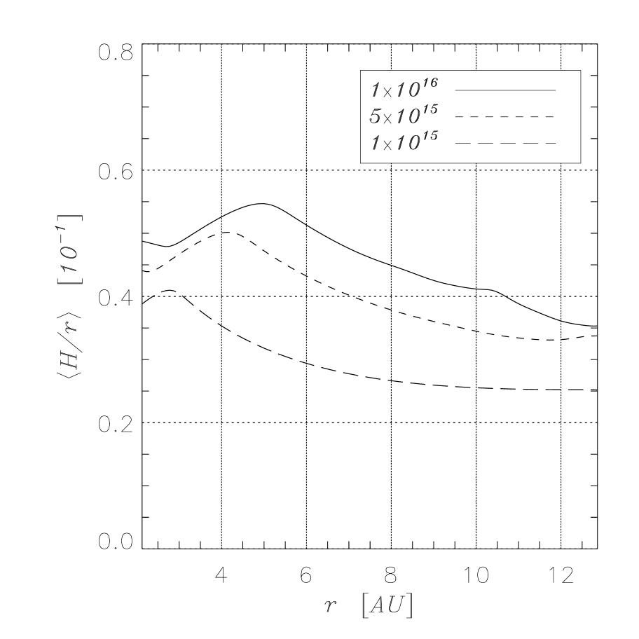
Figure 4: Some characteristics of radiative, unperturbed and stationary disks, as function of the magnitude of kinematic viscosity (shown in the legend in $\mathrm{cm}^{\mathrm{2}}\,\mathrm{s}^{\mathrm{-1}}$). Radial boundaries are closed in order to achieve a strict stationarity by preventing mass losses. Top left: Surface density. Top right: Midplane temperature. Bottom left: Disk effective temperature (eq. [11]). Bottom right: Disk aspect ratio.

Model parameterization deserves more attention in these computations than it did in the simulations where energy transfer by radiation is not taken into account. The reason for this resides in the nature of the opacity coefficient $\kappa$, that is always in cgs units. Hence, lengths and masses are to be fixed in physical units and consequently outcomes will not be scale-free, as they were in other circumstances (see, e.g., Paper I; Paper II).

As in previous simulations, we model a circumstellar disk, orbiting a one-solar-mass star ($\mbox{$M_{*}$}=1\;\mbox{$M_{\odot}$}$), whose radial borders are $r_{\mathrm{min}}=2\;\mbox{{AU}}$ and $r_{\mathrm{max}}=13\;\mbox{{AU}}$. The initial mass enclosed in this domain is $\mbox{$M_{\mathrm{D}}$}=4.8\times 10^{-3}\;\mbox{$M_{*}$}$, i.e., $0.01\;\mbox{$M_{*}$}$ within $20\;\mbox{{AU}}$ (D’Alessio et al., 1998). Since in stationary Keplerian disks, the energy budget is regulated by the balance between viscous dissipation and radiative losses (eq. [26]), the magnitude of viscosity may play an important role. Hence, we will cover various viscosity regimes. The bulk of the simulations were run with a constant kinematic viscosity coefficient, by setting $\nu=1.0\times 10^{15}$, $5.0\times 10^{15}$, and $1.0\times 10^{16}\;\mbox{$\mathrm{cm}^{\mathrm{2}}\,\mathrm{s}^{\mathrm{-1}}$}$ (Bell et al., 1997). Besides physical viscosity, we consider an artificial viscosity, which is active only in compression regions, according to the tensor formulation explained in § 2.4. The length $\mathcal{L}$ is chosen to be equal to the maximum grid spacing, on each grid level (Stone & Norman, 1992; Ziegler, 1998). The mean molecular weight is $\mu=2.39$ (Morfill, Tscharnuter, & Voelk, 1985) and the adiabatic index $\gamma=1.4$.

Figure 4 shows characteristic averaged quantities of non-perturbed, stationary disks with the aforementioned characteristics. To distinguish among the different viscosity (and temperature) disk regimes, models will be referred to as “Hot” (H), “Warm” (W), and “Cold” (C).

To further explore the parameter space, two models were executed applying the Shakura-Sunyaev viscosity prescription $\nu=\alpha\,c_{s}\,H$, with $\alpha=10^{-2}$ and $10^{-3}$ (models A2 and A3). Hence, in such models $\nu$ is a function of space and time.

An embedded planet is placed on a fixed circular orbit at $r_{\mathrm{p}}=5.2\;\mbox{{AU}}$. The azimuthal position of the planet is kept fixed ($\varphi_{\mathrm{p}}=\pi$) by the employment of a rotating grid. In order to obtain reliable outcomes in the two-dimensional geometry, we consider a planetary mass range extending from $\mbox{$M_{\mathrm{p}}$}=33\;\mbox{$M_{\oplus}$}$ to $\mbox{$M_{\mathrm{p}}$}=1\;\mbox{$M_{\mathrm{J}}$}$ or, in terms of mass ratios $q=\mbox{$M_{\mathrm{p}}$}/\mbox{$M_{*}$}$, we have models with $q=1\times 10^{-4},2\times 10^{-4},5\times 10^{-4}$, and $q=1\times 10^{-3}$. It has been recently demonstrated (Paper II) that, concerning gravitational torques and mass accretion, 3D models agree quite well with 2D ones in that mass range.

However, since the disk thickness is sufficiently small, even for low protoplanetary masses (see Fig. 4), we go as far as to simulate an additional C-model with $\mbox{$M_{\mathrm{p}}$}=20\;\mbox{$M_{\oplus}$}$. Figure 5 shows the disk semi-thickness in the planet’s neighborhood for three selected masses. Indicating with $R_{\mathrm{H}}=r_{\mathrm{p}}\,\left(q/3\right)^{1/3}$ the planet’s Hill radius, one can clearly see that the condition $H\lesssim R_{\mathrm{H}}$ locally holds even in the smallest mass case. The figure also shows that protoplanets dwell in cavities and thus radiation from the central star cannot directly reach the surrounding matter.

The smoothing length $\delta$ is set to $2\times 10^{-2}\,R_{\mathrm{H}}$ (see eq. [1]). All of the models are executed in an accreting and a non-accreting mode. When accretion onto the planet is allowed, the procedure outlined in Paper I is utilized. The accretion region has a radius $\kappa_{\mathrm{ac}}=0.1\,R_{\mathrm{H}}$, which should be short enough to let the whole accretion procedure be almost independent of the removal characteristic time, as proved by Tanigawa & Watanabe (2002).

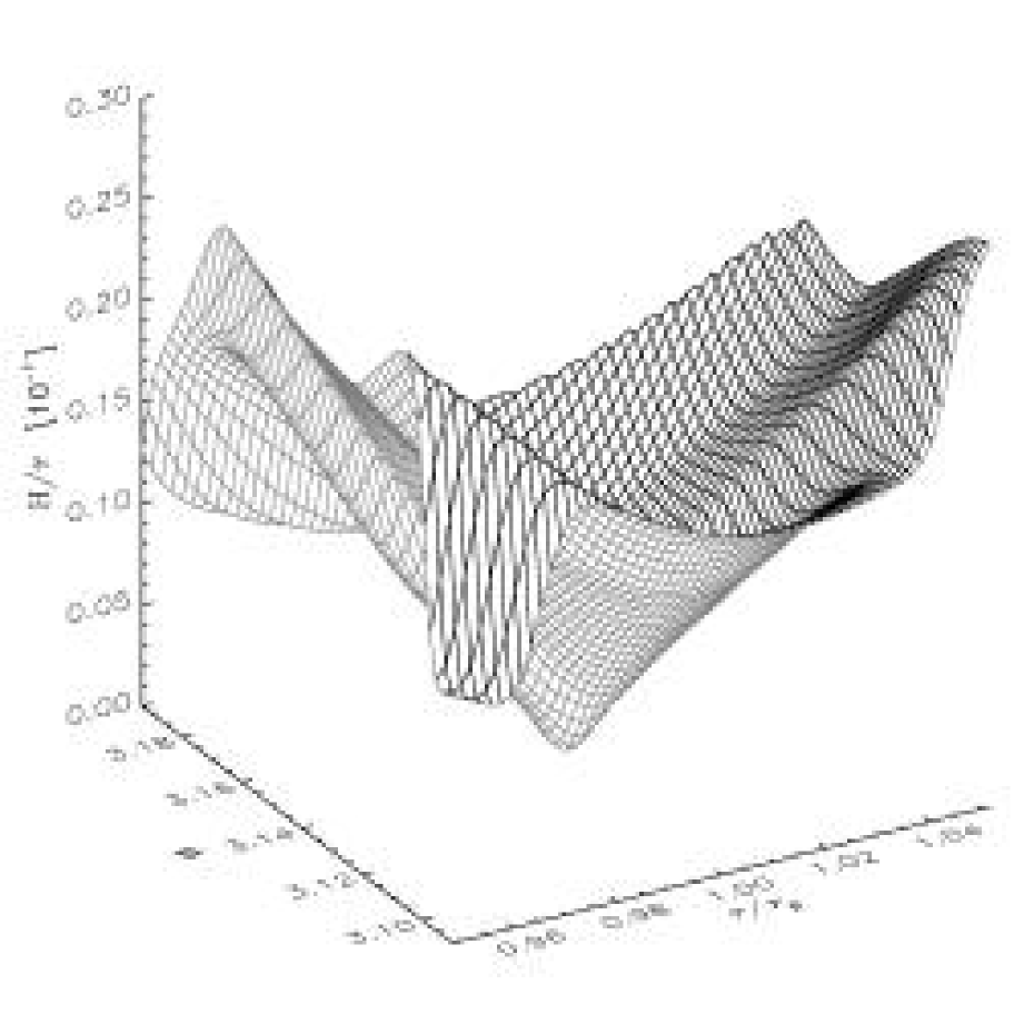
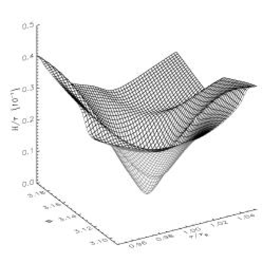
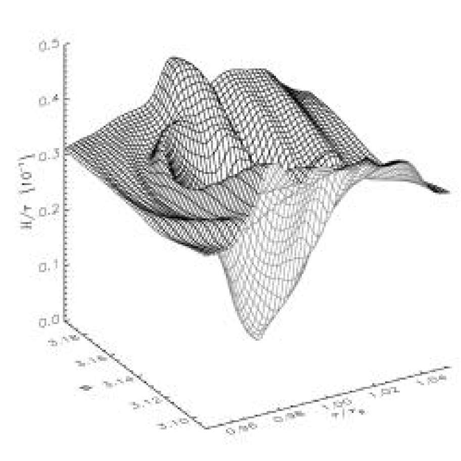
Figure 5: Because of the gravitational field of the embedded planet, the disk scale height may reduce considerably in its proximity, as prescribed by equation (19). This effect is shown here for models with different planetary masses: $\mbox{$M_{\mathrm{p}}$}=1\,\mbox{$M_{\mathrm{J}}$}$ with $\nu=1.0\times 10^{16}$ $\mathrm{cm}^{\mathrm{2}}\,\mathrm{s}^{\mathrm{-1}}$(left); $\mbox{$M_{\mathrm{p}}$}=0.1\,\mbox{$M_{\mathrm{J}}$}$ with $\nu=1.0\times 10^{16}$ $\mathrm{cm}^{\mathrm{2}}\,\mathrm{s}^{\mathrm{-1}}$(center); $\mbox{$M_{\mathrm{p}}$}=20\;\mbox{$M_{\oplus}$}$ with $\nu=1.0\times 10^{15}$ $\mathrm{cm}^{\mathrm{2}}\,\mathrm{s}^{\mathrm{-1}}$(right). For comparison, in the lowest mass case, $R_{\mathrm{H}}/r_{\mathrm{p}}=0.027$.

Figure 6 illustrates the influence of the extent of the domain’s radial extent for Jupiter C-models. Simulations provide quite consistent outcomes over the matching domain. Differences exist only close to the inner border, due to inflow boundary conditions.

Figure 6: Average surface density (left) and temperature (right) profiles belonging to two Jupiter-mass test models which differ only by the extension of the radial domain. The solid line refers to a model for which $r_{\mathrm{min}}=1.3\;\mbox{{AU}}$ and $r_{\mathrm{max}}=20.8\;\mbox{{AU}}$ ($\mbox{$M_{\mathrm{D}}$}=7.5\times 10^{-3}\;\mbox{$M_{*}$}$), whereas the dashed line represents a standard radial domain model $[2,13]\;\mbox{{AU}}$ ($\mbox{$M_{\mathrm{D}}$}=3.5\times 10^{-3}\;\mbox{$M_{*}$}$). The kinematic viscosity corresponds to that employed in C-models.

4.1 Initial and Boundary Conditions

Initial conditions require the assignment of the three functions $\Sigma(t=0)$, $T(t=0)$, and $\boldsymbol{u}(t=0)$ that we suppose to be axi-symmetric because we start from a stationary disk.

The theoretical surface density profile of a stationary accretion disk, with constant $\nu$, is a power-law of the radial distance $r$ (Lynden-Bell & Pringle, 1974), as also found numerically in § 3.1. Thus, as starting density distribution for our simulations, we set

$$\Sigma(t=0)=\Sigma_{0}\,\sqrt{\frac{r_{\mathrm{p}}}{r}}.$$ (33)

where $\Sigma_{0}$ is determined by the disk mass value $M_{\mathrm{D}}$.

Table 1: Initial Temperatures versus Viscosity and Disk Mass.

$\nu\;[\mbox{$\mathrm{cm}^{\mathrm{2}}\,\mathrm{s}^{\mathrm{-1}}$}]$	$T_{0}\;[\mbox{$\mathrm{K}$}]$	$T_{\mathrm{max}}\;[\mbox{$\mathrm{K}$}]$	$T_{\mathrm{min}}\;[\mbox{$\mathrm{K}$}]$
$1.0\times 10^{15}$	$50$	$180$	$13$
$5.0\times 10^{15}$	$110$	$235$	$22$
$1.0\times 10^{16}$	$150$	$295$	$26$

Note. — Values of the initial temperature as function the three values of the kinematic viscosity. Temperatures are sampled at $r=r_{\mathrm{p}}=5.2\;\mbox{{AU}}$ ($T_{0}$), $r=r_{\mathrm{max}}=2.1\;\mbox{{AU}}$ ($T_{\mathrm{max}}$), and $r=r_{\mathrm{min}}=13\;\mbox{{AU}}$ ($T_{\mathrm{min}}$). Models with $\alpha$-viscosity A2 and A3 are initiated as C-model.

Calculations carried out for different viscosity magnitudes imply different temperature regimes (see Fig. 4). According to them, the initial temperature distribution is prescribed. The behavior of the profiles in the top-right panel of Figure 4 can be roughly reproduced by the power-law

$$T(t=0)=T_{0}(\nu)\,\left(\frac{r_{\mathrm{p}}}{r}\right)^{1.8}.$$ (34)

The initial temperature at $r=r_{\mathrm{p}}$ is given in Table 1 for three values of $\nu$. Finally, the initial circumstellar flow $\boldsymbol{u}(t=0)$ is a Keplerian one, corrected for the grid rotation.

As for the boundary conditions, all models are run with a partially open inner radial border and a reflective outer one. Thus, matter is free to flow out of the computational domain, at $r=r_{\mathrm{min}}$, but the opposite is not allowed. This is the same expedient invoked in Paper I and Paper II to artificially mimic the mass accretion toward the central star and avoid spurious wave reflection at the inner domain edge, which is the closer to the planet. The flow field is Keplerian both at $r_{\mathrm{min}}$ and $r_{\mathrm{max}}$: $\boldsymbol{u}=[0,r\,(\Omega_{\mathrm{K}}-\Omega_{\mathrm{p}})]$.

4.2 Numerical Specifications

The basic computational mesh is made of $N_{r}\times N_{\varphi}=143\times 423$ cells, while sub-grid patches are $64\times 64$. All of the computations are based on a five-grid hierarchy. Thus, the finest resolution ranges from $1.3\times 10^{-2}\,R_{\mathrm{H}}$ (if $\mbox{$M_{\mathrm{p}}$}=1\;\mbox{$M_{\mathrm{J}}$}$) to $2.9\times 10^{-2}\,R_{\mathrm{H}}$ (if $\mbox{$M_{\mathrm{p}}$}=33\;\mbox{$M_{\oplus}$}$). Further details on numerical issues have been presented in Paper I and Paper II.

Despite we have not implemented a sophisticated energy transport treatment, these simulations take between 35 and 40% longer than those discussed in Paper I, for equal size grid hierarchies.

5 Global Model Properties

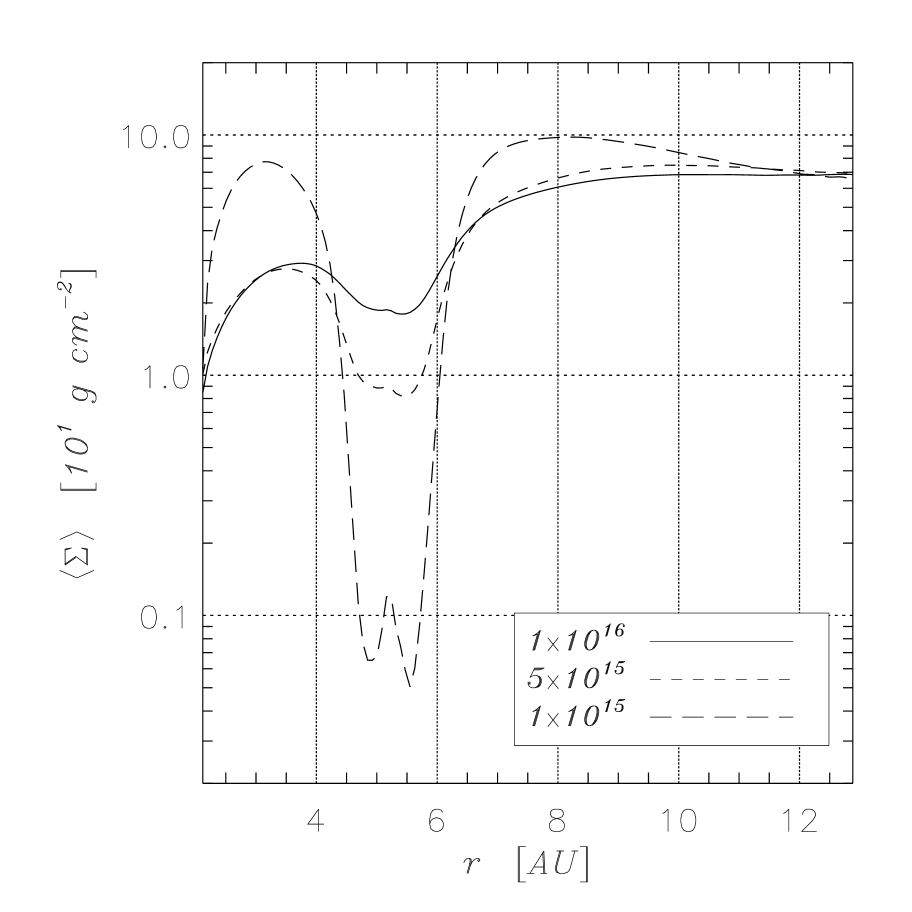
Figure 7: Average surface density (left) and temperature (right) in Jupiter-mass models after $240$ orbital periods. By this evolutionary time, models have settled on a quasi-equilibrium state. The different profiles refer to different values of $\nu$, as indicated in the legends. The density gap, in the C-model ($\nu=10^{15}$ $\mathrm{cm}^{\mathrm{2}}\,\mathrm{s}^{\mathrm{-1}}$), is more than an order of magnitude deeper (long-dash line) than it is in the other models. The temperature gap follows the same trend, though differences are smaller.

Figure 8: Average pressure scale-height (eq. [19]), normalized to the distance from the star, in Jupiter-mass models according to different viscosity values, as indicated in the legend (in $\mathrm{cm}^{\mathrm{2}}\,\mathrm{s}^{\mathrm{-1}}$).

We now examine the behavior of global quantities for some selected models because the large scale look of disks with planets is, observationally, of extreme importance. Figure 7 shows both the averaged surface density and temperature in Jupiter-mass computations with different kinematic viscosities. We note that matter (left panel) is more uniformly distributed in the H- (solid line) and W-model (short-dash line), with respect to the C-model (long-dash line). In these cases, the density gap is not very deep and actually looks like a depression, because of the larger viscosity coefficient and the depletion of the inner disk. On the one hand, in fact, a high viscosity prevents the formation of wide and deep gaps. On the other hand, a large viscosity facilitates the inner-disk depletion, since $\dot{M}_{\mathrm{D}}\propto\nu\,\Sigma$ (Lynden-Bell & Pringle, 1974). The disk depletion rate that we measure in these simulations ranges from few times $10^{-8}$ to $10^{-7}\,\mbox{$M_{\odot}$}\,\mathrm{yr}^{-1}$.

In contrast, in the low viscosity regime (C-model) a well-defined and deep gap is carved in, where the density is more than an order of magnitude lower than it is in the other two models. The density peak visible in the middle of the gap is the signature of the circumplanetary disk. Since material removed from gap regions is disposed at short distances, due to the small damping length of the waves launched by the planet, gap shoulders have high densities. It has been argued that these density enhancements might trigger planet formation. If so, low viscosity disks should be more efficient in doing that.

Following the reduction of thermal energy in the low density regions, a temperature gap accompanies the density gap (right panel, Fig. 7). In the C-model, temperatures drop below $20\;\mbox{$\mathrm{K}$}$ and it generally stays below $40\;\mbox{$\mathrm{K}$}$. As expectable, the temperature gap has a counterpart in the pressure scale height, as seen in Figure 8. Such a deep trough represents an additional evidence that, as long as an inner disk exists, protoplanets are shaded against stellar radiation.

Global views of both density and temperature 2D-distributions are displayed in Figure 9. Top panels illustrate the surface density, while the bottom ones show the temperature structure. From the density maps one can see that disk spirals get closer to each other toward the outer border of the domain. In fact, circumstellar spirals propagate at a velocity equal to the sound speed, which is proportional to $\sqrt{T}$ (see eq. [5]). Thus, the propagation velocity reduces as $r$ increases and therefore faster waves overtake slower ones. Past the gap region, temperature decays more rapidly in the C-model (Fig. 7, right panel), hence this phenomenon is more evident. From the bottom panels one can also deduce that spiral perturbations in the thermal energy and mass densities are quite phase coherent and thus disturbances in the thermal structure are rather weak.

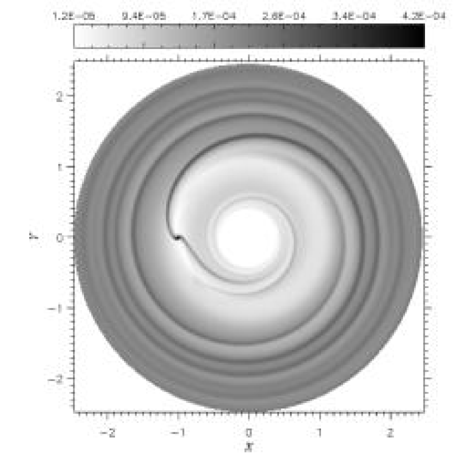
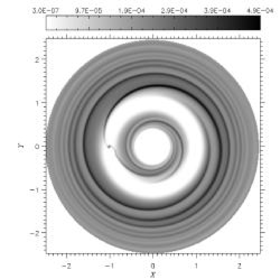
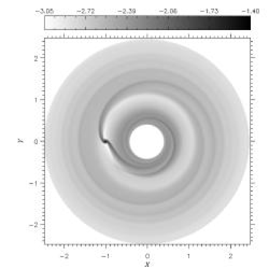
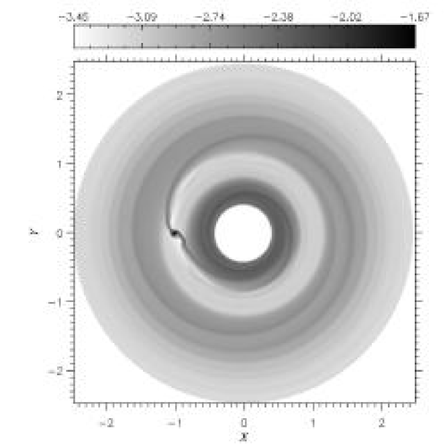
Figure 9: Two-dimensional surface density (top) and temperature (bottom) distributions for Jupiter-mass models. In the top panels, the color scale is linear; in the bottom ones the colors scale logarithmically. In this plot, $\Sigma=10^{-4}$ corresponds to $32.9\;\mbox{$\mathrm{g}\,\mathrm{cm}^{\mathrm{-2}}$}$, whereas $T=10^{-2}$ equals $198\;\mbox{$\mathrm{K}$}$. Left panels correspond to H-models whereas right panels refer to C models. Density distributions show clear evidences that the a well-defined gap needs a cold (i.e., low viscosity) environment to be established. The same consideration applies to the temperature distribution.

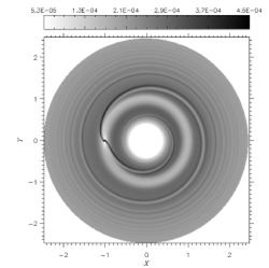
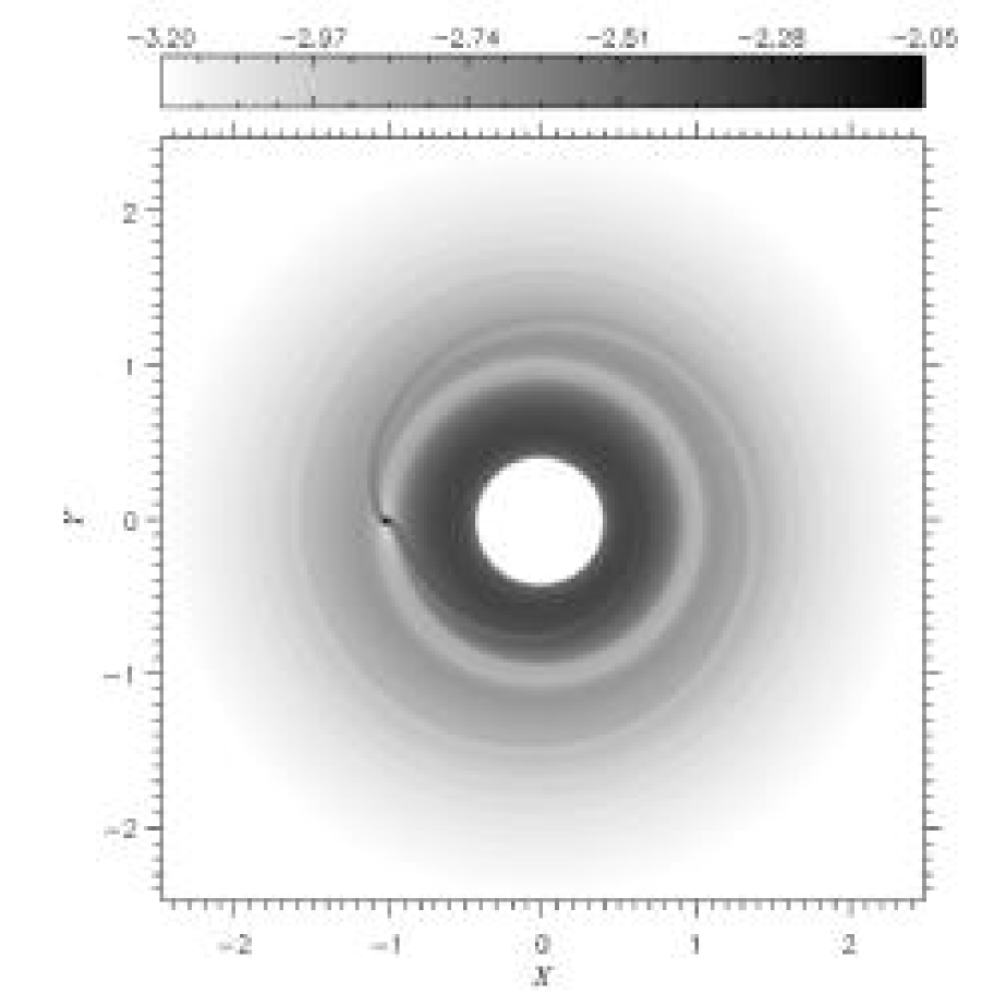
Figure 10: Left. Averaged surface density and temperature in C-models ($\nu=10^{15}$ $\mathrm{cm}^{\mathrm{2}}\,\mathrm{s}^{\mathrm{-1}}$) with different masses: $\mbox{$M_{\mathrm{p}}$}=0.5\;\mbox{$M_{\mathrm{J}}$}$ (solid line), $\mbox{$M_{\mathrm{p}}$}=0.2\;\mbox{$M_{\mathrm{J}}$}$ (short-dash line), and $\mbox{$M_{\mathrm{p}}$}=0.1\;\mbox{$M_{\mathrm{J}}$}$ (long-dash line). Right. 2D-distribution of the surface density (top) and temperature (bottom) of a C-model with $\mbox{$M_{\mathrm{p}}$}=0.1\;\mbox{$M_{\mathrm{J}}$}$. The density is scaled linearly, while temperature is scaled logarithmically. Conversion factors are: $\Sigma=10^{-4}\rightarrow 32.9\;\mbox{$\mathrm{g}\,\mathrm{cm}^{\mathrm{-2}}$}$, $T=10^{-2}\rightarrow 198\;\mbox{$\mathrm{K}$}$.

Shifting toward smaller masses, the gap is gradually refilled. This is visible in Figure 10, where C-models of different mass are compared. At $\mbox{$M_{\mathrm{p}}$}=0.1\;\mbox{$M_{\mathrm{J}}$}$ (i.e., $\mbox{$M_{\mathrm{p}}$}=33\;\mbox{$M_{\oplus}$}$), the gap is one order of magnitude as shallow as it is when $\mbox{$M_{\mathrm{p}}$}=0.5\;\mbox{$M_{\mathrm{J}}$}$. We will further address the issue of the gap structure in § 5.2, since gaps are considered promising features for detecting embedded planets. As regards the circumstellar disk spirals, only feeble traces are left, when $\mbox{$M_{\mathrm{p}}$}=0.1\;\mbox{$M_{\mathrm{J}}$}$, both in the temperature and density distributions. The absence of global disk features produced by an embedded body invalidates direct imaging observations as a detection tool in the intermediate-mass range, i.e., around a few times of Uranus’ mass.

Figure 11: Circumstellar disks are usually optically thick. This plot shows that this is generally the case even when a disk contains a Jupiter-mass body. The line sequence is the same as in Figure 7 (data refer to the same models). Left. Optical thickness averaged around the star. Only in the C-model, $\langle\tau\rangle$ drops below $1$. Right. Profiles at $\varphi\simeq 0$, i.e., $180^{\circ}$ away from the planet location. The medium becomes very optically thin ($\tau\ll 1$) only in the gap region of the C-model.

Concerning the emitted energy, we can notice that the optical thickness of the models is generally larger than one, throughout the computational domain (Fig. 11, left panel). The averaged $\tau$ stays above $1$ also at the outer disk edge. This is in agreement with what was found for accretion disks around T Tauri stars (D’Alessio et al., 1998). The density and temperature gap reflects in a similar feature in the distribution of $\tau$, as shown in Figure 11 (left panel). Nonetheless, even within the gap region, material is, on the average, optically thick ($\tau\gtrsim 1$). The exception is represented by the C-model, where gap optical thickness reaches values around $0.01$ at $\varphi=\varphi_{\mathrm{p}}+\pi$ (see Fig. 11, right panel). The most diluted portions of the gap, situated where the circumplanetary disk merges into the gap, have values of $\tau$ on the order of $10^{-2}$–$10^{-3}$.

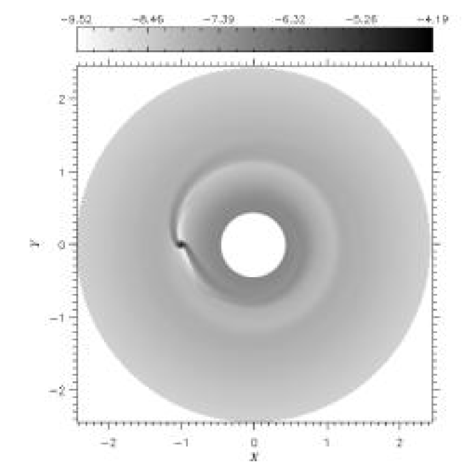
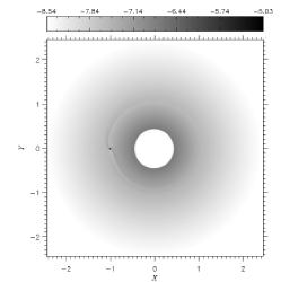
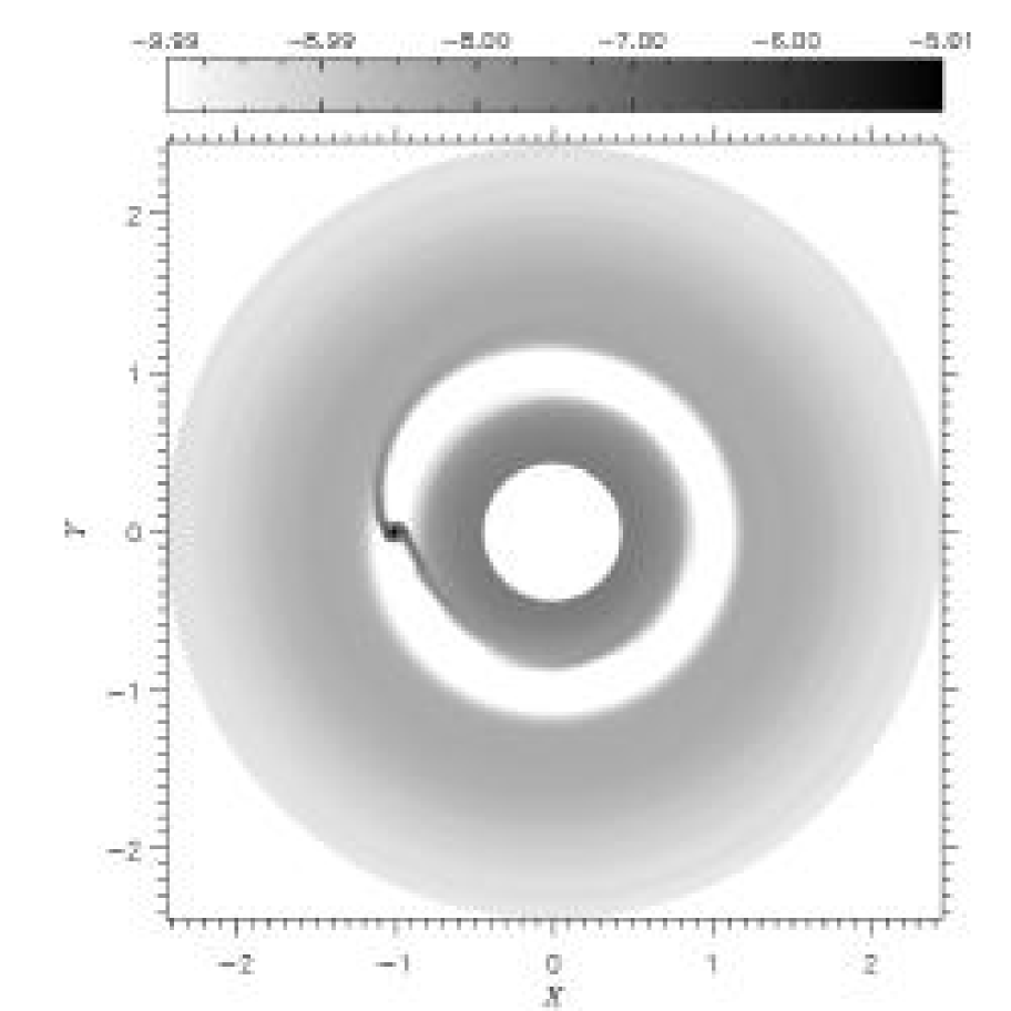
Figure 12: Flux radiated (i.e., $\Lambda$, see § 2.1 for details) by H-models (top) and C-models (bottom). Left panels regard simulations of Jupiter-mass objects, whereas right panels describe models with $\mbox{$M_{\mathrm{p}}$}=0.1\;\mbox{$M_{\mathrm{J}}$}$ ($\mbox{$M_{\mathrm{p}}$}=33\;\mbox{$M_{\oplus}$}$). The color scale in both panels is logarithmic. In plot units, $10^{-5}$ means an energy flux of $4.7\times 10^{4}\;\mathrm{erg}\,\mathrm{cm}^{-2}\,\mathrm{s}^{-1}$. For comparison, the surface flux of the Sun is $6.3\times 10^{10}\;\mathrm{erg}\,\mathrm{cm}^{-2}\,\mathrm{s}^{-1}$.

Finally, we examine the emitted flux $\Lambda$, computed according to equation (14) (see Fig. 12). From the observational point of view, disk gaps could represent a probe for protoplanet detection. In fact, this is by far the most extensive imprint that a planet leaves on a circumstellar disks. Prospective studies on observability of gaps due to Jupiter-mass protoplanets, have already been presented by Wolf et al. (2002); Steinacker & Henning (2003), and speculations on a developing gap around the T Tauri star TW Hya have been reported by Calvet et al. (2002). Here we do not intend to address the issue of whether gaps are really observable or to what extent they are. However, we have to notice that a necessary but not sufficient condition is that they must be wide, deep, and with sharp edges in order for the flux emitted from this region to have the strongest contrast with respect to the surrounding environment (Rice et al., 2003). From the bottom panels of Figure 12, it appears clear that low kinematic viscosities would favor this kind of investigation. Disk spirals are probably too elusive to be captured by present-day ground-based instruments, as shown by the flux maps. We also argue that it would seem rather unlikely to detect planetary masses smaller than Jupiter’s, by means of these measurements. Right panels of Figure 12 display the emitted flux in case of a $\mbox{$M_{\mathrm{p}}$}=0.1\;\mbox{$M_{\mathrm{J}}$}$ model. The quantity $\Lambda$ furnished by high-viscosity model (top) looks quite smooth and only some inhomogeneities appear in C-model (bottom).

5.1 Models with $\alpha$-viscosity

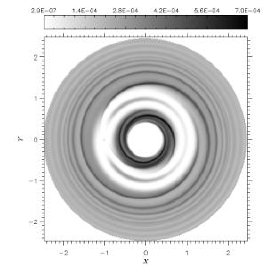
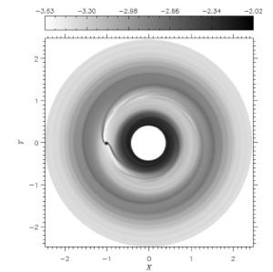
Figure 13: Left. Averaged surface density and temperature in the Jupiter-mass $\alpha$-viscosity models A3 ($\alpha=10^{-3}$, solid line) and A2 ($\alpha=10^{-2}$, long-dash line). Right. 2D-distribution of the surface density (top) and temperature (bottom) from models A3. The density scales linearly and temperature scales logarithmically. Conversion factors are: $\Sigma=10^{-4}\rightarrow 32.9\;\mbox{$\mathrm{g}\,\mathrm{cm}^{\mathrm{-2}}$}$, $T=10^{-2}\rightarrow 198\;\mbox{$\mathrm{K}$}$.

So far we have considered disks with a constant $\nu$. However, we have also investigated the effects of a different viscosity prescription, namely an $\alpha$-type viscosity (Shakura & Sunyaev, 1973). Two Jupiter-mass accreting models were run in this mode, one with $\alpha=10^{-2}$ (model A2) and the other with $10^{-3}$ (model A3). Such values are representative of those recently estimated by Papaloizou & Nelson (2003) and Winters, Balbus, & Hawley (2003) who performed MHD disk simulations, with embedded Jupiter-size bodies, and could therefore evaluate the stress parameter $\alpha$ in a self-consistent fashion. Indeed, referring to the constant viscosity models discussed above, by making the azimuthal mean $2\,\pi/\langle\alpha\rangle=(1/\nu)\,\int{c_{s}\,H\,\mathrm{d}\varphi}$, we get a value of $\langle\alpha\rangle$ ranging from $3\times 10^{-2}$ in the inner disk to $4\times 10^{-3}$ in the outer disk. Specifically, C-models yield an overall trend of $\langle\alpha\rangle$ which is the closest to $10^{-2}$. And in fact outcomes from $\alpha$-viscosity model A2 are not much different from those obtained from the Jupiter-mass C-model. The quantity $\langle\Sigma\rangle$ is very similar to that illustrated in left panel of Figure 7 (long-dashed line) whereas $\langle T\rangle$ is only slightly different (near the inner border) from the one in the right panel of the same Figure.

Some more important deviations from what has been seen thus far are instead encountered in the A3-model, as displayed in Figure 13. The averaged surface density shows a significant hump (top-left panel, solid line), inside the gap region, not observed in the other viscosity regimes. This is not caused by the mass accumulation around the planet but it is produced by   material   lingering   around Lagrangian points L4 and L5, as it appears from the ring-like traces in the middle of the density gap in the top-right panel Figure 13. This also appear to be a persistent feature, in fact no change is measured over the last 50 orbital periods. L4 and L5 points are equilibrium locations for the restricted three-body problem. Hence, one can expect that the thermal energy is larger near such points than anywhere else in the gap. In turn, viscous torques, which are enhanced by the locally increased kinematic viscosity are more efficient in contrasting gravitational torques. Thereby, material is more likely forced to evolve on the much longer viscous time scale $t_{\mathrm{vis}}\simeq r^{2}_{\mathrm{p}}/\nu=r_{\mathrm{p}}/(\alpha\,c_{s}\,h)$.

As for the temperature (Fig. 13, bottom panels), the largest discrepancies between models A2 and A3 occur toward the inner border.

5.2 Gaps as Planet Signatures

Table 2: Gap Occurrence and Depth.

	C-Models				H-Models
$\mbox{$M_{\mathrm{p}}$}/\mbox{$M_{\mathrm{J}}$}$	Acc.	Non-Acc.	N.F.		Acc.	Non-Acc.	N.F.
$1.0\phantom{0}$	$<0.01$	$<0.01$			$0.6$	$0.8$	X
$0.5\phantom{0}$	$\phantom{string}0.06$	$\phantom{string}0.2\phantom{0}$			$0.9$	NG	X
$0.2\phantom{0}$	$\phantom{string}0.3\phantom{0}$	$\phantom{string}0.4\phantom{0}$	X		NG	NG	X
$0.1\phantom{0}$	$\phantom{string}0.6\phantom{0}$	NG	X		NG	NG	X
$0.06$	$\phantom{string}0.8\phantom{0}$	NG	X				X

Note. — Ratio of the minimum density in the gap to the density at the gap’s taller shoulder (rounded to the first significant digit). Values are recovered from the azimuthal average of $\Sigma$ around the star. The letters “NG” stand for “No Gap”. The symbol “X” appear whenever at least one of criterion (35) and (36) is not fulfilled (N.F.).

We have seen in the previous two sections that the gap structure drastically depends on the viscosity regime. The standard criterion to open a gap in a disk requires two conditions (Lin & Papaloizou, 1985, 1993). The first is a thermal condition given by:

$$\left(\frac{\mbox{$M_{\mathrm{p}}$}}{\mbox{$M_{*}$}}\right)>3\,\left(\frac{H}{r}\right)^{3}=3\,h^{3},$$ (35)

i.e., the Roche lobe must be larger than the disk scale height. Because of planet’s gravity (see eq. [19]) and the low temperatures established in gap regions, this condition is always fulfilled when $\mbox{$M_{\mathrm{p}}$}\gtrsim 0.1\;\mbox{$M_{\mathrm{J}}$}$ (see Fig. 8). The second condition concerns the requirement that tidal torques exceed viscous torques and reads

$$\left(\frac{\mbox{$M_{\mathrm{p}}$}}{\mbox{$M_{*}$}}\right)>\left(\frac{40}{\mathcal{R}}\right),$$ (36)

where $\mathcal{R}=r^{2}\,\Omega_{\mathrm{K}}/\nu$ is the Reynolds number. The right hand side of equation (36) is proportional to $\nu$ and in our case goes from $\approx 4\times 10^{-3}$ (H-models) to $\approx 4\times 10^{-4}$ (C-models). Thereby, we should not obtain gaps in any of the H-models. Figure 7 (solid line) decently agrees with this prediction, since only a trough is dug in H-model. However, condition (36) is partly violated in the low-viscosity regime (Fig. 10), because a clear gap is visible for the $\mbox{$M_{\mathrm{p}}$}=0.2\;\mbox{$M_{\mathrm{J}}$}$ case and a trough appears for $\mbox{$M_{\mathrm{p}}$}=0.1\;\mbox{$M_{\mathrm{J}}$}$. In Table 2 we report the gap occurrence and depth for some of the models.

One reason why the above criterion could not properly apply to our calculations lies in the fact that it was derived for simple polytropic disks, while we simulate also the thermal evolution of the system. As implied by the profiles in the top-left panel of Figure 13, it is even harder to predict the gap presence when the kinematic viscosity depends on the local fluid temperature.

6 Circumplanetary Disks

The first distinction about the circumplanetary flow has to be made according to whether the planet is accreting or not. Therefore, we shall carry out separate discussions, based on H- and C-models, as well as $\alpha$-viscosity models A2 and A3.

6.1 Accreting Models

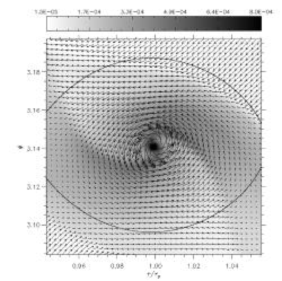
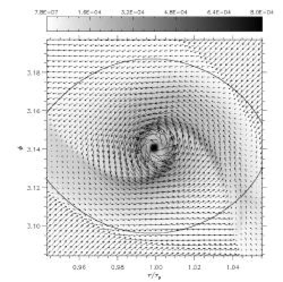
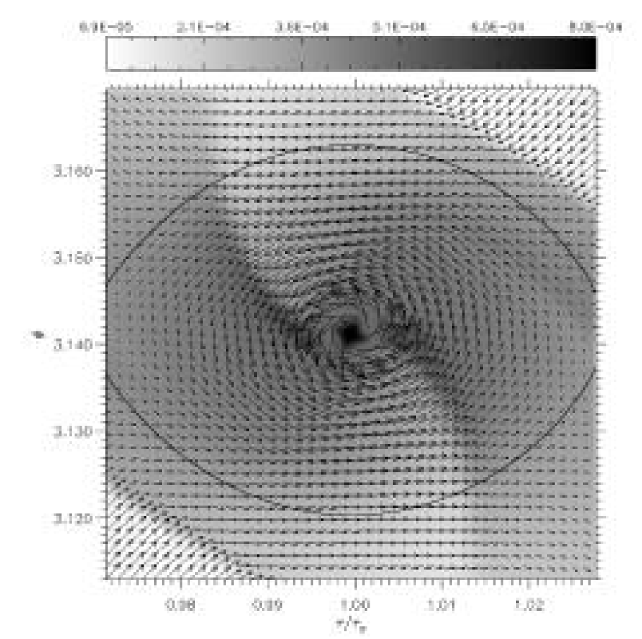
Figure 14: Density distribution and velocity field around $\mbox{$M_{\mathrm{p}}$}=1\;\mbox{$M_{\mathrm{J}}$}$ (top) and $\mbox{$M_{\mathrm{p}}$}=0.1\;\mbox{$M_{\mathrm{J}}$}$ (bottom) models. Right panels refer to H-models ($\nu=10^{16}\;\mbox{$\mathrm{cm}^{\mathrm{2}}\,\mathrm{s}^{\mathrm{-1}}$}$) whereas left ones refer to C-models ($\nu=10^{15}\;\mbox{$\mathrm{cm}^{\mathrm{2}}\,\mathrm{s}^{\mathrm{-1}}$}$). In each panel, color scales are linear. In the units used in the color bar, $10^{-4}$ corresponds to $\Sigma=32.9\;\mbox{$\mathrm{g}\,\mathrm{cm}^{\mathrm{-2}}$}$.

Figure 14 indicates that, inside of the Roche lobe, the general aspect of the flow circulation around $1\;\mbox{$M_{\mathrm{J}}$}$ and $0.1\;\mbox{$M_{\mathrm{J}}$}$ protoplanets resembles that obtained with local isothermal models in two dimensions (Paper I). However, specific characteristics of the flow do differ. A circumplanetary disk, extending over a fair fraction of Roche lobe, can be identified for both masses and viscosity regimes. The mass of such disks around one Jupiter-mass protoplanets, within the 80% of the Hill radius, is $1.03\times 10^{-5}\;\mbox{$M_{\mathrm{J}}$}$ in the H-model and $5.36\times 10^{-6}\;\mbox{$M_{\mathrm{J}}$}$ in the C-model. As regards calculations with $\mbox{$M_{\mathrm{p}}$}=0.1\;\mbox{$M_{\mathrm{J}}$}$ planets, the mass measured in the circumplanetary disk (or sub-disk, for brevity) of the C-model is $4.03\times 10^{-6}\;\mbox{$M_{\mathrm{J}}$}$, while the amount is nearly two times less in the H-model. While the flow dynamics in the Jupiter-mass model with $\alpha=10^{-2}$ (left panel in Fig. 15) is similar that of the C-model, the model with $\alpha=10^{-3}$ presents some peculiarities. As shown in right panel of Figure 15, the size of the circumplanetary disk is smaller than the Roche lobe. Moreover, the streams of matter associated with the spiral waves are narrower. The sub-disk mass measured in these cases is $3.9\times 10^{-6}\;\mbox{$M_{\mathrm{J}}$}$ (A2) and $1.5\times 10^{-6}\;\mbox{$M_{\mathrm{J}}$}$ (A3).

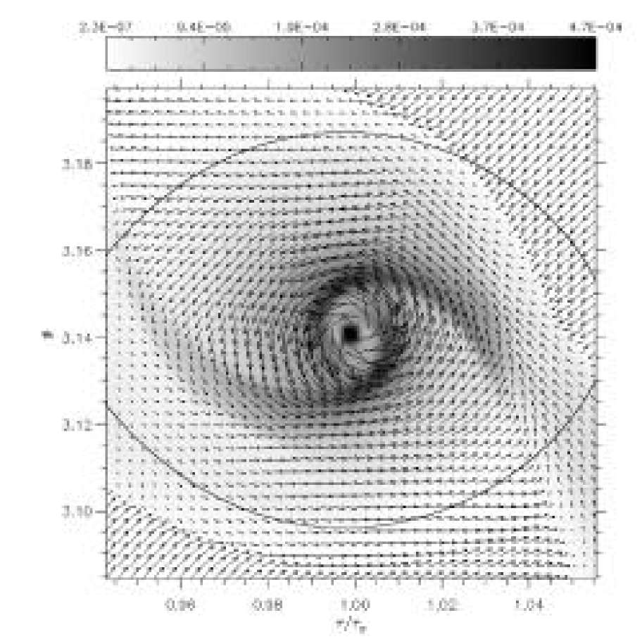
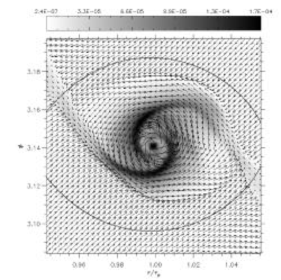
Figure 15: Density distribution and velocity field around the Jupiter-mass model in which the $\alpha$-viscosity prescription is used and set to $\alpha=10^{-2}$ (left) and $\alpha=10^{-3}$ (right). The color bar scale is linear and $10^{-4}$ is equal to $\Sigma=32.9\;\mbox{$\mathrm{g}\,\mathrm{cm}^{\mathrm{-2}}$}$.

The azimuthal average of the surface density distribution around the planet, inside the Roche lobe, can be fitted by a relation of the type (see Fig. 16):

$$\langle\Sigma\rangle\simeq\langle\Sigma\rangle_{0}\,\exp{\left[a_{1}\left(\frac{s}{R_{\mathrm{H}}}\right)\right]},$$ (37)

where $s/R_{\mathrm{H}}\leq 1$ and larger than a threshold length (either $0.1$ or $0.2\;R_{\mathrm{H}}$). The values of $\langle\Sigma\rangle_{0}$ and $a_{1}$ are reported in Table 3.

Table 3: Fit Parameters for the Averaged Surface Density.

	C-Models				H-Models
$\mbox{$M_{\mathrm{p}}$}/\mbox{$M_{\mathrm{J}}$}$	$\langle\Sigma\rangle_{0}\;[\mbox{$\mathrm{g}\,\mathrm{cm}^{\mathrm{-2}}$}]$	$a_{1}$	Range		$\langle\Sigma\rangle_{0}\;[\mbox{$\mathrm{g}\,\mathrm{cm}^{\mathrm{-2}}$}]$	$a_{1}$	Range
$1.0\phantom{0}$	$2.92\times 10^{2}$	$-4.4$	$[0.2,1.0]\,R_{\mathrm{H}}$		$2.14\times 10^{2}$	$-2.3$	$[0.2,1.0]\,R_{\mathrm{H}}$
$0.5\phantom{0}$	$1.59\times 10^{2}$	$-2.0$	$[0.2,1.0]\,R_{\mathrm{H}}$		$1.35\times 10^{2}$	$-1.3$	$[0.2,1.0]\,R_{\mathrm{H}}$
$0.2\phantom{0}$	$2.32\times 10^{2}$	$-1.5$	$[0.1,1.0]\,R_{\mathrm{H}}$		$8.57\times 10^{1}$	$-0.5$	$[0.1,1.0]\,R_{\mathrm{H}}$
$0.1\phantom{0}$	$1.99\times 10^{2}$	$-0.9$	$[0.1,1.0]\,R_{\mathrm{H}}$		$6.75\times 10^{1}$	$-0.2$	$[0.2,1.0]\,R_{\mathrm{H}}$
$0.06$	$1.47\times 10^{2}$	$-0.4$	$[0.2,1.0]\,R_{\mathrm{H}}$
	A3-Model				A2-Model
$1.0\phantom{0}$	$1.80\times 10^{2}$	$-7.5$	$[0.2,0.8]\,R_{\mathrm{H}}$		$2.36\times 10^{2}$	$-5.0$	$[0.2,1.0]\,R_{\mathrm{H}}$

Note. — Parameters that enter equation (37). This represents a linear best-fit of the logarithm of the averaged density $\langle\Sigma\rangle$ over the specified interval.

The presence of spiral features in the density distribution is an indication that the circumplanetary flow is Keplerian-like. Indeed, decomposing the velocity field $\boldsymbol{u}$ into the in-fall velocity (toward the planet) $w_{\mathrm{in}}$ and the rotational velocity (counter-clockwise around the planet) $w_{\mathrm{rot}}$, it turns out that the former is more than an order of magnitude less than the latter. In Jupiter-mass models, the rotational velocity within $0.5\,R_{\mathrm{H}}$ of the planet drops approximately as $s^{-0.6}$, nearly independently of the viscosity regime investigated in these computations. For $0.1\;\mbox{$M_{\mathrm{J}}$}$ models, this ratio declines at a slightly higher rate. Consequently, for $s\in[0.1,0.5]\,R_{\mathrm{H}}$, the ratio of $w_{\mathrm{rot}}$ to the local Keplerian velocity is always larger than $0.7$.

Comparing the right panels (C-models) of Figure 14 to Figure 13 (top and middle right panels) in Paper I, one can clearly see that spiral perturbations are less intense, as we show below, and more open. The latter circumstance is related to the lower values of the Mach number in the circumplanetary flow, which governs the inclination of the spiral wave with respect to the direction of the rotational motion. In fact, in local isothermal models $\mathcal{M}_{\mathrm{iso}}\simeq\sqrt{q\,(r_{\mathrm{p}}/s)}/h$. If $\mbox{$M_{\mathrm{p}}$}=1\;\mbox{$M_{\mathrm{J}}$}$, $\mathcal{M}_{\mathrm{iso}}$ drops from $\approx 8$, at $s=0.1\,R_{\mathrm{H}}$, to $2$, at $s=1\,R_{\mathrm{H}}$. As comparison, in the circumplanetary disk displayed in the upper-left panel of Figure 14, $\mathcal{M}$ lies between $2.4$ and $1.4$, whereas the low viscosity Jupiter-model (upper-right panel) provides values between $3$ and $1.5$. Models A2 and A3 yield similar values. The main reason for this difference resides in the larger value of the sound speed. Hence, perturbations can travel faster and are less distorted by the background motion of the flow. In the Jupiter-mass cases, illustrated in Figure 14, the azimuthally averaged $\mathcal{M}$ is approximately proportional to either $\sim s^{-0.1}$ (H-model) or to $\sim s^{-0.2}$ (C-model). In the limit of a nearly constant Mach number, wave perturbations assume the form of Archimedes’ spirals.

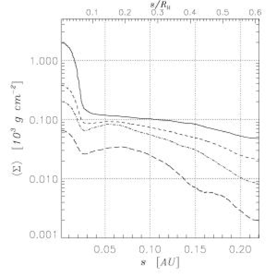
Figure 16: Surface density averaged around $\mbox{$M_{\mathrm{p}}$}=1\,\mbox{$M_{\mathrm{J}}$}$ planets in the inner part of the Roche lobe. Considered models are H (solid line), C (short-dash line), A2 (Dash-dot line), and A3 (long-dash line).

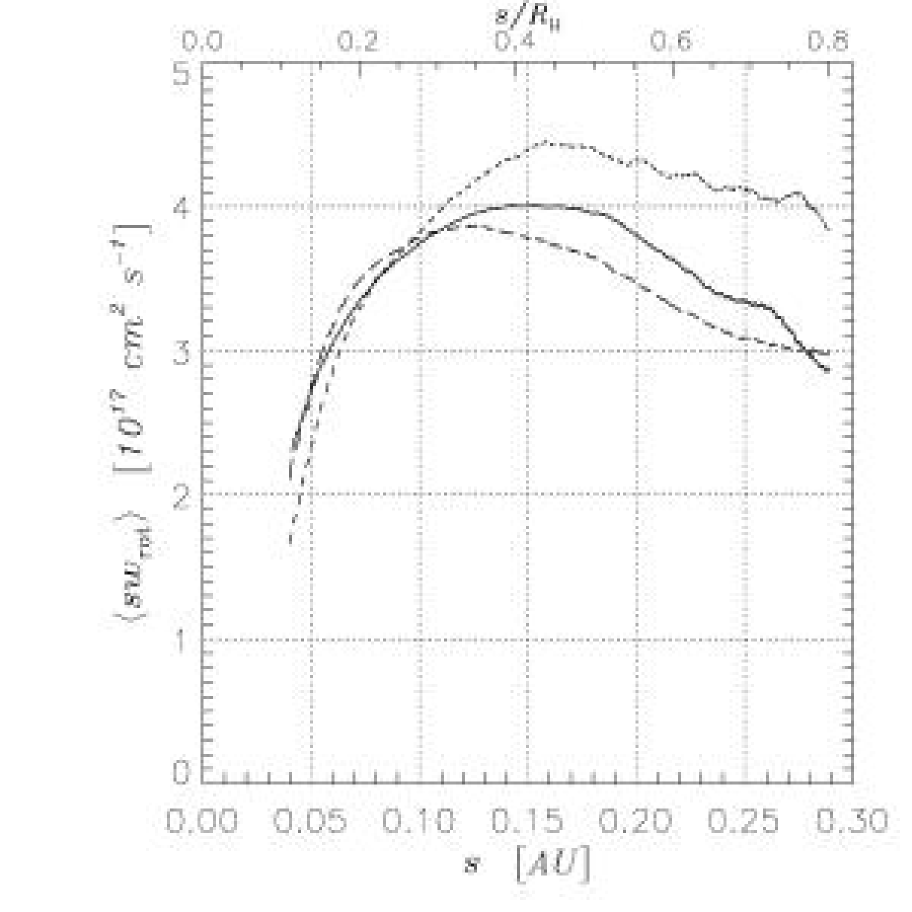
Figure 17: Specific angular momentum ($s\,w_{rot}$), averaged around $\mbox{$M_{\mathrm{p}}$}=1\,\mbox{$M_{\mathrm{J}}$}$ planets modeled with different geometries and thermal structures. The solid line belongs to the 2D C-model presented in this paper. The short-dash line derives from a locally isothermal 2D model ($T\simeq 90\;\mbox{$\mathrm{K}$}$) as described in Paper I. The long-dash line comes from a locally isothermal 3D model ($T\simeq 90\;\mbox{$\mathrm{K}$}$) presented in Paper II. In this last case, the specific angular momentum is evaluated in the disk midplane ($z=0$).

As pointed out in Paper II, in a three-dimensional space circumplanetary spirals are weakened (see also Bate et al., 2003). In fact, because of the flow circulation above the disk midplane (see Paper II, Figure 3, middle and bottom panels), less angular momentum is carried inside the Roche lobe by the midplane flow. As anticipated above, the spiral density features look smoother in the models presented here. This is quantitatively demonstrated in Figure 17. In the Figure the average specific angular momentum $s\,w_{\mathrm{rot}}$ obtained from the $\mbox{$M_{\mathrm{p}}$}=1\;\mbox{$M_{\mathrm{J}}$}$ C-model (solid line) is compared to that of a 2D Jupiter-mass local-isothermal model (short-dash line) and to that of a 3D Jupiter-mass model from Paper II (long-dash line), which also assumes a quasi-isothermal gas around the planet. In the 3D case, the quantity $s\,w_{\mathrm{rot}}$ is computed at $z=0$, i.e., in the disk midplane. The latter two models are quasi-isothermal in the sense that the temperature distribution is fixed and depends only on the distance distance from the star $r$ according to the relation $T\propto(\mu/\gamma)\,h^{2}\,\mbox{$M_{*}$}/r$. Thus, around the planet’s location $r=r_{\mathrm{p}}$, $T\approx 90\;\mbox{$\mathrm{K}$}$ if the disk aspect ratio $h$ is $0.05$, $\mu=2.39$, and $\gamma=1.4$. From Figure 17 one can see that in the outer part of the Roche lobe ($s\gtrsim 0.3\;R_{\mathrm{H}}$), where spiral perturbations are strongest, the discrepancy between the two quasi-isothermal models lies between 20 and 30%, whereas the two-dimensional thermal model provides a specific angular momentum only 10% larger than that of the three-dimensional quasi-isothermal model. This occurrence can be attributed to the better pressure structure achieved by the calculations that account for the thermal energy budget.

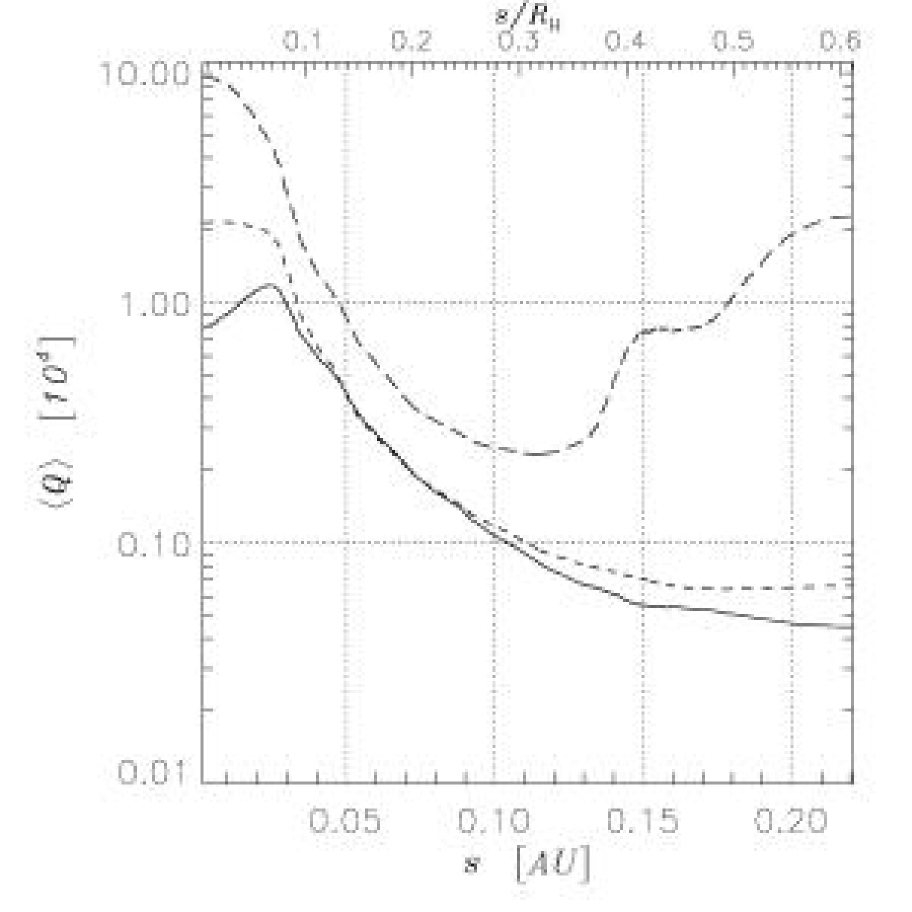
Figure 18: Toomre parameter $Q=c_{s}\,w_{rot}/(\pi\,G\,s\,\Sigma)$ averaged around $\mbox{$M_{\mathrm{p}}$}=1\,\mbox{$M_{\mathrm{J}}$}$ bodies in models H (solid line), C (short-dash line), and A3 (long-dash line). The large value of $\langle Q\rangle$ implies that circumplanetary disks around Jupiter-mass planets are gravitationally stable.

Circumplanetary disks should not suffer from gravitational instabilities since the Toomre parameter $Q$ is orders of magnitude larger than unity, as proved by Figure 18. This arises from the small value of the ratio between the mass of the circumplanetary disk and that of the planet.

Two-dimensional temperature distributions are rather symmetric with respect to the planet’s position, though they are marked by weak spiral perturbations. Figure 19 (top panels) shows the azimuthal averaged temperature around protoplanet with $\mbox{$M_{\mathrm{p}}$}=1\;\mbox{$M_{\mathrm{J}}$}$ (left) and $\mbox{$M_{\mathrm{p}}$}=0.1\;\mbox{$M_{\mathrm{J}}$}$ (right). In the Jupiter-mass case, maximum temperatures range from roughly $1500$ to $1000\;\mbox{$\mathrm{K}$}$, whereas $T$ reaches the value of the ambient medium ($\lesssim 50\;\mbox{$\mathrm{K}$}$) toward the border of the Hill sphere. Comparing H- and C-models, one can realize that the average temperature in the inner part of the Roche lobe differ by less than a factor two, whereas the $\alpha$-viscosity model A3 shows significant lower temperatures. In the low-mass case ($\mbox{$M_{\mathrm{p}}$}=0.1\;\mbox{$M_{\mathrm{J}}$}$), the peak temperature is around $1000\mbox{$\mathrm{K}$}$ and between $\approx 80$ and $\approx 40\;\mbox{$\mathrm{K}$}$ at $s=R_{\mathrm{H}}$, respectively for both H- and C-model. The average temperature differs by less than $\approx 30\;\mbox{$\mathrm{K}$}$ (Fig. 19, upper-right panel).

Over the entire sub-disk domain, $\langle T\rangle$ can be well fitted by the curve:

$$\langle T\rangle\simeq\langle T\rangle_{\bar{s}}\,\left(\frac{\bar{s}}{s}\right)^{\xi},$$ (38)

in which the length $\bar{s}$ is set to $0.1\,R_{\mathrm{H}}$, for convenience. Fitting parameters are reported in Table 4, together with the validity range of the fitting function. From entries in the Table, it turns out that the temperature generally falls off as $1/s$.

Table 4: Fit Parameters for the Averaged Temperature Distribution: Accreting Models.

	C-Models				H-Models
$\mbox{$M_{\mathrm{p}}$}/\mbox{$M_{\mathrm{J}}$}$	$\langle T\rangle_{\bar{s}}\;[\mbox{$\mathrm{K}$}]$	$\xi$	Range		$\langle T\rangle_{\bar{s}}\;[\mbox{$\mathrm{K}$}]$	$\xi$	Range
$1.0\phantom{0}$	$5.405\times 10^{2}$	$0.97$	$[0.05,1.0]\,R_{\mathrm{H}}$		$9.534\times 10^{2}$	$0.96$	$[0.1,1.0]\,R_{\mathrm{H}}$
$0.5\phantom{0}$	$5.304\times 10^{2}$	$0.96$	$[0.05,1.0]\,R_{\mathrm{H}}$		$8.425\times 10^{2}$	$0.95$	$[0.1,1.0]\,R_{\mathrm{H}}$
$0.2\phantom{0}$	$5.713\times 10^{2}$	$1.12$	$[0.05,1.0]\,R_{\mathrm{H}}$		$6.713\times 10^{2}$	$0.90$	$[0.05,1.0]\,R_{\mathrm{H}}$
$0.1\phantom{0}$	$4.395\times 10^{2}$	$1.03$	$[0.05,1.0]\,R_{\mathrm{H}}$		$4.868\times 10^{2}$	$0.79$	$[0.05,1.0]\,R_{\mathrm{H}}$
$0.06$	$4.634\times 10^{2}$	$1.07$	$[0.05,1.0]\,R_{\mathrm{H}}$
	A3-Model				A2-Model
$1.0\phantom{0}$	$2.484\times 10^{2}$	$1.04$	$[0.05,0.8]\,R_{\mathrm{H}}$		$4.234\times 10^{2}$	$0.95$	$[0.1,1.0]\,R_{\mathrm{H}}$

Note. — Parameters that enter equation (38). This is a linear best-fit of $\log{\langle T\rangle}$, computed inside of the Hill sphere. The column “Range” refers to the validity range of the fit.

Bottom panels of Figure 19 display the average effective temperature $\langle T_{\mathrm{eff}}\rangle$ (see eq. [11]) in the vicinity of protoplanets. Figure 20 shows that the magnitude of the optical thickness $\langle\tau\rangle$ is between $10$ and $100$, hence equation (14) yields $T_{\mathrm{eff}}\approx T/\tau^{0.25}$ and thus there is, at most, a factor three between the two temperatures. It should be noted that only the model A3 presents optically thin regions toward the edges of the sub-disk.

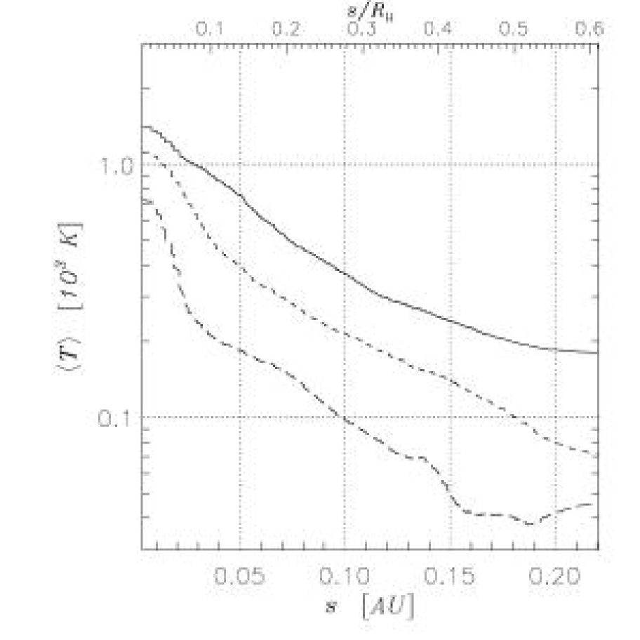
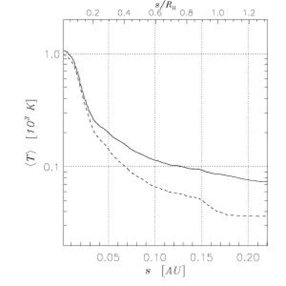
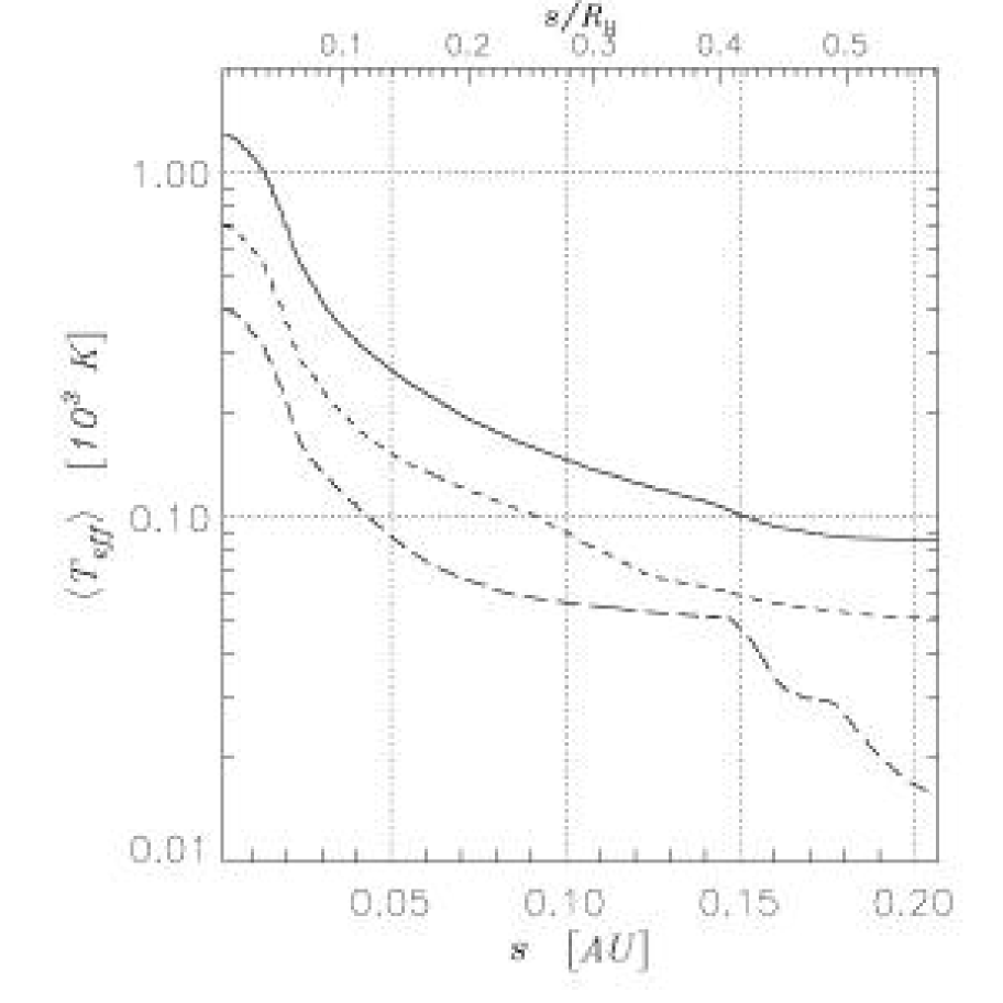
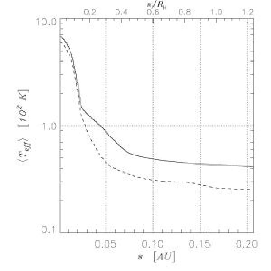
Figure 19: Azimuthally averaged temperature (top) and effective temperature (bottom) distribution, around Jupiter-size (left) and $0.1\;\mbox{$M_{\mathrm{J}}$}$ (right) accreting models. Solid, short-dash, and long-dash lines refer to models H, C, and A3, respectively.

Accreted matter also contributes to the energy budget of the circumplanetary disk via dissipation of gravitational energy into heat. This source of energy is not treated explicitly in these simulations. However, it is considered implicitly as a compression work term arising from the removal of matter in the accreting region. Tanigawa & Watanabe (2002) assumed the dissipation of gravitational energy as the only heating source and derived temperature profiles of sub-disks with different sound-speed regimes, performing local simulations with an isothermal equation of state. They found that the temperature would scale as $1/\sqrt{s}$, independently of the planetary mass.

We have to point out that, since radial transport of radiation is not treated here, one should expect large temperature gradients to be smoothed out. But we have seen that temperature profiles are not extremely steep, in the range of distances covered by these models, hence correction by radial transfer should not be dramatically relevant, as we are going to demonstrate.

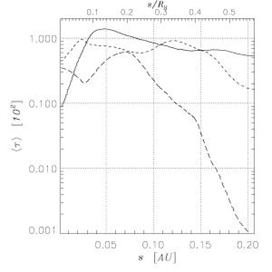
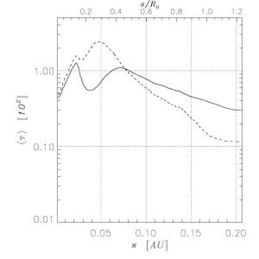
Figure 20: Average optical thickness around $\mbox{$M_{\mathrm{p}}$}=1\;\mbox{$M_{\mathrm{J}}$}$ (left) and $\mbox{$M_{\mathrm{p}}$}=0.1\;\mbox{$M_{\mathrm{J}}$}$ (right) protoplanets. The solid, short-dash, and long-dash lines reproduce the H-, C-, and A3-model, respectively.

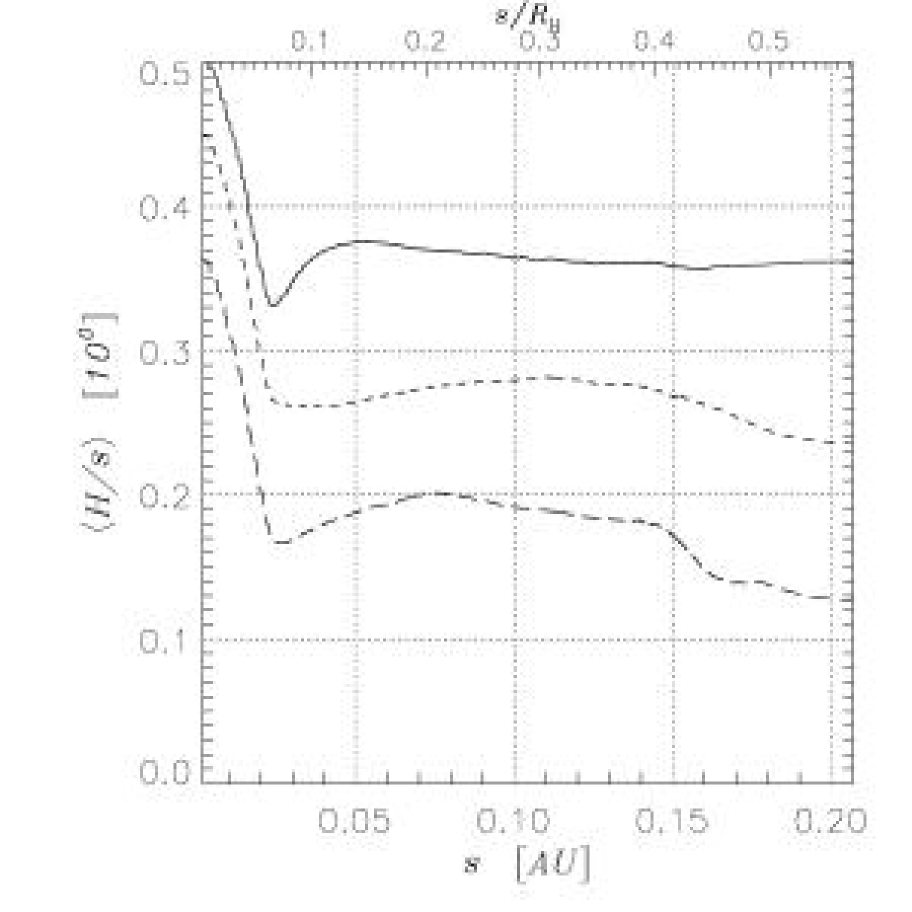
Figure 21: Average circumplanetary disk aspect ratio around $\mbox{$M_{\mathrm{p}}$}=1\;\mbox{$M_{\mathrm{J}}$}$ protoplanets. The solid, short-dash, and long-dash lines reproduce the H-, C-, and A3-model, respectively.

6.1.1 Radial Radiation Transfer in Circumplanetary Disks

Since the temperature gradient in the vicinity of a protoplanet may be quite steep, one of the hypothesis used in § 2.1 might locally break down. We refer to the assumption that the radiative flux in the vertical direction overwhelms those in the horizontal direction. With a semi-analytical analysis it is possible to make an a posteriori check of that hypothesis and shed some light over this matter. For simplicity we will suppose that the temperature distribution has a cylindrical symmetry around the planet, which is indeed what is observed in all of the models. Hence the total flux of energy transferred via radiation is

$$\Lambda\simeq\int_{-\infty}^{+\infty}\frac{\partial F_{z}}{\partial z}\,\mathrm{d}z+\int_{-\infty}^{+\infty}\frac{1}{s}\frac{\partial}{\partial s}[s\,F_{s}]\,\mathrm{d}z=\Lambda_{z}+\Lambda_{s},$$ (39)

where $s$ is the distance from the planet. The two terms on the right-hand side can be written as

$$\Lambda_{z}\simeq-\frac{128\,\sigma_{\mathrm{R}}}{3\,\kappa\,\rho}\,\frac{T^{4}}{H},$$ (40)

and

$$\Lambda_{s}\simeq-\xi^{2}\,\frac{128\,\sigma_{\mathrm{R}}}{3\,\kappa\,\rho}\,H\,\frac{T^{4}}{s^{2}}.$$ (41)

Equation (40) was obtained by setting $\partial T/\partial z\approx T/H$ in equation (39), whereas equation (41) was derived by adopting equation (38), which we have checked to hold as long as $\bar{s}\lesssim s\leq R_{\mathrm{H}}$. The validity of the relation (9), namely that $\Lambda\simeq\Lambda_{z}$, depends on the ratio of the left-hand sides of equations (40) and (41):

$$\frac{\left|\Lambda_{s}\right|}{\left|\Lambda_{z}\right|}=\xi^{2}\,\left(\frac{H}{s}\right)^{2}.$$ (42)

According to equation (42), only when $H<s$ the radiative cooling (eq. [14]) included in the energy equation is also locally a good approximation. As shown in Figure 21, this seems indeed to be the case in models involving Jupiter-size planets. To cast the above ratio in a more explicit form, one can use the expression for $H$ (eq. [19]) in the limit $s\ll r$, which yields

$$\left(\frac{H}{s}\right)^{2}=\frac{c_{s}^{2}}{\gamma}\,\left(\frac{s}{G\,\mbox{$M_{\mathrm{p}}$}}\right).$$ (43)

By using the form of the sound speed in equation (5), one gets

$$\left(\frac{H}{s}\right)^{2}=\left(\frac{k\,T}{\mu\,m_{\mathrm{H}}}\right)\,\left(\frac{s}{G\,\mbox{$M_{\mathrm{p}}$}}\right).$$ (44)

Therefore, because of the assumption made above on the temperature profile, equation (42) becomes

$$\frac{\left|\Lambda_{s}\right|}{\left|\Lambda_{z}\right|}=\xi^{2}\,\left(\frac{k\,\langle T\rangle_{\bar{s}}}{\mu\,m_{\mathrm{H}}}\right)\,\left(\frac{\bar{s}}{G\,\mbox{$M_{\mathrm{p}}$}}\right)\,\left(\frac{\bar{s}}{s}\right)^{\xi-1}.$$ (45)

Since the distance $s$ is constrained by the applicability range of equation (38), the ratio given by equation (45) is supposedly meaningful roughly for $s\in[0.1\,R_{\mathrm{H}},R_{\mathrm{H}}]$, for the models considered here. With the appropriate values, the ratio (45) becomes

$$\frac{\left|\Lambda_{s}\right|}{\left|\Lambda_{z}\right|}=0.145\,\xi^{2}\left(\frac{\langle T\rangle_{\bar{s}}}{1000\,\mbox{$\mathrm{K}$}}\right)\left(\frac{\mbox{$M_{\mathrm{J}}$}}{\mbox{$M_{\mathrm{p}}$}}\right)^{2/3}\left(\frac{\bar{s}}{s}\right)^{\xi-1}.$$ (46)

Equation (46) is an evaluation of equation (45) at a distance $s$ from the planet, whose length shortens as $\mbox{$M_{\mathrm{p}}$}^{1/3}$. Since the squared sub-disk aspect ratio grows as $1/\mbox{$M_{\mathrm{p}}$}$, the flux ratio goes as $\mbox{$M_{\mathrm{p}}$}^{2/3}$. From Table 4, we see that $|\xi-1|$ is between $0.03$ and $0.12$ in C-models and between $0.04$ and $0.21$ in H-models. Therefore, the right-most term in equation (46) can be considered as a unity term. Thus, around $s\approx\bar{s}=0.1\,R_{\mathrm{H}}$, $\left|\Lambda_{s}\right|/\left|\Lambda_{z}\right|=0.13$ for the Jupiter-mass H-model and a factor two as small for the C-model. Similar small numbers are obtained from both the A2 and A3 model. For $\mbox{$M_{\mathrm{p}}$}/\mbox{$M_{\mathrm{J}}$}=0.1$, the ratio increases, respectively, to $0.2$ and $0.3$, which is consistent with the applicability limit of the two-dimensional approximation. Thereby, apart from regions closer than $\sim 0.1\;R_{\mathrm{H}}$ to the accreting planet which, probably, cannot be properly investigated by these computations, radiation transport in the radial direction does not play a major role in the energy budget of circumplanetary disk material. This is in agreement with the standard scenario of the late stages of protojovian disks (e.g., Coradini et al., 1989; Canup & Ward, 2002).

6.2 Non-accreting Models

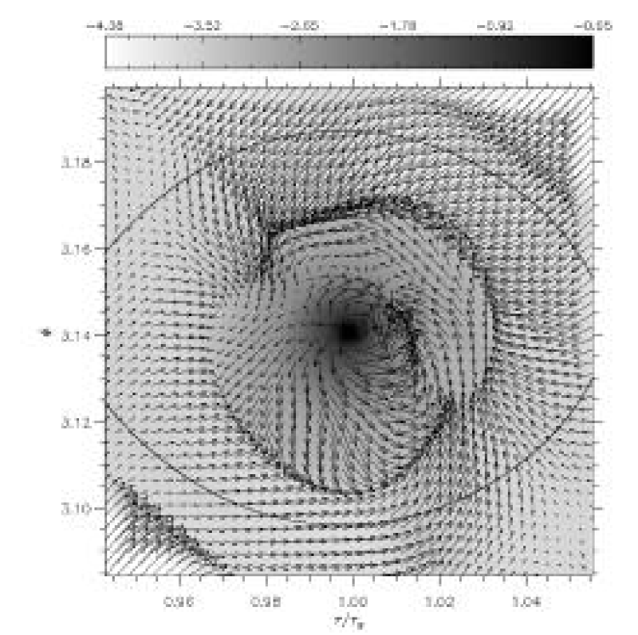
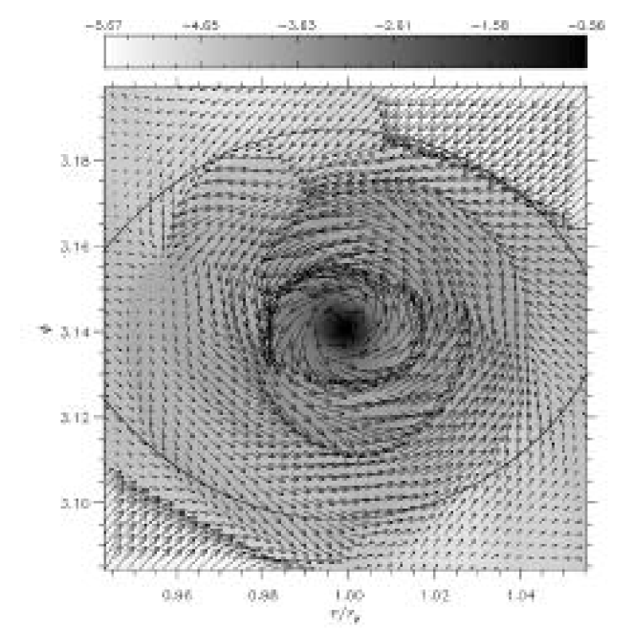
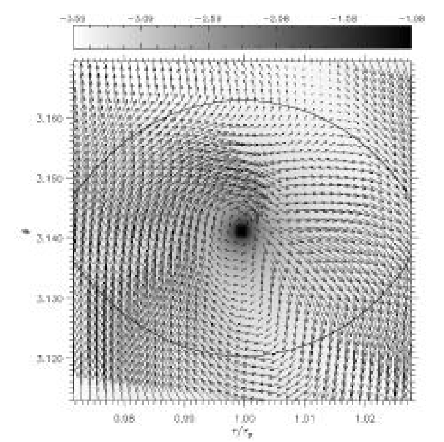
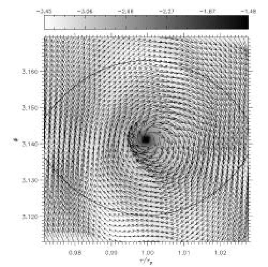
Figure 22: Density distribution and velocity field around $\mbox{$M_{\mathrm{p}}$}=1\;\mbox{$M_{\mathrm{J}}$}$ (top) and $\mbox{$M_{\mathrm{p}}$}=0.1\;\mbox{$M_{\mathrm{J}}$}$ (bottom) non-accreting models. Left panels show H-models while right ones show to C-models. Colors scale logarithmically in all of the panels. In the units used in the color bar, $-3$ corresponds to $\Sigma=328.7\;\mbox{$\mathrm{g}\,\mathrm{cm}^{\mathrm{-2}}$}$.

Accreting models assume that the planetary accretion rate can adjust to the rate at which matter can be supplied by the surrounding environment. We now investigate the opposite situation, namely when no further accretion onto the protoplanet is allowed.

The overall flow structure and density distribution of non-accreting protoplanets are drastically different from those of accreting ones. This can be clearly seen in Figure 22, where we show the surface density and the flow field for $\mbox{$M_{\mathrm{p}}$}=1\;\mbox{$M_{\mathrm{J}}$}$ (upper panels) and $0.1\;\mbox{$M_{\mathrm{J}}$}$ (lower panels) objects. The standard scenario of a Keplerian-like sub-disk is completely altered. This is a consequence of the large pressure gradient, built up by the large density gradient, which allows matter to move on orbits not constrained by the centrifugal balance. Therefore, the two-arm spiral feature is replaced by a more complex system of multiple shock fronts across which material is first deflected toward the planet and then ejected outward, as also indicated by the sign of the in-fall velocity $w_{\mathrm{in}}$ within the region.

The flow strongly diverges in a zone that has a radius equal to $\approx 0.4\,R_{\mathrm{H}}$ in the upper-left panel (H-Jupiter model) and to $\approx 0.2\,R_{\mathrm{H}}$ in the upper-right panel (C-Jupiter model). The average surface density inside of $R_{\mathrm{H}}/3$ is between one and two and a half orders of magnitude larger than that measured in accreting models. The mass collected in $s\leq 0.8\;R_{\mathrm{H}}$ is $1.97\times 10^{-4}\;\mbox{$M_{\mathrm{J}}$}$ and $4.30\times 10^{-5}\;\mbox{$M_{\mathrm{J}}$}$ for the Jupiter-mass H-model and the C-model, respectively. The azimuthal average of the circumplanetary density, around Jupiter-size objects, can be approximated to $\langle\Sigma\rangle\simeq 1.2\times 10^{4}\,\left(0.1\,R_{\mathrm{H}}/s\right)^{2.8}\;\mbox{$\mathrm{g}\,\mathrm{cm}^{\mathrm{-2}}$}$ (H-model) and to $\langle\Sigma\rangle\simeq 1.5\times 10^{3}\,\left(0.1\,R_{\mathrm{H}}/s\right)^{2.7}\;\mbox{$\mathrm{g}\,\mathrm{cm}^{\mathrm{-2}}$}$ (C-model). The top panel of Figure 23 shows the averaged surface density profiles around $\mbox{$M_{\mathrm{p}}$}=1\;\mbox{$M_{\mathrm{J}}$}$ (left).

A major difference can be also observed in the sub-disk circulation of low-mass models (Fig. 22, lower panels). In fact, the fluid rotates in a clockwise direction. In general, the direction of rotation in sub-disks is determined by the balance among the Coriolis force, the pressure gradient, and the gravitational attraction by the planet. Basically, referring to the lower-right panel of Figure 22, the Coriolis force deflects fluid elements, orbiting at $r\lesssim r_{\mathrm{p}}$, rightward. Therefore, it forces matter to cross the gap and to reconnect to the other side, while still moving in a position upstream of the perturber body. In contrast, the term $-\mathrm{d}P/\mathrm{d}s$, supposedly positive, opposes to reconnection when fluid is upstream of the planet’s location but favors it when matter is downstream of the planet. The prograde rotation that has been encountered so far indicates that the Coriolis deflection overwhelms the pressure gradient. For this reason reconnection across the gap always occurs upstream of the planet. Evidently, in the low-mass models ($\mbox{$M_{\mathrm{p}}$}=33\;\mbox{$M_{\oplus}$}$) displayed in the bottom panels of Figure 22, the pressure gradient drives material, flowing from upstream, past the planet’s position and forces it to circulate clockwise around the perturber. Consequently, matter entering the Hill sphere has an angular momentum anti-parallel (in the planet’s frame) to that of the circumstellar disk. In the range from $0.1$ to $1\,R_{\mathrm{H}}$, the magnitude of the rotational velocity $|\langle w_{\mathrm{rot}}\rangle|$ increases roughly as $\sqrt{s}$. The behavior of $\langle\Sigma\rangle$ resembles that of a power-law, as in Jupiter-mass cases, with powers $0.9$ and $0.5$, respectively for the H- and C-model (Fig. 23, right panel). Interestingly, no large differences are seen in the two density profiles.

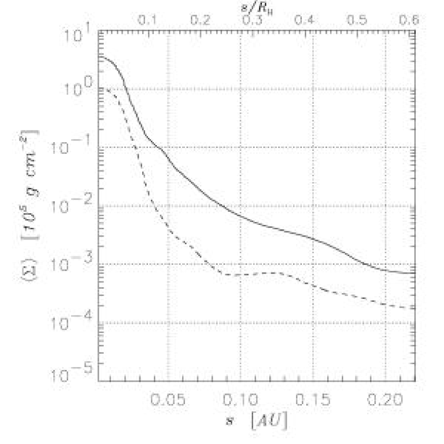
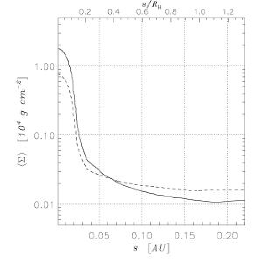
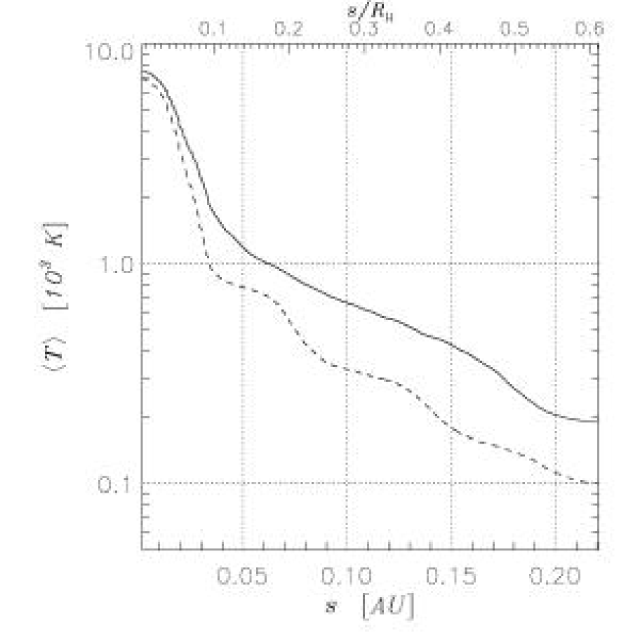
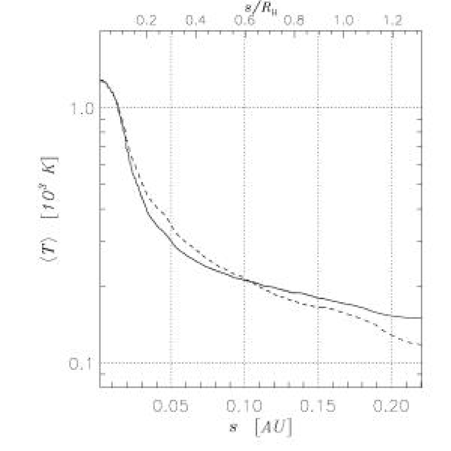
Figure 23: Average surface density (top) and temperature (bottom) around $1\;\mbox{$M_{\mathrm{J}}$}$ (left) and $0.1\;\mbox{$M_{\mathrm{J}}$}$ (right) non-accreting protoplanets. Solid lines refer to the H-models whereas short-dash and long-dash lines belong to C-models.

The high pressure gradient is also caused by the large temperature gradient. Parameters for analytic approximations of the average temperature $\langle T\rangle$, according to equation (38), are reported in Table 5.

Table 5: Fit Parameters for the Averaged Temperature Distribution: Non-Accreting Models.

	C-Models				H-Models
$\mbox{$M_{\mathrm{p}}$}/\mbox{$M_{\mathrm{J}}$}$	$\langle T\rangle_{\bar{s}}\;[\mbox{$\mathrm{K}$}]$	$\xi$	Range		$\langle T\rangle_{\bar{s}}\;[\mbox{$\mathrm{K}$}]$	$\xi$	Range
$1.0\phantom{0}$	$1.187\times 10^{3}$	$1.29$	$[0.05,1.0]\,R_{\mathrm{H}}$		$1.909\times 10^{3}$	$1.11$	$[0.05,1.0]\,R_{\mathrm{H}}$
$0.5\phantom{0}$	$1.132\times 10^{3}$	$0.81$	$[0.05,1.0]\,R_{\mathrm{H}}$		$1.458\times 10^{3}$	$1.00$	$[0.05,1.0]\,R_{\mathrm{H}}$
$0.2\phantom{0}$	$9.256\times 10^{2}$	$1.18$	$[0.05,1.0]\,R_{\mathrm{H}}$		$9.335\times 10^{2}$	$0.76$	$[0.05,1.0]\,R_{\mathrm{H}}$
$0.1\phantom{0}$	$7.570\times 10^{2}$	$0.70$	$[0.05,1.0]\,R_{\mathrm{H}}$		$6.242\times 10^{2}$	$0.59$	$[0.05,1.0]\,R_{\mathrm{H}}$
$0.06$	$6.103\times 10^{2}$	$0.60$	$[0.05,1.0]\,R_{\mathrm{H}}$

Note. — Parameters that enter equation (38) when applied to non-accreting models.

Maximum temperatures, at $s=0.1\,R_{\mathrm{H}}$, reach $1900\;\mbox{$\mathrm{K}$}$ and $1200\;\mbox{$\mathrm{K}$}$, in $\mbox{$M_{\mathrm{p}}$}=1\;\mbox{$M_{\mathrm{J}}$}$ H- and C-models respectively (bottom-left panel in Fig. 23). At the limit of the Roche lobe the temperature is somewhat higher than that measured in accreting models and depends on the gap structure. They vary from $\sim 100$ to $\sim 200\;\mbox{$\mathrm{K}$}$. Low mass models furnish temperatures that are very similar in both viscosity regimes.

It is worthy to notice that in either planetary-mass and viscosity case, the resulting temperature profiles are steeper than the ones shown in Figure 19 only when $s<0.1\,R_{\mathrm{H}}$, but they are nearly as steep past this distance. Actually, from Table 5 it appears the toward low planetary masses temperature profiles are even flatter. Performing the same check as done in the previous section, it turns out that $\left|\Lambda_{s}\right|/\left|\Lambda_{z}\right|$ is at most $0.3$. In fact, around Jupiter-mass planets, the ratio $H/s$ varies between $0.3$ and $0.5$, for distances larger than $0.1\,R_{\mathrm{H}}$. Hence, even in these circumstances the type of energy equation implemented here yields a reasonable description of the thermal structure of sub-disks, down to $\sim 0.1\,R_{\mathrm{H}}$.

7 Accretion and Migration

The evaluation of the mass accretion rate of protoplanets is carried out by reducing the surface density around the planet, according to a relation of the type $\Delta\Sigma/\Sigma=\Delta t/\tau_{\mathrm{ev}}$ (see, Paper I for details). This reduction process has a time scale $\tau_{\mathrm{ev}}$ that is much smaller than the integration time step $\Delta t$. In Figure 24 the planetary accretion rate $\dot{M}_{\mathrm{p}}$ evaluated in these computations is compared to that achieved with local-isothermal 2D (Paper I) and 3D (Paper II) models, where the disk mass was rescaled to match the values adopted here (see § 4).

In the context of the accretion history of protoplanets, it is worthwhile to stress that 2D calculations are only able to simulate the late stages of the accretion process, i.e., when it mainly occurs via mass transfer in the circumplanetary disk. This is consistent with the parameterization adopted here to describe the circumstellar environment.

Figure 24: Comparison of the accretion rates obtained from different types of simulations. Filled diamonds and squares indicate estimates provided by H- and C-models. Open triangles show data points from $\alpha$-viscosity models A2 (larger value) and A3. Asterisks and crosses represent the rates furnished by local isothermal computations in two (Paper I) and three (Paper II) dimensions, respectively. These last two sets of values are rescaled to match the disk mass $\mbox{$M_{\mathrm{D}}$}=4.8\times 10^{-3}\;\mbox{$M_{*}$}$, used in these simulations.

From Figure 24, one can see that C-models (filled squares) provide accretion rates quite similar to those obtained from models with a fixed temperature distribution (crosses). This occurrence is related to the quasi-Keplerian, circumplanetary flow observed in both kinds of computations. Jupiter-mass models with an $\alpha$-type viscosity (open triangles) give rates which are similar to that of the C-model when $\alpha=10^{-2}$ but somewhat lower ($\dot{M}_{\mathrm{p}}=6\times 10^{-3}\;\mbox{$M_{\oplus}$}\,\mathrm{yr}^{-1}$) when $\alpha=10^{-3}$, consistently with the low sub-disk mass measured in this case. H-models provide values of $\dot{M}_{\mathrm{p}}$ (filled diamonds) that, in case of Jupiter-size planets, fall above the estimates from all of the other models. According to the accretion procedure, the larger the amount of matter contained in the accretion region $s=\kappa_{\mathrm{ac}}$, the larger the accreted mass is. Within $s=0.1\,R_{\mathrm{H}}$ of a Jupiter-mass planet, the mean density computed in the H-model is roughly three times larger than that in the C-model (Fig. 14). This is related to the background gap density that is much higher in H-models, as reported in Table 2 (see also Fig. 7), due to the larger fluid viscosity.

Figure 25: Migration time scales plotted against the planetary mass. Notations are the same as in Figure 24. Data points indicate the magnitude of the total gravitational torque when this is computed excluding the contributions of matter residing inside of the sphere $s=R_{\mathrm{H}}$. Only accreting models are considered. As for $\alpha$-viscosity models (open triangles), A2 gives the faster migration rate of the two.

Figure 25 shows the total gravitational torque $\mathcal{T}_{\mathrm{D}}$ exerted by disk material onto accreting planets, as the inverse of the migration time scale ($\mathcal{T}_{\mathrm{D}}\propto|\dot{r}_{\mathrm{p}}|/r_{\mathrm{p}}\equiv 1/\tau_{\mathrm{M}}$). This quantity is computed from the gravitational force acting on the planet, as explained in Paper I. The length $\beta$ represents the radius of the circular region around the planet’s position whose contribution is not taken into account. In Figure 25, this length is set equal to $R_{\mathrm{H}}$. Outcomes from C-models, and generally those from H-models, compare well to the local-isothermal computations. Models with $\alpha$-viscosity provide migration rates on the same magnitude as well. C-models show a rather constant value of $\tau_{\mathrm{M}}$ as a function of the planet’s mass, whereas H-models present a minimum at $\mbox{$M_{\mathrm{p}}$}=0.2\;\mbox{$M_{\mathrm{J}}$}$. Migration time scales of H-models differ by less than a factor two from those of C-models. Only for $\mbox{$M_{\mathrm{p}}$}=33\;\mbox{$M_{\oplus}$}$, $\tau_{\mathrm{M}}$ is appreciably longer. One may attribute this effect to the absence of a real gap in this model (see Table 2), and thus to an early onset of the Type I drifting regime.

Table 6: Torques From Different Disk Regions: Accreting Models.

	Normalized Torques
Model	$\mathcal{A}$	$\mathcal{B}$	$\mathcal{C}$	$\mathcal{D}$
$1.0\;\mbox{$M_{\mathrm{J}}$}$ C	$0.0987$	$-1.9416$	$1.3707$	$-0.5278$
$1.0\;\mbox{$M_{\mathrm{J}}$}$ H	$0.3247$	$-13.538$	$12.828$	$-0.6147$
$1.0\;\mbox{$M_{\mathrm{J}}$}$ A3	$0.9857$	$-4.7780$	$4.9240$	$-2.1317$
$1.0\;\mbox{$M_{\mathrm{J}}$}$ A2	$0.0913$	$-2.1357$	$1.3905$	$-0.3461$
$0.5\;\mbox{$M_{\mathrm{J}}$}$ C	$0.1962$	$-3.6112$	$2.9099$	$-0.4949$
$0.5\;\mbox{$M_{\mathrm{J}}$}$ H	$0.3301$	$-14.940$	$14.084$	$-0.4732$
$0.2\;\mbox{$M_{\mathrm{J}}$}$ C	$0.4280$	$-13.852$	$13.176$	$-0.7520$
$0.2\;\mbox{$M_{\mathrm{J}}$}$ H	$0.2406$	$-14.827$	$13.840$	$-0.2536$
$0.1\;\mbox{$M_{\mathrm{J}}$}$ C	$0.4070$	$-17.989$	$17.211$	$-0.6290$
$0.1\;\mbox{$M_{\mathrm{J}}$}$ H	$0.6315$	$-36.823$	$35.768$	$-0.5765$
$20\;\mbox{$M_{\oplus}$}$ C	$0.3471$	$-17.656$	$16.800$	$-0.4911$

Note. — Gravitational torques exerted by the inner disk ($\mathcal{A}$) $r\leq r_{\mathrm{p}}-2.5\,R_{\mathrm{H}}$, and the outer disk ($\mathcal{D}$) $r\geq r_{\mathrm{p}}+2.5\,R_{\mathrm{H}}$. The remaining domain ($r_{\mathrm{p}}-2.5\,R_{\mathrm{H}}<r<r_{\mathrm{p}}+2.5\,R_{\mathrm{H}}$) is further divided in the trailing gap region ($\mathcal{B}$) $\varphi\leq\varphi_{\mathrm{p}}$, and the leading gap region ($\mathcal{C}$) $\varphi>\varphi_{\mathrm{p}}$. The width of the gap region is chosen according to the average width observed in Figure 7. All torques are normalized to the absolute value of the total torque $\mathcal{T}_{\mathrm{D}}$. Furthermore, they exclude the contribution from a circle of radius $R_{\mathrm{H}}$ centered on the planet.

In Table 6, we separate the contributions of different disk regions to the total torque $\mathcal{T}_{\mathrm{D}}$, introducing the inner disk ($\mathcal{A}$), the outer disk ($\mathcal{D}$) and the gap region ($\mathcal{B}$ and $\mathcal{C}$). Further details on the regions are reported in the Table’s note. All contributions are normalized to $|\mathcal{T}_{\mathrm{D}}|$. The width of the gap region is fixed to $5\,R_{\mathrm{H}}$ (see Fig. 7) and the zone behind the planet ($\mathcal{B}$) is distinguished from the one ahead of it ($\mathcal{C}$). Torques exerted from inside the Hill sphere are not accounted for. A large fraction of the contributions arising from zones $\mathcal{B}$ and $\mathcal{C}$ is actually generated in the coorbital regions, within a few Hill radii from the planet. From the entries in Table 6 one can argue that coorbital torques in H-models are larger in magnitude than they are in C-models. This is a consequence of the shallower gap of H-models. The situation is reversed in the $\alpha$-viscosity models because of the density humps at L4 and L5 Lagrangian points.

As for the influence of the parameter $\beta$ on the total torque, it turns out that H-models are generally more sensitive than C-models. By examining the function $\mathcal{T}_{\mathrm{D}}=\mathcal{T}_{\mathrm{D}}(\beta)$, some more insight can be gained. For $\mbox{$M_{\mathrm{p}}$}=1\;\mbox{$M_{\mathrm{J}}$}$ models (Fig. 26, top-left panel), no significant net torque arises from within the Hill sphere in the C-model (dashed line). The situation appears to be different for the H-model (solid line) because $\mathcal{T}_{\mathrm{D}}$ decreases to a minimum, around $\beta=R_{\mathrm{H}}/2$, and then increases and changes sign around $\beta=0.1\,R_{\mathrm{H}}$. Jupiter-mass $\alpha$-viscosity models (Fig. 26, top-right panel) display a smooth behavior since the total torque is rather constant down to $\beta=R_{\mathrm{H}}/2$. When $\beta$ diminishes, $\mathcal{T}_{\mathrm{D}}$ increases (i.e., it has smaller absolute values) and the model with $\alpha=10^{-3}$ (dashed line) shows a change of sign at $\beta=0.4\,R_{\mathrm{H}}$. When $\mbox{$M_{\mathrm{p}}$}=0.1\;\mbox{$M_{\mathrm{J}}$}$ (Fig. 26, bottom-left panel), in either case, $\mathrm{d}\mathcal{T}_{\mathrm{D}}/\mathrm{d}\beta<0$, because of the positive torques arising within the sub-disk. The rate of change is more drastic in the H-model, where the total torque becomes positive and keeps increasing when $\beta\lesssim R_{\mathrm{H}}/2$. Torques acting on the $20\;\mbox{$M_{\oplus}$}$ planet (Fig. 26, bottom-right panel) are strongly dependent on $\beta$, as positive torques are exerted down to $\approx 0.4\,R_{\mathrm{H}}$ and large negative torques arise between $\approx 0.2\,R_{\mathrm{H}}$ and $\approx 0.4\,R_{\mathrm{H}}$.

Figure 26: Inverse of the migration time scale versus the radius $\beta$ of the region excluded from the torque calculation. The quantity $v=\dot{a}/|\dot{a}|$ indicates the direction of the planet migration. Solid lines refer to models H or A2 while dashed lines refer models C or A3. Top-left panel. Jupiter-mass models H and C. Top-right. Jupiter-mass models with $\alpha$-viscosity A2 and A3. Bottom-left. $\mbox{$M_{\mathrm{p}}$}=0.1\;\mbox{$M_{\mathrm{J}}$}$ model H and C. Bottom-right. $\mbox{$M_{\mathrm{p}}$}=20\;\mbox{$M_{\oplus}$}$ C-model.

8 Conclusions

In this paper we presented two-dimensional simulations of disk-planet interactions in which we considered the joint thermo-hydrodynamics evolution of the system. In order to do that, we solved an energy equation that accounts for the major processes responsible for the energetic balance of fluid parcels. We restricted the treatment of the problem to a flat geometry in order to make some simplifying assumptions on the radiative part of the energy budget, i.e., to treat the radiation transfer as a cooling term. A nested-grid technique was used to resolve different length scales, therefore both the global and local features could be investigated.

The two-dimensional approximation has been proved to work reasonably well as long as the planetary mass is larger than a tenth of the mass of Jupiter (Paper II). Because of this, only planets more massive than $\approx 0.1\;\mbox{$M_{\mathrm{p}}$}$ have been simulated. In order to compromise with the lingering uncertainty on the viscosity magnitude and to inquire into different temperature regimes, we considered different constant viscosity and $\alpha$-viscosity models. Both accreting and non-accreting planets were simulated.

From the global point of view, and roughly speaking, we can conclude that circumstellar disk models with a fixed temperature distribution provide a reasonably good description of the system, though details of the gap structure and shape of the disk spirals differ. Around Jupiter-mass protoplanets, only with kinematic viscosities as low as $10^{15}\;\mbox{$\mathrm{cm}^{\mathrm{2}}\,\mathrm{s}^{\mathrm{-1}}$}$, a wide and deep gap is carved in whereas it reduces to a shallow density trough when the viscosity is ten times as large. Mean temperatures in the gap can be as low as $20$–$50\;\mbox{$\mathrm{K}$}$, depending on the viscosity regime. The most diluted and cold gap material is located where the circumplanetary disk merges into the gap. The aspect ratio appears smaller than $0.04$ and it is also marked by a gap-like feature, which shades the protoplanet’s environment against stellar radiation. The models with $\alpha=10^{-3}$ show a ring of matter within the gap that evolves on a viscous time scale. Regarding smaller planetary masses ($\mbox{$M_{\mathrm{p}}$}\approx 0.1\;\mbox{$M_{\mathrm{J}}$}$), both gap and spiral perturbations become quite faint features. Likely, only Jupiter-size bodies are capable of digging gaps deep enough to be observed by present-day instrumentation.

From the local point of view, we obtained the distribution of density, temperature, and other thermodynamical quantities in circumplanetary disks. Except for the $\alpha$-viscosity model with $\alpha=10^{-3}$, rather comparable outcomes are provided by models with different viscosity regimes. The density, averaged around the planet, shows an exponential radial decline. Sub-disks have masses on the order of $10^{-5}$–$10^{-6}\;\mbox{$M_{\mathrm{J}}$}$, which makes them gravitationally stable. Temperatures range from several hundred Kelvin degrees, at distances $s\lesssim 0.1R_{\mathrm{H}}$ from the planet, to values between $50$ and $100\;\mbox{$\mathrm{K}$}$, at the border of the Hill sphere. Azimuthal averages yield profiles dropping nearly as the inverse of the distance from the planet. Circumplanetary disks have aspect ratios $H/s$ around a few tenths and they tend to be optically thick. All of these properties appear to be consistent with the “fast-inflow” analytical models of protojovian disks recently developed by Canup & Ward (2002). By means of a semi-analytical treatment, we showed that, also in the sub-disk, the neglect of radial radiation transfer should not crucially affect our results. Non-accreting models furnish a rather different scenario. Around Jupiter-mass objects, circulation in the Roche lobe is not Keplerian-like because of the large pressure built up mainly by the density gradient and partly by the temperature gradient. Around $\mbox{$M_{\mathrm{p}}$}=0.1\;\mbox{$M_{\mathrm{J}}$}$, clockwise rotation establishes as a result of the weakening of the Coriolis force with respect to the pressure gradient term.

Accretion and migration rates inferred by these simulations are comparable to those evaluated with previous purely hydrodynamical local-isothermal computations. An analysis of the zonal torques indicates that coorbital torques increase as viscosity increases. Moreover, negative coorbital torques, arising from material outside of the Roche lobe and lagging behind the planet, are generally larger than those from material ahead of the planet. We also found that, in the two-dimensional approximation, the material lying inside of the Roche lobe is able to exert strong gravitational torques on the planet. Since the density gap is usually filled in H-models (see Table 2), Type I migration regime might extend to larger planetary masses (see Fig. 25).

In order to address the issue of how the third dimension affects the thermo-hydrodynamics of the system, both globally and locally around protoplanets, we are extending this study to 3D simulations in which radiation transfer is treated in the flux-limited diffusion approximation (Levermore & Pomraning, 1981).

References

- Agol et al. (2001) Agol, E., Krolik, J., Turner, N. J., & Stone, J. M. 2001, ApJ, 558, 543
- Alexander, Augason, & Johnson (1989) Alexander, D. R., Augason, G. C., & Johnson, H. R. 1989, ApJ, 345, 1014
- Armitage, Clarke, & Tout (1999) Armitage, P. J., Clarke, C. J., & Tout, C. A. 1999, MNRAS, 304, 425
- Bate et al. (2003) Bate, M. R., Lubow, S. H., Ogilvie, G. I., Miller K. A. 2003, MNRAS, 341,, 213
- Bell et al. (1997) Bell, K. R., Cassen, P. M., Klahr, H. H., & Henning, Th. 1997, ApJ, 486, 372
- Bell & Lin (1994) Bell, K. R. & Lin, D. N. C. 1994, ApJ, 427, 987
- Bryden et al. (1999) Bryden, G., Chen, X., Lin, D. N. C., Nelson, R. P., & Papaloizou, J. C. B. 1999, ApJ, 514, 344
- Calvet et al. (2002) Calvet, N., D’Alessio, P., Hartmann, L., et al. 2002, ApJ, 568, 1008
- Canup & Ward (2002) Canup, R. M., Ward, W. R. 2002, AJ, 124, 3404
- Collins, Helfer, & van Horn (1998) Collins, T. J. B., Helfer, H. L., & van Horn, H. M. 1998, ApJ, 502, 730
- Coradini et al. (1989) Coradini, A., Cerroni, P., Magni, G., & Federico, C. 1989, in Origin and Evolution of Planetary and Satellite Atmospheres, 723–762
- D’Alessio et al. (1998) D’Alessio, P., Canto, J., Calvet, N., & Lizano, S. 1998, ApJ, 500, 411
- D’Angelo, Henning, & Kley (2002) D’Angelo, G., Henning, Th., & Kley, W. 2002, A&A, 385, 647 (Paper I)
- D’Angelo, Kley, & Henning (2003) D’Angelo, G., Kley, W., & Henning, Th. 2003, ApJ, 586, 540 (Paper II)
- Dullemond et al. (2002) Dullemond, C. P., van Zadelhoff, G. J., & Natta, A. 2002, A&A, 389, 464
- Frank, King, & Raine (1992) Frank, J., King, A., & Raine, D. Accretion Power in Astrophysics, Cambridge University Press, 1992
- Godon (1996) Godon, P. 1996, ApJ, 463, 674
- Henning & Stognienko (1996) Henning, Th. & Stognienko, R. 1996, A&A, 311, 291
- Hubeny (1990) Hubeny, I. 1990, ApJ, 351, 632
- Huré et al. (2001) Huré, J.-M., Richard, D., & Zahn, J.-P. 2001, A&A, 367, 1087
- Klahr et al. (1999) Klahr, H. H., Henning, Th., & Kley, W. 1999, ApJ, 514, 325
- Kley (1999) Kley, W. 1999, MNRAS, 303, 696
- Kley, D’Angelo, & Henning (2001) Kley, W., D’Angelo, G., & Henning, Th. 2001, ApJ, 547, 457
- Levermore & Pomraning (1981) Levermore, C. D., Pomraning, G. C. 1981, ApJ, 248, 321
- Lin (1981) Lin, D. N. C. 1981, ApJ, 246, 972
- Lin & Papaloizou (1985) Lin, D. N. C. & Papaloizou, J. 1985, in Protostars and Planets II, 981–1072
- Lin & Papaloizou (1993) Lin, D. N. C. & Papaloizou, J. C. B. 1993, in Protostars and Planets III, 749–835
- Liu & Meyer-Hofmeister (1997) Liu, B. F. & Meyer-Hofmeister, E. 1997, A&A, 328, 243
- Lubow, Seibert, & Artymowicz (1999) Lubow, S. H., Seibert, M., & Artymowicz, P. 1999, ApJ, 526, 1001
- Lynden-Bell & Pringle (1974) Lynden-Bell, D. & Pringle, J. E. 1974, MNRAS, 168, 603
- Markwick et al. (2002) Markwick, A. J., Ilgner, M., Millar, T. J., & Henning, Th. 2002, A&A, 385, 632
- Masset (2002) Masset, F. S. 2002, A&A, 387, 605
- Matt et al. (2002) Matt, S., Goodson, A. P., Winglee, R. M., & Böhm, K. 2002, ApJ, 574, 232
- Mihalas & Weibel Mihalas (1999) Mihalas, D. & Weibel Mihalas, B. Foundations of radiation hydrodynamics, New York: Dover, 1999
- Miki (1982) Miki, S. 1982, Progress of Theoretical Physics, 67, 1053
- Miyoshi et al. (1999) Miyoshi, K., Takeuchi, T., Tanaka, H., & Ida, S. 1999, ApJ, 516, 451
- Morfill, Tscharnuter, & Voelk (1985) Morfill, G. E., Tscharnuter, W., & Voelk, H. J. 1985, in Protostars and Planets II, 493–533
- Morohoshi & Tanaka (2003) Morohoshi, K., Tanaka, H. 2003, MNRAS, submitted
- Nelson & Benz (2003a) Nelson, A., Benz, W. 2003, ApJ, 589, 556
- Nelson & Benz (2003b) Nelson, A., Benz, W. 2003, ApJ, 589, 578
- Nelson & Papaloizou (2003) Nelson, R. P., Papaloizou, J. C. B. 2003, MNRAS, 339, 993
- Nelson et al. (2000) Nelson, R. P., Papaloizou, J. C. B., Masset, F., & Kley, W. 2000, MNRAS, 318, 18
- Nomura (2002) Nomura, H. 2002, ApJ, 567, 587
- Papaloizou & Nelson (2003) Papaloizou, J. C. B., Nelson, R. P. 2003, MNRAS, 339, 983
- Papaloizou & Terquem (1999) Papaloizou, J. C. B. & Terquem, C. 1999, ApJ, 521, 823
- Popham et al. (1993) Popham, R., Narayan, R., Hartmann, L., & Kenyon, S. 1993, ApJ, 415, L127
- Pringle (1981) Pringle, J. E. 1981, ARA&A, 19, 137
- Rice et al. (2003) Rice, W. K. M., Kenneth, W., Armitage, P. J., Whitney, B. A., & Bjorkman, J. E. 2003, MNRAS, 342, 79
- Shakura & Sunyaev (1973) Shakura, N. I., Sunyaev R. A. 1973, A&A, 24, 337
- Steinacker & Henning (2003) Steinacker, J., Henning, Th. 2003, ApJ, 583, L35
- Stone & Norman (1992) Stone, J. M. & Norman, M. L. 1992, ApJS, 80, 753
- Suttner & Yorke (2001) Suttner, G. & Yorke, H. W. 2001, ApJ, 551, 461
- Tanaka, Takeuchi, & Ward (2002) Tanaka, H., Takeuchi, T., & Ward, W. 2002, ApJ, 565, 1257
- Tanigawa & Watanabe (2002) Tanigawa, T. & Watanabe, S. 2002, ApJ, 580, 506
- Winkler & Norman (1986) Winkler, K. A. & Norman, M. L., eds. 1986, Astrophysical Radiation Hydrodynamics
- Winters, Balbus, & Hawley (2003) Winters, W. F., Balbus, S. A., Hawley, J. F. 2003, ApJ, 589, 543
- Wolf et al. (2002) Wolf, S., Gueth, F., Henning, Th., & Kley, W. 2002, ApJ, 566, L97
- Ziegler (1998) Ziegler, U. 1998, Computer Physics Communications, 109, 111