Altered Luminosity Functions of Relativistically Beamed Jet Populations

Abstract

The intrinsic luminosity functions of extremely fast jets found in many active galaxies and gamma-ray bursts are difficult to measure since their apparent luminosities are strongly affected by relativistic beaming. Past studies have only provided analytical predictions for the beamed characteristics of populations in which all jets have the same Lorentz factor. However, the jets found in active galaxies are known to span a large range of speeds. Here we derive analytical expressions for the expected Doppler factor distributions and apparent (beamed) luminosity functions of randomly-oriented, two-sided jet populations which have bulk Lorentz factors distributed according to a simple power-law over a range [G1, G2]. We find that if a jet population has a uniform or inverted Lorentz factor distribution, its Doppler factor distribution and beamed luminosity function will be very similar to that of a jet population with Lorentz factors all equal to G2. In particular, the beamed and intrinsic luminosity functions will have the same slope at high luminosities. In the case of a steeply declining Lorentz factor distribution, the slopes at high luminosities will also be identical, but only up to an apparent luminosity equivalent to the upper cutoff of the intrinsic luminosity function. Also, at very high apparent luminosities, the slope will be proportional to the power law slope of the Lorentz factor distribution. At very low luminosities, the form of the apparent luminosity function is very sensitive to the lower cutoff and steepness of the Lorentz factor distribution. We discuss how it should be possible to recover useful information about the intrinsic luminosity functions of relativistic jets by studying flux-limited samples selected on the basis of beamed jet emission.

1 INTRODUCTION

The observed fluxes of highly relativistic jets such as those found in active galactic nuclei and gamma-ray bursts are subject to strong relativistic aberration and Doppler beaming effects. This poses a serious challenge for determining the intrinsic luminosity functions (LFs) of these objects. Previous studies (e.g., Jackson & Wall 1999; Urry & Shafer 1984; Urry & Padovani 1991; Urry et al. 1991; Urry & Padovani 1995) have discussed in detail how luminosity functions can be apparently altered by Doppler beaming, but present analytical expressions only for cases where every jet in the population has the same intrinsic jet speed. In their analysis of beamed luminosity functions, Urry et al. (1991) found evidence that BL Lac objects could be the beamed counterparts of FR-I galaxies, provided that they have a wide distribution of jet Lorentz factors. Large proper motion surveys (Vermeulen et al., 2003; Kellermann et al., 2003) have also revealed that the overall AGN population contains a wide range of apparent jet speeds, which is inconsistent with a single-valued intrinsic speed distribution (Vermeulen & Cohen, 1994; Lister & Marscher, 1997).

Here we extend the earlier work of Urry & Padovani (1991) by deriving full analytical expressions for the Doppler factor distributions and beamed luminosity functions of randomly-oriented, two-sided jet populations that contain a range of jet speed $v$. We use an improved method that involves first deriving the predicted Doppler factor distribution, and then integrating over an appropriate range of Doppler factor to obtain the apparent luminosity function. We show how this method results in a much wider number of scenarios that can be treated fully analytically.

For simplicity, we consider only straight jets, where the emission is beamed proportionally according to the Lorentz factor of the jet flow (defined as $\gamma=(1-(v/c)^{2})^{-1/2}$, where $c$ is the speed of light). We restrict our analysis to cases where the jet Lorentz factors are distributed according to a power law, since this distribution provides the best fit to the apparent speed distribution of AGN jets (Lister & Marscher, 1997). Other forms, such as Gaussian and single-valued functions, provide very poor fits to the observed speeds.

In § 2 we outline our model assumptions and derive the predicted Doppler factor distributions for Lorentz factor distributions of the form $P_{\gamma}\propto\gamma^{a}$. We use these results in § 3 to examine how a simple intrinsic power-law luminosity function $\phi({\cal L})\propto{\cal L}^{-B}$ is transformed by Doppler boosting into its observed form $\Phi(L)$. In § 4 we discuss how our results can be applied to recover useful information about the parent population of samples dominated by relativistic jet emission, such as gamma-ray bursts, gamma-ray loud AGN, and core-dominated, radio-loud AGN. We summarize our findings in § 5.

2 DOPPLER BEAMING FACTOR DISTRIBUTIONS

For the purposes of obtaining analytical expressions, we adopt a simple model in which each source in the population contains two identical, straight, oppositely-directed jets with bulk Lorentz factor $\gamma$. We assume that the jet axes are randomly oriented, so that if $\theta$ represents the angle between the jet axis and the line of sight, then $P_{\theta}=\sin{\theta}$, and $0\arcdeg\leq\theta\leq 90\arcdeg$, where $P_{\theta}$ represents the probability density function of the viewing angles. The Lorentz factors have a density function $P_{\gamma}$ that is positive and non-zero over the region $\gamma_{1}\leq\gamma\leq\gamma_{2}$. The kinematic Doppler factor is defined as

$$\delta=\left[\gamma-\sqrt{\gamma^{2}-1}\cos{\theta}\right]^{-1},$$ (1)

and represents the frequency shift between the observer and jet rest frames. The minimum possible Doppler factor is $\delta_{min}=\gamma_{2}^{-1}$, and occurs when $\theta=90\arcdeg$. The maximum possible Doppler factor in the population is $\delta_{max}=\gamma_{2}(1+\beta_{2})$, where $\beta=v/c$, and occurs when $\theta=0\arcdeg$. When $\gamma_{2}$ is large, $\delta_{max}\simeq 2\gamma_{2}$.

In Appendix A we derive the expected Doppler factor distributions of randomly-oriented jet populations having various Lorentz factor distributions. We plot some individual cases corresponding to single-valued and power-law distributions in Figure 1.

2.1 Single-Valued Lorentz Factor Distributions

The two thick lines in Figure 1 represent populations where all jets have the same intrinsic Lorentz factor $\gamma_{o}$, with the dotted-dashed line corresponding to $\gamma_{o}=3$, and the solid line corresponding to $\gamma_{o}=30$. The latter represents the fastest jet speed typically seen in large AGN proper-motion surveys (Kellermann et al., in preparation). For a single-valued Lorentz factor distribution, $P_{\delta}\propto\delta^{-2}$, which corresponds to a straight line with slope of $-2$ in our log-log plot (Fig. 1).

2.2 Power-Law Lorentz Factor Distributions

The thin curves in Figure 1 correspond to various jet populations with Lorentz factors distributed between $1\leq\gamma\leq 30$. The thin dotted-dashed line shows the expected Doppler factor distribution for a jet population with an inverted $\gamma$ distribution (i.e., $P_{\gamma}\propto\gamma$). The thin dashed curve represents a uniform $\gamma$ distribution ($P_{\gamma}=$ constant). These two curves have an overall slope that is roughly the same as in the single-valued case (slope = $-2$) over a wide range of $\delta$, but they both taper off sharply near $\delta_{min}$ and $\delta_{max}$. Jets with these extreme Doppler factors all have Lorentz factors $\simeq\gamma_{2}$, and viewing angles close to $90\arcdeg$ and $0\arcdeg$, respectively. They are therefore very rare in the population. In the case of models where $P_{\gamma}\propto\gamma^{a}$ and $a\leq 0$, the tapering off at the extrema is a result of having relatively fewer jets with $\gamma=\gamma_{2}$, as compared to a single-valued population where all the jets have the same jet speed.

The remaining two curves in Figure 1 represent the cases $P_{\gamma}\propto\gamma^{-1}$ (thin solid line) and $P_{\gamma}\propto\gamma^{-2}$ (thin dotted line). In populations such as these which have few high-speed jets, the distributions taper off much more sharply for Doppler factors above $\gamma_{1}^{-1}$.

The slopes of the $P_{\delta}$ functions have a discontinuity at $\delta=\gamma_{1}^{-1}$, which arises because, if $\gamma_{2}>\gamma_{1}(1+\beta_{1})$, potentially any jet in the population can have a Doppler factor in the range $\gamma_{1}^{-1}<\delta<\gamma_{1}(1+\beta_{1})$. This leads to a slight over-density of sources in this interval. For a jet to have a Doppler factor that lies outside this range, it must have a speed greater than (but not equal to) $\beta_{1}$.

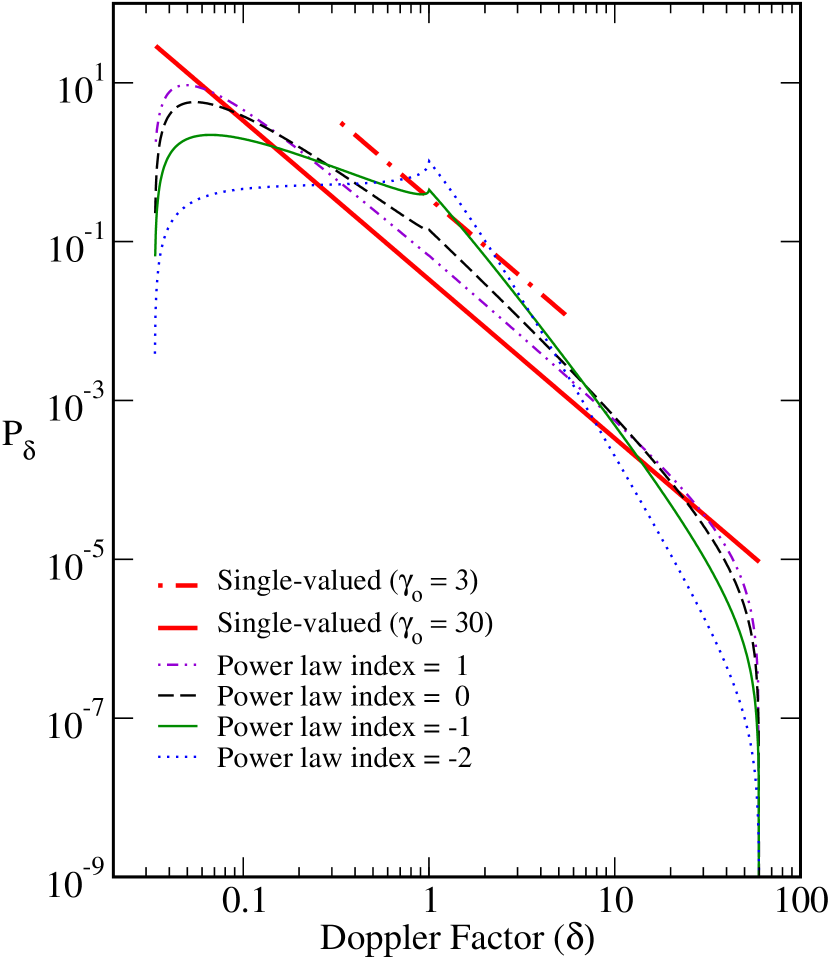
Figure 1: Predicted Doppler boosting factor distribution functions for randomly-oriented populations of two-sided jets. The thick dot-dashed and dotted lines correspond to a jet population having a single bulk Lorentz factor of $\gamma_{o}=3$ and $\gamma_{o}=30$, respectively. The thin lines correspond to jet populations whose bulk Lorentz factors are distributed over the range $1\leq\gamma\leq 30$ with a density function $P_{\gamma}\propto\gamma^{a}$. The models plotted correspond to $a=1$ (thin dot-dashed line), $a=0$ (thin dashed line), $a=-1$ (thin solid line), and $a=-2$ (thin dotted line).

2.3 Discussion

We have shown that the power-law slope of the Lorentz factor distribution can have a strong influence on the distribution of Doppler factors in a randomly-oriented jet population. In Figure 2 we show the effects of increasing the lower limit of the Lorentz factor distribution on a population with $\gamma_{1}\leq\gamma\leq\gamma_{2}$ and $P_{\gamma}\propto\gamma^{-2}$. As $\gamma_{1}$ is increased, the region $\gamma_{1}^{-1}<\delta<\gamma_{1}(1+\beta_{1})$ grows wider, and the cusp at $\delta=\gamma_{1}^{-1}$ is replaced by a broad region with slope equal to $-2$. The same behavior also occurs for other values of $a$. Figure 2 also confirms that the Doppler factor distribution approaches that of the single-valued Lorentz factor case as $\gamma_{1}\rightarrow\gamma_{2}$.

It is important to note that in a sample of purely randomly-oriented two-sided jets, exactly half will have approaching jet viewing angles greater than $60\arcdeg$. This means that regardless of the form of the jet Lorentz factor distribution, there will always be a preponderance of sources with low Doppler factors, such that the mean value of $\delta$ will always be less than unity. Somewhat paradoxically, if a jet population is measured to have a high mean Doppler factor, this actually implies that it must be dominated by slow jets. We caution, however, that this reasoning only applies to genuinely orientation-unbiased samples. Flux-limited samples selected on the basis of relativistically-beamed jet emission, on the other hand, will be strongly biased toward small viewing angles, and as a result will always be dominated by intrinsically fast jets with high Doppler factors (i.e., blazars; see Vermeulen & Cohen 1994).

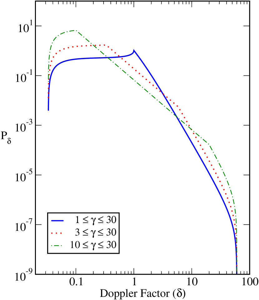
Figure 2: Predicted distribution functions of Doppler factor for jet populations with bulk Lorentz factors distributed according to $P_{\gamma}\propto\gamma^{-2}$, and ranging up to $\gamma_{2}=30$. The solid curve shows the predicted distribution for a lower limits of $\gamma_{1}=1$, while the dotted and dot-dashed curves represent models with $\gamma_{1}=3$ and $\gamma_{1}=10$, respectively.

3 BEAMED LUMINOSITY FUNCTIONS

We now use our results on the predicted Doppler factor distributions to derive the corresponding apparent luminosity functions of relativistically beamed jet populations. For the purposes of obtaining analytical expressions, we will ignore any luminosity contribution from the jet in each source that is pointing away from the observer. In § 3.1 we will show using numerical simulations that for a steep intrinsic LF, the receding (counter-jet) luminosity only affects the shape of the faint end of the beamed LF, and has no effect at high observed luminosities.

Due to relativistic aberration, the luminosity of an isotropically-emitting, moving object according to a stationary observer is

$$L=\delta^{p}{\cal L},$$ (2)

where ${\cal L}$ is the source rest-frame luminosity, $p=2-\alpha$ for continuous jet emission, and $\alpha$ is the spectral index ($S_{\nu}\propto\nu^{\alpha}$). In the case of a discrete emitting region, we have $p=3-\alpha$ due to relativistic time dilation of its finite synchrotron-emitting lifetime (Lind & Blandford, 1985). For fixed $p$, the observed luminosity function of a population of relativistic jets will depend solely on its Doppler factor distribution and its intrinsic (unbeamed) luminosity function. In the figures that follow, we will only plot models with $p=2$, which is appropriate for the continuous jet emission associated with the flat-spectrum cores of blazars.

We begin by assuming that the jet population has an intrinsic power-law luminosity function of the form:

$$\phi({\cal L})=\cases{k_{1}{\cal L}^{-B}&for ${\cal L}_{1}\leq{\cal L}\leq{\cal L}_{2}$\cr 0\;,&elsewhere,}$$ (3)

where the normalization constant is

$$k_{1}={1-B\over{\cal L}_{2}^{1-B}-{\cal L}_{1}^{1-B}}\;.$$ (4)

The transformation law for probability density functions yields the joint probability function

$$h(L,\delta)=P_{\delta}(\delta)\phi({\cal L}){d{\cal L}\over dL}.$$ (5)

Using equations (2) and (5) and the intrinsic luminosity function, we obtain

$$h(L,\delta)=k_{1}L^{-B}P_{\delta}(\delta)\;\delta^{-p(1-B)}.$$ (6)

Integrating over $\delta$ gives

$$\Phi(L)=k_{1}L^{-B}\int P_{\delta}(\delta)\;\delta^{Cp+1}d\delta,$$ (7)

where (using the notation of Urry & Shafer 1984)

$$C=B-(1/p)-1\;.$$ (8)

In their derivation of the beamed LF for a jet population having a unique Lorentz factor, Urry & Shafer (1984) identified several important values of L. Here we keep their definitions of $L_{3}$ and $L_{4}$, and extend their notation as follows:

$$L_{min}= {\cal L}_{1}\gamma_{2}^{-p}$$ (9)

$$L_{5}= {\cal L}_{1}\gamma_{1}^{-p}$$ (10)

$$L_{6}= {\cal L}_{1}(\gamma_{1}+\gamma_{1}\beta_{1})^{p}$$ (11)

$$L_{4}= {\cal L}_{1}\;\delta_{max}^{p}$$ (12)

$$L_{3}= {\cal L}_{2}\gamma_{2}^{-p}$$ (13)

$$L_{7}= {\cal L}_{2}\gamma_{1}^{-p}$$ (14)

$$L_{8}= {\cal L}_{2}(\gamma_{1}+\gamma_{1}\beta_{1})^{p}$$ (15)

$$L_{max}= {\cal L}_{2}\;\delta_{max}^{p}.$$ (16)

We note that a similar extension of notation was made by Urry & Padovani (1991), however, they do not include the parameter $L_{5}$, which is needed for the analytical solutions presented in Appendix B.

When $\gamma_{2}$ is large, the beamed LF spans a wide range:

$$L_{max}/L_{min}=\gamma_{2}^{2p}(1+\beta_{2})^{p}({\cal L}_{2}/{\cal L}_{1}).$$ (17)

Thus, even a jet population with a single intrinsic luminosity ${\cal L}={\cal L}_{1}={\cal L}_{2}$ will end up with a broad beamed luminosity function. This scenario has been invoked to explain the wide range of observed luminosities in gamma-ray bursts, which are thought to have Lorentz factors on the order of 100 (e.g., Kumar & Piran 2000).

To determine an analytical expression for the beamed LF, we substitute the relevant expression for $P_{\delta}$ (see eq. A9) into equation (7) and integrate over appropriate limits. We find that analytical solutions are generally only possible when the product $Cp$ is an integer. We derive expressions for several cases in Appendix B.  For simplicity, we have considered only cases where $B\geq(p+1)/p$ and $L_{3}>L_{4}$. This corresponds to the condition $({\cal L}_{2}/{\cal L}_{1})^{1/p}>\gamma_{2}^{2}(1+\beta_{2})$, which will always be satisfied provided ${\cal L}_{2}$ is made arbitrarily large. The latter can be justified if, as in our case, the intrinsic LF slope is fairly steep (i.e., $B\geq 1.5$ for $p=2$). With these choices of parameters, the $L$ values in equation (16) are arranged in order of increasing apparent luminosity.

In Figure 3 we plot $\log{\left[L\;\Phi(L)\right]}$ versus $\log{[L/{\cal L}_{1}]}$ for various power-law Lorentz factor distributions distributed over the range $1\leq\gamma\leq 30$. The thick solid curve is the original (unbeamed) LF, which in this example has a power-law slope equal to $-2$ and $\log{[{\cal L}_{2}/{\cal L}_{1}]}=7$. The remaining curves represent the beamed LFs for various values of power-law index $a$, where $P_{\gamma}\propto\gamma^{a}$.

Urry & Shafer (1984) found that for a single-valued Lorentz factor distribution, the beamed luminosity function will have the same slope as the unbeamed one for $L>L_{4}$, except in the immediate vicinity of $L_{max}$. In their numerical analysis, Urry & Padovani (1991) claimed that this also holds true for a distribution of Lorentz factors. We confirm this in the case of flat or inverted Lorentz factor distributions (i.e., $a=0$ and $a=1$). Indeed, the beamed LFs of a single-valued model with $\gamma=\gamma_{o}$ and a uniformly distributed model ($P_{\gamma}\propto\gamma\,;\;1\leq\gamma\leq\gamma_{o}$) are nearly identical for $L>L_{4}$ (see Fig. 4).

For steep power-law $\gamma$ distributions with $a\leq-1$, the beamed and unbeamed LFs also have the same slope, however, this is true only for the region $L_{4}<L<L_{8}$. Above $L_{8}$, the slope steepens by an amount proportional to the power-law $\gamma$ index $a$. We note that in the case of a jet population where ${\cal L}_{2}/{\cal L}_{1}$ is large and the intrinsic LF is steep, objects with $L>L_{8}$ will be extremely rare. In the models shown in Figure 3, only one jet in $~{}\sim 10^{7}$ will have $L>L_{8}$.

At luminosities fainter than $L_{4}$, Urry & Padovani (1991) claimed that the slope will always be equal to $-(p+1)/p$, regardless of the Lorentz factor distribution. However, we find this is true only in cases where there are very few low-Lorentz factor jets in the population (i.e., when $\gamma_{1}>>1$ or $a>0$). In cases where $\gamma_{1}\simeq 1$ and the Lorentz factor distribution is steep, the LF slope at low luminosities is significantly flatter than $-(p+1)/p$, and can even be highly inverted (see Fig 3). We caution, however, that at these low-luminosities many jets will lie in the plane of the sky, and that our analytical expressions ignore the receding jet. Adding the counterjet’s contribution to the total emission will change the predicted luminosity functions slightly. We discuss this issue in more detail in the next section.

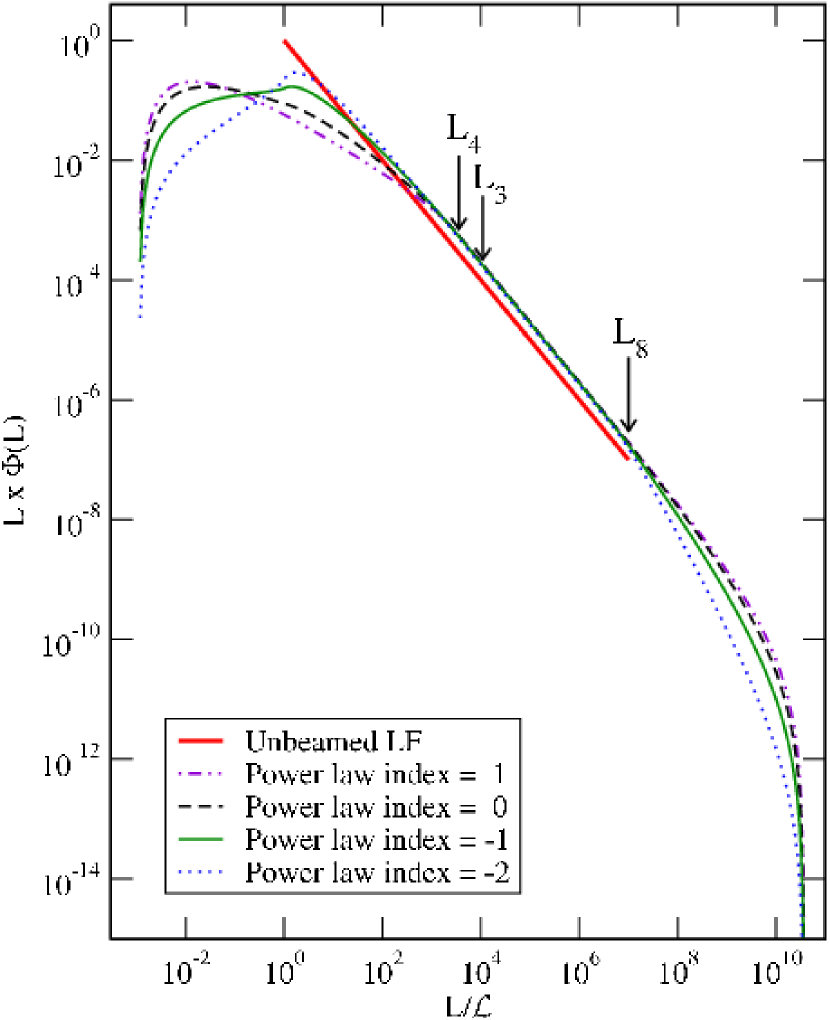
Figure 3: Predicted apparent luminosity functions (LFs) for jet populations with Lorentz factors distributed according to a simple power law. The intrinsic LF (thick solid curve) has a power-law slope of $-2$, and ranges from ${\cal L}_{1}$ to ${\cal L}_{2}$, with ${\cal L}_{2}/{\cal L}_{1}=10^{7}$. The remaining curves represent the beamed (apparent) LFs for jet populations with Lorenz factors distributed according to $P_{\gamma}\propto\gamma^{a}$ over the range $1\leq\gamma\leq 30$. These models plotted correspond to $a=1$ (thin solid curve), $a=0$ (dotted curve), $a=-1$ (dot-dashed curve), and $a=-2$ (dashed curve). The specific locations of $L_{3}$, $L_{4}$, and $L_{8}$ are marked with arrows (see eq. 16).

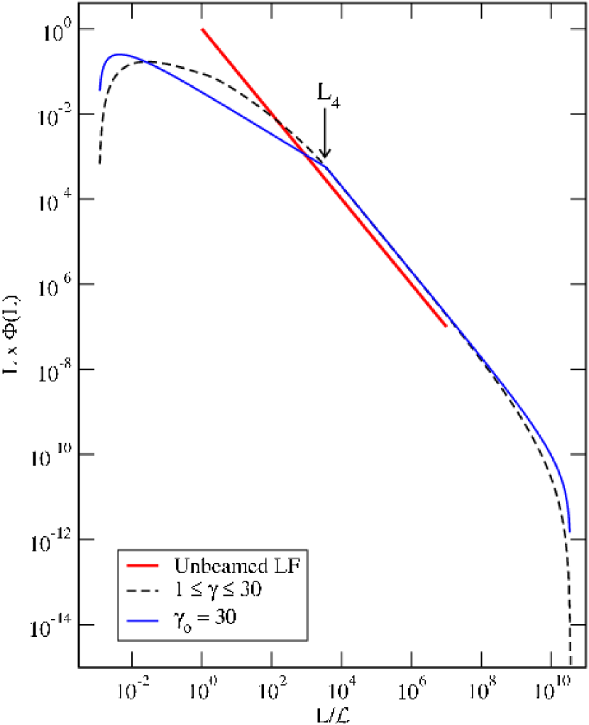
Figure 4: Comparison of beamed luminosity functions for jet populations with single-valued and power-law Lorentz factor distributions. The thick solid line represents the intrinsic LF, which has a power-law slope of $-2$, and ranges over ${\cal L}_{1}$ to ${\cal L}_{2}$, with ${\cal L}_{2}/{\cal L}_{1}=10^{7}$. The other curves represent beamed LFs for a jet population with a single Lorentz factor $\gamma_{o}=30$ (thin solid curve), one with Lorentz factors uniformly distributed over the range $1\leq\gamma\leq 30$ (dotted curve).

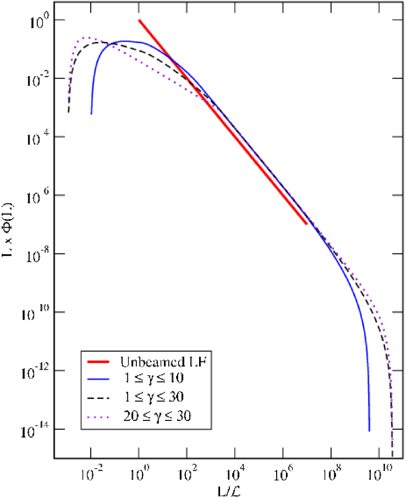
Figure 5: Comparison of beamed luminosity functions for jet populations with Lorentz factors uniformly distributed over different ranges (i.e., $P_{\gamma}\propto$ constant, where $\gamma_{1}\leq\gamma\leq\gamma_{2}$). The thick solid line represents the intrinsic LF, which has a power-law slope of $-2$, and ranges over ${\cal L}_{1}$ to ${\cal L}_{2}$, with ${\cal L}_{2}/{\cal L}_{1}=10^{7}$. The other curves represent the beamed LFs of jet populations with $1\leq\gamma\leq 10$ (thin solid curve), $1\leq\gamma\leq 30$ (dot-dashed curve), $20\leq\gamma\leq 30$ (dotted curve).

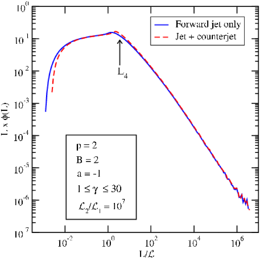
Figure 6: Beamed luminosity functions for two relativistic two-sided jet populations with identical Lorentz factor distributions and intrinsic luminosity functions. The dashed line is calculated numerically, and shows the beamed LF if the luminosity from both the approaching and receding jets in each source are considered. The solid line shows the expected LF if the receding jet is ignored. The two curves differ only at low apparent luminosities, where the Doppler factors are small and the approaching and receding jets have similar luminosities.

We have also investigated the effects of various ranges of Lorentz factor on the apparent luminosity functions of jet populations. In Figure 5 we plot three different models with Lorentz factors uniformly distributed over different ranges $\gamma_{1}\leq\gamma\leq\gamma_{2}$. It is apparent that for $L>L_{4}$, the bright end of the beamed LF is largely insensitive to the values of $\gamma_{1}$ and $\gamma_{2}$. Increasing $\gamma_{2}$ can potentially increase the number of ultra-high luminosity objects, but again these are likely to be extremely rare for steep intrinsic LFs.

At faint luminosities, the beamed LF is highly sensitive to the value of $\gamma_{2}$, since this dictates the minimum Doppler factor, and hence $L_{min}$. Because a very fast jet population will have a low mean Doppler factor (see § 2.3), its sources will, on average, appear fainter than those of a population dominated by slow speeds. Again, this reasoning applies only to genuinely orientation-unbiased samples.

3.1 Two-sided jets

The beamed luminosity functions presented in the previous section are not strictly correct at low luminosities, since they ignore any luminosity contribution from the receding jet in each source. When considering only highly beamed objects such as blazars or gamma-ray bursts, this is a reasonable approximation, since the receding jet will be extremely faint (and usually undetectable). However, in samples containing mildly relativistic jets, or jets that lie close to the plane of the sky (e.g., lobe-dominated radio galaxies), both the approaching and receding jets can contribute roughly equal amounts of flux.

In Figure 6 we compare two models with $B=2$, $a=-1$, $1\leq\gamma\leq 30$, and ${\cal L}_{2}/{\cal L}_{1}=10^{7}$. The solid line shows the beamed luminosity function if only the luminosity of the approaching jet is considered. The dashed line represents a numerically-determined beamed LF in which the luminosities of both the approaching and receding jets are taken into account. For luminosities below $L_{1}$, the curves differ considerably, since these jets lie close to the plane of the sky. At higher luminosities, the predicted LFs are virtually identical, since the apparent approaching/receding jet luminosity ratio becomes very large for small viewing angles and high Lorentz factors. We find that this result holds true for all ranges of $B$ and $a$ discussed in this paper. We conclude therefore, that the emission from the receding jet can be safely ignored when studying the luminosity functions of highly beamed objects.

4 OBSERVATIONAL IMPLICATIONS

The analytical results derived in this paper are applicable to any astronomical sample that is selected solely on the basis of relativistically-beamed jet emission. Our results are particularly relevant to compact radio-loud AGN, whose high-frequency radio emission originates primarily from milliarcsecond-scale relativistic jets. With the advent of dedicated VLBI arrays, it is now possible to conduct large multi-epoch surveys of these objects (e.g., the Caltech-Jodrell Surveys; Taylor et al. 1996 and the VLBA 2 cm Survey; Kellermann et al. 1998). However, because of the high thresholds required for fringe detection, these large VLBI studies have so far been confined to the brightest, most compact objects whose radiation is highly beamed toward us. These types of samples are not ideal for studying the general properties of the AGN jets, since one must first disentangle the combined effects of beaming, jet axis orientation bias, and Malmquist bias before one can construct a luminosity function or intrinsic speed distribution. Monte Carlo simulations have played an important role in this respect. Lister & Marscher (1997) showed that based on their observed superluminal speed distribution, AGN jets must have a wide range of Lorentz factors distributed according to a relatively steep power law ($P_{\gamma}\propto\gamma^{a}$, where $a\simeq-1.5$). They also demonstrated that a reasonably large, flux-limited sample of bright jets should always contain some objects with apparent speed equal to the maximum jet Lorentz factor in the parent population.

Since the observed LF of radio-loud AGN is fairly steep $(B\simeq 1.9\pm 0.1$; Willott et al. 1998), our findings suggest that the observed LF of a complete flux-limited sample selected on the basis of beamed emission will closely match the intrinsic LF for luminosities in the range $4{\cal L}_{1}\beta_{a,max}^{2}\mathrel{\hbox{\hbox to0.0pt{\hbox{\lower 4.0pt\hbox{$\sim$}}\hss}\hbox{$<$}}}L\mathrel{\hbox{\hbox to0.0pt{\hbox{\lower 4.0pt\hbox{$\sim$}}\hss}\hbox{$<$}}}{\cal L}_{2}$. Here we have assumed a boost index $p=2$ and $\gamma_{2}$ equal to the maximum apparent speed $\beta_{a,max}$. The lower luminosity limit ${\cal L}_{1}$ can be constrained using the nearest sources in a complete VLBI flux-limited sample, since these will generally meet the flux density criteria on the basis of their cosmological proximity, and not their Doppler boosting factors. The upper luminosity limit ${\cal L}_{2}$ can be constrained using the observed space density of radio-loud AGN.

We are currently gathering VLBI proper motion and flux density data at 15 GHz on a sample of the brightest $\sim 130$ jets in the northern sky. This sample, entitled MOJAVE (Monitoring Of Jets in AGN with VLBA Experiments; Zensus et al. 2003), is complete on the basis of compact (VLBI) flux density, and is therefore well-suited for exploring the intrinsic luminosity function of AGN jets. An analysis of the MOJAVE data is currently underway, and the results will be discussed in an upcoming paper.

5 SUMMARY

Astronomical samples of objects selected on the basis of emission from relativistic jets, such as gamma-ray bursters, gamma-ray loud AGN, and compact radio-loud AGN, will by highly affected by relativistic beaming effects. In particular, their observed luminosities are predicted to be enhanced by a factor $\delta^{p}$, where $\delta$ is the Doppler factor. We have derived expressions for the predicted Doppler factor distributions of two-sided, randomly-oriented, straight jet populations whose bulk Lorentz factors are distributed in the range $[\gamma_{1},\gamma_{2}]$ according to a simple power-law $P_{\gamma}\propto\gamma^{a}$. We summarize our findings as follows:

• The minimum and maximum jet Doppler factor in the population will depend only on the maximum Lorentz factor $\gamma_{2}$. Specifically, $\delta_{min}=\gamma_{2}^{-1}$, and $\delta_{max}=\gamma_{2}(1+\beta_{2})$.

• An orientation-unbiased sample of jets will always have a mean Doppler factor less than unity, since the majority of jets will lie close to the plane of the sky. Accordingly, a jet population weighted toward very fast speeds will have a lower mean Doppler factor, and therefore appear fainter than an identical jet population with slower intrinsic jet speeds.

• A randomly-oriented jet population with a flat ($a=0$) or inverted ($a=1$) Lorentz factor distribution will have a Doppler factor distribution very similar to a population where all jets have $\gamma=\gamma_{2}$. Over a broad range of $\delta$, the distribution function $P_{\delta}$ will vary as $\delta^{-2}$, except near $\delta_{min}$ and $\delta_{max}$, where much fewer sources are expected compared to the single-valued case. Sources with the highest possible Doppler factors near $\delta_{max}$ will always be rare, even when all the jets in the population are highly relativistic (i.e., $\gamma_{1}>>1$). This is a consequence of the extremely small angles to the line of sight that are necessary for high Doppler factors.

We have also derived analytical expressions for the apparent luminosity functions (LFs) of relativistic jet populations having a power-law distribution of Lorentz factors and a steep intrinsic power-law luminosity function. We find that:

• The slope of the apparent LF at low luminosities is not always equal $-(p+1)/p$, as claimed by Urry & Padovani (1991). The apparent LF in this region is highly sensitive to the speed distribution of the parent population. In particular, if the parent population is dominated by slow jets, the LF slope will be very flat or inverted at low luminosities.

• Regardless of the values of $\gamma_{1}$ and $\gamma_{2}$, when the Lorentz factor distribution of the jet population is steep (i.e., $a\leq-1$, where $P_{\gamma}\propto\gamma^{a}$), the intrinsic and beamed LFs will have the same slope over the range ${\cal L}_{1}\delta_{max}^{p}\leq L\leq{\cal L}_{2}$, where $L$ is the observed luminosity and ${\cal L}_{1}$ and ${\cal L}_{2}$ are the lower and upper cutoffs on the intrinsic LF, respectively.

• Since the intrinsic LF of radio-loud AGN jets is known to be steep, it should be possible to investigate its properties using flux-limited VLBI samples of highly beamed AGN jets. Such samples will have to be selected at relatively high radio frequencies (e.g. above $\sim 10$ GHz) in order to eliminate any contribution from un-beamed, steep-spectrum emission. An analysis of such a sample selected at 15 GHz (MOJAVE) is underway, and will be presented in an upcoming paper.

Appendix A DOPPLER FACTOR DISTRIBUTIONS OF JET POPULATIONS WITH A POWER LAW DISTRIBUTION OF LORENTZ FACTORS

We wish to determine the probability density function $P_{\delta}(\delta)$, which describes the expected distribution of Doppler factors for a randomly-oriented, two-sided jet population. The theory of probability transformation for several variables implies

$$g(\delta,\gamma)=P_{\gamma}(\gamma)P_{\theta}(\theta)\left|d\theta\over d\delta\right|.$$ (A1)

Now

$$\left|{d\delta\over d\theta}\right|=\delta^{2}\sqrt{\gamma^{2}-1}\;\sin{\theta}.$$ (A2)

Since the viewing angles are distributed according to

$$P_{\theta}(\theta)=\sin{\theta},$$ (A3)

we have

$$g(\delta,\gamma)={P_{\gamma}(\gamma)\over\delta^{2}\sqrt{\gamma^{2}-1}\;}.$$ (A4)

We integrate over $\gamma$ to obtain the probability density function for $\delta$:

$$P_{\delta}(\delta)=\delta^{-2}\int_{f(\delta)}^{\gamma_{2}}{P_{\gamma}(\gamma)\over\sqrt{\gamma^{2}-1}}\;d\gamma,$$ (A5)

where the limits on this integral are illustrated graphically in Figure 7. The lower limit depends on the value of $\delta$ as follows:

$$f(\delta)=\cases{\delta^{-1}&for $\quad\gamma_{2}^{-1}\leq\delta<\gamma_{1}^{-1}$\cr\gamma_{1}&for $\quad\gamma_{1}^{-1}\leq\delta<\gamma_{1}(1+\beta_{1})$\cr{(1+\delta^{2})\over 2\delta}&for $\quad\gamma_{1}(1+\beta_{1})\leq\delta\leq\delta_{max}$\cr\gamma_{2}&elsewhere,\cr}$$ (A6)

where we have used the fact that $\sqrt{\gamma^{2}-1}=\gamma\beta$ and $\delta_{max}=\gamma_{2}(1+\beta_{2})$.

Analytical solutions of equation (A5) are generally possible if $P_{\gamma}\propto\gamma^{a}$, where $a$ is an integer. Below we derive expressions for $P_{\delta}(\delta)$ for power-law slopes ranging from $a=+1$ to $a=-2$.

A.1 Case 1: Single-valued Lorentz factor distribution

When $\gamma_{1}=\gamma_{2}=\gamma_{o}$, then $P_{\gamma}(\gamma)$ can be considered as a delta-function centered at $\gamma=\gamma_{o}$. Equation (A5) yields the well-known result (e.g., Urry & Shafer 1984):

$$P_{\delta}(\delta)=\cases{\delta^{-2}\;\gamma_{o}^{-1}\;\beta_{o}^{-1}&for $\gamma_{o}^{-1}\leq\delta\leq\gamma_{o}(1+\beta_{o})$\cr 0\;,&elsewhere.}$$ (A7)

A.2 Case 2: Uniform Lorentz factor distribution

In the case where the Lorentz factors in the jet population are uniformly distributed within the range $\gamma_{1}\leq\gamma\leq\gamma_{2}$, this is equivalent to setting $a=0$, i.e.:

$$P_{\gamma}(\gamma)=\cases{\left(\gamma_{2}-\gamma_{1}\right)^{-1}&for $\gamma_{1}\leq\gamma\leq\gamma_{2}$\cr 0&elsewhere,}$$ (A8)

we substitute this function into equation (A5) and perform the integration to obtain

$$P_{\delta}(\delta)={1\over\delta^{2}\left(\gamma_{2}-\gamma_{1}\right)}\times\cases{\ln{\left|\delta\delta_{max}\over 1+\sqrt{1-\delta^{2}}\right|}&for $\quad\gamma_{2}^{-1}\leq\delta<\gamma_{1}^{-1}$\cr\ln{\left|{\delta_{max}\over\gamma_{1}(1+\beta_{1})}\right|}&for $\quad\gamma_{1}^{-1}\leq\delta<\gamma_{1}(1+\beta_{1})$\cr\ln{\left|\delta_{max}/\delta\right|}&for $\quad\gamma_{1}(1+\beta_{1})\leq\delta\leq\delta_{max}$\cr 0\;,&elsewhere.}$$ (A9)

For large $\gamma_{2}$ and $\gamma_{1}\simeq 1$, equation (A9) reduces to:

$$P_{\delta}(\delta)\simeq{1\over\delta^{2}\gamma_{2}}\times\cases{\ln{\left|{2\delta\gamma_{2}\over 1+\sqrt{1-\delta^{2}}}\right|}&for $\quad\gamma_{2}^{-1}\leq\delta<1$\cr\ln{\left|2\gamma_{2}/\delta\right|}&for $\quad 1\leq\delta<2\gamma_{2}.$}$$ (A10)

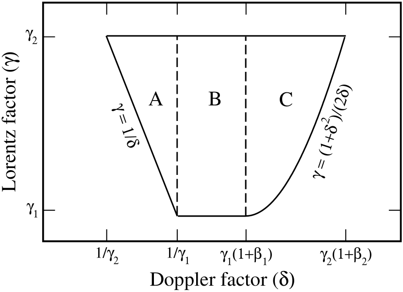
Figure 7: Plot of Lorentz factor versus Doppler factor illustrating integration limits for determining $P_{\delta}$ (see equation A5). For a particular value of $\delta$, the integration limits on $\gamma$ are defined by the polygonal region (i.e., the lower integration limit is equal to $\delta^{-1}$ in region A, $\gamma_{1}$ in region B, and $(1+\delta^{2})/2\delta$ in region C.)

A.3 Case 3: Power Law Lorentz Factor Distributions

A.3.1 Power law distribution of the form $P_{\gamma}(\gamma)\propto\gamma$

For the case $a=+1$ we have

$$P_{\gamma}(\gamma)=\cases{2\left(\gamma_{2}^{2}-\gamma_{1}^{2}\right)^{-1}&for $\gamma_{1}\leq\gamma\leq\gamma_{2}$\cr 0&elsewhere.}$$ (A11)

Substituting this into equation (A5) gives

$$P_{\delta}(\delta;a=+1)={2\over\delta^{2}\left(\gamma_{2}^{2}-\gamma_{1}^{2}\right)}\times\cases{\gamma_{2}\beta_{2}-{\sqrt{1-\delta^{2}}\over\delta}&for $\quad\gamma_{2}^{-1}\leq\delta<\gamma_{1}^{-1}$\cr\gamma_{2}\beta_{2}-\gamma_{1}\beta_{1}&for $\quad\gamma_{1}^{-1}\leq\delta<\gamma_{1}(1+\beta_{1})$\cr\gamma_{2}\beta_{2}-{\delta^{2}-1\over 2\delta}&for $\quad\gamma_{1}(1+\beta_{1})\leq\delta\leq\delta_{max}$\cr 0&elsewhere.}$$ (A12)

A.3.2 Power law distribution of the form $P_{\gamma}(\gamma)\propto\gamma^{-1}$

For the case $a=-1$ we have

$$P_{\gamma}(\gamma)=\cases{\left(\gamma\ln{\left|{\gamma_{2}/\gamma_{1}}\right|}\right)^{-1}&for $\gamma_{1}\leq\gamma\leq\gamma_{2}$\cr 0&elsewhere.}$$ (A13)

We obtain

$$P_{\delta}(\delta;a=-1)={1\over\delta^{2}\ln{\left|{\gamma_{2}/\gamma_{1}}\right|}}\times\cases{\arctan{\left[\delta\over\sqrt{1-\delta^{2}}\right]}-\arctan{\left[1\over\gamma_{2}\beta_{2}\right]}&for $\quad\gamma_{2}^{-1}\leq\delta<\gamma_{1}^{-1}$\cr\arctan{\left[1\over\gamma_{1}\beta_{1}\right]}-\arctan{\left[1\over\gamma_{2}\beta_{2}\right]}&for $\quad\gamma_{1}^{-1}\leq\delta<\gamma_{1}(1+\beta_{1})$\cr\arctan{\left[2\delta\over\delta^{2}-1\right]}-\arctan{\left[1\over\gamma_{2}\beta_{2}\right]}&for $\quad\gamma_{1}(1+\beta_{1})\leq\delta\leq\delta_{max}$\cr 0&elsewhere.}$$ (A14)

For large $\gamma_{2}$ and $\gamma_{1}\simeq 1$, this reduces to:

$$P_{\delta}(\delta;a=-1)={1\over\delta^{2}\ln{\left|{\gamma_{2}}\right|}}\times\cases{\arctan{\left[\delta\over\sqrt{1-\delta^{2}}\right]}&for $\quad\gamma_{2}^{-1}\leq\delta<1$\cr\arctan{\left[2\delta\over\delta^{2}-1\right]}&for $\quad 1\leq\delta\leq 2\gamma_{2}$.}$$ (A15)

A.3.3 Power law distribution of the form $P_{\gamma}(\gamma)\propto\gamma^{-2}$

For the case $a=-2$, we have

$$P_{\gamma}(\gamma)=\cases{\gamma^{-2}\left(\gamma_{1}^{-1}-\gamma_{2}^{-1}\right)^{-1}&for $\gamma_{1}\leq\gamma\leq\gamma_{2}$\cr 0&elsewhere.}$$ (A16)

We obtain

$$P_{\delta}(\delta;a=-2)={1\over\delta^{2}\left(\gamma_{1}^{-1}-\gamma_{2}^{-1}\right)}\times\cases{\beta_{2}-\sqrt{1-\delta^{2}}&for $\quad\gamma_{2}^{-1}\leq\delta<\gamma_{1}^{-1}$\cr\beta_{2}-\beta_{1}&for $\quad\gamma_{1}^{-1}\leq\delta<\gamma_{1}(1+\beta_{1})$\cr\beta_{2}-{\delta^{2}-1\over\delta^{2}+1}&for $\quad\gamma_{1}(1+\beta_{1})\leq\delta\leq\delta_{max}$\cr 0&elsewhere.}$$ (A17)

For large $\gamma_{2}$ and $\gamma_{1}\simeq 1$, this reduces to:

$$P_{\delta}(\delta;a=-2)\simeq{1\over\delta^{2}}\times\cases{1-\sqrt{1-\delta^{2}}&for $\quad\gamma_{2}^{-1}\leq\delta<1$\cr 2\left(\delta^{2}+1\right)^{-1}&for $\quad 1\leq\delta<2\gamma_{2}$.}$$ (A18)

Appendix B BEAMED LUMINOSITY FUNCTIONS OF JET POPULATIONS WITH A POWER-LAW DISTRIBUTION OF LORENTZ FACTORS

For $\gamma_{1}\neq 1$ , the form of the beamed luminosity function is:

$$\scriptsize\Phi(L)={k_{1}L^{-B}}\times\cases{0\;,&$\quad L<L_{min}$\cr F[(L/{\cal L}_{1})^{1/p}]-F[\gamma_{2}^{-1}],&$\quad L_{min}\leq L<L_{5}$\cr G[(L/{\cal L}_{1})^{1/p}]+F[\gamma_{1}^{-1}]-F[\gamma_{2}^{-1}]-G[\gamma_{1}^{-1}],&$\quad L_{5}\leq L<L_{6}$\cr H[(L/{\cal L}_{1})^{1/p}]+F[\gamma_{1}^{-1}]-F[\gamma_{2}^{-1}]+G[\gamma_{1}+\gamma_{1}\beta_{1}]-G[\gamma_{1}^{-1}]-H[\gamma_{1}+\gamma_{1}\beta_{1}],&$\quad L_{6}\leq L<L_{4}$\cr F[\gamma_{1}^{-1}]-F[\gamma_{2}^{-1}]+G[\gamma_{1}+\gamma_{1}\beta_{1}]-G[\gamma_{1}^{-1}]+H[\delta_{max}]-H[\gamma_{1}+\gamma_{1}\beta_{1}],&$\quad L_{4}\leq L<L_{3}$\cr-F[(L/{\cal L}_{2})^{1/p}]+F[\gamma_{1}^{-1}]+G[\gamma_{1}+\gamma_{1}\beta_{1}]-G[\gamma_{1}^{-1}]+H[\delta_{max}]-H[\gamma_{1}+\gamma_{1}\beta_{1}],&$\quad L_{3}\leq L<L_{7}$\cr-G[(L/{\cal L}_{2})^{1/p}]+G[\gamma_{1}+\gamma_{1}\beta_{1}]+H[\delta_{max}]-H[\gamma_{1}+\gamma_{1}\beta_{1}],&$\quad L_{7}\leq L<L_{8}$\cr-H[(L/{\cal L}_{2})^{1/p}]+H[\delta_{max}],&$\quad L_{8}\leq L\leq L_{max}$\cr 0\;,&$\quad L>L_{max}$.}$$ (B1)

If $\gamma_{1}=1$, then $L_{5}=L_{6}={\cal L}_{1}$, and $L_{7}=L_{8}={\cal L}_{2}$, and equation (B1) reduces to:

$$\Phi(L)=k_{1}L^{-B}\times\cases{0\;,&$\quad L<L_{min}$\cr F[(L/{\cal L}_{1})^{1/p}]-F[\gamma_{2}^{-1}],&$\quad L_{min}\leq L<{\cal L}_{1}$\cr H[(L/{\cal L}_{1})^{1/p}]-H[1]+F[1]-F[\gamma_{2}^{-1}]&$\quad{\cal L}_{1}\leq L<L_{4}$\cr F[1]-F[\gamma_{2}^{-1}]+H[\delta_{max}]-H[1],&$\quad L_{4}\leq L<L_{3}$\cr-F[(L/{\cal L}_{2})^{1/p}]+F[1]+H[\delta_{max}]-H[1],&$\quad L_{3}\leq L<{\cal L}_{2}$\cr-H[(L/{\cal L}_{2})^{1/p}]+H[\delta_{max}],&$\quad{\cal L}_{2}\leq L\leq L_{max}$\cr 0\;,&$\quad L>L_{max}$\cr}$$ (B2)

The functions $F(x)$, $G(x)$, and $H(x)$ are tabulated in the following sections for various integer values of $a$ and $Cp$. They are grouped by particular values of $a$, where $P_{\gamma}(\gamma)\propto\gamma^{a}$ in the jet population, and are further subdivided by particular values of the product $Cp$ (see eq. 8).

B.1 Power-Law Lorentz Factor Distribution of the form $P_{\gamma}(\gamma)\propto\gamma$

When $a=+1$ we have:

$$F(x)={2\over\gamma_{2}^{2}-\gamma_{1}^{2}}\times\cases{\gamma_{2}\beta_{2}\ln{|x|}+\arcsin{x}+{\sqrt{1-x^{2}}\over x},&if $\quad Cp=0$\cr\gamma_{2}\beta_{2}x-\sqrt{1-x^{2}}-\ln{\left|{x\over 1+\sqrt{1-x^{2}}}\right|},&if $\quad Cp=1$\cr{1\over 2}\gamma_{2}\beta_{2}x^{2}-{1\over 2}\arcsin{x}-{x\over 2}\sqrt{1-x^{2}},&if $\quad Cp=2$\cr{1\over 3}\gamma_{2}\beta_{2}x^{3}+{1\over 3}(1-x^{2})^{3/2},&if $\quad Cp=3$,}$$ (B3)

$$G(x)={2\left(\gamma_{2}\beta_{2}-\gamma_{1}\beta_{1}\right)\over\left(\gamma_{2}^{2}-\gamma_{1}^{2}\right)}\times\cases{\ln{|x|},&if $\quad Cp=0$\cr{x^{Cp}\over Cp},&if $\quad Cp=1,2,3$,}$$ (B4)

$$H(x)={2\over\gamma_{2}^{2}-\gamma_{1}^{2}}\times\cases{\gamma_{2}\beta_{2}\ln{|x|}-{x\over 2}-{1\over 2x},&if $\quad Cp=0$\cr\gamma_{2}\beta_{2}x-{x^{2}\over 4}-{1\over 2}\ln{|x|},&if $\quad Cp=1$\cr{\gamma_{2}\beta_{2}x^{Cp}\over Cp}-{x^{Cp+1}\over 2(Cp+1)}-{x^{Cp-1}\over 2(Cp-1)},&if $\quad Cp=2,3$.}$$ (B5)

B.2 Uniform Lorentz factor distribution of the form $P_{\gamma}(\gamma)=constant$

In the case of a uniform $\gamma$ distribution ($a=0$), we have

$$F(x)={1\over\gamma_{2}-\gamma_{1}}\times\cases{x\ln{\left|{x\;\delta_{max}\over 1+\sqrt{1-x^{2}}}\right|}-\arcsin{x},&if $\quad Cp=1$\cr{1\over 2}\sqrt{1-x^{2}}+{x^{2}\over 2}\ln{\left|{x\delta_{max}\over 1+\sqrt{1-x^{2}}}\right|},&if $\quad Cp=2$\cr{x\over 6}\sqrt{1-x^{2}}-{1\over 6}\arcsin{x}+{x^{3}\over 3}\ln{\left|{x\delta_{max}\over 1+\sqrt{1-x^{2}}}\right|}&if $\quad Cp=3$,}$$ (B6)

$$G(x)={x^{Cp}\ln{\left|\delta_{max}\over\gamma_{1}(1+\beta_{1})\right|}\over(\gamma_{2}-\gamma_{1})Cp},\quad{\rm if}\quad Cp=1,2,3,$$ (B7)

$$H(x)={x^{Cp}\left(1+Cp\;\ln{\left|\delta_{max}/x\right|}\right)\over(\gamma_{2}-\gamma_{1})(Cp)^{2}}\quad\quad{\rm if}\quad Cp=1,2,3.$$ (B8)

There are no analytical expressions possible when $a=0$ and $Cp=0$.

B.3 Power-Law Lorentz Factor Distribution of the form $P_{\gamma}(\gamma)\propto\gamma^{-1}$

When $a=-1$, we have

$$F(x)={1\over\ln{\left|\gamma_{2}/\gamma_{1}\right|}}\times\cases{x\left[\arctan{\left(x\over\sqrt{1-x^{2}}\right)}-\arctan{\left({1\over\gamma_{2}\beta_{2}}\right)}\right]+\sqrt{1-x^{2}},&if $\quad Cp=1$\cr{x^{2}\over 2}\left[\arctan{\left(x\over\sqrt{1-x^{2}}\right)}-\arctan{\left({1\over\gamma_{2}\beta_{2}}\right)}\right]+{x\over 4}\sqrt{1-x^{2}}-{1\over 4}\arcsin{[x]},&if $\quad Cp=2$\cr{x^{3}\over 3}\left[\arctan{\left(x\over\sqrt{1-x^{2}}\right)}-\arctan{\left({1\over\gamma_{2}\beta_{2}}\right)}\right]+{1\over 9}(x^{2}+2)\sqrt{1-x^{2}},&if $\quad Cp=3$,}$$ (B9)

$$G(x)={x^{Cp}\over Cp\ln{\left|\gamma_{2}/\gamma_{1}\right|}}\left[\arctan{\left({1\over\gamma_{1}\beta_{1}}\right)}-\arctan{\left({1\over\gamma_{2}\beta_{2}}\right)}\right],\quad{\rm if}\quad Cp=1,2,3,$$ (B10)

$$H(x)={1\over\ln{\left|\gamma_{2}/\gamma_{1}\right|}}\times\cases{x\left[\arctan{\left(2x\over x^{2}-1\right)}-\arctan{\left({1\over\gamma_{2}\beta_{2}}\right)}\right]+\ln{\left|x^{2}+1\right|},&if $\quad Cp=1$\cr{x^{2}\over 2}\left[\arctan{\left(2x\over x^{2}-1\right)}-\arctan{\left({1\over\gamma_{2}\beta_{2}}\right)}\right]+x-\arctan{x},&if $\quad Cp=2$\cr{x^{3}\over 3}\left[\arctan{\left(2x\over x^{2}-1\right)}-\arctan{\left({1\over\gamma_{2}\beta_{2}}\right)}\right]+{x^{2}\over 3}-{1\over 3}\ln{\left|x^{2}+1\right|},&if $\quad Cp=3$.}$$ (B11)

There are no analytical expressions possible when $a=-1$ and $Cp=0$.

B.4 Power-Law Lorentz Factor Distribution of the form $P_{\gamma}(\gamma)\propto\gamma^{-2}$

For the case $a=-2$, we have

$$F(x)={1\over\gamma_{1}^{-1}-\gamma_{2}^{-1}}\times\cases{(\beta_{2}-1)\ln{x}-\sqrt{1-x^{2}}+\ln{\left|1+\sqrt{1-x^{2}}\right|},&if $\quad Cp=0$\cr\beta_{2}x-{x\over 2}\sqrt{1-x^{2}}-{1\over 2}\arcsin{x},&if $\quad Cp=1$\cr{\beta_{2}x^{2}\over 2}+{1\over 3}(1-x^{2})^{3/2},&if $\quad Cp=2$\cr{\beta_{2}x^{3}\over 3}-{1\over 8}\arcsin{x}-{x\over 8}(2x^{2}-1)\sqrt{1-x^{2}},&if $\quad Cp=3$,}$$ (B12)

$$G(x)={(\beta_{2}-\beta_{1})\over\left(\gamma_{1}^{-1}-\gamma_{2}^{-1}\right)}\times\cases{\ln{|x|},&if $\quad Cp=0$\cr{x^{Cp}\over Cp},&if $\quad Cp=1,2,3$,}$$ (B13)

$$H(x)={1\over\gamma_{1}^{-1}-\gamma_{2}^{-1}}\times\cases{(\beta_{2}+1)\ln{x}-\ln{\left|1+x^{2}\right|},&if $\quad Cp=0$\cr(\beta_{2}-1)x+2\arctan{x},&if $\quad Cp=1$\cr{1\over 2}(\beta_{2}-1)x^{2}+\ln{\left|1+x^{2}\right|},&if $\quad Cp=2$\cr{1\over 3}(\beta_{2}-1)x^{3}+2x-2\arctan{x},&if $\quad Cp=3$.}$$ (B14)

References

- Jackson & Wall (1999) Jackson, C. A. & Wall, J. V. 1999, MNRAS, 304, 160
- Kellermann et al. (1998) Kellermann, K. I., Vermeulen, R. C., Zensus, J. A., & Cohen, M. H. 1998, AJ, 115, 1295
- Kellermann et al. (2003) Kellermann, K. I. et al, 2003, in preparation
- Kumar & Piran (2000) Kumar, P. & Piran, T. 2000, ApJ, 535, 152
- Lind & Blandford (1985) Lind, K. R. & Blandford, R. D. 1985, ApJ, 295, 358
- Lister & Marscher (1997) Lister, M. L. & Marscher, A. P. 1997, ApJ, 476, 572
- Taylor et al. (1996) Taylor, G. B., Vermeulen, R. C., Readhead, A. C. S., Pearson, T. J., Henstock, D. R., & Wilkinson, P. N. 1996, ApJS, 107, 37
- Urry & Padovani (1995) Urry, C. M. & Padovani, P. 1995, PASP, 107, 803
- Urry & Padovani (1991) Urry, C. M. & Padovani, P. 1991, ApJ, 371, 60
- Urry, Padovani, & Stickel (1991) Urry, C. M., Padovani, P., & Stickel, M. 1991, ApJ, 382, 501
- Urry & Shafer (1984) Urry, C. M. & Shafer, R. A. 1984, ApJ, 280, 569 (US84)
- Vermeulen & Cohen (1994) Vermeulen, R. C. & Cohen, M. H. 1994, ApJ, 430, 467
- Vermeulen et al. (2003) Vermeulen, R. C., & Britzen, S. 2003, in Radio Astronomy at the Fringe, Proceedings of a Workshop on Extragalactic Radio Sources held in Green Bank, WV, Oct 10-12, 2002, eds. J.A. Zensus, E. Ros, & M.H.C. Cohen, in press.
- Willott et al. (1998) Willott, C. J., Rawlings, S., Blundell, K. M., & Lacy, M. 1998, MNRAS, 300, 625
- Zensus et al. (2003) Zensus, J. A., et al. 2003, in Radio Astronomy at the Fringe, Proceedings of a Workshop on Extragalactic Radio Sources held in Green Bank, WV, Oct 10-12, 2002, eds. J.A. Zensus, E. Ros, & M.H.C. Cohen, in press.