The X-ray variability of the Narrow-Line Seyfert 1 galaxy IRAS 13224–3809 from an XMM-Newton observation

Abstract

We report on the XMM-Newton timing properties of the most X-ray variable, radio-quiet, Narrow-Line Seyfert 1 galaxy IRAS 13224–3809. IRAS 13224–3809 continues to display the extremely variable behavior that was previously observed with ROSAT and ASCA; however, no giant, rapid flaring events are observed. We detect variations by a factor as high as $\sim$8 during the 64 ks observation, and the variability is persistent throughout the light curve. Dividing the light curve into 9 minute segments we found almost all of the segments to be variable at $>$ 3 $\sigma$. When the time-averaged cross-correlation function is calculated for the 0.3–0.8 keV band with the 3–10 keV band, the cross-correlation profile is skewed indicating a possible smearing of the signal to longer times (soft band leading the hard). A correlation between count rate and hardness ratio is detected in four energy bands. In three cases the correlation is consistent with spectral hardening at lower count rates which can be explained in terms of a partial-covering model. The other band displays the reverse effect, showing spectral hardening at higher count rates. We can explain this trend as a more variable power-law component compared to the soft component. We also detect a delay between the 0.3–1.5 keV count rate and the 0.8–1.5 keV to 0.3–0.8 keV hardness ratio, implying flux induced spectral variability. Such delays and asymmetries in the cross correlation functions could be suggesting reprocessing of soft and hard photons. In general, much of the timing behavior can be attributed to erratic eclipsing behavior associated with the partial covering phenomenon, in addition to intrinsic variability in the source. The variability behavior of IRAS 13224–3809 suggests a complicated combination of effects which we have started to disentangle with this present analysis.

1 Introduction

The Narrow-Line Seyfert 1 galaxy (NLS1) IRAS 13224–3809 is one of the most exciting NLS1s to study as it exhibits many of the extreme characteristics that make this class of objects so interesting. Strong Fe II emission in its optical spectrum (Boller et al. 1993); a giant soft X-ray excess (Boller et al. 1996; Otani et al. 1996; Leighly 1999a; Boller et al. 2003); and extreme, rapid, and persistent variability in X-rays (Boller et al. 1996; Boller et al. 1997; Otani et al. 1996; Leighly 1999b), are all traits of IRAS 13224–3809.

Boller et al. (2003; hereafter Paper I) presented an array of new spectral complexities observed in an XMM-Newton observation. In addition to the strong soft excess component they detected a broad absorption feature at $\sim$1.2 keV, first seen with ASCA (Otani et al. 1996; Leighly et al. 1997), and most probably due to Fe L absorption (Nicastro et al. 1999). Moreover, a sharp spectral power-law cut-off at $\sim$8.1 keV was discovered, similar to the power-law cut-off at 7.1 keV observed in the NLS1 1H 0707-495 (Boller et al. 2002).

In this paper we have examined the timing properties of IRAS 13224–3809 as observed with XMM-Newton and have related them to the spectral properties discussed in Paper I. In the next section we will discuss the data analysis before presenting the timing properties: OM light curve (Section 3), X-ray light curve and flux variability (Section 4), spectral variability (Section 5), and a discussion of our results in Section 6. A value for the Hubble constant of $H_{0}$=$\rm 70\ km\ s^{-1}\ Mpc^{-1}$ and for the cosmological deceleration parameter of $q_{0}=\rm\frac{1}{2}$ have been adopted throughout. Fluxes and luminosities were derived assuming the partial-covering fit described in Paper I and further assuming isotropic emission.

2 The X-ray observation and data analysis

IRAS 13224–3809 was observed with XMM-Newton (Jansen et al. 2001) for $\sim$64 ks during revolution 0387 on 2002 January 19. All instruments were functioning normally during this time. A detailed description of the observation and data analysis was presented in Paper I, and we will briefly summarize details which are important to the analysis here.

The EPIC pn camera (Strüder et al. 2001) was operated in full-frame mode, and the two MOS cameras (MOS1 and MOS2; Turner et al. 2001) were operated in large-window mode. All of the EPIC cameras used the medium filter. The Observation Data Files (ODFs) were processed to produce calibrated event lists in the usual manner using the XMM-Newton Science Analysis System (SAS) v5.3. Light curves were extracted from these event lists to search for periods of high background flaring. A significant background flare was detected in the EPIC cameras approximately 20 ks into the observation and lasting for $\sim$5 ks. Although the total counts at flare maximum were at least a factor of 3 lower than the source counts, the segment was excluded during most of the analysis. However, when calculating cross correlation functions, we kept all of the data to avoid dealing with gapped time series. The total amount of good exposure time selected from the pn camera was 55898 s.

3 The UV Observation

The Optical Monitor (OM; Mason et al. 2001) collected data in the fast mode through the UVW2 filter (1800–2250Å) for about the first 25 ks of the observation. For the remainder of the observation the OM was operated in the grism mode. In total, seven photometric images were taken, each exposure lasting 2000 s.

The apparent UVW2 magnitude is 15.21 $\pm$ 0.07 corresponding to a band flux of 4.56 $\times$ 10^-15 erg s^-1 cm^-2 Å^-1. The flux is consistent with previous UV observations with IUE (Mas-Hesse et al. 1994; Rodr’ıguez et al. 1997). The RMS scatter in the seven hour OM light curve is less than 0.5%. This agrees with the limits on rapid variability from the optical band (Young et al. 1999; but see Miller et al 2000).

The optical to X-ray spectral index, $\alpha_{ox}$, was calculated using the definition

$$\alpha_{ox}=\frac{log(f_{2keV}/f_{1990\AA})}{log(\nu_{2keV}/\nu_{1990\AA})},$$

where $f_{2keV}$ and $f_{1990\AA}$ are the intrinsic flux densities at 2 keV and 1990 Å, respectively. The selection of the UV wavelength corresponds to the peak response in the UVW2 filter (212 nm). Under the assumption that the UV light curve remains constant during the second half of the observation, we determined an average power-law slope $<\alpha_{ox}>$ = –1.57. As the 2 keV X-ray flux varies, $\alpha_{ox}$ fluctuates from –1.47 in the high state, to –1.73 in the low state.

4 The X-ray Light Curves

In the remainder of the paper we will concentrate on the EPIC pn light curve due to its high signal-to-noise. We will make reference to the various flux states as they were defined in Paper I: high ($>$2.5 counts s^-1), low ($<$1.5 counts s^-1), and medium (1.5–2.5 counts s^-1). The MOS light curve was also analyzed and found to be entirely consistent with the pn results. In the interest of brevity, the MOS results will not be presented here.

4.1 Flux Variability

EPIC pn light curves of IRAS 13224–3809 in three energy bands are presented in Figure 1.

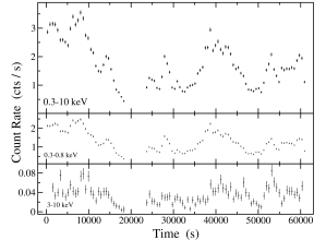
Figure 1: Three light curves of IRAS 13224–3809 in 600 s bins. The energy bands (and average count rates) are (from top-down): 0.3–10 (1.74), 0.3–0.8 (1.30), and 3–10 (0.03) keV. Zero seconds on the time axis marks the start of the observation at 03:15:02 on 2002–01–19. The region of high background flaring has been omitted.

The average count rate in the 0.3–10 keV energy band is (1.74 $\pm$ 0.05) counts s^-1. Variations by a factor of $\sim$8 occur during the observation. Using a 600 s bin size, the minimum and maximum 0.3–10 keV count rates are (0.44 $\pm$ 0.03) and (3.55 $\pm$ 0.08) counts s^-1, respectively. True to its strong soft-excess nature, IRAS 13224–3809 generates nearly three-quarters of the average count rate in the 0.3–0.8 keV band. Light curves were compared to a constant fit with a $\chi^{2}$ test. A constant fit could be rejected for all of the light curves at $>$3 $\sigma$ significance.

Giant-amplitude flaring events, as observed in the ROSAT and ASCA observations, are not present during this observation. In fact, the light curve appears to be in a period of relative quiescence compared to those earlier observations. The unabsorbed 0.3–2.4 keV flux is between (0.3–0.7) $\times$ 10^-11 erg s^-1 cm^-2 during the average low and high flux states. Extrapolation of the data from 0.3 keV to 0.1 keV allows us to estimate a 0.1–2.4 keV flux of (0.4–1.1) $\times$ 10^-11 erg s^-1 cm^-2. It is interesting to note that while the XMM-Newton light curve does not display giant flaring episodes, the flux during this observation is close to the $ROSAT$ HRI (0.1–2.4 keV) flux during the largest flaring events (3.3 $\times$ 10^-11 erg s^-1 cm^-2; Boller et al. 1997). Therefore, in comparison to the $ROSAT$ observations, IRAS 13224–3809 is in a relatively high flux state. In fact, the median HRI flux over the $ROSAT$ 30 day monitoring campaign was $\sim$ 0.2 $\times$ 10^-11 erg s^-1 cm^-2, while the average estimated 0.1–2.4 keV flux during this XMM-Newton observation is about a factor of three greater. It is not clear, with only the current observation in hand, whether this flux increase is a long-term change (i.e. lasting for periods of days-months), or if we are observing the AGN during some sort of extended outburst.

4.1.1 Rapid Variability

We conducted a search for the shortest time scales for which we could detect variability in IRAS 13224–3809 by employing the excess pair fraction method (Yaqoob et al. 1997). We constructed 90 light curves with time bin sizes from 6–1550 s and calculated the excess pair fraction (EPF) for each of them. The results are plotted in Figure 2. The dotted line in Figure 2 is the level of the EPF expected from Poisson noise. The measurements run into the Poisson noise for bin sizes less than $\sim$70 s. With a bin size of 90 s the source is variable at greater than 3 $\sigma$.

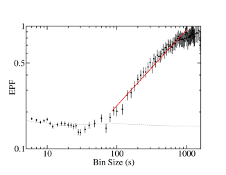
Figure 2: The EPF as a function of bin width calculated for IRAS 13224–3809. The dotted line is the estimated level of the EPF expected from Poisson noise. The faint, solid line is a power-law fit to the 85–1000s (1.2 $\times$ 10^-2–10^-3 Hz) region, with a normalisation of 0.013${}^{+0.003}_{-0.002}$ and an index of 0.619 $\pm$ 0.036. This measured index is related to the power-law index of the power spectrum ($\alpha$), and consistent with $\alpha$ = -1.619 (see Yaqoob et al. 1997 for a detailed explanation).

We searched further for indications of rapid variability by determining the shortest doubling times; that is, by searching for the shortest time interval in which the count rate doubles. Count rate doubling times on the order of 800 s were reported during the $ROSAT$ observations and as low as 400 s during the $ASCA$ observation. With this most recent XMM-Newton observation, numerous such events are found on time scales between 300–800 s, and the shortest measured doubling time is about 270 s.

4.1.2 Persistent Variability

Clearly absent from the light curves are the giant and rapid flux outbursts that one has come to expect from IRAS 13224–3809 (Boller et al. 1993; Otani et al. 1996; Boller et al. 1997; Leighly 1999b; Dewangan et al. 2002). In the galaxy’s defence, long monitoring with ROSAT (Boller et al 1997) suggests that such flaring events occur every few days; hence, were probably missed by this short ($<$ 1 day) observation. However, short time binning of the light curve ($<$100 s) reveals persistent variability.

With 60 s binning of the data, we searched for segments of quiescence in the light curve. Dividing the light curve into 10 minute segments, we used the $\chi^{2}$ test to search for global variability in each segment and found all of the segments to be variable at $>$3 $\sigma$ significance. In this manner, we worked our way through shorter time segments. Examining 9 minute segments we found that 101 of 103 segments were variable at $>$3 $\sigma$ significance (the other 2 segments were variable at $>$2.6 $\sigma$). The shortest segment size tested was 5 minutes, for which we determined that $\sim$62% (115/187) of the segments showed variability at a significance level $>$2.6 $\sigma$. The variable segments do not appear to be associated with a particular flux state. About 65% of the high flux segments and 57% of the low flux segments displayed variability.

The persistent variability on such short time scales disfavors the idea that the variability is dominated by intrinsic disc instabilities, primarily because of the much longer time scales expected for this process (Boller et al. 1997). This is, perhaps, inline with the lack of simultaneous UV fluctuations (as found in the OM light curve). Some AGN models predict that the UV and soft X-ray emission are the same physical process, namely thermal emission from the accretion disc (Big Blue Bump). Bearing this in mind, one would expect that the UV and soft X-rays should vary on similar time scales if the variability were due primarily to disc instabilities. Since this is not the case for IRAS 13224–3809 (in addition to the high thermal temperature derived in Paper I), there must be some other overriding process responsible for the rapid X-ray variability on time scales of minutes.

The persistent variability on such short time scales is also in contradiction with the idea that the variability arises from a single, rotating hot spot on the disc. Furthermore, there are no detectable temperature changes in the soft spectrum, as would be expected due to beaming effects. However, the hot spot model cannot be dismissed as the cause of the large-amplitude fluctuations during flaring episodes. The persistent variability on time scales of minutes is most likely due to a combination of effects, and no one origin (e.g. disc instabilities, coronal flaring, hot spots) can be definitively ruled out.

4.1.3 Radiative Efficiency

If we assume photon diffusion through a spherical mass of accreting matter we can estimate the radiative efficiency, $\eta$, from the expression $\eta$ $>$ 4.8 $\times$ 10${}^{-43}(\Delta L/\Delta t)$ (Fabian 1979; see also Brandt et al. 1999 for a discussion of important caveats), where $\Delta L$ is the change in luminosity, and $\Delta t$ is the time interval in the rest-frame of the source. From both ROSAT (Boller et al. 1997) and ASCA (Otani et al. 1996) observations of IRAS 13224–3809, a radiative efficiency exceeding the maximum Schwarzschild black hole radiative efficiency ($\eta$$=$0.057) was determined. It is tempting to attribute this result to accretion onto a Kerr black hole, or anisotropic emission, or X-ray hot spots on the disc.

We calculated the radiative efficiency at several points in the 200 s binned 0.3–10 keV light curve. From the mean unabsorbed luminosity (6 $\times$ 10⁴³ erg s^-1) and average count rate (1.74 $\pm$ 0.05 counts s^-1) we were able to calculate a conversion factor between count rate and luminosity (1 count s^-1 = 3.4 $\times$ 10⁴³ erg s^-1) and hence, we are able to calculate the luminosity rate of change from the observed change in count rate. Minimum and maximum count rates and times were averaged over at least two bins (ideally three). The regions selected correspond to the most rapid changes in count rate (either rising or falling), and they occupy various regions in the light curve (i.e. regions were selected in the high, low, and medium flux states, as well as events transcending the different flux states).

The most rapid rate of change was $(\Delta L/\Delta t)$ = (4.10 $\pm$ 0.91) $\times$ 10⁴⁰ erg s^-2 corresponding to a radiative efficiency of $\eta$ $>$ 0.020. Averaging over all ten selected regions we determine an average radiative efficiency of $\eta$ $>$ 0.013. No clear trend is seen between the value of $\eta$ and the flux state of the object from which the measurement was made. Since the calculated $\eta$ is a lower limit, our small value is not inconsistent with the $\eta$ calculated from the ROSAT or ASCA observations; nevertheless, it is nearly a factor of 10 smaller, and we are clearly consistent with the efficiency regime of a Schwarzschild black hole. It would stand to reason that we do not necessarily have a Kerr black hole in IRAS 13224–3809 since radiative efficiency limits in excess of the Schwarzschild limit are only found in the ROSAT (Boller et al. 1997) and ASCA (Otani et al. 1996) observations during periods of giant flaring outbursts. The large values of $\eta$ found in past observations are probably due to radiative boosting or anisotropic emission during the flaring events.

4.1.4 Correlations among the light curves

Several light curves in different energy bands were produced and compared with each other, and found to be correlated. The significance of the correlation was measured with the Spearman rank correlation coefficient (Press et al. 1992; Wall 1996). All of the light curves are well correlated with each other at $>$99.9% confidence.

Given the variability in all the light curves, and the significant correlation amongst all of them, it was natural to search for leads or lags by calculating the cross correlation function (CCF). We calculated CCFs between all the light curves and we present six of them in Figure 4.

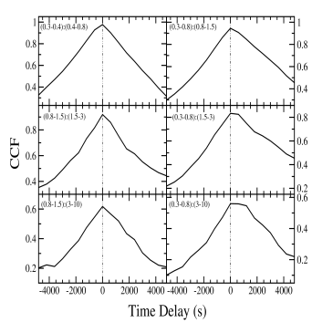
Figure 3: Six of the CCFs calculated from the light curves with 600s binning. The energy bands being cross correlated are shown in the top left of each window. The calculations were conducted such that a positive shift in time would indicate a lag of the second energy band.

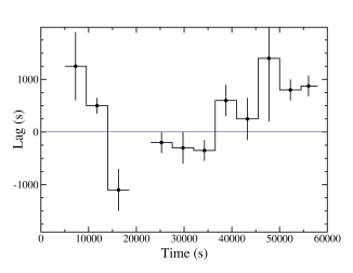
Figure 4: The lag measured between the 3–10 keV and 0.3–0.8 keV light curves, in 4500 s intervals, over the duration of the observation. The lag alternates in such a way that at times the soft band leads the hard (positive lag), and at other times, the hard leads the soft (negative lag). The time interval during which the background flare occurs has been omitted.

Most of the cross correlations are symmetric with a peak corresponding to zero time delay. However, when the soft 0.3–0.8 keV band is cross correlated with harder energy bands (right column of Figure 4), the CCFs become broad and somewhat flat-topped with a noticeable asymmetry toward longer lags. Because the time sampling is sufficiently fast to resolve the variations in the light curves, it is the width of the ACF that ultimately limits the resolution of the CCF. The soft light curve has a red power spectrum (a power-law fit to the power spectrum has an index of $\sim$ -2; see Figure 2), giving an ACF that is quite broad. The pronounced asymmetry of the CCF suggests we are barely resolving a lag between the two light curves. Using the centroid of the CCF yields a lag of the 3–10 keV band by 460 $\pm$ 175 s. The other two CCFs in the right column of Figure 4 also reveal a slight asymmetry. The CCFs peak at a lag of zero, but the asymmetry suggests the hard bands lag the soft. The pronounced asymmetry of the 3–10 keV versus the 0.3–0.8 keV CCF warranted more attention.

Careful inspection of the light curves indicate that the hard X-rays do not always lag the soft; in some cases it appears that the reverse is true. To investigate further, we cut the soft and hard light curves into 12 segments, each 4500 s in duration with 50% overlap between them (so only ever other segment is independent). We then computed the CCF in each of these shorter light curves. The results confirmed our visual suspicion — in some cases the hard X-rays lead the soft while at other times it lags. The results are shown in Figure 4. The lags span approximately -1100 s to +1400 s and appear to be mildly correlated with the soft X-rays in the sense that when the soft X-rays are strong, the hard lags the soft. The lag is positive more often than negative in our light curves, explaining why the full CCFs show a slight positive lag. Error bars on the lags were determined via a Monte Carlo technique: 5000 simulated soft and hard light curves were generated by varying every observed datum according to a Gaussian distribution whose standard deviation was equal to the uncertainty in the observation. The CCF was computed for each light curve pair and the peak recorded. The width of the distribution of the 5000 peaks was used to estimate the uncertainty in the lag. This was repeated for each of the 12 light curve segments. The perceived lags and leads are likely due to a physical separation between the soft and hard emitting regions and/or reprocessing.

5 Detection of significant and rapid Spectral Variability

From the available light curves we calculated seven hardness ratios by the definition $(H-S)/(H+S)$, where $H$ and $S$ are the count rates in the hard and soft bands, respectively. With this formalism, the value of the hardness ratio will be between $-1$ and +1, and the harder spectra will have more positive values. A typical hardness ratio is shown versus time in Figure 5. In this case $H$=1.5–10 keV and $S$= 0.3–1.5 keV. All seven ratios show similar time variability to the hardness ratio in Figure 5, albeit, some with poorer signal-to-noise. In addition, each hardness ratio curve was tested for global variability via a $\chi$² test. In all cases, the hardness ratios were inconsistent with a constant at greater than 2.6 $\sigma$.

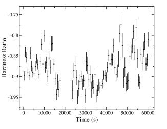
Figure 5: A typical hardness ratio variability curve. In this example $H$=1.5–10 keV and $S$=0.3–1.5 keV (see text for details). Zero seconds on the time axis marks the start of the observation at 03:15:02 on 2002–01–19. The region of high background flaring has been omitted.

The spectral variability depicted in Figure 5 is significant and rapid. In addition, the variability appears to intensify after about 40 ks into the observation. With the multiple spectral components required in the spectral model, isolating the location of the spectral variability is challenging.

We notice in Figure 1 that the overall trend in the count rate light curves is very similar between different energy bands; however, on closer inspection it becomes noticeable that the amplitude of the variations is different. To illustrate this observation better we produce normalised light curves in four energy bands, and in 10 ks bins (Figure 6). It becomes clear with this manner of binning that the amplitude of the flux variations are different among the energy bands, and indeed, there does appear to be a significant increase in the 3–10 keV flux after $\sim$40 ks.

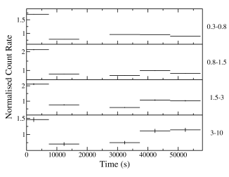
Figure 6: Four normalised X-ray light curves in various energy bands, and in 10 ks bins. After $\sim$40 ks, the amplitude of the fluctuations becomes greater in the 3–10 keV band then in the softer energy bands. Note that although the count rate error bars are plotted, they are too small to see in some of the light curves.

We searched for the source of the spectral variability further by calculating the fractional variability amplitude (F_var) following Edelson et al. (2002). The results are shown in Figure 7 using 200 s binning of the light curves.

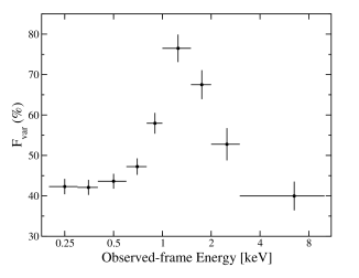
Figure 7: F_var calculated in nine energy bins between 0.2 and 10 keV. The light curves used were in bins of 200s.

Most of the variability is observed between 0.8 and 2 keV. This region is quite complex as it includes the broad Fe L absorption feature, and the point where the blackbody and power-law components intersect (see Paper I); hence, it is difficult to isolate any one component.

A difference spectrum (high-low) also confirms the spectral variability. A power-law is a good fit to the difference spectrum over the 1.3–8 keV band.

5.1 Flux correlated spectral variability

Given the reasonable agreement in the appearance of the hardness ratios and the light curves we searched for common trends in hardness ratio versus count rate plots. Using the Spearman rank correlation coefficient to test for correlations, four of the hardness ratios were found to be correlated with the light curves at more than 99.5% confidence. These four hardness ratios are plotted against the count rate in Figure 8. The four flux correlated hardness ratios are ($H$:$S$):
(1) (3–10):(0.3–0.8),
(2) (3–10):(1.5–3),
(3) (0.8–1.5):(0.3–0.8),
(4) (3–10):(0.8–1.5).
The count rates used are the summation of $H$ and $S$.

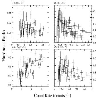
Figure 8: Four hardness ratios correlated with count rates. The bands used are show in the upper left of each panel. The count rates used are the summation of $H$ and $S$.

As can be seen from Figure 8, in four cases the spectral variability is correlated with the variability in the count rate. In three cases, spectral hardening was observed during periods of lower count rates. This general effect has been observed previously in IRAS 13224–3809 (Dewangan et al. 2002), as well as in other AGN, for example: MCG–6–30–15 (Lee et al. 2000), NGC 5548 (Chiang et al. 2000), 3C273 (Turner et al. 1990), and NGC 7314 (Turner 1987). The trend is a more common feature among X-ray novae (see Tanaka & Shibazaki 1996). Such a trend is predicted by the partial-covering model, and is further supported by the spectral analysis of IRAS 13224–3809 in Paper I (see their figure 7). However, the hardness ratio (0.8–1.5):(0.3–0.8) (lower left panel of Figure 8) shows the reverse effect – increased intensity when the spectrum is hard. Such a relation was also found in the radio-loud NLS1 PKS 0558–504 (Gliozzi et al. 2001). In that object, the hardening with increased flux was interpreted as an additional hard component due to a radio jet. This is probably not the case for IRAS 13224–3809 since it is radio-quiet and since the unusual hardness pattern is only observed over a small energy range. Since the 0.8–1.5 keV energy band is very complicated due to the comparable contributions from the thermal, power-law, and Fe L components, it is difficult to isolate or eliminate any one of these components. An alternative explanation for the observed trend is that each spectral component varies differently (or not at all) with changing flux. For example, the spectral variability in the Fe L could be independent of the flux. Similarly, the continuum in this band could also be independent of the flux changes and of the Fe L. However, when these possibly independent behaviors are combined, the trend presented in Figure 8 (lower left panel) arises. A more likely picture is that the intrinsic power-law is more variable than the soft component. This is supported somewhat by Figure 6, and we provide further evidence in support of this claim in Table 1. We modelled the 0.2–7 keV spectrum in various flux states (flux states are defined in Section 4 and in Paper I). In Table 1 we show the unabsorbed fluxes of the power-law and blackbody components in the 0.8–1.5 keV band. It is clear that the power-law does in fact show larger amplitude variations in this energy band. While the difference between the blackbody flux in the low and high state is $\sim$2.5, the power-law flux changes by more than a factor of 7. This is most likely the cause for the trend observed in the lower left panel of Figure 8.

Table 1: Comparison of the blackbody and power-law unabsorbed fluxes in the 0.8–1.5 keV band. Fluxes are in units of 10^-13 erg s^-1 cm^-2. The associated uncertainty in the fluxes is derived from the uncertainty in the count rates, and it is shown in brackets. The fourth column is the ratio of power-law flux over blackbody flux (column 3/column 2).

Flux State	Blackbody Flux	Power-law Flux	Ratio
High	7.97 (0.18)	5.00 (0.11)	0.63
Medium	4.89 (0.14)	2.41 (0.07)	0.49
Low	2.95 (0.20)	0.67 (0.05)	0.23

5.2 A possible lag between flux variations and spectral variations

Further complexities arise when we scrutinize the 0.3–1.5 keV light curve and spectral variations in greater detail. We calculated the cross correlation function of the 0.3–1.5 keV light curve versus the 0.8–1.5 keV to 0.3–0.8 keV hardness ratio variability curve. The cross correlation is presented in Figure 9, and indicates that the hardness ratio curve lags behind the light curve by 2000${}^{+1500}_{-2000}$ s. It is not clear whether this observation is supporting the reprocessing of soft photons idea, or indicating variability in the Fe L absorption feature, or some other effect.

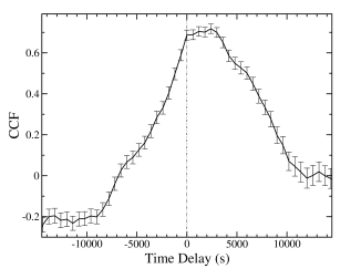
Figure 9: The cross correlation of the $H$=0.8–1.5 keV and $S$=0.3–0.8 keV light curve and hardness ratio variability curve. The CCF indicates a short delay between the two curves, such that, the hardness ratio curve lags behind the light curve.

Calculating light curve versus hardness ratio cross correlation functions for the other bands did not reveal any significant correlations. This could be an effect of the poorer signal-to-noise in those bands as opposed to some physical process. The band for which we have determined a lag is, perhaps not surprisingly, the highest signal-to-noise energy range.

6 Discussion

6.1 General Findings

We have presented the timing properties of the NLS1 IRAS 13224–3809 from a 64 ks XMM-Newton observation. Our findings are summarized below.

• As expected, persistent and rapid variability was prevalent, although no giant-amplitude variations are detected. The source was in a relatively high flux state compared to the ROSAT HRI observation.

• Unlike previous ROSAT and ASCA observations, the radiative efficiency was below the limit for a Schwarzschild black hole.

• Light curves in several bands were all well correlated. When any two light curves were cross correlated, most showed a symmetric correlation peaking at zero lag. However, when the time averaged 0.3–0.8 keV band was cross correlated with higher energy bands, an asymmetric cross-correlation profile was found. Further inspection indicates that the lag varies; in some cases the hard X-rays lead, and at other times they lag.

• Four of seven hardness ratio variability curves showed correlations with count rate fluctuations. Three of the four indicated spectral hardening at lower count rates, supporting the partial-covering scenario. The fourth hardness ratio, (0.8–1.5):(0.3–0.8), was characterized by hardening at higher count rates, most probably due to a more variable power-law component.

• The same hardness ratio, (0.8–1.5):(0.3–0.8), also shows a possible time delay compared to the light curve; thus, suggesting flux induced spectral variability.

6.2 Reprocessing Scenario

The basic idea in many AGN models is that high energy emission is produced in the accretion disc corona by Comptonisation of soft photons, which are likely thermal in nature. The detected positive lags (soft leads hard) in Figure 4 and 4, could be indicative of such a process. In this situation the time lag would be due to either a physical separation between the two emitting regions, or the reprocessing rate in the corona, or, most likely, a combination of the two. On the other hand, we also see evidence of the hard emission leading the soft (Figure 4 and 6), which could be occuring if high energy coronal photons are irradiating the disc and being Compton scattered. In this case, the perceived lag would most probably be due to a physical separation between the emitting regions, since the reprocessing rate is likely short due to the high densities in the disc. Interesting is the fact that the apparent leads and lags are alternating, indicating that both processes are occurring simultaneously but only one is dominating at a given time.

6.3 Future tests for the Partial-Covering and Discline Models

The partial-covering model (Holt et al. 1980; Boller et al. 2002; Tanaka et al 2003) is a very good fit to the spectrum in Paper I. The fit can adequately describe the sharp spectral feature at 8.1 keV, and the absence of the Fe line expected from the fluorescent yield, all with a reasonable Fe overabundance. The panels in Figure 8 which demonstrate spectral hardening during states of lower intensity are fully consistent with the partial-covering scenario. Observations of the intensity recovering above the edge, and the detection of other edges (e.g. Ni spectroscopy), would validate the partial-covering scenario in IRAS 13224–3809.

The discline model (Fabian et al. 2002) also provided a good fit across the whole energy band to the data in Paper I, and without requiring extra absorption (albeit, with a large equivalent width for the broad Fe line). Such a model is not inconsistent with the observed flux and spectral variability in IRAS 13224–3809, nor is it inconsistent with the interpretation that the asymmetric cross correlation functions are a result of reprocessing of soft energy photons. We could test for the presence of the Fe line by measuring the depth of the edge feature at $\sim$ 8.1 keV in various flux or temporal states. The overwhelming strength of the proposed line suggests that the variations we have detected probably arise within the line. Therefore, one would expect that as the line profile changes so would the depth of the edge. A constant edge depth would be inconsistent with the discline interpretation. With the current photon statistics it is not possible to conduct such a test precisely.

In general, much of the timing behavior can be described in the context of the partial covering phenomenon, with intrinsic source variability being a secondary effect. The variability behavior of IRAS 13224–3809 suggests a complicated combination of effects which we have started to disentangle in this present analysis. A much longer observation with XMM-Newton, including the detection of a giant outburst event, would allow us to answer several of the questions raised during this most recent X-ray observation.

References

- [1] Boller Th., Trümper J., Molendi S., Fink H., Schaeidt S., Caulet A., & Dennefeld M., 1993, A&A, 279, 53
- [2] Boller Th., Brandt W. N., & Fink H., 1996, A&A, 305, 53
- [3] Boller Th., Brandt W. N., Fabian A. C., & Fink H. 1997, MNRAS, 289, 393
- [4] Boller Th., Fabian A. C., Sunyaev R., Trümper, J., Vaughan S., Ballantyne D. R., Brandt W. N., Keil R., & Iwasawa K., 2002, MNRAS, 329, 1
- [5] Boller Th., Tanaka Y., Fabian A., Brandt W. N., Gallo L., Anabuki N., Haba Y., & Vaughan S., 2003, MNRAS, 343, 89
- [6] Brandt W. N., Boller Th., Fabian A. C., & Ruszkowski M., 1999, MNRAS, 303, L58
- [7] Chiang J., Reynolds C. S., Blaes O. M., Nowak M. A., Murray N., Madejski G., Marshall H. L., & Magdziarz P., 2000, ApJ, 528, 292
- [8] Dewangan G. C., Boller Th., Singh K. P., & Leighly K. M., 2002, A&A, 390, 65
- [9] Edelson R., Turner T. J., Pounds K., Vaughan S., Markowitz A., Marshall H., Dobbie P., & Warwick R., 2002, ApJ, 568, 610
- [10] Fabian A. C., 1979, Proc. R. Soc. London, Ser. A, 366, 449
- [11] Fabian A. C., Ballantyne D. R., Merloni A., Vaughan S., Iwasawa K., & Boller Th., 2002, MNRAS, 331, 35
- [12] Gliozzi M., Brinkmann W., O’Brien P. T., Reeves J. N., Pounds K. A., Trifoglio M., & Gianotti F., 2001, A&A, 365, 128
- [13] den Herder J. W., Brinkman A. C., Kahn S. M., Branduardi-Raymont G., Thomsen K., Aarts H., Audard M., Bixler J. V., den Boggende A. J., Cottam J., et al. 2001, A&A, 365, 7
- [14] Holt S. S., Mushotzky R. F., Boldt E. A., Serlemitsos P. J., Becker R. H., Szymkowiak A. E., & White, N. E., ApJ, 241, 13
- [15] Jansen F., Lumb D., Altieri B., Clavel J., Ehle M., Erd C., Gabriel C., Guainazzi M., Gondoin P., Much R. et al., 2001, A&A, 365, 1
- [16] Lee J. C., Fabian A. C., Reynolds C. S., & Brandt W. N., 2000, MNRAS, 318, 857
- [17] Leighly K. M., Mushotzky, R. F., Nandra, K., & Forster, K., 1997, ApJ, 489, 25
- [18] Leighly K., 1999a, ApJS, 125, 317
- [19] Leighly K., 1999b, ApJS, 125, 297
- [20] Mas-Hesse J. M., Rodr\a’ıguez-Pascual P. M., Sanz Fern\a’andez de C\a’ordoba L., & Boller Th., 1994, A&A, 283, L9
- [21] Mason K. O., Breeveld A., Much R., Carter M., Cordova F. A., Cropper M. S., Fordham J., Huckle H., Ho C., Kawakami H. et al. 2001, A&A, 365, 36
- [22] Miller H. R., Ferrara E. C., McFarland J. P., Wilson J. W., Daya A. B., & Fried R. E., 2000, NewAR, 44, 539
- [23] Nicastro F., Fiore F., & Matt G., 1999, ApJ, 517, 108
- [24] Otani C., Kii T., & Miya K., 1996, MPE Report 263, 491
- [25] Press W. H., Teukolsky S. A., Vetterling W. T., & Flannery B. P., 1992, Numerical Recipes, Cambridge Univ. Press
- [26] Rodr\a’ıguez-Pascual P. M., Mas-Hesse J. M., & Santos-Lle\a’o M., 1997, A&A, 327, 72
- [27] Strüder L., Briel U., Dennerl K., Hartmann R., Kendziorra E., Meidinger N., Pfeffermann E., Reppin C., Aschenbach B., Bornemann W. et al., 2001, A&A, 365 18
- [28] Tanaka Y., Ueda Y., & Boller Th., 2003, MNRAS, 338, 1
- [29] Tanaka Y. & Shibazaki N., 1996, ARA&A, 34, 607
- [30] Turner M. J. L. et al., 1990, MNRAS, 244, 310
- [31] Turner M. J. L., Abbey A., Arnaud M., Balasini M. Barbera M., Belsole, E., Bennie P. J., Bernard J. P., Bignami G. F., Boer M. et al., 2001, A&A, 365, 27
- [32] Turner T. J., 1987, MNRAS, 226, 9
- [33] Wall J. V., 1996, QJRAS, 37, 519
- [34] Yaqoob T., McKernan B., Ptak A., Nandra K., & Serlemitsos P. J., 1997, ApJ, 490, 25
- [35] Young A. J., Crawford C. S., Fabian A. C., Brandt W. N., & O’Brien P. T., 1999, MNRAS, 304, 46