A Far-Ultraviolet Survey of 47 Tucanae. II. The Long-Period Cataclysmic Variable AKO 9

Abstract

We present time-resolved, far-ultraviolet (FUV) spectroscopy and photometry of the 1.1 day eclipsing binary system AKO 9 in the globular cluster 47 Tucanae. The FUV spectrum of AKO 9 is blue and exhibits prominent C iv and He ii emission lines. The spectrum broadly resembles that of long-period, cataclysmic variables (CVs) in the galactic field.

Combining our time-resolved FUV data with archival optical photometry of 47 Tuc, we refine the orbital period of AKO 9 and define an accurate ephemeris for the system. We also place constraints on several other system parameters, using a variety of observational constraints. We find that all of the empirical evidence is consistent with AKO 9 being a long-period dwarf nova in which mass transfer is driven by the nuclear expansion of a sub-giant donor star. We therefore conclude that AKO 9 is the first spectroscopically confirmed CV in 47 Tuc.

We also briefly consider AKO 9’s likely formation and ultimate evolution. Regarding the former, we find that the system was almost certainly formed dynamically, either via tidal capture or in a 3-body encounter. Regarding the latter, we show that AKO 9 will probably end its CV phase by becoming a detached, double WD system or by exploding in a Type Ia supernova.

1 Introduction

The dense cores of globular clusters are expected to contain numerous close binary systems (CBs) produced via dynamical 2- and 3-body interactions, such as tidal capture (Fabian, Pringle & Rees 1975). The resulting CB populations are key to our understanding of globular cluster evolution: by giving up gravitational binding energy to passing single stars, CBs provide the heat input that is needed to reverse core collapse and drive their host clusters towards evaporation (Hut et al. 1992).

Cataclysmic variables (CVs) are particularly important tracers of a cluster’s CB population. These systems are interacting binaries in which a main sequence or slightly evolved secondary star loses mass via Roche-lobe overflow to a white dwarf (WD) primary. CVs are important because they should be both numerous and relatively easy to find. For example, di Stefano & Rappaport (1994) predict the presence of well over 100 active CVs formed by tidal capture in 47 Tuc, roughly 45 of which should have accretion luminosities in excess of $10^{33}$ erg s^-1. However, early optical searches found only a handful of CVs in all globular clusters combined (e.g. Shara et al. 1996; Bailyn et al. 1996; Cool et al. 1998).

Recently, the hunt for CVs in globular clusters has become much more successful. On the one hand, deep Chandra imaging of several clusters has uncovered numerous X-ray sources, whose properties and (in some cases) optical counterparts are consistent with those expected for CVs (Grindlay et al. 2001a; Grindlay et al. 2001b; Pooley et al. 2002a; Pooley et al. 2002b; Heinke et al. 2003). On the other hand, we have recently begun a far-ultraviolet (FUV) survey of globular cluster cores, which is very well-suited to the task of discovering CVs (Knigge et al. 2002; hereafter Paper I).

The first target of our survey was 47 Tuc, for which we obtained time-resolved FUV imaging and slitless spectroscopy (the latter is feasible because the move to the FUV reduces the crowding in the core dramatically). Results from the imaging portion of these observations were presented in Paper I and already demonstrated the potential of the FUV waveband for CV searches: all previously suspected CVs in our field of view were found to have variable FUV counterparts, and several new CV candidates were detected. Following on from this, the present paper contains first results from the spectroscopic portion of our FUV survey of 47 Tuc. More specifically, we present time-resolved FUV spectroscopy (supported by optical and FUV time-resolved photometry) of the brightest FUV source in 47 Tuc, AKO 9.

The nature of AKO 9 has been a long-standing puzzle. It is known to be an eclipsing binary with an orbital period of about 1.1 days (Edmonds et al. 1996) and with a significant UV-excess (Aurière, Koch-Miramond & Ortolani 1989; Paper I). Claims that it is associated with an X-ray source in the cluster have been made (Aurière, Koch-Miramond & Ortolani 1989; Geffert, Aurière & Koch-Miramond 1997) and refuted (Verbunt & Hasinger 1998), but this particular controversy has now been settled by Chandra observations. These revealed that AKO 9 is an X-ray source, with $L_{x}\simeq 7.5\times 10^{30}$ erg s^-1 (Grindlay et al. 2001a). Finally, and most puzzlingly, Minniti et al.(1997) observed an ”unusual brightening” of AKO 9, during which the system’s U-band flux increased by 2 mag in less than two hours. If this brightening is interpreted as a genuine increase in the system’s luminosity, it poses serious problems for essentially all models for this system (e.g. Minniti et al 1997).

Here, we show that AKO 9 is a variable, blue emission line source, whose FUV spectrum and other characteristics securely identify it as a long-period, dwarf-nova-type CV. We also derive a precise orbital ephemeris for the system, which reveals that the brightening described by Minniti et al. (1997) was simply an eclipse egress observed at a time when AKO 9 was already in outburst.

2 Observations

2.1 Far-Ultraviolet Photometry and Slitless Spectroscopy

Our FUV survey of 47 Tuc consists of thirty orbits of STIS/HST observations, comprised of six epochs of five orbits each (HST program GO-8279). The first epoch took place in 1999 September, and the gap between the first and second epochs was roughly 11 months; the second through sixth observations all occurred within a space of about 9 days. In each observing epoch, we carried out FUV imaging and slitless spectroscopy. Typical exposure times in the FUV were 600 s for both spectroscopy and imaging. Our program is therefore sensitive to variability on time-scales ranging from minutes to months.

All of our FUV observations used the FUV-MAMA detectors and were taken through the F25QTZ filter. This filter blocks geocoronal Ly$\alpha$, OI 1304 Å and OI] 1356 Å emission which would otherwise produce a high background across the detector in our slitless spectroscopy. We used the G140L first-order grating for the spectroscopic observations, yielding a dispersion of 0.584 Å pixel^-1 and a spectral resolution corresponding to roughly 1.2 Å (FWHM). The effective bandpass with this instrumental set-up is roughly 1450 Å – 1800 Å for both imaging and spectroscopy.

The 1024$\times$1024 pixel FUV-MAMA detector covers approximately 25″$\times$25″, at a spatial resolution of about 0.043″ (FWHM). Our field of view (FoV) was chosen to overlap with archival HST observations of 47 Tuc and includes the cluster center. The calibration of the FUV imaging observations has already been described in Paper I, so we focus here on the extraction and calibration of the FUV spectra of AKO 9.

Figure 1 shows an example of the slitless spectra we obtained. Each trail in this figure corresponds to the dispersed image of a FUV point source. The sharp cut-off at the left hand side of each trail is due to the abrupt decrease in sensitivity around 1450 Å, where the quartz filter becomes opaque. AKO 9 is by far the brightest source in this spectral image, and even a cursory look at the raw data shows that there are two bright emission lines in its spectrum.

Since AKO 9 is extremely bright and relatively isolated, its spectrum can be extracted fairly straightforwardly from the spectral images. In practice, this was done using the apextract package within iraf/noao/twodspec. More specifically, the tasks in this package were used to locate, center, trace and extract the spectrum of AKO 9. For the last step, an 11-pixel extraction box was used; this is identical to the extraction box used in the STIS pipeline reductions for long-slit, first-order FUV spectroscopy. Background/sky subtraction was performed using a simple, linear background estimate.

The spectra were wavelength calibrated in two steps. First, we matched the sharp rise around 1450 Å in the raw (counts s^-1) spectra to the shape of the inverse sensitivity function (i.e. the throughput) of the STIS/FUV-MAMA/F25QTZ/G140L combination. In doing so, we assumed a perfectly linear dispersion, which is a very good approximation for the G140L grating. The inverse sensitivity functions we used were constructed using the calcspec task within the stsdas/hst_calib/synphot package. The latest version of synphot accounts for the sensitivity loss of the FUV-MAMA detectors as a function of time, so we calculated a unique throughput curve for each observing epoch. This first calibration step produced a wavelength scale whose internal error was better than one pixel. However, when we analysed the wavelength calibrated spectra, we found that all absorption and emission lines were blue-shifted by roughly 5 Å ($\simeq 9$ pixels). This offset suggests that the inverse sensitivity function for the F25QTZ filter in synphot misrepresents the true throughput curve, at least in the vicinity of the turn-on of the filter near 1450 Å. We corrected for this effect in the second step, by identifying two strong, narrow absorption lines in the spectrum of AKO 9 as Si II 1527 Å and 1533 Å and shifting each spectrum to optimally center these features at their expected locations. It is worth noting that the 1533 Å Si II line is associated with an excited state, and therefore cannot be interstellar. By contrast, Si II 1527 Å  probably contains both interstellar and intrinsic components. We are confident that the resulting absolute wavelength scale is good to better than 1 Å, as indicated by the good match between expected and observed wavelengths of other spectral lines in the calibrated data (see Figure 3 below). A key match in this context is that between the measured (1671.5 Å) and expected (1670.8 Å) locations of the weak interstellar Al ii absorption line. The radial velocity of the cluster itself ($\simeq 19$ km s^-1; Pryor & Meylan 1993) corresponds to about 0.1 Å and is therefore negligible for our purposes.

The flux calibration of the spectra was also performed in two steps. First, we corrected for the wavelength-dependent “slit losses” caused by the finite size of our spectral extraction box. Correction factors at several wavelengths were taken from the appropriate photometric correction table that is provided by STScI as a reference calibration file. Within our bandpass, the correction is essentially linear in wavelength, which allowed us to estimate correction factors for all wavelengths of interest. Second, each spectrum was divided by the inverse sensitivity function for the corresponding observing epoch. As a result of the mismatch between the predicted and observed location of the turn-on in the throughput function, our flux calibration is uncertain shortward of about 1500 Å; we therefore ignore this region in the analysis that follows.

Finally, we also calculated the integrated FUV magnitude that would be produced by each calibrated spectrum in the STIS/FUV-MAMA/F25QTZ photometric bandpass. This was done with the calcphot task within synphot and allows us to combine the FUV spectroscopy and photometry for the purpose of time-variability analysis. As in Paper I, all FUV magnitudes given are on the STMAG system and correspond to an infinite photometric aperture.

2.2 Optical Photometry

In order to complement our FUV observations, we extracted optical light curves of AKO 9 from the HST observations of 47 Tuc described by Gilliland et al. (2000). This data set consists of near-simultaneous, time-resolved photometry in two broad-band filters: F555W ($\simeq$ V) and F814W ($\simeq$ I). The observations were taken over a time span of 8.3 days, roughly 2 months before the first FUV observing epoch, For details on the data reduction process, the reader is referred to Gilliland et al. (2000).

For the purpose of calculating a long-term ephemeris for AKO 9, we also used the F336W ($\simeq$ U) light curve of AKO 9 from the data of Gilliland et al. (1995). This data set was obtained in September 1993, i.e. six years before our first FUV observations. A full description of these observations may be found in Gilliland et al. (1995) and Edmonds et al. (1996).

3 Results

3.1 FUV Light Curves

Figure 2 shows the FUV light curve of AKO 9 over the course of our six observing epochs, with filled (open) circles indicating magnitudes estimated from the FUV spectroscopy (imaging). Note that the two types of magnitude estimates agree very well, even though they were analysed independently and required different calibration data and reduction techniques.

The most obvious features in the FUV light curves are the two deep ($\simeq 3$ mag) primary eclipses seen in epochs 1 and 4. We will use these in Section 3.6 to derive an accurate orbital ephemeris for AKO 9. For completeness, the orbital phases predicted by this ephemeris for our FUV observing epochs are already shown in Figure 2.

Figure 2 also reveals the presence of long-term changes in AKO 9’s FUV brightness. More specifically, the system was approximately 0.3 mag brighter in Epoch 2 than in Epoch 1, which preceded it by roughly 11 months. In addition, AKO 9’s FUV brightness declined by approximately 0.6 mag over the 9 day interval between Epochs 2 and 6. There is also evidence for stochastic variability on time-scales of tens of minutes to hours, with typical (out-of-eclipse) rms values of 0.1 mag in any given epoch.

We emphasize that all types of variability highlighted in this section are well in excess of instrumental uncertainties and must be intrinsic to the source. This was verified explicitly by constructing time series for a WD comparison star in the same way as for AKO 9. These reference light curves displayed significantly lower levels of variability on all relevant time-scales, even though the comparison star was 3 mag fainter than AKO 9 in the FUV.

3.2 The Average FUV Spectrum

Figure 3 shows the average FUV spectrum of AKO 9 away from eclipse. This average was constructed by combining all FUV spectra from all observing epochs, but excluding points affected by the eclipses (see Figure 2). Note that, given the deep eclipses, essentially all of the FUV flux must come from AKO 9’s primary (i.e. the eclipsed object).

As expected from the raw, 2-D spectral image in Figure 1, the calibrated 1-D spectrum contains extremely strong C iv and He ii emission lines. Perhaps more surprisingly, the FUV continuum turns out to be very blue. In order to quantify this statement, we corrected the spectrum for the reddening towards 47 Tuc ($E_{B-V}=0.032$; VandenBerg 2000) and then fit a power law model ($F_{\lambda}\propto\lambda^{\alpha}$) to the dereddened continuum. The continuum windows used are indicated in the figure, and the resulting fit yielded a spectral index of $\alpha=-2.74\pm 0.11$. The (reddened) power law fit is also shown in Figure 3.

Since our FUV spectra cover a relatively small wavelength range, it is worth checking if the inferred continuum shape is consistent with the observed optical characteristics of AKO 9. We did this by extrapolating the FUV spectral energy distribution into the optical region and comparing the result to the observed optical magnitude. The U-band is the best optical waveband to use for this purpose, both because it minimizes the extent of the required extrapolation and because the primary still contributes a lot of light in this bandpass (Edmonds et al. 1996). The extrapolation of the power law fit to the U-band yields a predicted magnitude of $U\simeq 18$ for the primary. This is comparable to AKO 9’s total out-of-eclipse magnitude in the normal state (Minniti et al. 1997), and thus is certainly in the right ballpark, albeit somewhat too bright. (The U-band eclipse depth is about 1 mag [Edmonds et al. 1996], so the primary is expected to be roughly 0.6 mag fainter at U than the combined system.)

3.3 Long Time-Scale Changes in the FUV spectrum

Figure 4 shows the average FUV spectrum for each observing epoch, along with the corresponding rms spectrum. Spectra affected by primary eclipses were again excluded in constructing the averages, and the rms spectrum was defined as

$$F_{\lambda,rms}=\left[\frac{\sum_{i=1}^{N}\left(F_{\lambda,i}-\left<F_{\lambda}\right>\right)^{2}}{N}\right]^{1/2},$$ (1)

with $N=6$ being the number of observing epochs.

Figure 4 clearly shows the overall brightening of the system between Epochs 1 and 2, and its subsequent fading across Epochs 2 through 6. This was already noted in Section 3.1 on the basis of the FUV light curves. However, Figure 4 also reveals that the spectral variability is not “grey”. More specifically, the continuum shape of the rms spectrum is significantly redder than the mean spectrum. A power law fit to the dereddened rms spectrum, using the same continuum windows as before (see Figure 3), yielded $\alpha=-2.0\pm 0.2$.

In order to quantify the continuum shape changes further, we again fit power laws to the continua of the individual epoch averages. Figure 5 plots the resulting spectral index estimates against the corresponding integrated fluxes ($F_{1500-1800}$), but reveals no correlation. This is somewhat surprising. For example, if an increase in flux was due to an increase in the characteristic temperature of the emitting region, one might expect the spectrum to become bluer with increasing flux.

The C iv and He ii emission lines are also variable, with clear signatures from both lines being present in the rms spectrum. However, the bottom panel of Figure 4 reveals that the fractional variability of He ii is actually indistinguishable from that of the adjacent continuum, and that the fractional variability of C iv is actually less than that of the adjacent continuum. This may be a sign of saturation in C iv.

3.4 The FUV Spectrum during Eclipse

With two eclipses in our FUV data (Figure 2), we can track the change in the FUV spectrum over the course of an eclipse. Figure 6 shows the average out-of-eclipse, ingress, and mid-eclipse spectra derived from the FUV data. The out-of-eclipse spectrum is the same as that shown in Figure 3. The ingress spectrum was defined as the mean of those spectra that produced FUV magnitudes in the range $m_{FUV}=16.5--18.0$ (see Figure 2). Finally, the mid-eclipse spectrum was defined as the mean of those spectra yielding $m_{FUV}>18.0$.

The key point to note from Figure 6 is that the two strong emission lines are much less deeply eclipsed than FUV continuum. This implies that these lines must be formed in a region whose size is comparable to that of the secondary star. This behaviour is quite common among field CVs and is generally ascribed to line formation taking place in a vertically extended region, such as an accretion disk wind (e.g. Knigge & Drew 1997).

It is also worth noting that both emission lines show evidence of being formed in a rotating medium. This is illustrated in Figure 7, which compares the out-of-eclipse and ingress profile shapes of both C iv and He ii lines. In both cases, the blue line wing of the ingress profile is suppressed relative to the red wing. This behaviour is expected during the eclipse of a line forming region that is rotating in the same sense as the binary system. Similar rotational disturbances are often seen in the disk-formed optical lines of field CVs (e.g. Baptista, Haswell & Thomas 2002; Thorstensen 2000), but have also been observed in the C iv line of at least one such system (UX UMa; Baptista et al. 1995; Knigge & Drew 1997).

3.5 Optical Light Curves

The V- and I-band light curves of AKO 9 obtained from the Gilliland et al. (2000) data are shown in Figure 8. A strong signal on half the orbital period (roughly 0.55 days) is easily seen in both bandpasses. We therefore obtained a first estimate of the orbital period by directly fitting sine waves to the light curves. This yielded $P_{orb}=1.1080\pm 0.0013$ days, which is consistent with previous estimates (e.g. Edmonds et al. 1996).

Figure 9 shows the result of folding the data onto this period estimate. As expected, a double-humped modulation is present in both V and I, but a weak primary eclipse is also seen in both filters. The dominant signal on $P_{orb}/2$ is suggestive of an ellipsoidal modulation due to the distorted shape of a Roche-lobe-filling secondary. The main cause of ellipsoidal variations is the changing projected area such a star presents to a distant observer. Since the Roche lobe is elongated along the binary separation vector, maximum projected area (and hence maximum brightness) is observed twice per orbit, at the quadrature phases $\phi=0.25$ and $\phi=0.75$ (measured relative to the inferior conjunction of the secondary; in an eclipsing system like AKO 9, this coincides with the primary eclipse). The light curves in Figure 9 are entirely consistent with this picture and thus support the idea that AKO 9 is an interacting binary system.

In order to determine the intrinsic amplitude of the ellipsoidal modulations, we fit the phase-folded light curves with a simple analytical model consisting of three components: (1) a constant (representing the average light from the secondary); (2) a sinusoid with period $P_{orb}/2$ (representing the ellipsoidal variations); (3) a constant with a parabolic eclipse (representing the primary). The best model fits are indicated in Figure 9. The model is clearly simplistic, but its key parameters are robustly determined by the data. We find that the secondary contributes approximately 90% of the flux at V and 94% of that at I. The intrinsic peak-to-peak amplitudes of the ellipsoidal variations (measured in magnitudes and corrected for the dilution of the signal by light from the primary) are $\Delta m_{V}=0.24\pm 0.03$ and $\Delta m_{I}=0.16\pm 0.03$. These measurements will be used in Section 3.7.2 to constrain the mass ratio and inclination of AKO 9.

3.6 Orbital Period and Ephemeris

The orbital period estimate derived in the previous section can be improved considerably by using the optical and FUV data in concert. More specifically, we first used parabolic fits to estimate the times of mid-eclipse for the two eclipses seen in the FUV data. The resulting eclipse timings are listed in Table 1. The optical data is too sparse to warrant similar timing measurements for individual eclipses. Instead, we used a parabolic fit to determine the mid-eclipse phase in the folded V-band light curve (Figure 9); the I-band light curve was not used for this purpose since the eclipse is poorly sampled by the folded light curve. We then combined this mid-eclipse phase with the existing orbital period estimate to yield a single, accurate mid-eclipse timing to represent the collective V-band data. This “reference eclipse” was chosen to lie near the middle of the V-band time series.

Armed with these three mid-eclipse timings, we used the orbital period estimate obtained from the optical data (Section 3.5) to calculate the corresponding cycle counts. The cycle count separating the two FUV eclipses turned out to be ambiguous at this stage, but that separating the V-band eclipse and the first FUV one was already secure. This cycle count was therefore replaced with an integer and used to refine the orbital period. With this refined period, the ambiguity of the second cycle count was also removed, and integer cycle counts could be assigned to all three eclipse timings. A weighted least squares fit to the timings (with cycle count as the independent variable) was then used to improve the orbital period further. As a further refinement, we recalculated the mid-eclipse timing of the V-band reference eclipse, i.e. the latest period estimate period was used to re-fold the data and to convert the measured mid-eclipse phase to the corresponding mid-eclipse timing. The resulting timing estimate is also given in Table 1. A new orbital period estimate was then obtained from another weighted least squares fit to all three timings. The corresponding ephemeris is given by

$$T_{mid-eclipse}(BJD)=2451546.7767(13)\;+\;1.1090989(74)\;E$$ (2)

where the numbers in parentheses are the 1-$\sigma$ joint errors on the last two digits of the two fit parameters. The zero point of this ephemeris has been chosen to lie near the weighted average of the eclipse timings; this removes the correlation between zero point and period errors. Barycentric corrections were calculated using John Thorstensen’s skycalc package.

At this stage, we have not yet used the 1993 U-band light curve of AKO 9 obtained by Gilliland et al. (1995), which also covers one complete eclipse (see their Figure 12c and Figure 6 in Edmonds et al. 1996). We therefore carried out another parabolic fit to estimate the time of mid-eclipse in this data set (see Table 1). Applying Equation 2 and solving for the corresponding cycle count yielded $E=-2083.056\pm 0.014$. Clearly, there is no cycle count ambiguity, but the ephemeris prediction is inconsistent with the observed timing at about the 4-$\sigma$ level. If we simply add the 1993 U-band timing to the three more recent timings and recalculate the ephemeris, we obtain

$$T_{mid-eclipse}(BJD)=2451441.4095(72)\;+\;1.109125(15)\;E.$$ (3)

However, this linear fit to the timing data is quite poor, with $\chi^{2}=121.1$ (for four data points and two free parameters). For comparison, the fit described by Equation 2 returned $\chi^{2}=3.6$ (for 3 data points and two free parameters). A quadratic fit to the data is formally better, but implies an extremely short time-scale for period change (on the order of $10^{5}$ yrs). We refrain from quoting this or any other non-linear ephemeris fits because we still consider our data set too sparse for such applications. However, we will show in Section 4.3 that another eclipse timing from data obtained in 1995 is also not very well described by Equation 2 (with the sense of the discrepancy being the same as for the 1993 timing). Thus the gathering of additional eclipse timings is strongly encouraged. In the meantime, we recommend Equation 2 for the prediction and analysis of future eclipse timings.

3.7 System Parameters

In this section, we provide estimates for the system parameters of the AKO 9 binary system. We note from the outset that most of these estimates will rely explicitly or implicitly on AKO 9 being a semi-detached system. We regard this assumption as secure (see also Section 4.1). A summary of the key constraints obtained in this section is given in Table 2.

3.7.1 The Parameters and Evolutionary State of the Secondary

The volume-averaged radius of the Roche-lobe-filling star in a semi-detached binary system depends only on the binary separation, $a$, and the mass ratio, $q=M_{2}/M_{1}$ (e.g. Frank, King & Raine 2002). Eggleton (1983) has provided a useful fitting formula for this dependence, which is valid for all mass ratios:

$$\frac{R_{2}}{a}=\frac{0.49q^{2/3}}{0.6q^{2/3}+\ln{(1+q^{1/3})}}.$$ (4)

This equation can be combined with Kepler’s third law to solve for the mean density of the secondary. The numerical result can be conveniently expressed analytically as

$$\left<\rho\right>=\frac{M_{2}}{\frac{4}{3}\pi R_{2}^{3}}=0.16\;f(q)\;\left(\frac{P_{orb}}{1.109~{}\rm{day}}\right)^{-2}{\rm~{}g~{}cm^{-3}},$$ (5)

where $M_{2}$ and $R_{2}$ are the mass and radius of the secondary, and $P_{orb}$ has been scaled to AKO 9’s orbital period. The function $f(q)$ has a maximum of unity at $q=0.21$ but varies only mildly over the interesting range of mass ratios (e.g. f(0.02) = 0.92; f(2.00) = 0.75). We can therefore take $\left<\rho\right>\simeq 0.15~{}{\rm g~{}cm^{-3}}$ as an estimate of the secondary’s average density. At 47 Tuc’s metallicity ([Fe/H] = -0.83; VandenBerg 2000), this density corresponds to that of a roughly 40 $M_{\odot}$ zero-age main sequence (MS) star (as determined from the mass-radius relationship given by Tout et al. 1996). Obviously, all such stars have evolved off 47 Tuc’s MS long ago, since the turn-off occurs at about $M_{to}\simeq 0.9M_{\odot}$ (VandenBerg 2000). Thus AKO 9’s secondary must be an evolved object.

We can use the optical data to shed additional light on the nature of the secondary. In Section 3.5, we estimated that the secondary contributes roughly 90% (94%) of the V-band (I-band) light. Edmonds et al.(2003) cite $V=17.40$ and $V-I=0.96$ for AKO 9 based on the same data we have used here. Correcting this for the contribution of the primary, we find $V_{2}\simeq 17.5$ and $(V-I)_{2}\simeq 1.0$ for the secondary alone. This puts the system close to, but slightly below and to the red of, 47 Tuc’s sub-giant branch in the corresponding color-magnitude diagram (CMD; Albrow et al. 2001; Edmonds et al. 2003).

Albrow et al. (2001) have suggested that this CMD location is consistent with that expected for a mass-losing sub-giant secondary. We therefore checked if this idea is in line with the density constraint derived above. VandenBerg (2000) has shown that $\alpha$-enhanced stellar models on an 11.5 Gyr isochrone provide a good fit to the composite cluster CMD reported by Hesser et al.(1987). We therefore calculated the densities of stars on this isochrone by interpolating on VandenBerg’s (2000) models, which he kindly provided for us. We found that $\left<\rho\right>=0.15~{}{\rm g~{}cm^{-3}}$ does indeed correspond to a star near the end of 47 Tuc’s sub-giant branch, with parameters $M=0.9~{}M_{\odot}$, $R=2.0~{}R_{\odot}$, $\log{g}=3.8$ and $T_{eff}=5300$ K.

However, as expected from the CMD location, an ordinary sub-giant is somewhat too bright and too blue to match the V-band magnitude and V-I color of AKO 9’s secondary. We therefore used the synthetic photometry package synphot within iraf/stsdas to search for a stellar model that does match these observations. We found that a model with $T_{eff}=4900$ K and $R=2.1~{}R_{\odot}$ succeeds in this respect (the surface gravity is essentially unconstrained by the photometry). With $M=0.9~{}M_{\odot}$, the density of such a star is $\left<\rho\right>=0.14~{}{\rm g~{}cm^{-3}}$ and thus still satisfies the density constraint. The gravity is then also effectively unchanged from the standard sub-giant model, i.e. $\log{g}=3.8$. We regard these parameters as best-bet estimates for the secondary.

3.7.2 Mass Ratio and Inclination

There are two ways in which our data can be used to constrain the mass ratio and inclination of AKO 9. The first is based on the fact that the system is both semi-detached and eclipsing. The full width at half depth ($\Delta_{\phi}$) of the primary eclipse therefore depends only on $q=M_{2}/M_{1}$ and $i$ (e.g. Dhillon, Marsh & Jones 1991). Thus a measurement of this parameter admits only a single family of solutions in the (q,i) plane (see Figure 2 in Horne 1985). In the case of AKO 9, we obtained $\Delta_{\phi}=0.090\pm 0.002$ from the optical and FUV eclipses. We then used a method similar to Chanan, Middleditch & Nelson (1976) to calculate the corresponding family of ($q,i$) solutions. The result is shown in Figure 10. We also plot in this figure the lower limit on the inclination that is implied by the sheer existence of eclipses. This is given by $i>\cos^{-1}{R_{2}/a}$, with $R_{2}/a$ as in Equation 4.

The second way to constrain $q$ and $i$ relies on the amplitude of ellipsoidal variations. The intrinsic amplitude of the ellipsoidal modulation produced by a Roche-lobe-filling star in a given passband depends on four parameters: (1) the mass ratio; (2) the inclination; (3) the strength of the limb-darkening effect; and (4) the strength of the gravity-darkening effect.

The strength of limb-darkening is usually parameterized by the linear limb-darkening coefficient $u_{l}$. This is defined by $I(\mu)/(I(\mu=1)=1-u_{l}(1-\mu)$, where $I$ is the specific intensity and $\mu$ is the cosine of the angle between the line of sight and the local normal to the stellar surface. We estimated appropriate values of $u_{l}$ by interpolating on the tables of monochromatic limb-darkening coefficients provided by van Hamme (1993). In so doing, we assumed the secondary star parameters listed in Table 2 and took the pivot wavelengths of the F555W ($\simeq V$) and F814W ($\simeq I$) filters to represent their respective bandpasses. The resulting estimates are $u_{l,v}=0.68$ and $u_{l,i}=0.49$.

The strength of gravity darkening can be measured by defining a (wavelength-dependent) gravity darkening coefficient $u_{g}=d\ln{F_{\lambda}}/d\ln{g}$. Note that this coefficient is closely related to, but different from, the gravity darkening exponent $\beta=d\ln{T}/d\ln{g}$ and the “bolometric” (wavelength-integrated) gravity darkening coefficient $u_{g,bol}=d\ln{F_{bol}}/d\ln{g}=4\beta$, both of which are also often quoted in the literature. Lucy (1967) has shown that $\beta=0.08$ for stars with convective envelopes. We expect the sub-giant secondary of AKO 9 to fall into this category, so we adopted this value of $\beta$ and used Equation 10 of Morris (1985) to convert this to $u_{g}$ values corresponding to the pivot wavelengths of the F555W (V) and F814W (I) bandpasses. In the process, we again adopted $T_{eff}=4900~{}K$ for the secondary. The resulting coefficients are $u_{g,v}=0.43$ and $u_{g,i}=0.30$.

With these parameters fixed, the ellipsoidal amplitudes measured in Section 3.5 can be converted into constraints on $q$ and $i$. This final step was carried out with the aid of the relevant tables in Bochkarev, Karitskaya & Shakura (1979), who provide numerically calculated ellipsoidal amplitudes for a wide range of parameters. However, since their tables are quite coarsely spaced, we used the analytical approximation due to Russell (1945) to fix the functional form of the amplitude with respect to $q$ and $i$. The Russell approximation can be written as (e.g. Drew, Jones, Woods 1993)

$$\Delta m=\frac{3}{2}\frac{f^{3}}{q}\left(\frac{R_{2}}{a}\right)^{3}\sin{i}^{2}(1+u_{g})\frac{15+u_{l}}{15-5u_{l}},$$ (6)

where $f$ measures the fractional size of the secondary relative to the Roche lobe; for a Roche-lobe-filling secondary, $f=1$. We therefore rescaled this equation to best match the numerical results of Bochkarev et al. (1979) before using it to calculate the constraints on $q$ and $i$ implied by the observed ellipsoidal amplitudes. These constraints are shown as shaded areas in Figure 10.

We note in passing that the rescaling of the Russell equation is quite important: in the region of the ($q,i$) plane relevant to AKO 9, the Russell approximation typically underpredicts the true ellipsoidal amplitude by a factor of about 1.6. This is not particularly surprising, since the approximation becomes increasingly inaccurate as the filling factor $f$ approaches unity (see Morris 1985; Fig. 1). Despite this, the Russell equation has occasionally been used in the literature to directly constrain $q$ and $i$ in semi-detached systems. Such estimates should be viewed with some suspicion and are probably biased too low (high) in mass ratio (inclination).

Combining the eclipse and ellipsoidal constraints, we arrive at our final constraints on mass ratio and inclination: $0.6<q<2.6$ and $68^{o}<i<80^{o}$. Note that these are still, in essence, 1-$\sigma$ error ranges, although we have been conservative in considering as valid all solutions that satisfy either of the two (V and I) 1-$\sigma$ ellipsoidal constraints. It should also be kept in mind that $q$ and $i$ cannot be varied independently, but are constrained to lie along the line determined by the eclipse width. The best-bet ($q$, $i$) pair (which lies at the intersection of the V and I constraints) is $q=1.2$ and $i=74^{o}$.

3.8 FUV Flux and Luminosity

AKO 9 is the brightest FUV source in the core of 47 Tuc by almost 2 magnitudes. Its integrated FUV flux between 1500 Å and 1800 Å was measured from the (dereddened) average, out-of-eclipse FUV spectrum and is $F_{1500-1800}=9.6\times 10^{-13}$ erg s^-1 cm^-2. If the power law fit described in Section 3.2 is used to extrapolate the spectrum to the “full” FUV range of 1000 Å – 2000 Å, the integrated flux increases to $F_{1000-2000}=4.4\times 10^{-12}$ erg s^-1 cm^-2.

At the distance of 47 Tuc (4.5 kpc; VandenBerg 2000) these fluxes correspond to FUV luminosities of $L_{iso(1500-1800)}=2.3\times 10^{33}$ erg s^-1 and $L_{iso(1000-2000)}=1.1\times 10^{34}$ erg s^-1 for an isotropically emitting source. However, if AKO 9 is a CV (as we will argue in Section 4.1), the assumption of isotropy may be quite poor. As an alternative, we consider the possibility that the FUV light is produced by a geometrically thin, optically thick accretion disk. It is fairly straightforward to derive the equivalent of the usual $4\pi d^{2}$ factor for the case of an emitting source with a disk geometry. The result, expressed relative to the luminosity of an isotropic source producing the same observed flux, is

$$L_{disk}=\frac{L_{iso}}{2*\eta(i)\cos{i}}.$$ (7)

Here, $\eta(i)$ is the appropriate limb-darkening law, which we take to be of the form $\eta(i)=0.5(1.0+1.5\cos{i})$ (e.g. Knigge, Woods & Drew 1995). On substituting the inclination constraints derived in the previous section into Equation 7, we find that the luminosity estimates should be increased by a factor 1.7 – 4.0 if AKO 9’s FUV emission is produced by an optically thick disk.

4 Discussion

4.1 Classification of AKO 9 as a Dwarf Nova

We begin this section by collecting the key observational properties of AKO 9:

1. it is a 1.1 day eclipsing binary (Edmonds et al. 1996);

2. it is the brightest FUV source in 47 Tuc (Paper I), with $L_{1500-1800}>2.3\times 10^{33}$ erg s^-1 (Section 3.8);

3. its FUV spectrum displays strong C iv and He ii emission lines (Section 3.2);

4. the emission lines display a classic rotational disturbance (Section 3.4);

5. its FUV continuum decreases steeply towards longer wavelengths (Section 3.2);

6. its FUV flux is variable on both short (tens of minutes) and long (days/months) time-scales (Sections 3.1);

7. it is a soft X-ray source with $L_{x}\simeq 7.5\times 10^{30}$ erg s^-1 (Grindlay et al. 2001a);

8. its optical colors are broadly consistent with those of a cluster sub-giant (Albrow et al. 2001; Edmonds et al. 2003; Section 3.7.1);

9. its optical light curves display double-humped ellipsoidal variations (Section 3.5);

10. it has on two occasions been caught in a high state, during which it was approximately 2 mag brighter (in U) than in its normal state (Minniti et al. 1997).

All of these properties point towards AKO 9 being a cataclysmic variable, in which a WD primary is accreting from a Roche-lobe-filling secondary. In particular, the eruptions described by Minniti et al. (1997) strongly suggest that AKO 9 is a dwarf-nova-type CV. No other class of binary system matches the observational constraints nearly as well. We note, in particular, that AKO 9 is unlikely to be a transient low-mass X-ray binary system (LMXB) with either a neutron star (NS) or a black hole (BH) primary. This is because AKO 9’s X-ray luminosity is much lower than that of quiescent NS LMXBs (e.g. Campana et al. 1998), and its X-ray colors are redder than expected for a quiescent BH LMXB (Kong et al. 2002).

AKO 9’s long orbital period and evolved secondary make it a rather unusual CV. It is therefore worth comparing it more directly to its closest cousins in the galactic field. Such a comparison is shown in Figure 11, where the FUV spectrum of AKO 9 is shown alongside those of two field CVs, BV Cen and GK Per. The orbital periods of these systems bracket that of AKO 9, with $P_{orb}=0.61$ d for BV Cen (Gilliland 1982) and $P_{orb}=2.00$ d for GK  Per (Crampton, Fisher & Cowley Fisher 1986). With such long periods, both systems must also have evolved secondaries.

The field CV spectra are newsips extractions of observations obtained with the International Ultraviolet Explorer (IUE) and were taken from the IUE archive. The spectrum of BV Cen is IUE exposure SWP26623; that of GK Per is a weighted average of exposures SWP15098, SWP15331 and SWP18226. Both BV Cen and GK Per are dwarf novae, but all exposures used here were taken during quiescent periods to ensure a fair comparison with the spectrum of AKO 9. The spectra of both field CVs were corrected for differential reddening with respect to AKO 9 and scaled to the distance of 47 Tuc. For BV Cen, we took $E_{B-V}=0.15$ and $d=500$ pc from Williger et al. (1988); for GK Per, we took $E_{B-V}=0.3$ and $d=470$ pc from Wu et al. (1989).

The overall similarity of the three spectra in Figure 11 is obvious and supports the classification of AKO 9 as a CV. However, two other points are also worth noting. First, the spectrum of AKO 9 is both brighter and bluer than those of the two field CVs. Power law fits to the latter, using the continuum regions indicated in Figure 3, yielded $\alpha=0.93\pm 0.47$ for GK Per and $\alpha=-1.19\pm 0.24$ for BV Cen. As expected, both values are considerably larger than the estimate $\alpha=-2.74\pm 0.11$ we obtained for AKO 9 (Section 3.2). GK Per’s extremely red spectral shape and FUV faintness is actually a well-known anomaly and has been ascribed to the fact that the system is also an intermediate polar (Watson, King & Osborne 1985) in which the inner accretion disk is truncated by the magnetic field of the WD primary (Wu et al. 1989; Yi & Kenyon 1997). BV Cen is not thought to be a magnetic system, but Williger et al. (1988) have already pointed out that its FUV spectrum is redder than expected for a standard, optically thick disk. The canonical spectrum of such a disk – based on describing it as an ensemble of blackbodies – is $F_{\lambda}\propto\lambda^{-7/3}$ (e.g. Frank, King & Raine 2002). Thus AKO 9’s FUV spectrum actually comes closest to this theoretical prediction.

Second, the emission line spectrum of AKO 9 more closely resembles that of GK Per than that of BV Cen. In particular, the strength of the He ii line relative to C iv is quite unusual for a CV. This could be partly due to the lower metallicity of this system, although the evidence for saturation in C iv (Section 3.3) would suggest otherwise. Strong optical (4686 Å) or ultraviolet (1640 Å) He ii emission is sometimes used to classify systems as intermediate polars, since it requires a strong extreme ultraviolet (EUV) source, such as the accreting pole of a magnetic WD (e.g. Grindlay et al. 1995). However, AKO 9’s high FUV luminosity implies a correspondingly high accretion rate (see Section 4.2). It may therefore harbour a luminous, EUV-bright boundary layer at the interface between the disk and the WD surface (e.g. Popham & Narayan 1995). The strong He ii emission could thus be a signature of AKO 9’s high accretion rate, rather than of a magnetically channelled accretion flow.

4.2 Compatibility between Accretion Rate and Dwarf Nova Behaviour

The theoretical interpretation of dwarf nova outbursts require these systems to accrete below a critical rate $\dot{M}_{crit}$. Accretion above this rate quenches the dwarf nova instability and is characteristic of the steadily accreting nova-like variables (e.g. Warner 1995). Given AKO 9’s high FUV luminosity, it is clearly worth asking if its accretion rate is, in fact, below the critical rate for dwarf nova behaviour.

In order to answer this question, we first convert the FUV luminosity estimates from Section 3.8 into constraints on the quiescent accretion rate, $\dot{M}_{q}$. The total accretion luminosity available is $L_{q}=GM_{WD}\dot{M}_{q}/R_{WD}$, although only half of this would be expected to be liberated in the accretion disk, with the other half being radiated by the boundary layer. A firm lower limit on $\dot{M}_{q}$ is therefore given by $\dot{M}_{q}=(L_{iso(1500-1800)}R_{WD})/(GM_{WD})$. This yields $\dot{M}_{q}>9.4\times 10^{15}$ g s^-1 for a 1 $M_{\odot}$ Hamada-Salpeter (1961) WD and $\dot{M}_{q}>3.2\times 10^{16}$ g s^-1 for a 0.5 $M_{\odot}$ WD. We can also obtain an approximate upper limit on $\dot{M}_{q}$ by replacing $L_{iso(1500-1800)}$ with $L_{disk(1000-2000)}$ and assuming that this represents half of the total accretion luminosity. In converting $L_{iso}$ to $L_{disk}$, we then also use the maximum correction factor allowed by our inclination constraints (Section 3.8). This yields $\dot{M}_{q}<3.6\times 10^{17}$ g s^-1 for a 1 $M_{\odot}$ WD and $\dot{M}_{q}<1.2\times 10^{18}$ g s^-1 for a a 0.5 $M_{\odot}$ WD. We combine these numbers to arrive at global constraints of $10^{16}~{}{\rm g~{}s^{-1}}\raisebox{-2.58334pt}{$\,\stackrel{{\scriptstyle\raisebox{-0.60275pt}{$\textstyle<$}}}{{\sim}}\,$}\dot{M}_{q}\raisebox{-2.58334pt}{$\,\stackrel{{\scriptstyle\raisebox{-0.60275pt}{$\textstyle<$}}}{{\sim}}\,$}10^{18}{\rm g~{}s^{-1}}$.

Strictly speaking, this $\dot{M}_{q}$ estimate cannot be compared directly to $\dot{M}_{crit}$, since the former reflects the transfer rate through the disk in quiescence, whereas the latter is a constraint on $\dot{M}_{2}$, the average mass transfer rate from the secondary. In general, the quiescent accretion rate may or may not reflect $\dot{M}_{2}$, depending on the dwarf nova duty cycle and on the ratio of accretion rates in outburst and quiescence. In the case of GK Per, the accretion luminosity during outbursts exceeds that during quiescence by roughly an order of magnitude (Wu et al. 1989), but the average duration of quiescent periods exceeds that of eruptions by a similar factor. Thus while the quiescent accretion rate is, in principle, only a lower limit on $\dot{M}_{2}$, the example of GK Per suggests that the two quantities are unlikely to differ by a large factor.

Taking $\dot{M}_{q}$ as a proxy for $\dot{M}_{2}$ in AKO 9, we find that our observational constraints are below the theoretically determined $\dot{M}_{crit}$. More specifically, Warner (1995) has provided a convenient reformulation of the critical accretion rate calculated by Faulkner, Lin & Papaloizou (1983),

$$\dot{M}_{crit}=8.08\times 10^{15}\left(\frac{\alpha_{H}}{0.3}\right)^{3/10}\left(1+q\right)^{7/8}P_{orb(hr)}^{7/4}{\rm~{}g~{}s^{-1}}$$ (8)

(Warner 1995; Eq. 3.18b). In this equation, $\alpha_{H}$ is the Shakura-Sunyaev viscosity parameter, and $P_{orb(hr)}$ is the orbital period, measured in hours. Neglecting the weak dependence on $\alpha_{H}$, we therefore have $\dot{M}_{crit}>2.5\times 10^{18}$ g s^-1 for $P_{orb}=1.109~{}d$, irrespective of mass ratio. Thus AKO 9’s luminosity and accretion rate are not in conflict with the occurrence of dwarf nova outbursts in this system.

4.3 The “Unusual Brightening” Revisited

There is one other possible objection to the classification of AKO 9 as a dwarf nova. Minniti et al. (1997) inferred a roughly 1 hr rise time for the low-state-to-high-state transition from a rapid brightening of the system in their U-band HST observations. This would seem to argue against a DN interpretation, since the rise times of DN eruptions are generally much longer.

However, we already suggested in Knigge et al. (2002) that the brightening observed by Minniti et al. may not have been a true low-state-to-high-state transition, but instead an egress from eclipse at a time when AKO 9 was already in a high state. Minniti et al. apparently discarded this possibility because the brightness increase they observed was in excess of 2 mags (in U), and hence considerably larger than the 1 mag eclipse depth seen in the low state. However, dwarf nova high states are caused by increases in the instantaneous accretion luminosity, so the fractional contribution of the accreting primary to the total light will be much larger in the high state than in the low state. The primary eclipse should therefore be expected to be much deeper in the high state.

The new ephemerides we derived in Section 3.6 allow us to test this idea quantitatively. The observations described by Minniti et al. (1997) took place on 1995 October 25, and consist of fifteen 350-s exposures, with the first starting at 16:08 UT and the last ending at 20:32 UT. Thus their observations cover 16% of AKO 9’s orbital cycle. If the brightening they observed is, in fact, an eclipse egress, we can estimate the corresponding time of mid-eclipse from the half depth point of their brightening event. From their light curve (Figure 2 in Minniti et al. 1997), we estimate this point to be about half-way between their 5th and 6th exposures. Now the full eclipse width at half depth is $\Delta_{\phi}=0.090$ (Section 3.7.2), so this half depth timing must be shifted by $-P_{orb}\times\Delta_{\phi}/2$ to convert it to the corresponding time of mid-eclipse. The timing thus obtained corresponds to about 16:20 UT, i.e. between their first and second exposures. Given that this new timing is closest to the 1993 eclipse, we then calculate the predicted orbital phase from Equation 3 (rather than Equation 2, which does not include the 1993 timing). Adopting a conservative error estimate of $\pm 10$ minutes for the 1995 timing yields a predicted orbital phase of $0.998\pm 0.019$. Thus the brightening observed by Minniti et al. was indeed an eclipse egress.

Before concluding this section, we note that Equation 2 predicts an orbital phase of $0.965\pm 0.011$ for the 1995 timing. Thus, as already noted in Section 3.6, both the 1993 and 1995 timings are not quite consistent with the linear ephemeris derived from the most recent eclipse timings.

4.4 Formation and Evolution of AKO 9: Past, Present and Future

AKO 9 is located close to the centre of 47 Tuc and well within the core radius of this cluster (e.g. Paper I). This alone makes it extremely unlikely that the system descended directly (without intervening dynamical encounters) from a primordial binary system. As shown by Davies (1997), such potential CV progenitors simply cannot survive in the hostile environment provided by a dense cluster core. “Primordial CVs” may exist in globulars, but only in the outskirts of clusters with long relaxations times. Thus AKO 9 is almost certainly an example of a CV formed by dynamical means, either via tidal capture or in a three-body encounter.

Given that AKO 9’s secondary appears to be a sub-giant, it seems likely that mass transfer in this system started relatively recently, as a direct consequence of the nuclear evolution of the secondary. More specifically, mass transfer was probably initiated when the radius of the donor star caught up with the Roche lobe during the donor’s evolution from the MS to the RGB via the Hertzsprung gap. One can check this idea by considering the time-scale for radius evolution of the secondary. We have obtained a crude estimate of this time scale by comparing the radii of 0.9 $M_{\odot}$ stars in the 10 Gyr and 12 Gyr isochrones of VandenBerg (2000). A star of this mass is located near the beginning (end) of the sub-giant branch in the 10 Gyr (12 Gyr) isochrone and has a radius of about 1.2 $R_{\odot}$ (2.3 $R_{\odot}$). The time-scale for radius expansion due to nuclear evolution is therefore roughly $\tau_{nuc}=R/\dot{R}\simeq 3$ Gyr. This number should probably be viewed as a lower limit, since nuclear evolution accelerates across the Hertzsprung gap and AKO 9’s secondary is located near the end of the sub-giant branch. If nuclear expansion is responsible for driving the mass transfer, we expect $\tau_{nuc}$ to be be close to the mass-transfer time scale, $\tau_{MT}=|M_{2}/\dot{M_{2}}|$. In Section 4.2, we estimated that $\dot{M}_{2}\sim\dot{M}_{q}\simeq 10^{17\pm 1}{\rm~{}g~{}s^{-1}}$. Combining this with our estimate for the mass of the secondary $M_{2}\simeq 0.9~{}M_{\odot}$, we find that $\tau_{MT}\simeq 6\times 10^{8\pm 1}$ yrs. Thus the mass-transfer and nuclear-evolution time scales are indeed compatible.

We finally consider the possible endpoints of AKO 9’s evolution as a CV. Stable, nuclear time-scale mass transfer will likely continue as the donor star expands on the sub-giant branch and ultimately moves up the giant branch. This evolution will terminate either when the donor star has lost its entire envelope or once the accreting WD reaches the Chandrasekhar limit. In the first case, AKO 9 will become a detached binary, with a low-mass Helium WD secondary in orbit around a more massive WD primary. The second case requires that the WD is able to hang on to the mass it accretes from the secondary (i.e. the mass transfer must be roughly conservative). This contrasts with ordinary CVs, which are thought to expel most of their accreted material during nova explosions. However, King, Rolfe & Schenker (2003) have recently shown that long-period dwarf novae (like AKO 9) may be able to avoid this, making them plausible Type Ia supernova progenitors. If the WD in AKO 9 does undergo accretion-induced collapse in the future, the post-SN fate of the system may be as a low-mass X-ray binary, with a Helium WD secondary orbiting a neutron star primary. At least one such binary pulsar system is already known in 47 Tuc (Edmonds et al. 2001), but note that accretion-induced collapse is not the only formation mechanism for such systems (Verbunt, Lewin & van Paradijs 1989).

5 Conclusions

We have presented and analysed time-resolved, far-ultraviolet (FUV) spectroscopy and photometry of the 1.1 day eclipsing binary system AKO 9 in 47 Tuc. AKO 9’s FUV spectrum is blue, with prominent C iv and H ii emission lines, and broadly resembles that of long-period, cataclysmic variables in the galactic field. By combining our time-resolved FUV data with archival optical photometry, we have been able to derive a precise ephemeris for this system and to constrain several of its key parameters.

All of the observational evidence we have gathered is consistent with AKO 9 being a long-period, dwarf-nova-type CV, in which mass transfer is driven by the nuclear expansion of a sub-giant donor star. In particular, we showed that the “unusual brightening” described by Minniti et al. (1997) was simply an eclipse egress observed at a time when AKO 9 was near the peak of a dwarf nova eruption. We therefore conclude that AKO 9 is the first spectroscopically confirmed cataclysmic variable in 47 Tuc.

We have also considered the likely formation and evolution of AKO 9. We found that the system’s location near the cluster center suggests a dynamical formation mechanism, i.e. tidal capture or a 3-body encounter. AKO 9’s CV phase will come to an end when the secondary has lost its entire envelope or the accreting WD reaches the Chandrasekhar limit. In the former case, the system will become a double WD system, with a low-mass Helium WD secondary in orbit around a more massive WD primary. In the latter case, the accreting WD will undergo accretion-induced collapse and explode in a Type Ia supernova.

Table 1: Eclipse timings for AKO 9

Month/Year	Bandpass	Cycle Count	Time of Mid-Eclipse
9/1993	U band (F336W)	-2083	9236.4623(20)
7/1999	V band (F555W)	-162	11367.10320(66)
9/1999	FUV	-103	11432.5374(12)
8/2000	FUV	199	11767.48749(67)

Table 2: Inferred System Parameters

Parameter	Value	Comment
$P_{orb}$	$1.1090989\pm 0.0000074$	from eclipse timings (Section 3.6)
$M_{2}$	$0.9~{}M_{\odot}$	from CMD location and density constraint (Section 3.7.1)
$R_{2}$	$2.1~{}R_{\odot}$	from CMD location and density constraint (Section 3.7.1)
$T_{eff,2}$	$4900$ K	from CMD location and density constraint (Section 3.7.1)
$\log{g}$	$3.8$	from CMD location and density constraint (Section 3.7.1)
$q=M_{2}/M_{1}$	$0.6-2.6$	from eclipse width and ellipsoidal amplitude (Section 3.7.2)
$i$	$68^{o}-80^{o}$	from eclipse width and ellipsoidal amplitude (Section 3.7.2)
$M_{1}$	$0.3~{}M_{\odot}$ - $1.3~{}M_{\odot}$	from constraints on $q$ and $M_{2}$
$\dot{M}_{q}$	$10^{17\pm 1}{\rm~{}g~{}s^{-1}}$	quiescent accretion rate; from FUV luminosity (Section 4.2)

The summed 2-D spectral image obtained during Epoch 3. Each trail in this figure corresponds the dispersed image of a FUV point source. The sharp cut-off at the left hand side of each trail is due to the abrupt decrease in sensitivity around 1450 Å, where the quartz filter becomes opaque. The spectrum of AKO 9 is marked, as are the locations of the two strong emission lines in this spectrum.

The FUV light curve of AKO 9 over the course of our six observing epochs. Filled circles correspond to magnitudes estimated from the FUV spectroscopy; open circles mark magnitudes derived from imaging. Magnitudes are expressed on the STMAG system. Orbital phases corresponding to the times of observation have been calculated from Equation 2 and are indicated at the top of each panel.

The average out-of-eclipse FUV spectrum of AKO 9. This spectrum is an exposure-time-weighted average of all FUV spectra from all observing epochs, excluding only points affected by the primary eclipses. The rest wavelengths of the C iv doublet and He ii are marked, as are those of the narrow absorption lines due to Si ii and Al ii. The Si ii lines were used to wavelength calibrate the spectrum. The Al ii line is probably interstellar. The dotted line shows a power law fit to the continuum windows indicated by the horizontal bars near the bottom of the plot. The observed spectrum was corrected for reddening before carrying out the fit, but the spectra shown here are the uncorrected data and the reddened power law model. The best-fitting power law index was $\alpha=-2.74\pm 0.11$.

The average FUV spectrum in each of the six observing epochs. Spectra affected by primary eclipses were again excluded in constructing the averages. The dotted line in each panel shows the average spectrum across all observing epochs for comparison (cf. Figure 3). The bottom two panels shows the corresponding rms spectrum (cf. Equation 1), first in units of $F_{\lambda}$ (after multiplying the rms spectrum by a factor 3), and then relative to the global mean spectrum.

Spectral index estimates versus integrated FUV flux as estimated from the average spectra of the six observing epochs. The spectral indices were obtained from power law fits of the form $F_{\lambda}\propto\lambda^{\alpha}$ to the de-reddened average spectra. The integrated flux was calculated over the interval 1500 – 1800 Å.

The average out-of-eclipse, ingress, and mid-eclipse spectra derived from the FUV data. The out-of-eclipse spectrum is the same as that shown in Figure 3. The definition of the ingress and mid-eclipse spectra is given in Section 3.4. Note that the strong emission lines are much less deeply eclipsed than the FUV continuum.

A comparison of the out-of-eclipse and ingress line profile shapes for C iv and He ii. For both lines, the thick line corresponds to the out-of-eclipse profile and the thin line to that derived from the average ingress spectrum. All profiles have been continuum subtracted, smoothed with a 3-point boxcar filter and rescaled to a peak flux of unity for ease of comparison. Note that the blue line wing of the ingress profile is suppressed relative to the red wing, a clear signature of a rotational disturbance.

The V- and I-band light curves of AKO 9 obtained from the Gilliland et al. (2000) observations. A strong signal on roughly 0.55 days (half the orbital period) is easily seen in both light curves. The dotted lines are the best-fitting sine waves for the joint period estimate of 0.554 days.

The optical data folded onto a trial period of $P=1.108$ days. The absolute phasing is arbitrary, with the first V-band point having been assigned phase 0.0. The V-band observations have been binned into 100 phase bins. The I-band observations do not cover the eclipse as well, so a coarser phase grid of 50 bins was used for these data points. A double-humped (ellipsoidal) modulation is clearly present in both V and I, but a weak primary eclipse is also visible in both filters. The dotted lines show the simple, 3-component model fit to the data described in the text.

Mass ratio and inclination constraints on AKO 9. The line labelled “$\Delta_{\phi}=0.090$” shows the family of solutions in the ($q,i$)-plane that produce this eclipse width. The error on this constraint resulting from the error on $\Delta_{\phi}$ ($\pm 0.002$) is negligible. The dashed line labelled “No Eclipses” shows the strict lower limit on the inclination imposed by the sheer existence of eclipses in this system. The two lines labelled “V” and “I” mark the families of ($q,i$)-solutions derived from the measured ellipsoidal amplitudes in the two optical bandpasses. The light-shaded regions surrounding these lines indicate the error on these constraints, and the dark-shaded region marks the area where these errors overlap. The thick line segment on the “$\Delta_{\phi}=0.090$” curve shows the set of ($q,i$)-solutions that satisfies both eclipse and ellipsoidal constraints.

A comparison of the average, out-of-eclipse FUV spectrum of AKO 9 against the FUV spectra of two long-period field CVs (BV Cen: $P_{orb}=0.61$ d; GK Per: $P_{orb}=2.00$ d). The field CV spectra have been corrected for differential reddening with respect to AKO 9 and scaled to the distance of 47 Tuc; see text for details.

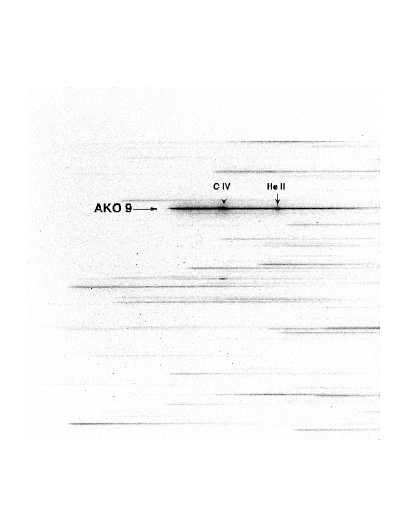
Figure 1:

Figure 2:

Figure 3:

Figure 4:

Figure 5:

Figure 6:

Figure 7:

Figure 8:

Figure 9:

Figure 10:

Figure 11:

References

- Albrow et al. (2001) Albrow, M. D., Gilliland, R. L., Brown, T. M., Edmonds, P. D., Guhathakurta, P., & Sarajedini, A. 2001, ApJ, 559, 1060
- (2) Auriére, M., Koch-Miramond, L., & Ortolani, S. 1989, A&A, 214, 113
- Bailyn et al. (1996) Bailyn, C. D., Rubenstein, E. P., Slavin, S. D., Cohn, H., Lugger, P., Cool, A. M., & Grindlay, J. E. 1996, ApJ, 473, L31
- Baptista et al. (1995) Baptista, R., Horne, K., Hilditch, R. W., Mason, K. O., & Drew, J. E. 1995, ApJ, 448, 395
- Baptista, Haswell, & Thomas (2002) Baptista, R., Haswell, C. A., & Thomas, G. 2002, MNRAS, 334, 198
- Bochkarev, Karitskaia, & Shakura (1979) Bochkarev, N. G., Karitskaia, E. A., & Shakura, N. I. 1979, AZh, 56, 16
- Campana et al. (1998) Campana, S., Colpi, M., Mereghetti, S., Stella, L., & Tavani, M. 1998, A&A Rev., 8, 279
- Chanan, Middleditch, & Nelson (1976) Chanan, G. A., Middleditch, J., & Nelson, J. E. 1976, ApJ, 208, 512
- (9) Cool, A. M., Grindlay, J. E., Cohn, H. N., Lugger, P. M. & Bailyn, C. D. 1998, ApJ, 508, L75
- Crampton, Fisher, & Cowley (1986) Crampton, D., Fisher, W. A., & Cowley, A. P. 1986, ApJ, 300, 788
- (11) Davies, M. 1997, MNRAS, 288, 117
- Dhillon, Marsh, & Jones (1991) Dhillon, V. S., Marsh, T. R., & Jones, D. H. P. 1991, MNRAS, 252, 342
- (13) Di Stefano, R. & Rappaport, S. 1994, ApJ, 423, 274
- Drew, Jones, & Woods (1993) Drew, J. E., Jones, D. H. P., & Woods, J. A. 1993, MNRAS, 260, 803
- Edmonds et al. (1996) Edmonds, P. D., Gilliland, R. L., Guhathakurta, P., Petro, L. D., Saha, A., & Shara, M. M. 1996, ApJ, 468, 241
- Edmonds et al. (2001) Edmonds, P. D., Gilliland, R. L., Heinke, C. O., Grindlay, J. E., & Camilo, F. 2001, ApJ, 557, L57
- Edmonds, Gilliland, Heinke, & Grindlay (2003) Edmonds, P. D., Gilliland, R. L., Heinke, C. O., & Grindlay, J. E. 2003, ApJ, in press (astro-ph/0307187)
- Eggleton (1983) Eggleton, P. P. 1983, ApJ, 268, 368
- (19) Fabian, A. C., Pringle, J. E., Rees, M. J. 1975, MNRAS, 172, L15
- Faulkner, Lin, & Papaloizou (1983) Faulkner, J., Lin, D. N. C., & Papaloizou, J. 1983, MNRAS, 205, 359
- Frank, King, & Raine (2002) Frank, J., King, A., & Raine, D. J. 2002, Accretion Power in Astrophysics, Cambridge University Press
- (22) Geffert, M., Auriére, M. & Koch-Miramond, L. 1997, A&A, 327, 137
- Gilliland (1982) Gilliland, R. L. 1982, ApJ, 263, 302
- Gilliland et al. (1995) Gilliland, R. L., Edmonds, P. D., Petro, L., Saha, A., & Shara, M. M. 1995, ApJ, 447, 191
- Gilliland et al. (2000) Gilliland, R. L. et al. 2000, ApJ, 545, L47
- Gratton et al. (2003) Gratton, R. G. et al. 2003, A&A, in press (astro-ph/0307016)
- Grindlay et al. (1995) Grindlay, J. E., Cool, A. M., Callanan, P. J., Bailyn, C. D., Cohn, H. N., & Lugger, P. M. 1995, ApJ, 455, L47
- (28) Grindlay, J. E., Heinke, C., Edmonds, P. D. & Murray, S. S. 2001a, Sci, 292, 2290
- (29) Grindlay, J. E., Heinke, C., Edmonds, P. D., Murray, S. S. & Cool, A. M, 2001b, ApJL, 563, 53
- (30) Hamada , T. & Salpeter, E. E. 1961, 134, 683
- Heinke et al. (2003) Heinke, C. O., Edmonds, P. D., Grindlay, J. E., Lloyd, D. A., Cohn, H. N., & Lugger, P. M. 2003, ApJ, 590, 809
- Hesser, Harris, & VandenBerg (1987) Hesser, J. E., Harris, W. E., & VandenBerg, D. A. 1987, PASP, 99, 1148
- Horne (1985) Horne, K. 1985, MNRAS, 213, 129
- Hut et al. (1992) Hut, P. et al. 1992, PASP, 104, 981
- King, Rolfe, & Schenker (2003) King, A. R., Rolfe, D. J., & Schenker, K. 2003, MNRAS, 341, L35
- Knigge, Woods, & Drew (1995) Knigge, C., Woods, J. A., & Drew, E. 1995, MNRAS, 273, 225
- Knigge & Drew (1997) Knigge, C. & Drew, J. E. 1997, ApJ, 486, 445
- (38) Knigge, C., Shara, M. M., Zurek, D. R., Long, K. S. & Gilliland, R. L. 2002, in: “Stellar Collisions, Mergers and their Consequences”, ed. M. M. Shara, ASP Conference Series, Vol. 263, p.137 (astro-ph/0012187)
- Knigge, Zurek, Shara, & Long (2002) Knigge, C., Zurek, D. R., Shara, M. M., & Long, K. S. 2002, ApJ, 579, 752 (Paper I)
- Kong et al. (2002) Kong, A. K. H., McClintock, J. E., Garcia, M. R., Murray, S. S., & Barret, D. 2002, ApJ, 570, 277
- Lucy (1967) Lucy, L. B. 1967, Zeitschrift für Astrophysik, 65, 89
- Minniti et al. (1997) Minniti, D., Meylan, G., Pryor, C., Phinney, E. S., Sams, B., & Tinney, C. G. 1997, ApJ, 474, L27
- Morris (1985) Morris, S. L. 1985, ApJ, 295, 143
- Paresce & de Marchi (1994) Paresce, F. & de Marchi, G. 1994, ApJ, 427, L33
- Pooley et al. (2002) Pooley, D. et al. 2002a, ApJ, 573, 184
- Pooley et al. (2002) Pooley, D. et al. 2002b, ApJ, 569, 405
- Popham & Narayan (1995) Popham, R. & Narayan, R. 1995, ApJ, 442, 337
- Pryor & Meylan (1993) Pryor, C. & Meylan, G. 1993, ASP Conf. Ser. 50: Structure and Dynamics of Globular Clusters, 357
- Russell (1945) Russell, H. N. 1945, ApJ, 102, 1
- Shara et al. (1996) Shara, M. M., Bergeron, L. E., Gilliland, R. L., Saha, A., & Petro, L. 1996, ApJ, 471, 804
- Thorstensen (2000) Thorstensen, J. R. 2000, PASP, 112, 1269
- (52) Tout, C. A., Pols, O. R., Eggleton, P. P. & Han, Z. 1996, MNRAS, 281, 257
- (53) VandenBerg, D. A. 2000, ApJS, 129, 315
- van Hamme (1993) van Hamme, W. 1993, AJ, 106, 2096
- Verbunt & Hasinger (1998) Verbunt, F. & Hasinger, G. 1998, A&A, 336, 895
- Warner (1995) Warner, B. 1995, “Cataclysmic Variable Stars”, Cambridge Astrophysics Series, Cambridge University Press
- Watson, King, & Osborne (1985) Watson, M. G., King, A. R., & Osborne, J. 1985, MNRAS, 212, 917
- Williger, Berriman, Wade, & Hassall (1988) Williger, G., Berriman, G., Wade, R. A., & Hassall, B. J. M. 1988, ApJ, 333, 277
- Wu et al. (1989) Wu, C., Holm, A. V., Panek, R. J., Raymond, J. C., Hartmann, L. W., & Swank, J. H. 1989, ApJ, 339, 443
- Yi & Kenyon (1997) Yi, I. & Kenyon, S. J. 1997, ApJ, 477, 379