GLOBAL ASYMPTOTIC SOLUTIONS FOR NON-RELATIVISTIC MHD JETS AND WINDS

Abstract

We present general and global analytical solutions, valid from pole to equator, for the asymptotic structure of non-relativistic, rotating, stationary, axisymmetric, polytropic, unconfined, perfect MHD winds. The standard five lagrangian first integrals along field lines are assumed known.

The asymptotic structure of such winds consists of field-regions virtually devoid of poloidal current. We show that an Hamilton-Jacobi equation, or equivalently a Grad-Shafranov equation, gives the asymptotic structure in the field regions. These field regions are bordered by current-carrying boundary layers around the polar axis and near null magnetic surfaces. Current closure is achieved in a number of separate cells bordered by null surfaces. The solution is given in the form of matched asymptotics separately valid outside and inside these boundary layers. The polar boundary layer is pressure-supported against the pinching force exerted by the axial poloidal current and has the structure of a current pinch, while the null-surface boundary layers have the structure of current sheet pinches. We establish a consistency relation between the residual poloidal current at large distances and the axial pressure. We find a similar relation for the current sheets at null surfaces. We further consider the case where the polar boundary layer is force free. The geometry of magnetic surfaces in all parts of the asymptotic domain is explicitly deduced in terms of the first-integrals.

The solutions have the following general properties:

I. For winds which are kinetic-energy dominated at infinity we derive WKBJ analytic solutions whose magnetic surfaces focus into paraboloids. The current slowly weakens as the inverse of the logarithm of the distance to the wind source while the axial plasma density falls-off as a negative power of this logarithm.

II. For winds carrying Poynting flux at large distances the solutions asymptotically approach to nested cylindrical and conical magnetic surfaces.

1 Introduction

We have previously established (Heyvaerts & Norman, 1989) that any stationary axisymmetric magnetized wind will collimate at large distances from the source, under perfect MHD conditions and polytropic thermodynamics, to paraboloids or cylinders along the symmetry axis according to whether the electric current (or Poynting flux) brought by the wind to infinity asymptotically vanishes or is finite. Our result however did not discriminate between these two possibilities, nor described any global asymptotic solution. The aim of this paper is to partially fill this gap. We consider here non-relativistic winds and concentrate on describing analytically their structure in the aymptotic region, for a supposedly given set of first integrals and for different, a priori possible, values of the circumpolar current at large distances.

We show here that the asymptotic structure of rotating MHD winds consists of vast regions where the poloidal current density is negligibly small, bounded by thin regions where residual asymptotic poloidal current flows. These regions have at large distances the character of boundary layers. They are located in the vicinity of the polar axis and of the null magnetic surfaces. We obtain solutions valid in all these regions separately and produce a global solution by asymptotic matching.

The specific topic which we are pursuing here is the construction of a general, non-self-similar, asymptotic solution globally valid from the polar axis to the equator, for a given set of supposedly known first integrals.

There has been in the past few years considerable progress in this field, both in the derivation of special exact solutions to the wind equation and in numerical solutions to them, both time dependent and stationary. Focusing of magnetized winds appears to be a robust property of rotating MHD winds (Blandford & Payne, 1982; Heyvaerts & Norman, 1989). Most analytical solutions involve some sort of self-similarity (Lovelace et al., 1991; Contopoulos & Lovelace, 1994; Ostriker, 1997; Trussoni et al., 1997; Vlahakis & Tsinganos, 1998, 1999). Lynden-Bell (1996) has constructed quasi-static, force-free collimated structures that arise naturally from a wound up magnetic field pushing out from a disk. The dynamics of such structures has been studied by Kudoh et al. (2002).

Sauty et al. (1992a, b), Sauty & Tsinganos (1994) and Sauty et al. (1999) have analytically considered particular models of non-polytropic winds and found that non-cylindrical asymptotics can be achieved only when magnetic pinching is negligible and there is over-pressure in the vicinity of the axis.

Shu and collaborators have extensively developed a X-wind model for outflows and in Shu et al. (1995) (plus references therein) they actually solved a Grad-Shafranov equation for the shape of the magnetic surfaces (Shafranov, 1996). They have an inner boundary condition of finite pressure. The launching region for T-Tauri winds has been examined recently by Anderson et al. (2003). Interesting disk instability can be initiated by wind driven angular momentum loss Cao & Spruit (2002). Tomisaka (2002) has found that the collapse of rotating magnetized molecular clouds and the resulting bipolar outflows are inextricably related.

Transfield force balance has also been studied by numerical simulations. These simulations studied hoop stresses collimation in different parameter regimes. Ustyugova et al. (1995) and Romanova et al. (1997) obtained two-dimensional solutions for jets emitted by a source with Keplerian rotation and confirmed the focusing effect of the hoop stress, as did Ouyed and Pudritz (1997a); Ouyed & Pudritz (1997b, 1999) who also found time-dependent behaviour. Lery & Frank (2000) found by two-dimensional simulation that winds orginating from a disk with a Keplerian rotation profile have a dense, current-carrying, central core surrounded by an almost current-free region. Ustyugova et al. (1999) numerically calculated this same problem using a model with a hot wind source region in the vicinity of the polar axis and found very little collimation within the simulation region. Ustyugova et al. (2000) studied formation of collimated Poynting jets associated with an uncollimated hydromagnetic outflow. Bogovalov & Tsinganos (1999) numerically found collimation to be most effective for a particular class of objects which they describe as ”efficient rotators”. In a subsequent paper Tsinganos & Bogovalov (2000) discussed the efficiency of collimation in the case of the solar wind. Boundary conditions at the base of the flow were found to be important. Bogovalov (1996, 2000) studied cold non-stationary flow from a monopole and found significant Poynting flux conversion to kinetic energy.

Since Heyvaerts & Norman (1989), papers similar in spirit to our own research have appeared. Li (1993) and Begelman & Li (1994) studied kinetic energy dominated winds and obtained asymptotic solutions that agreed with the paraboloidal solutions we had previously obtained. Tomimatsu (1995) constructed solutions in different regions including the pole and the equatorial null surface quite similar in spirit to the analysis presented here. Okamoto and collaborators (Okamoto, 1999, 2000; Beskin & Okamoto, 2000) emphasized the issue of current closure and its effect on the geometry of the solution. These issues which are, in fact, important only in boundary layers such as the equatorial current sheet, are now fully treated in this paper.

Our presentation is structured as follows. Section (2) reviews the basics of rotating MHD winds. Section (3) deals with the field-regions where almost no poloidal current flows. For Poynting jets the transfield equation becomes an Hamilton–Jacobi equation (Eq.(26)), or equivalently a Grad-Shafranov equation (Eq.(18)), which we solve in section (4) (Eq.(30)). Kinetic winds are solved using a WKBJ approximation. In section (5) we obtain the solution for the polar boundary layer (Eqs.(43)–(44)). This solution, which is similar to a Bennet pinch, is then matched to the field-region solution and a relation between the asymptotic current and the axial pressure is derived (Eq.(50)). The case of the force-free polar boundary layer is also discussed, giving a relation similar to the standard Bennet pinch (Eq.(70)). The matching procedure specifies the density along the polar axis (Eqs.(54)-(50)), the asymptotic circumpolar current and the radius of the current-carrying region (Eq.(57)). A slow logarithmic decline of the axial density and current is found in case of kinetic-energy-dominated winds, justifying the WKBJ approach. In section (6) we similarly obtain a solution valid in the vicinity of a null magnetic surface (Eqs.(76)–(79)) and match to the field-region solution. The gas pressure at the null surface balances the toroidal magnetic pressure outside the sheet (Eq.(102)). In section (7) the shape of the magnetic surfaces has been calculated in all regions and in both regimes. In the paraxial field-region of kinetic winds it is given by Eqs.(95)–(94). In the polar boundary layer it is given by Eq.(100). Inside an equatorial null-surface boundary layer of a kinetic wind it is given by Eq.(107), while inside the equatorial null-surface boundary layer of a Poynting jet it is given by Eq.(106). Our conclusions regarding the general properties of non-relativistic rotating MHD winds are presented in section (8).

2 Axisymmetric Stationary MHD Flows

2.1 Notation and Definitions.

The formulation of stationary axisymmetric rotating MHD winds have been presented in a number of papers (Weber & Davis, 1967; Okamoto, 1975; Mestel, 1999; Sakurai, 1985; Heyvaerts & Norman, 1989; Heyvaerts, 1996). Cylindrical coordinates $r$, $\theta$, $z$ are used with unit vectors $\vec{e}_{r}$, $\vec{e}_{\theta}$, $\vec{e}_{z}$. The spherical distance of a point to the origin is denoted by $R$. Vectors are split into toroidal and poloidal parts, indicated by subscripts $\theta$ and P respectively. The MKSA system of units is used with $\mu_{0}$ being the magnetic permeability of free space. The poloidal magnetic field can be expressed in terms of a magnetic flux function $a(r,z)$, such that

$$\vec{B}_{P}=-{1\over r}{\partial a\over\partial z}\ \vec{e}_{r}+{1\over r}{\partial a\over\partial r}\ \vec{e}_{z}.$$ (1)

The magnetic flux $\Phi_{m}$ through a circle of radius $r$ centered on the axis at altitude $z$ is $\Phi_{m}=2\pi a(r,z)$. The magnetic surfaces, generated by the rotation of field lines about the axis, are surfaces of constant value of $a(r,z)$. The value of $a$ labels magnetic surfaces or field lines.

2.2 First Integrals.

Mass conservation implies

$$\rho\vec{v}_{P}=\alpha(a)\vec{B}_{P},$$ (2)

where $\alpha(a)$ is a first integral. Flux freezing implies that

$$\rho v_{\theta}=\alpha(a)B_{\theta}+\rho r\Omega(a),$$ (3)

where $\Omega(a)$ is a second first integral. Conservation of specific angular momentum implies,

$$L(a)=rv_{\theta}-{rB_{\theta}\over{\mu_{0}\alpha(a)}}.$$ (4)

Conservation of the specific energy $E(a)$ implies:

$$E(a)={1\over 2}v_{P}^{2}+{1\over 2}v_{\theta}^{2}+{\gamma\over\gamma-1}{p\over\rho}+\Phi_{G}-{{rB_{\theta}\Omega(a)}\over{\mu_{0}\alpha(a)}}$$ (5)

$E(a)$ is the total specific energy carried by the wind on magnetic surface $a$, in kinetic and Poynting flux form. $\Phi_{G}$ is the gravitational potential. Equation (5) is the Bernoulli equation.

The thermodynamics is described by a lagrangian polytropic law, relating pressure and density, of the form

$$p=Q(a)\rho^{\gamma}$$ (6)

This defines a fifth first integral, $Q(a)$, the polytropic entropy. Equation (6) may represent adiabatic or more complex thermodynamics.

2.3 Semantics.

We define terms that will be used in this paper. The asymptotic domain consist of all points which are located on their own magnetic surface far away from the Alfvén point. A magnetic surface is said to be asymptotically parabolic if $r$ and $(z/r)$ both become infinite. This does not imply that $z$ should vary as a power law of $r$ at fixed $a$. A magnetic surface is said to be asymptotically conical if $r$ becomes infinite at large distances while $(z/r)$ approaches a finite limit $\tan\psi_{\infty}(a)$. This does not imply that $(z-r\tan\psi_{\infty})$ should approach a finite limit. Conical magnetic surfaces may have parabolic branches. An asymptotically cylindrical magnetic surface is one on which the axial distance $r$ approaches a finite limit $r_{\infty}(a)$.

When the asymptotic magnetic structure consists of cylindrical surfaces nested inside conical ones, the cylindrically focused one are refered to as forming the jet, and the other surfaces as forming the conical wind. The jet edge is defined as being the magnetic surface which separates asymptotically cylindrical from asymptotically conical surfaces. This terminology does not imply that only cylindrical asymptotics should give rise to structures that would appear to the observer as an astrophysical jet.

A neutral or null magnetic surface is one along which the poloidal field vanishes. The toroidal field then also vanishes on it. The immediate vicinity of neutral magnetic surfaces is of special interest, being regions where electric currents flow in the asymptotic domain. We refer to these regions as neutral surface boundary layers. Similarly, the vicinity of the polar axis is a region of electric current flow. We refer to it as the polar boundary layer. Outside the boundary layers is the field-region.

The space between two neighbouring neutral magnetic surfaces is refered to as a cell. The total electric current through a circle of axis $z$ passing through the point $(r,z)$ is:

$$J(r,z)=2\pi rB_{\theta}/\mu_{0}$$ (7)

$J$ vanishes at neutral surfaces and is negative for positive $\Omega$ and $\alpha$. Therefore we use the quantity

$$I=-{{rB_{\theta}}\over{\mu_{0}}}$$ (8)

which is positive for positive $\Omega$ and $\alpha$ and proportional to the current $J$. We refer to it as the current, noting that the true physical current is $J=-2\pi I$.

Strucures which convey a finite circumpolar electric current to infinity are refered to as Poynting jets. Kinetic winds carry no Poynting flux, or current, at infinity.

2.4 Bernoulli Equation

The toroidal components of the velocity and of the magnetic field can be obtained from the angular momentum conservation and isorotation law in terms of $\rho$ and $r$ as

$$v_{\theta}={L\over r}+{\rho\over r}\ {L-r^{2}\Omega\over\mu_{0}\alpha^{2}-\rho},$$ (9)

$$B_{\theta}={\mu_{0}\alpha\rho\over r}\ {L-r^{2}\Omega\over\mu_{0}\alpha^{2}-\rho}.$$ (10)

For well-behaved solutions the numerators must vanish when the denominators vanish. The cylindrical radius $r$ equals the Alfvén radius, $r_{A}(a)$, defined by $\Omega(a)\ r_{A}^{2}(a)=L(a)$, when the density $\rho$ equals the Alfvén density, $\rho_{A}(a)=\mu_{0}\alpha^{2}(a)$. The Alfvén radius defines the position of the Alfvén point on field line $a$. Asymptotically, for $r\gg r_{A}$, the azimuthal velocity vanishes while the variable $I=-rB_{\theta}/{\mu_{0}}$ approaches the value

$$I\rightarrow{{\rho r^{2}\Omega(a)}\over{\mu_{0}\alpha(a)}}$$ (11)

2.5 Transfield Equation

The projection of the equation of motion on the normal to the magnetic surfaces gives the transfield equation, or generalized Grad-Shafranov equation (eq. (A-1) of appendix A). It determines the shape of magnetic surfaces in terms of the first integrals and of the density. The set of coupled Bernoulli and transfield equations is to be solved. As shown in appendix A, the transfield equation can be reexpressed such as to give the curvature ($d\psi/ds$) of poloidal field lines in terms of various surface functions and of the current variable $I$. The resulting form of the transfield equation is:

$$\left(1-{\rho\over\rho_{A}}\right)v_{P}^{2}{d\psi\over ds}={{1}\over{\rho}}{\vec{\nabla}a\over|\nabla a|}\cdot\vec{\nabla}\left({{|\vec{\nabla}a|^{2}}\over{2\mu_{0}r^{2}}}+Q\rho^{\gamma}\right)+{\vec{\nabla}a\over|\nabla a|}\cdot\vec{\nabla}\Phi_{G}$$

$$-\left(L-I/\alpha\right)^{2}{1\over r^{3}}{\partial a/\partial r\over|\nabla a|}+{1\over\rho r^{2}}{\vec{\nabla}a\over|\nabla a|}\cdot\vec{\nabla}\left({\mu_{0}I^{2}\over 2}\right)$$ (12)

The terms on the right are the components of the poloidal magnetic pressure gradient, gas pressure gradient, gravity, centrifugal force and hoop stress respectively perpendicular to magnetic surfaces. The hoop stress is proportional to $\vec{j}_{P}\times\vec{B}_{\theta}$ and therefore vanishes with $I$.

3 Field Regions

3.1 Asymptotically Dominant Forces.

In the large-$z$ limit, Eq.(12) simplifies. The poloidal velocity $|v_{P}|$ reaches a terminal value and the curvature term on the left of equation (12) approaches zero. A definite ordering between the terms on the right of equation (12) occurs on magnetic surfaces on which both $z$ and $r$ tend to infinity. On asymptotically cylindrical magnetic surfaces, $r$ approaches a finite limit $r_{\infty}(a)$. However, when $r_{\infty}(a)\gg r_{A}(a)$ it still remains possible to use the large-$r$ approximation. In the large $r$, large $z$ and small $(\rho/\rho_{A})$ limit, noting that $\rho r^{2}$ is bounded from above (Heyvaerts & Norman, 1989) and that the gravity term declines as $1/r^{2}$ while the centrifugal force term declines as $1/r^{3}$, Eq.(12) reduces to:

$$v_{P}^{2}{d\psi\over ds}={r^{2}\Omega\over\mu_{0}\alpha I}{\vec{\nabla}a\over|\nabla a|}\cdot\vec{\nabla}\left({{\nabla a}^{2}\over 2\mu_{0}r^{2}}+Q\rho^{\gamma}\right)+{\Omega\over\alpha}{\vec{\nabla}a\over|\nabla a|}\cdot\vec{\nabla}I$$ (13)

When $I$ approaches a finite value, the hoop stress term, proportional to $\vec{n}\cdot\vec{\nabla}I$ decreases on conical magnetic surfaces as $(1/r)$ since $\vec{n}\cdot\vec{\nabla}I\approx I/r$. The hoop stress force then dominates all the other terms on the right of (13). The poloidal field $B_{P}$ decreases in this case as $(1/r^{2})$. The gradient of the poloidal magnetic pressure then drops with axial distance as $(1/r^{5})$, so that the corresponding term in Eq.(13) declines as $(1/r^{3})$. According to Eq.(2), the density decreases as $B_{P}$ when the velocity has reached its terminal value so that the gas pressure gradient scales as $(1/r^{2\gamma+1})$ and the pressure term in Eq.(13) declines as $(1/r^{2\gamma-1})$. This decline is slower than that of the poloidal magnetic pressure if the polytropic exponent $\gamma$ is less than 2, which we assume. The poloidal magnetic pressure is negligible compared to the gas pressure except in the ultra-cold limit where $Q$ vanishes. Therefore, we retain the gas pressure on the right of Eq.(13). The case of cold winds in which the poloidal magnetic pressure is retained is discussed in section (5.5).

Kinetic winds are characterized by $r|\vec{\nabla}a|$ and $\rho r^{2}$ approaching zero. The hoop stress scales as $\nabla I^{2}\sim\rho^{2}r^{3}$. The gas pressure gradient term scales as $\rho^{\gamma}/r$, and the poloidal magnetic pressure force $\sim\rho^{2}/r$. Again, gas pressure dominates over poloidal magnetic pressure, except for very cold winds. The hoop stress term dominates over the gas pressure force if $\rho^{2}r^{4}\gg\rho^{\gamma}$. This is so in the kinetic wind solutions derived below, since $\rho r^{2}$ is found to decline only as an inverse power of $(\ln r)$.

3.2 Transfield Equation

Neglecting pressure, the transfield equation (13) then further reduces to:

$$v_{P}^{2}{d\psi\over ds}=+{\Omega\over\alpha}{\vec{\nabla}a\over|\nabla a|}.\vec{\nabla}I$$ (14)

Eq.(14) is equivalent to Okamoto’s conclusion that $j_{\parallel}B_{t}=\rho v_{p}^{2}/R_{c}$, $R_{c}$ being the curvature radius of poloidal field lines (Okamoto, 1999). Note however that the centrifugal force associated with the poloidal field line curvature (on the left of equation (14)) is also negligible. Since the poloidal current is bounded from above, the right of equation (14) could a priori scale as $1/r$, but the curvature $(d\psi/ds)$ must decline with $r$ faster than $1/r$. Otherwise the poloidal field lines would not be well-behaved (Heyvaerts & Norman, 1989). The left of Eq.(14) is therefore of order $(v_{P}^{2}/R_{c})$ where $R_{c}$ is the curvature radius, much larger than $r$. To lowest order in the small parameter $(r/R_{c})$ Eq.(14) therefore reduces to the vanishing of its right-hand-side and becomes:

$$\vec{\nabla}a\cdot\vec{\nabla}I=0$$ (15)

This statement has been presented in Heyvaerts & Norman (1989) as a solvability condition at infinity. It implies that almost no poloidal electric current density is present in these regions.

3.3 Existence of Current Carrying Boundary Layers and Electric Circuit

Any physical current system must be closed. Current closure causes $I$ to depend on $a$ wherever current is flowing. This implies that some terms of Eq.(13) should balance hoop stress where current flows. Since this is not possible wherever $\nabla\approx 1/r$, this implies that regions of current flow must take the form of boundary layers in which gradients are large. Note that the hoop stress vanishes where the current vanishes. Boundary layers must then occur in the vicinity of the polar axis, where $B_{\theta}$ vanishes for finite current density at the axis, and near neutral surfaces, where the hoop stress vanishes with $B_{\theta}$. Indeed, the toroidal field component is generated from the poloidal one by the rotation, but the poloidal field vanishes at a neutral surface. In the case of a dipolar symmetry the equatorial plane is a neutral surface.

We then conclude that Eq.(15) applies in the field-region of the asymptotic domain, except in the boundary layers. Eq.(15) integrates along any trajectory orthogonal to magnetic surfaces as long as no null surface (in the vicinity of which equation (15) ceases to be valid) is met. The result is:

$$I=I_{\infty}(b)$$ (16)

where $b$ is a label for an orthogonal trajectory. To be specific, we define it as being the value of the $z$-coordinate on this orthogonal trajectory at the polar axis. An extra label, which we omit, should precise on which segment of the orthogonal trajectory Eq.(16) applies. Note that the magnetic surface label, $a$, and the orthogonal trajectory label, $b$, could constitute a set of orthogonal coordinates in the poloidal plane that could be substituted to $r$ and $z$, with $a$ playing the role of an angular variable and $b$ the role of a radial distance variable.

Eq.(15) states that the component of the poloidal current density parallel to $\vec{B}_{P}$ vanishes. Since $I_{\infty}(b)$ approaches a constant (possibly zero), so does also the other component of $\vec{j}_{P}$. Thus, the hoop stress $\vec{j}_{P}\times\vec{B}_{\theta}$, approaches zero, as does $\vec{j}_{\theta}\times\vec{B}_{P}$, since $|\vec{B}_{P}|$ declines rapidly with distance. Hence, the Lorentz force $\vec{j}\times\vec{B}$ approaches zero. This does not imply that the field becomes force free, because this decline is due to both current and field approaching zero. It is in fact quite interesting to analyze how the different components of the Lorentz force individually approach zero at large distance. This requires, however, a more precise knowledge of the solution than we have at this point. Therefore this discussion is postponed to appendix J. We emphasize that the asymptotic regime discussed in this paper is not force-free.

According to Eq.(16), the enclosed poloidal current is approximately constant through any circuit drawn on surfaces orthogonal to magnetic surfaces and running between two successive boundary layers. The current enclosed in a circle of increasing radius drawn on one such surface would increase from zero on the polar axis to some value at the outer edge of a polar boundary layer. The current remains almost constant up to the next null-surface, at which it returns to zero (Fig 1) through a boundary layer, vanishing at the null surface. Needless to say, Eqs.(15) and (16) are only approximate results. We do not mean that the current density is strictly zero in field regions, but only that it is so small that the total electric current circulating between two successive boundary layers through a surface of constant-$b$ is much less than the current in the boundary layers themselves. Nevertheless a small current in field regions must be present for $I_{\infty}$ to be a (slowly varying) function of $b$. This picture generalizes for any number of null surfaces and the current system consists of more than just two cells (Fig 2), in each of which the electric circuit separately closes. $I_{\infty}(b)$ approaching zero as $b\rightarrow\infty$ means that the poloidal current circuit closes in each cell at a finite distance. By contrast, $I_{\infty}(b)$ approaching a finite value, $I_{\infty}$, implies that this circuit would close at infinity. In reality, the wind has not been blowing for an infinite time and it is externally bordered by a time-dependent region and an expanding shock system. This region plays the role of the ”region at infinity” in the present stationary model: this is where the residual electric currents flow from the circumpolar region to the return-current boundary layers shown in Fig.(2).

Regions about the polar axis and the null surfaces must have the character of thin boundary layers since in the asymptotic domain, the gas pressure is a subdominant force that can balance Lorentz forces only in a small region about those special places where the latter vanishes. These boundary layer sheets must be thin and there must be toroidal magnetic pressure equilibrium accross them. The total poloidal current then only changes sign at their crossing as $\vec{B_{\theta}}$ reverses.

Our aim now is to solve the wind equations in the asymptotic domain, both in field-regions and in current-carrying boundary layers and obtain the resulting shape of the magnetic surfaces.

3.4 Asymptotic Grad-Shafranov Equation

From Eq.(14), it is possible to restate Eq.(15) as an equation similar to the familiar Grad-Shafranoff equation of magnetohydrostatics. Using the identity (A-2) of appendix A and Eqs.(11), (1) and (2), the equation (14) becomes:

$$r{{d\psi}\over{ds}}={{\mu_{0}I}\over{\Omega v_{\infty}}}\left({{r^{2}\Omega}\over{\mu_{0}I}}\ {\mathrm{div}}\left({{\Omega\vec{\nabla}a}\over{\mu_{0}I}}\right)-{{\partial}\over{\partial a}}\left({{v_{\infty}^{2}}\over{2}}\right)\right)$$ (17)

The above discussion indicates that the curvature radius should be much larger than r, so that the left of Eq.(17) is negligible. Expanding the divergence term and using Eqs.(2), (1) and (11) to express $r|\vec{\nabla}a|$, Eq.(17) is eventually brought to the form of a quasi-linear elliptic equation:

$$r^{2}\Delta a={{\partial}\over{\partial a}}\left({{\mu_{0}^{2}I^{2}v_{\infty}^{2}}\over{2\Omega^{2}}}\right)$$ (18)

The boundary conditions to Eq.(18) are that $a=0$ along the polar axis and that $a=A$ on the equatorial plane. These are consistent, when $I$ is constant and non-zero, with $a$ depending only on the latitude angle $\psi$. In this case Eq.(18) becomes an ordinary differential equation for $a(\psi)$, which reduces to the form of Eq.(33). Eq.(18) is equivalent to the other forms obtained above, in particular it implies Eq.(15). It is also equivalent to the alternative forms derived below, in particular Eq.(26). Using Eqs.(11), (1) and (2), an equivalent form of Eq.(18) is in fact found to be:

$$\Delta a=\vec{\nabla}a\cdot\vec{\nabla}\left(\ln\left(r|\vec{\nabla}a|\right)\right)$$ (19)

which can be brought by denoting the normal unit vector to poloidal field lines by $\vec{n}=-\vec{\nabla}a/|\vec{\nabla}a|$, to the form

$${\mathrm{div}}\left({{\vec{n}}\over{r}}\right)=0$$ (20)

4 Solutions in Field Regions

4.1 An Hamilton-Jacobi Equation

Noting that the velocity on each surface reaches a terminal velocity $v_{\infty}(a)$, Eqs. (2), (5) and (10) reduce in the asymptotic limit to:

$$\rho rv_{\infty}(a)=\alpha|\vec{\nabla}a|$$ (21)

$$I=+{{\rho r^{2}\Omega}\over{\mu_{0}\alpha}}$$ (22)

$$E={{v_{\infty}^{2}}\over{2}}+{{I\Omega}\over{\alpha}}$$ (23)

Eliminating $v_{\infty}$ and $\rho$ between Eqs.(21), (22) and (23), an expression of $r|\vec{\nabla}a|$ is obtained:

$$r|\vec{\nabla}a|={{\mu_{0}I\sqrt{2}\sqrt{\left(E-{{I\Omega}\over{\alpha}}\right)}}\over{\Omega}}$$ (24)

This relation can be integrated following orthogonal trajectories to magnetic surfaces. The curvilinear abcissa along them is denoted $\sigma$ and conventionally increases from pole to equator, so that $|\vec{\nabla}a|=da/d\sigma$. Eq.( 24) becomes

$${{d\sigma}\over{r}}=-{{\Omega(a)da}\over{\mu_{0}I(a,b)\sqrt{2}\sqrt{E(a)-I(a,b)\Omega(a)/\alpha(a)}}}$$ (25)

In field-regions, Eq. (25) simplifies, since $I(a,b)$ becomes a function $I_{\infty}(b)$ independent of $a$. It can be restated as:

$$r|\nabla a|={{\mu_{0}I_{\infty}(b)\sqrt{2}\sqrt{E(a)-I_{\infty}(b)\Omega(a)/\alpha(a)}}\over{\Omega(a)}}$$ (26)

If $I_{\infty}(b)$ were to approach a non-vanishing value $I_{\infty}$ at large distances from the wind source, this equation would explicitly give the flux distribution in space in the asymptotic domain. Particular versions of Eq.(26) for cylindrical or conical magnetic surfaces have in fact been obtained and solved in our earlier work (Heyvaerts & Norman, 1989). Eq. (26) improves on this by not being restricted to either one of these specific geometries. It implies no a priori constraints on the structure of the solution and keeps a fully 2-dimensional character. In the asymptotic field-region, far from the neutral surfaces and from the polar axis, the transfield equation reduces to Eq.(26) with constant $I_{\infty}(b)$, which is of the Hamilton-Jacobi type:

$$r|\nabla a|=f(a),$$ (27)

By defining $S(a)=\int_{0}^{a}{{da^{\prime}}/{f(a^{\prime})}}$, it can be converted into

$$|\nabla S|={1\over r},$$ (28)

This equation can be restated as $\vec{\nabla}S=-\vec{n}/r$, implying that $\vec{\nabla}\times(\vec{n}/r)=0$. This, with Eq.(20), indicates that $S$ should be an harmonic function. The solution for $S$ represented by Eq.(33) is harmonic.

If the poloidal electric current $I_{\infty}(b)$ declines towards zero at large distances, the function on the right of Eq.(27) also depends on $b$. Eq.(26) then does not provide the value of the modulus $|\nabla a|$ as a function of $a$ and $r$ (as does Eq.(27)) because it is not known how $I_{\infty}(b)$ declines with $b$. This difficulty can however be circumvented if this variation is so slow that it can be treated, as we do below, by a WKBJ type of approach. Note that the case when $I_{\infty}(b)$ approaches a non-zero limit, can be dealt with by a WKBJ procedure as well, since $I_{\infty}(b)$ is not strictly constant, but slowly evolves towards its limit. Important features of the asymptotic structure, in particular the difficult question of the connexion between the asymptotically cylindrical and the asymptotically conical regions, must be approached by considering the non-constancy of $I_{\infty}(b)$ as it approaches its limit.

Particular solutions to the Hamilton-Jacobi equation (27) for constant $I_{\infty}(b)$ can be found by the method of separation of variables. These are described in appendix D, although the boundary conditions associated to some of them are different from those we are facing. These solutions however exemplify a number of typical structures to which Eq.(27) may give rise. General solutions associated with the boundary conditions relevant to the case of astrophysical MHD winds can be found by reduction of Eq.(28) to a ray-tracing problem.

4.2 Ray-Tracing

Equation (28) is of the form $|\nabla S|=N(\vec{r})$, which is the Eikonal equation for the propagation of waves in a medium of index of refraction $N(\vec{r})$. The wave fronts are represented by surfaces of constant $S(\vec{r})$. They may be found by ray-tracing methods, the rays being the orthogonal trajectories to the surfaces. So, finding the general solution of Eq.(28) is equivalent to solving Snell’s refraction equation. We show in appendix (B) the equivalence of the Hamilton-Jacobi equation with Snell’s equation. The polar and the equatorial lines, being field lines, must be lines of constant $S$. The boundary condition to Eq.(28) is that rays start perpendicular to the pole and the equator. In the vicinity of a null surface (e.g. the equator), the simplified asymptotic transfield equation (15) is invalid. We show in section (7.5) and in appendix I that the angle of the magnetic field lines to the equator at the outskirts of this boundary layer decreases to zero with increasing $b$, justifying the view that rays from the field-region must nevertheless end perpendicular to it. Similar considerations apply to the vicinity of the pole and to other null surfaces: rays must also cross them perpendicularly on both sides.

This optical analogy can be used to find the general solution Eq.(28) by writing the appropriate form of Snell’s law. The gradient of the refraction index is in this case perpendicular to the polar axis. Let $i$ be the angle of incidence between this radial direction and the tangent to the ray. The ray-tracing equations can be written as:

$$dr=-d\sigma\ \cos i\qquad\qquad dz=d\sigma\ \sin i\qquad\qquad{{\sin i}\over{r}}=k$$ (29)

where $k$ is a constant. Unlike the boundary condition at the equator, the condition that $i$ approaches zero at the polar axis is not restrictive because $N(r)$, being equal to $1/r$, diverges there. Equations (29) can be integrated to:

$$(z-h)^{2}+r^{2}={{1}\over{k^{2}}}$$ (30)

where $h$ and $k$ are two integration constants. Eq.(30) represents a circle centered at $z=h$ on the axis, with a radius $D=1/k$. Lines of constant $S$ associated with the solution of equation (28) are orthogonal trajectories to a collection of circles centered on the polar axis. The boundary condition that the rays connect perpendicularly to the equator implies that $(h/D)$ should asymptotically vanish. It is important to note that this is not an exact, but only an approximate, asymptotic result. This is consistent with our earlier results (Heyvaerts & Norman, 1989). We show in appendix C that other conceivable current-enclosing geometries are not consistent with a source subtending a finite flux. We have assumed above that a unique cell extends from pole to equator. The extension to winds with a larger number of null surfaces is described in appendix E.

4.3 WKBJ Approximation

For $I_{\infty}(b)$ approaching a non-zero value as $b$ grows, the field-region of the flow consists of asymptotically conical magnetic surfaces in which current-carrying cylindrical ones are nested. When $I_{\infty}(b)$ approaches zero, we shall assume that it does so only very slowly, so that a WKBJ approach, which considers $I_{\infty}(b)$ as almost constant over large domains of $b$ values, will be possible. This approach assumes that the flux distribution on an orthogonal trajectory $b$ changes only very slowly when $b$ increases. The same WKBJ treatment can be used when $I_{\infty}(b)$ approaches a non-zero value, since it does so by only slowly varying. As explained before, considering this variation is a useful refinement. It is consistent to WKBJ analyze Eq.(15) without taking into account any of the other terms present in Eq.(13). The gas and poloidal magnetic pressure terms have been shown to be negligible to a certain order in $r^{-1}$. The relative order of magnitude of the inertia force associated to the curvature of the poloidal motion will define the order to which the WKBJ solution is consistent a posteriori. It will be shown that this term is indeed insignificant, even when compared to the gas pressure term, which is itself small in the field-region.

4.4 Solution in Field Regions

Orthogonal trajectories to magnetic surfaces are approximately circles centered at the origin. The distribution of flux on such a circle of radius $b$ can be represented by the distribution of latitude $\psi$ with flux $a$. In the WKBJ approximation, this distribution slowly changes from one circle to the next, so that $\psi$ depends not only on $a$ but also weakly on $b$, which we may now identify with the spherical distance $R$ since the orthogonal trajectory’s label in fact coincides with the distance to the origin all along it. Therefore, magnetic surfaces may be locally approximated by cones of semi-opening angle $(\pi/2-\psi(a,b))$. The equation for these cones is:

$$z=r\tan(\psi(a,b))$$ (31)

From this we obtain by differentiation and ignoring the WKBJ dependance on $b$:

$$|\nabla a|=-{cos\psi\over r\ \partial\psi/\partial a}$$ (32)

From Eq.(25) it results that $\psi(a)$ satisfies the differential equation:

$${{1}\over{\cos\psi}}\ {{d\psi}\over{da}}={{\Omega(a)}\over{\mu_{0}I(a,b)\sqrt{2}\sqrt{E(a)-I(a,b)\Omega(a)/\alpha(a)}}}$$ (33)

For this relation to give the flux distribution, the variation with $a$ of $I(a,b)$ must be known, which is the case only in field-regions of the asymptotic domain, where $I(a,b)$ becomes independent of $a$. In a current-carrying boundary layer $I(a,b)$ locally depends strongly on $a$ and should be determined by an analysis of the transfield equilibrium. In a field-region, where $I(a,b)$ reduces simply to $I_{\infty}(b)$, the solution of Eq.(33) is:

$$\tan(\psi(a,b))=\tan(\psi(a_{1},b))+\sinh\left(\int_{a}^{a_{1}}{{1}\over{\sqrt{2}\mu_{0}I_{\infty}(b)}}\ {{\Omega(a^{\prime})da^{\prime}}\over{\sqrt{E(a^{\prime})-I_{\infty}(b)\Omega(a^{\prime})/\alpha(a^{\prime})}}}\right)$$ (34)

where $a_{1}$ is a reference flux in the cell under consideration. If the cell begins at the equator, $a_{1}$ is the flux variable, $A$, for the equatorial surface and $\tan(\psi(A,b))=0$.

4.5 Flux Distribution in Cylindrical Regions of the Field.

In a region of the free field where the distribution of flux is cylindrical, orthogonal trajectories are better represented as straight lines perpendicular to the axis and Eq.(25) integrates to:

$$r_{\infty}(a)=r_{\infty}(a_{1})\exp\left(\int_{a_{1}}^{a}{{1}\over{\sqrt{2}\mu_{0}I_{\infty}}}\ {{\Omega(a^{\prime})da^{\prime}}\over{\sqrt{E(a^{\prime})-I_{\infty}\Omega(a^{\prime})/\alpha(a^{\prime})}}}\right)$$ (35)

where $a_{1}$ is a reference flux in the cylindrical field-region. The flux distribution described by Eqs.(34)-(35) with non-zero $I_{\infty}$ is represented, for arbitrarily chosen functions $\alpha$, $E$ and $\Omega$, in Fig.(6). A necessary, but not a sufficient, condition for such a solution to be obtained at very large distances from the source is that the function $(\alpha E/\Omega)$ has an absolute minimum. Whether a particular system, such as an accretion disk launching a centrifugal wind, can indeed meet this necessary condition can only be decided by solving the regularity conditions that this flow should satisfy. This point is addressed in the accompanying paper (Heyvaerts & Norman, 2002b), where we discuss whether the condition that $(\alpha E/\Omega)$ has a minimum value is sufficient to induce cylindrical collimation at infinity. We show that, in a purely mathematical sense, it is not but that in a physical sense it should be met in jets of a finite, albeit long, extent.

5 The Polar Boundary Layer

5.1 Solution in the Polar Boundary Layer.

The field-region solution does not apply to boundary layers. Within these boundary layers, the Lorentz force almost vanishes and forces that would elsewhere be negligible should be locally taken into account. The discussion of section (3.1) has shown that the pressure needs to be considered. In the case of pressureless winds, the poloidal magnetic pressure would be the dominant extra force. This situation is considered for completeness in section (5.5). Gravity declines to zero at large distances and the azimuthal velocity becomes very small at large $r/r_{A}$. Only if the ratio $r/r_{A}$ does not become very large would the centrifugal force play a role in the transfield equilibrium. In this section, we retain only gas pressure and hoop stress in our discussion of transfield equilibrium.

Physically, the polar boundary layer then locally has the structure of a column pinch. The asymptotic transfield equation can be written as Eq.(13), modified by using Eqs.(2) and (22), which first gives

$$v_{\infty}^{2}{{d\psi}\over{ds}}={{\Omega}\over{\alpha}}{{\vec{\nabla}a.\vec{\nabla}}\over{|\nabla a|}}\left({{\rho r^{2}\Omega}\over{\mu_{0}\alpha}}\right)+{{1}\over{\rho}}\ {{\vec{\nabla}a.\vec{\nabla}}\over{|\nabla a|}}\left(Q\rho^{\gamma}\right)$$ (36)

We find below that the axial density drops down with distance only very slowly, so that the poloidal curvature inertia term on the l.h.s. can also be neglected, being smaller than both the hoop stress and the pressure term. The transfield equation simplifies to:

$${\Omega\over\alpha}\ \vec{\nabla}a.\vec{\nabla}\left({{\rho r^{2}\Omega}\over{\mu_{0}\alpha}}\right)+{{1}\over{\rho}}\ \vec{\nabla}a\cdot\vec{\nabla}\left(Q\rho^{\gamma}\right)=0$$ (37)

Eq.(37) is readily integrated when the region of non-negligible pressure encompasses little enough flux that the first integrals $E$, $Q$, $\alpha$ and $\Omega$ can be treated as being constant in it, with values $E_{0}$, $Q_{0}$, $\alpha_{0}$, $\Omega_{0}$ say. In appendix F, we show this to be so when the asymptotic Poynting flux is small compared to the kinetic energy flux. If it is not, the pressure-supported region remains similar to a column-pinch, but its structure would now have to be calculated numerically. Assuming locally constant first integrals, then, equation (37) becomes

$$\vec{\nabla}a.\vec{\nabla}\left({{\rho r^{2}\Omega_{0}^{2}}\over{\mu_{0}\alpha_{0}^{2}}}+{{\gamma}\over{\gamma-1}}\ Q_{0}\rho^{\gamma-1}\right)=0$$ (38)

which integrates, following an orthogonal trajectory to magnetic surfaces, into:

$${{\rho r^{2}\Omega_{0}^{2}}\over{\mu_{0}\alpha_{0}^{2}}}+{{\gamma}\over{\gamma-1}}\ Q_{0}\rho^{\gamma-1}={{\gamma}\over{\gamma-1}}\ Q_{0}\rho_{0}^{\gamma-1}(b)$$ (39)

where $b$ is the radius of this quasi-circular orthogonal trajectory and $\rho_{0}(b)$ is the axial density at the distance $b$ from the source. Equation (39) can be solved for $r$ in terms of the parameter

$$x={{\rho}/{\rho_{0}}}$$ (40)

At the polar axis $x=1$ and far from it $x$ decreases to very mall values. Since $r=b\cos\psi$, this solution for $r(x)$ gives $\psi(x)$ at a given $b$, as expressed by Eq.(43). Close to the polar axis, the Bernoulli equation (5) reduces in the asymptotic domain to:

$${{v_{P}^{2}}\over{2}}=E_{0}-{{\gamma}\over{\gamma-1}}Q\rho_{0}^{\gamma-1}$$ (41)

The Poynting flux is negligible because $rB_{\theta}$ vanishes proportionally to $r^{2}$. On the other hand, $|\vec{v}_{P}|$ is related to $|\vec{\nabla}a|$ by Eqs.(1) and (2). With the approximation of a constant $\alpha(a)$ in the polar boundary layer, this gives, using Eq.(32):

$$|\vec{v}_{P}|={{\alpha_{0}}\over{b^{2}\rho_{0}(b)}}{{da/dx}\over{x\ \cos\psi\ (d\psi/dx)}}$$ (42)

By using Eq.(43) for $\psi(x)$, Eqs.(41) and (42), a simple differential equation for $a(x)$ is obtained, which is valid for $(\pi/2-\psi)\ll 1$. Its solution is given by Eq.(44). This provides the following parametric representation of the solution very near the polar axis:

$$cos^{2}\psi={{\gamma Q_{0}\rho_{0}^{\gamma-2}(b)\ \mu_{0}\alpha_{0}^{2}}\over{(\gamma-1)\ \Omega_{0}^{2}b^{2}}}\left({{1}\over{x}}-{{1}\over{x^{2-\gamma}}}\right)$$ (43)

$$a={{\gamma\ Q_{0}\rho_{0}^{\gamma-1}(b)\ \mu_{0}\alpha_{0}}\over{\sqrt{2}(\gamma-1)\ \Omega_{0}^{2}}}\sqrt{E_{0}-{{\gamma}\over{\gamma-1}}Q_{0}\rho_{0}^{\gamma-1}(b)}\ \left(\ln{{{1}\over{x}}}-{{2-\gamma}\over{\gamma-1}}\left(1-x^{\gamma-1}\right)\right)$$ (44)

5.2 Matching the Polar Boundary Layer Solution to the Outer Solution.

Eliminating $x$, when small (which corresponds to the outer regions of the polar boundary layer) between equations (43) and (44) gives the relation between $a$ and $\psi$ valid in these intermediate regions:

$$\cos^{2}\psi={{\gamma}\over{\gamma-1}}\ {{Q_{0}\mu_{0}\alpha_{0}^{2}\rho_{0}^{\gamma-2}(b)}\over{\Omega_{0}^{2}\ b^{2}}}\ \exp\left(a\ \ {{(\gamma-1)\ \sqrt{2}\ \Omega_{0}^{2}}\over{\gamma\ Q_{0}\rho_{0}^{\gamma-1}(b)\mu_{0}\alpha_{0}\sqrt{E_{0}-{{\gamma}\over{\gamma-1}}Q_{0}\rho_{0}^{\gamma-1}(b)}}}\right)$$ (45)

It can be asymptotically matched to the outer solution (34). In the vicinity of the polar axis, $\tan\psi$ is large, and the constant term $\tan\psi(a_{1})$ can be neglected if the reference magnetic surface $a_{1}$ is not one of cylindrical geometry. The relation (34) can be expressed as:

$$\cos\psi=\left(\cosh\chi\right)^{-1}$$ (46)

where

$$\chi(a,b)={{1}\over{\sqrt{2}\mu_{0}I_{\infty}(b)}}\int_{a}^{a_{1}}{{\Omega(a^{\prime})da^{\prime}}\over{\sqrt{E(a^{\prime})-I_{\infty}(b)\Omega(a^{\prime})/\alpha(a^{\prime})}}}$$ (47)

Near the polar axis $\chi$ is large and approximately given by

$$\chi(a,b)\approx{{1}\over{\sqrt{2}\mu_{0}I_{\infty}(b)}}\left(\int_{0}^{a_{1}}{{\Omega(a^{\prime})da^{\prime}}\over{\sqrt{E(a^{\prime})-I_{\infty}(b)\Omega(a^{\prime})/\alpha(a^{\prime})}}}-{{\Omega_{0}\ a}\over{\sqrt{E_{0}-I_{\infty}(b)\Omega_{0}/\alpha_{0}}}}\right)$$ (48)

which, by Eq.(46), gives the inner limit of the outer solution as:

$$\cos^{2}\psi=4\ \ \exp\left(-\ \ {{\sqrt{2}}\over{\mu_{0}I_{\infty}(b)}}\left[\int_{0}^{a_{1}}{{\Omega(a^{\prime})da^{\prime}}\over{\sqrt{E(a^{\prime})-I_{\infty}(b)\Omega(a^{\prime})/\alpha(a^{\prime})}}}-{{\Omega_{0}\ a}\over{\sqrt{E_{0}-I_{\infty}(b)\Omega_{0}/\alpha_{0}}}}\right]\right)$$ (49)

5.3 Bennet Pinch Relation

For the exponential arguments in Eqs.(45) and (49) to coincide, it is necessary that:

$${{\gamma}\over{\gamma-1}}\ Q_{0}\rho_{0}^{\gamma-1}(b)={{I_{\infty}(b)\ \Omega_{0}}\over{\alpha_{0}}}$$ (50)

Eq.(50) expresses a relation between the total current supported by the polar boundary layer and its inner pressure. The existence of a relation between the total current and the central pressure is common to all cylindrical plasma pinches and is usually refered to as a Bennet relation.

5.4 Polar Boundary Layer Current, Density and Radius

For smooth asymptotic matching, the factors in front of the exponential functions in Eqs.(45) and (49) must coincide. Taking Eq.(50) into account, this condition can be written as:

$${{\gamma Q_{0}\ \mu_{0}\alpha_{0}^{2}\rho_{0}^{\gamma-2}(b)}\over{(\gamma-1)b^{2}\Omega_{0}^{2}}}=4\ \ \exp\left(-\ {{\sqrt{2}(\gamma-1)\ \Omega_{0}}\over{\gamma\ \mu_{0}\alpha_{0}\ Q_{0}\rho_{0}^{\gamma-1}(b)\ }}\ \int_{0}^{a_{1}}{{\Omega(a^{\prime})\ da^{\prime}}\over{\sqrt{E(a^{\prime})-I_{\infty}(b)\Omega(a^{\prime})/\alpha(a^{\prime})}}}\right)$$ (51)

It can be more conveniently written by defining a length $\ell$, a dimensionless measure of the density, $n_{0}(b)$, and a reference magnetic flux $a_{0}$ by:

$$\ell^{2}={{\gamma}\over{(\gamma-1)}}\ {{Q_{0}\rho_{A0}^{\gamma-1}}\over{\Omega_{0}^{2}}}\qquad\qquad\qquad n_{0}(b)=\rho_{0}(b)/\rho_{A0}\qquad\qquad\qquad a_{0}={1\over 2}\ \mu_{0}\alpha_{0}\sqrt{2E_{0}}\ \ell^{2}$$ (52)

and by using the notation

$$\lambda=\int_{0}^{a_{1}}{{\Omega(a^{\prime})\ \sqrt{E_{0}}}\over{\Omega_{0}\ \sqrt{E(a^{\prime})-I_{\infty}(b)\Omega(a^{\prime})/\alpha(a^{\prime})}}}\ {{da^{\prime}}\over{a_{0}}}$$ (53)

The integral $\lambda$ depends on $\rho_{0}(b)$, or $n_{0}(b)$, because of Eq.(50). The logarithm of Eq.(51) then takes the form:

$${{\lambda(n_{0}(b))}\over{n_{0}^{\gamma-1}(b)}}=(2-\gamma)\ \ln(n_{0}(b))\ +\ \ln\left({{4b^{2}}\over{\ell^{2}}}\right)$$ (54)

Since $n_{0}(b)$ is small and ($b/\ell$) large, an approximate solution can be obtained by iteration, initially neglecting the $\ln\left(n_{0}\right)$ term on the r.h.s. as compared to $n_{0}^{-(\gamma-1)}$ on the l.h.s.. This gives at the simplest degree of approximation:

$$n_{0}^{\gamma-1}(b)={{\lambda(b)}\over{2\ln\left({{2b}\over{\ell}}\right)}}$$ (55)

Eqs.(54) and (55) are dominated by the growth of the logarithm term on their r.h.s. They can be satisfied for large $b$’s in two different ways, according to whether the current $I_{\infty}(b)$ at the boundary layer’s edge approaches a finite value or decreases to zero.

When $I_{\infty}(b)$ approaches a finite value, the Bennet relation (50) shows that the axial density should be independent of distance. The logarithmic term in the denominator of equation (55) should then be compensated by a divergence of the numerator term $\lambda(b)$ (Eq.(53)). This shows that, as $b$ increases, $I_{\infty}(b)$ should approach a limit that causes the integral on the r.h.s. of Eq.(53) to diverge. This implies that the asymptotic limit of $I_{\infty}(b)$ be the absolute minimum of the function $(\alpha E/\Omega)$, which, given the presence of a square root denominator in the integral on the r.h.s. of Eq.(53), can only be approached from below. Therefore $I_{\infty}(b)$ should in this case asymptotically grow towards the absolute minimum of $(\alpha E/\Omega)$.

If $I_{\infty}(b)$ declines asymptotically to zero, the function $\lambda(b)$ approaches a limit independent of $b$. This indicates that equation (55) should be satisfied by the decrease of $n_{0}(b)$ to zero at large distances. This is consistent with the fact that in this case all the magnetic surfaces flare out parabolically (Heyvaerts & Norman, 1989) Equation (55) implies a specific law of decrease of $\rho_{0}(b)$, namely, denoting the limit of $\lambda(b)$ for zero current by $\lambda_{0}$:

$$\rho_{0}(b)\approx\mu_{0}\alpha_{0}^{2}\left({{\lambda_{0}}\over{2\ln\left({{2b}\over{\ell}}\right)}}\right)^{{{1}\over{\gamma-1}}}$$ (56)

It is then seen that $\rho_{0}(b)$ scales with $b$ as $\left({\ln({{b}/{\ell}}})\right)^{-{{1}\over{\gamma-1}}}$. The residual current $I_{\infty}(b)$, given by equation (50), slowly decreases as $\left({\ln({{2b}/{\ell}}})\right)^{-1}$.

The radius $r_{0}$ of the circumpolar current channel at distance $b$ is the value of $r=b\ \cos\psi$ given by Eq.(43) for some intermediate value, of order unity, of the parameter $x$. This gives

$$r_{0}^{2}={{\gamma Q_{0}\rho_{0}^{\gamma-2}(b)\ \mu_{0}\alpha_{0}^{2}}\over{(\gamma-1)\ \Omega_{0}^{2}}}$$ (57)

For Poynting jets, this expression gives the specific value of this radius, since $\rho_{0}$ is given by Eq.(50). For kinetic winds, the boundary layer radius slowly increases with distance $b$ as $\left(\ln(b/\ell)\right)^{{{(2-\gamma)}\over{2(\gamma-1)}}}$.

At this point the solution near the pole and in the field region extending in the polar-most cell is completely determined. In particular, the solution for the flux distribution in the field-region of this cell can, by using Eqs.(49), (51) and (47), be expressed as

$$b^{2}\cos^{2}\psi={{\gamma Q_{0}\ \mu_{0}\alpha_{0}^{2}\rho_{0}^{\gamma-2}(b)}\over{(\gamma-1)\Omega_{0}^{2}}}\ \ \exp\left({{\sqrt{2}}\over{\mu_{0}I_{\infty}(b)}}\int_{0}^{a}{{\Omega(a^{\prime})da^{\prime}}\over{\sqrt{E(a^{\prime})-I_{\infty}(b)\Omega(a^{\prime})/\alpha(a^{\prime})}}}\right)$$ (58)

and $\rho_{0}$ and $I_{\infty}$ are related by Eq.(50).

5.5 Force-Free Polar Boundary Layers

If the poloidal magnetic pressure dominates plasma pressure, the corresponding cylindrical structure is described by the transfield mechanical balance equation (13):

$${r^{2}\Omega\over\mu_{0}\alpha I}{\vec{\nabla}a\over|\nabla a|}\cdot\vec{\nabla}\left({{\nabla a}^{2}\over 2\mu_{0}r^{2}}\right)+{\Omega\over\alpha}{\vec{\nabla}a\over|\nabla a|}\cdot\vec{\nabla}I=0$$ (59)

This equation should be associated with the cylindrical asymptotic form of Eq.(5)

$$E(a)={{v_{P}^{2}}\over{2}}-{{r\Omega B_{\theta}}\over{\mu_{0}\alpha}},$$ (60)

with the mass conservation equation (2), with Eq.(11) and with Eq.(1). The latter reduces in this geometry to

$$B_{P}={1\over r}\ {{da}\over{dr}}$$ (61)

The variables $v_{P}$ and $\rho$ can be eliminated by Eqs.(2) and (11) in favour of the field component $B_{P}$ and the quantity $I$. Using Eq.(60), $B_{P}$ can then also be expressed in terms of $I$. We are left, for given $b$, with a pair of ordinary differential equations for $I(r)$ and $a(r)$ where the first integrals, which are known functions of $a$, also appear. This system is

$${{d}\over{dr}}\left({{\mu_{0}I^{2}}\over{r^{4}\Omega^{2}}}\ \left(E-{{I\Omega}\over{\alpha}}\right)\right)+{{\mu_{0}}\over{r^{2}}}\ {{d}\over{dr}}\left({{I^{2}}\over{2}}\right)=0$$ (62)

$${{1}\over{r}}\ {{da}\over{dr}}={{\sqrt{2}\mu_{0}I}\over{r^{2}\Omega}}\sqrt{E-{{I\Omega}\over{\alpha}}}$$ (63)

As in the case of pressure-supported polar boundary layers, we assume that the first integrals do not vary much over the current carrying boundary layer and treat them as being constants, $\alpha_{0}$, $E_{0}$ and $\Omega_{0}$ say. This is valid for ${\Omega I}/{\alpha E}\ll 1$ (app.F) and allows to transform Eq.(62) to the simpler form:

$${{E_{0}}\over{\Omega_{0}^{2}}}\ {{d}\over{dr}}\left({{I^{2}}\over{r^{4}}}\right)+{{1}\over{r^{2}}}\ {{d}\over{dr}}\left({{I^{2}}\over{2}}\right)=0$$ (64)

This shows that the natural unit length $r_{0}$ in the force free pinch, or in other words the core radius of this pinch, is:

$$r_{0}^{2}={{E_{0}}\over{\Omega_{0}^{2}}}$$ (65)

This relation replaces equation (57) for pressure-supported axial boundary layers. The solution of equation (64) is

$$I(r,b)=I_{\infty}(b)\ {{\Omega_{0}^{2}r^{2}}\over{\Omega_{0}^{2}r^{2}+2E_{0}}}$$ (66)

The solution (66) can be asymptotically matched with the field-region solution (34). Actually the solution (66) itself explicitly shows this continuuous transition from $I=0$ to $I=I_{\infty}$. It establishes the relation, which replaces Eq.(50), between the total electric current carried by the polar boundary layer and the poloidal magnetic pressure that supports the associated pinching force. The poloidal field and plasma density can be expressed from Eqs.(2) and (11) in terms of $I$ as:

$${{B_{P0}^{2}(b)}\over{\mu_{0}}}={{2\mu_{0}E_{0}}\over{\Omega_{0}^{2}}}\ \lim_{r\rightarrow 0}\left({{I^{2}}\over{r^{4}}}\right)$$ (67)

and

$$\rho_{0}(b)={{\mu_{0}\alpha_{0}}\over{\Omega_{0}}}\ \lim_{r\rightarrow 0}\left({{I}\over{r^{2}}}\right)$$ (68)

The limiting value involved is obtained from Eq.(66):

$$\lim_{r\rightarrow 0}\left({{I}\over{r^{2}}}\right)={{I_{\infty}\Omega_{0}^{2}}\over{2E_{0}}}$$ (69)

Equations (67), (68), (69) can be synthesized in the relation:

$${{B_{P0}^{2}(b)}\over{\mu_{0}\rho_{0}(b)}}={{I_{\infty}(b)\Omega_{0}}\over{\alpha_{0}}}$$ (70)

which is the form of Bennet pinch relation appropriate to this case. It differs from Eq.(50) only by the substitution of the axial Alfvén speed to the axial sound speed.

6 Null Surface Boundary Layers

6.1 Divergence of the Mass Flux to Magnetic Flux Ratio at Null Surfaces

At a null surface, labelled by $a_{n}$ say, the mass flux to magnetic flux ratio, $\alpha(a)$, defined by Eq.(2), diverges as $a\rightarrow a_{n}$ if there is mass flux on this null surface. We show in appendix (G) that the divergence of $\alpha(a)$ is as

$$\alpha(a)\sim{{1}\over{|a_{n}-a|^{\nu}}}$$ (71)

where $\nu$ is a positive number stricly less than unity. Usually, $\nu=1/2$.

6.2 Structure of Null Surface Boundary Layers.

The structure of the flow near a null-surface can be derived from the transfield equation (13). The ratio of the gas pressure to the toroidal magnetic pressure decreasing to zero as the axial distance $r$ increases, the thickness of the pressure-dominated region about the null surface, $\eta$, becomes small at large distances. The gradient operator normal to the magnetic surface, $\vec{\nabla}a\cdot\vec{\nabla}/|\nabla a|$, noted as $-\vec{n}\cdot\vec{\nabla}$, is then of order $\eta^{-1}$ when acting on $I$ or on $Q\rho^{\gamma}$. The left hand side of equation (13) being smaller than ($v_{P}^{2}/r$) (see section (3.1)), can thus be neglected. Similarly the variable $r$ can be treated as a constant because ($\vec{n}\cdot\vec{\nabla}r$), of order unity, is negligible to ($r/\eta$). Eq.(13) then reduces, using Eq.(8), to:

$$\vec{n}\cdot\vec{\nabla}\left(Q\rho^{\gamma}+{{B_{\theta}^{2}}\over{2\mu_{0}}}\right)=0$$ (72)

which, by using Eq.(11) and regarding $Q$ and $\Omega$ as constants, $Q_{n}$ and $\Omega_{n}$, takes the form

$$\vec{n}\cdot\vec{\nabla}\left(Q_{n}\rho^{\gamma}+{1\over 2}\ {{\rho^{2}r^{2}\Omega_{n}^{2}}\over{\mu_{0}\alpha^{2}}}\right)=0$$ (73)

Since $\alpha$ diverges at a null surface (section 6.1 and app. G) this integrates as

$$Q_{n}\rho^{\gamma}+{1\over 2}\ {{\rho^{2}r^{2}\Omega_{n}^{2}}\over{\mu_{0}\alpha^{2}}}=Q_{n}\rho_{n}^{\gamma}(r)$$ (74)

where $\rho_{n}(r)$ is the density at the cylindrical distance $r$ of the axis on this null surface. Let us introduce the parameter

$$X=\rho/\rho_{n}(r)$$ (75)

The mass to flux ratio $\alpha(a)$ is given in terms of $X$ by Eq.(74), namely:

$${{1}\over{\mu_{0}\alpha^{2}(a)}}={{2Q_{n}\rho_{n}^{\gamma-2}(r)}\over{\Omega_{n}^{2}r^{2}}}\left({{1}\over{X^{2}}}-{{1}\over{X^{2-\gamma}}}\right)$$ (76)

Note that, as it should, $\alpha^{-1}$ vanishes as the neutral surface is approached, when $X$ approaches unity. When the functional dependence of $\alpha(a)$ on $a$ is known, Eq.(76) gives $a$ in terms of $X$. Since this dependence is however not universal (see Eq.(71)), this step cannot be performed in a general way. Close to a neutral surface, the Bernoulli equation (5) reduces, in the asymptotic domain, to :

$$E={{v_{P}^{2}}\over{2}}+{{\gamma}\over{\gamma-1}}Q\rho^{\gamma-1}-{{r\Omega B_{\theta}}\over{\mu_{0}\alpha}}$$ (77)

where $B_{\theta}$ can be obtained from Eq.(11). Using Eq.(76) to account for the variation of $\alpha(a)$ in the neighborhood of the neutral surface, we obtain, using Eq.(75) and neglecting the variations of $r$ accross the boundary layer,

$${{v_{P}^{2}}\over{2}}\approx E_{n}-{{2-\gamma}\over{\gamma-1}}Q_{n}\rho_{n}^{\gamma-1}X^{\gamma-1}-2Q_{n}\rho_{n}^{\gamma-1}X^{-1}$$ (78)

On the other hand, $|\vec{v}_{P}|$ is related to $|\vec{\nabla}a|$ by Eqs.(1) and (2). Using Eq.(32), this provides a differential equation for the dependance of the latitude angle $\psi$ on $a$, or equivalently, on $X$, at a given $b$. Using Eq.(78) this differential equation can be written as:

$$b\ d\psi=-{{\alpha(a)da}\over{\sqrt{2}\ rX\rho_{n}\ \sqrt{E-{{2-\gamma}\over{\gamma-1}}Q_{n}\rho_{n}^{\gamma-1}X^{\gamma-1}-2Q_{n}\rho_{n}^{\gamma-1}X^{-1}}}}$$ (79)

Eq.(79) could be brought to quadratures for $\psi(X)$ if the explicit dependance of $a$ on $X$ could be deduced from Eq.(76) for known, and invertible, $\alpha(a)$, such as for example in Eq.(71). This step will not be taken here explicitly because the relation between $a$ and $\alpha$ does not have an universal character, even near a neutral layer. Although we have not derived the solution explicitly, we can still proceed to deduce the necessary conditions for a smooth matching to the solution in the far field.

6.3 Matching the Null Surface Boundary Layer Solution to the Field

The solution in the boundary layer about the neutral surface is now given by equations (76) and (79). It can be asymptotically matched to the field-region solution which is expressed in differential form by equation (33). In the field-region near the neutral surface Eq.(33) reduces to:

$$d\psi=-{{\Omega_{n}da}\over{\mu_{0}I_{\infty}(b)\sqrt{2}\sqrt{E_{n}-I_{\infty}(b)\Omega_{n}/\alpha(a)}}}$$ (80)

On the other hand, eliminating $X$ between Eqs.(76) and (79) in the small $X$ limit, which is relevant to the outskirts of the equatorial boundary layer, we obtain a differential equation for $\psi$ valid in this region:

$$d\psi=-{{\Omega_{n}da}\over{r\sqrt{2}\sqrt{2\mu_{0}Q_{n}\rho_{n}^{\gamma}(r)}\sqrt{E_{n}-{{\Omega_{n}}\over{\mu_{0}\alpha}}\sqrt{2\mu_{0}Q_{n}r^{2}\rho_{n}^{\gamma}(r)}}}}$$ (81)

Matching requires that equations (80) and (81) be identical. This implies that the total current at the edge of the null surface boundary layer at a distance $b$ from the wind source (corresponding to an axial distance $r$) is related to the density at the center of the layer by:

$$\mu_{0}I_{\infty}(r)=\sqrt{2\mu_{0}Q_{n}r^{2}\rho_{n}^{\gamma}(r)}$$ (82)

This relation expresses the balance between gas pressure at the null surface and the magnetic pressure just at the outer edge of its boundary layer, as expected for a sheet-pinch. As a result we find that, for Poynting jets, the equatorial density decreases as

$$\rho_{n}(r)\sim r^{-{2\over\gamma}}$$ (83)

For kinetic winds, $I_{\infty}(r)$ decreases as $1/(\ln\left(2r/\ell\cos\psi_{n})\right))$ and the density at the null magnetic surfaces declines as:

$$\rho_{n}(r)\sim\left(r\ \ln\left({{2r}\over{\ell\cos\psi_{n}}}\right)\right)^{-{2\over\gamma}}$$ (84)

6.4 Flux and Current Distribution Near a Neutral Surface.

Eq.(33) indicates that $(d\psi/da)$ becomes infinite at a neutral magnetic surface, where $I$ vanishes. Does that imply that $\tan\psi$ becomes infinite at neutral surfaces? In a given current cell, Eq.(33) integrates similarly to Eq.(34) to:

$$\tan(\psi(a,b))=\tan(\psi(a_{1},b))+\sinh\left(\int_{a}^{a_{1}}{{1}\over{\sqrt{2}\mu_{0}I(a^{\prime},b)}}\ {{\Omega(a^{\prime})da^{\prime}}\over{\sqrt{E(a^{\prime})-I(a^{\prime},b)\Omega(a^{\prime})/\alpha(a^{\prime})}}}\right)$$ (85)

Whether $tan(\psi)$ diverges or not as $a$ approaches $a_{n}$ depends on the behaviour of the integral on the r.h.s. of Eq.(85) as the neutral surface is approached and this in turn depends on how $I(a,b)$ varies with $(a-a_{n})$ as the neutral surface $a_{n}$ is approached. This can be deduced from the solution expressed by Eq.(76). The current $I$ in the asymptotic domain is given by Eq.(22). Using Eqs.(75) and (76) it is found that:

$$I^{2}\approx{{2Q_{n}r^{2}\rho_{n}^{\gamma}(r)}\over{\mu_{0}}}\left(1-X^{\gamma}\right)$$ (86)

The parameter $X$ is related to $\alpha$, or $(a-a_{n})$, by Eq.(76). It is shown in section (6.1) that $\alpha$ scales with $(a_{n}-a)$ as:

$$\alpha^{-1}\sim(a_{n}-a)^{\nu}$$ (87)

where $\nu$ is a positive exponent strictly smaller than unity, usually equal to ${1\over 2}$. Very near the neutral surface, $X$ is close to unity. From Eq.(76), it is found that:

$$(a-a_{n})^{2\nu}\sim{{2Q_{n}\rho_{n}^{\gamma-2}}\over{\Omega_{n}r^{2}X^{2}}}\left(1-X^{\gamma}\right)$$ (88)

Comparing this with Eq.(86), we conclude that, very near the null surface,

$$I\sim(1-X^{\gamma})^{1/2}\sim(a-a_{n})^{\nu}$$ (89)

With such a dependence of $I$ on $a$ the integral in Eq.(85) converges as $a$ approaches $a_{n}$, since $\nu$ is less than unity. Therefore, neutral surfaces do not become vertical when approached from a conical region.

7 Shape of the Magnetic Surfaces

We have now obtained a complete solution in the asymptotic domain, both in field-regions (section (4.4)) near the pole (section (5.1)) and near neutral magnetic surfaces (section (6.2)). Since the integral in Eq.(85) converges at a neutral surface, integration may be started at the equator, irrespective of whether or not it is a neutral surface. At the equator, $\tan\psi$ vanishes, and thus the integration constant of Eqs.(34) and (85) can be taken to be zero. The solution is then extended to other angles $\psi$ by using either Eq.(85) or appropriate solutions in the neutral or polar boundary layers to specify how $I(a,b)$ depends on $a$ at given $b$.

The dependence of $I_{\infty}(b)$ on $b$ in field-regions is determined by solving Eq.(54), $\lambda(b)$ being defined by Eq.(53) and $I_{\infty}$ by Eq.(50). Eq.(54) may have one or two solutions at large $b$, depending on the function $(\alpha E/\Omega)$.

We now have gathered all the information needed to calculate the asymptotic shape of magnetic surfaces, both in the field-region and in the various boundary layers.

7.1 Magnetic Surfaces in Field-regions of Poynting Jets

When the flow is a Poynting jet, its magnetic structure consists of cylindrical surfaces nested into conical ones. The relation between flux and radius for cylindrical surfaces is given by equations (43) and (44) in the polar boundary layer, noting that $r\equiv b\cos\psi$, and by (58) and (50) outside of it. The dependence of the latitude angle of conical magnetic surfaces on flux is given by (34) in the field-region. When there is only one cell extending from pole to equator, $a_{1}$ can be taken as the equatorial flux $A$ and $\tan\psi(a_{1})$ reduces to zero, since there is vanishing flux left in the equatorial boundary layer at large distances. The shape of the magnetic surfaces in the equatorial boundary layer itself is obtained in section 7.4.

7.2 Magnetic Surfaces in Field-regions of Kinetic Winds

The magnetic surfaces of kinetic winds are described by Eq.(34), $I_{\infty}(b)$ being now given by the analysis of section (5.4) (Eqs.(54)-(55)). By Eq.(50) we get, for small $I_{\infty}(b)$:

$$\mu_{0}I_{\infty}(b)=\left(\int_{0}^{A}{{\Omega(a)da}\over{\sqrt{2E(a)}}}\right)\ \ {{1}\over{\ln\left({{b}\over{l}}\right)}}$$ (90)

We consider the case of polar and equatorial boundary layers of kinetic winds in sections 7.3 and 7.4 respectively. In the field-regions the shape of magnetic surfaces is given by the solution of the following differential equations for $r(b)$ and $z(b)$:

$$dr=\cos\psi(a,b)\ \ db\qquad\qquad dz=\sin\psi(a,b)\ \ db$$ (91)

which are to be integrated in $b$ for constant $a$. The latter argument will be omitted below. The angle $\psi(a,b)$ is given by Eqs.(46)-(47). Since magnetic surfaces are in this case parabolic, $\psi$ is close to $\pi/2$ and the spherical distance $b$ can be identified with $z$. Eq.(91) then reduces to

$$dr=\cos\psi(z)\ dz$$ (92)

Similarly, Eq.(46) for $\psi$ simplifies, for large $\chi$’s and for $I_{\infty}(b)$ as given by eq. (90), to:

$$\cos\psi(z)=\ 2\left({{\ell}\over{2z}}\right)^{k(a)}$$ (93)

where $k(a)$ is:

$$k(a)={{\int_{a}^{A}{{\Omega(a^{\prime})\ da^{\prime}}\over{\sqrt{E(a^{\prime})}}}}\over{\int_{0}^{A}{{\Omega(a^{\prime})da^{\prime}}\over{\sqrt{E(a^{\prime})}}}}}$$ (94)

Noting $q(a)=1-k(a)$, the solution of Eq.(92) is:

$${{r}\over{\ell}}={{1}\over{q(a)}}\left({{2z}\over{\ell}}\right)^{q(a)}$$ (95)

The magnetic surfaces are then, in the paraxial region outside of the polar boundary layer, a collection of nested power-law paraboloids of variable exponent. Some sections of the magnetic surfaces, though extending out of the equatorial boundary layer, may still be close enough to the equator that the paraxial approximation $\psi\approx\pi/2$, is inappropriate for them. Their shape should be found by integrating Eqs.(91) with no further approximation, as done in appendix H.

7.3 Magnetic Surfaces in the Polar Boundary Layer

In the polar boundary layer of Poynting jets, magnetic surfaces are cylinders. For kinetic winds, the paraxial approximation is fully justified in this region and the shape of magnetic surfaces is given by Eqs.(43)-(44), with the notations of Eqs.(52). Eq.(43) can be written as:

$${{r^{2}}\over{\ell^{2}}}={{1}\over{n_{0}^{2-\gamma}(b)}}\left({{1}\over{x}}-{{1}\over{x^{2-\gamma}}}\right)$$ (96)

whith Eq.(44) providing the value of the parameter $x$ in terms of $a$ by:

$$\ln{{1}\over{x}}-{{2-\gamma}\over{\gamma-1}}\left({1-x^{\gamma-1}}\right)={{a}\over{a_{0}}}\ {{1}\over{n_{0}^{\gamma-1}(b)}}$$ (97)

The dimensionless axial density $n_{0}(b)$ is approximately given by Eq.(55). The spherical distance to the origin being almost identical to $z$, Eqs.(96)-(97) constitute a set of coupled equations relating $x$, $r$ and $z$. With the notations of Eqs. (52)-(53) they can be written as:

$${{r^{2}}\over{\ell^{2}}}=\left({{1}\over{x}}-{{1}\over{x^{2-\gamma}}}\right)\left(2{{\ln\ ({{2z}/{\ell}})}\over{\lambda}}\right)^{{2-\gamma}\over{\gamma-1}}$$ (98)

$$\left({{2a}\over{\lambda a_{0}}}\right)\ \ln\left({{2z}\over{\ell}}\right)=\left(\ln{{1}\over{x}}-{{2-\gamma}\over{\gamma-1}}\left(1-x^{\gamma-1}\right)\right)$$ (99)

This system can be solved to give $r$ and $z$ in terms of $x$. For small $x$ we recover the paraxial field-region solution, while for $x$ close to unity we obtain the shape of magnetic surfaces in the pressure-dominated region very near the polar axis. In this region the magnetic surfaces switch from algebraic paraboloids to exponential ones, their shape being given by:

$${{r}\over{\ell}}=\sqrt{{{a}\over{a_{0}}}}\ \left({2\over\lambda}\right)^{{1}\over{2(\gamma-1)}}\ \left({\ln\ {{2z}\over{\ell}}}\right)^{{1}\over{2(\gamma-1)}}$$ (100)

7.4 Magnetic Surfaces in the Equatorial Boundary Layer

Let us assume for simplicity that the only neutral surface is the equatorial plane. The information on the shape of magnetic surfaces in its boundary layer is provided by the parametric solution of Eqs.(76) and (79). The density in the equatorial plane at the distance $r\equiv b$ from the source, $\rho_{e}(b)$, is related to the polar residual current $I_{\infty}(b)$ by Eq.(82). $I_{\infty}(b)$ approaches a constant value for Poynting jets and decreases logarithmically for kinetic winds. Both cases can be unified by writing

$$I_{\infty}(b)={{J_{m}}\over{\left(\ln(2b/\ell)\right)^{m}}}$$ (101)

where $m=0$ for Poynting jets and $m=1$ for kinetic winds, the factor $J_{m}$ being different in the two cases. Equation (82) then gives for the equatorial density

$$\rho_{e}(b)=\left({{\mu_{0}J_{m}^{2}}\over{2Q_{e}}}\right)^{1/\gamma}\ \left({{1}\over{b\ (\ln(2b/\ell))^{m}}}\right)^{2/\gamma}$$ (102)

For small $X$ we recover from Eqs. (76) and (79) the results valid in the field-region. Eliminating $\alpha$ from Eq.(79) and using Eqs.(76) and (82) we get:

$$z=b\ \int_{a}^{A}{{\Omega_{e}\ da}\over{\sqrt{2\mu_{0}Q_{e}b^{2}\rho_{e}^{\gamma}(b)}\ \ \sqrt{2\ (E_{e}-I_{\infty}(b)\Omega_{e}/\alpha)}}}$$ (103)

When $I_{\infty}$ approaches a non-vanishing constant so does, from Eq.(82), $b^{2}\rho_{e}^{\gamma}(b)$. Then $z/b$ approaches, at fixed $a$, a constant value: the magnetic surfaces become conical at the outskirts of the equatorial boundary layer, as they should. For kinetic winds, Eq.(103) gives, considering Eq.(101):

$$z\approx{{\Omega_{e}(A-a)}\over{J_{0}\sqrt{2E_{e}}}}\ \ b\ln\left({{2b}\over{\ell}}\right)$$ (104)

and the magnetic surfaces become slightly convex paraboloids at the outskirts of the equatorial boundary layer. By contrast, in the region of the equatorial boundary layer where the gas pressure dominates, $X$ is close to unity and the integration of Eqs.(76) and (79) gives:

$$z=\int_{a}^{A}{{\alpha(a)da}\over{b\ \rho_{e}(b)}}{{1}\over{\sqrt{2\left(E_{e}-{{\gamma}\over{\gamma-1}}\ Q_{e}\rho_{e}^{\gamma-1}(b)\right)}}}$$ (105)

where again $\rho_{e}(b)$ is given by Eq.(102). It is then found that $z(b)$ scales, at fixed $a$, as

$$z\sim b^{{{2-\gamma}\over{\gamma}}}$$ (106)

for Poynting jets and as

$$z\sim b^{{{2-\gamma}\over{\gamma}}}\ \left(\ln\left({{2b}\over{\ell}}\right)\right)^{2\over\gamma}$$ (107)

for kinetic winds. Note that in this region magnetic surfaces are concave and bend towards the equator. This agrees with the conclusions of Okamoto (1999), although the force balance considered by this author is between the Lorentz force and the poloidal curvature inertia force, whereas we consider balance between the Lorentz force and the pressure gradient force. This does not contradict the results of Heyvaerts & Norman (1989) because this is by no means the terminal shape of these magnetic surfaces. Indeed, as discussed in section 7.5 below and in Appendix I, any magnetic field line eventually escapes the equatorial boundary layer region, first joining a region at its outskirts where its shape becomes conical or parabolic as indicated by Eq.(103) and eventually reaching the field-region.

7.5 Exit from the Equatorial Boundary Layer

When magnetic surfaces exit the equatorial boundary layer, they do so with an angle to the equatorial plane that decreases with distance. The discussion of section (4.2) assumed trajectories orthogonal to magnetic surfaces to cross normal to the equator. For dipolar symmetry, an equatorial boundary layer is always present between the field-region and the equator itself. The boundary conditions used in section (4.2) are thus consistent only if the latitude angle of field lines at the outer edge of the equatorial boundary layer becomes increasingly negligible with distance. We show in appendix I that the slope $(\partial z/\partial b)$ of the exiting field line indeed decreases to zero with distance along the equatorial boundary layer.

7.6 Justification of WKBJ Treatment

Our WKBJ treatment of the field-region solution is valid only if the inertia force associated with the curvature of the poloidal motion remains negligible. In the case of Poynting jets, the poloidal field lines in the field-region asymptotically become exactly straight so that solving Eq.(13), supposedly valid to order $r_{A}/r$, while ignoring the curvature term at the l.h.s. of Eq.(12) is obviously consistent. In the case of kinetic winds, the poloidal field lines are described by Eqs.(H-5)-(H-6) of appendix H, where their radius of curvature has also been calculated. This radius is proportional to $(r^{{{1+k}\over{1-k}}}/k)$ on field lines for which the exponent defined by Eq.(94) is $k$. Since $k$ approaches unity at the pole, the neglect of the force due to poloidal curvature is fully justified in these regions. Near the equator, where $k$ approches zero, the curvature radius comes closer to scaling as $r$, but remains still much larger than $r$. This is because $k$ never reduces exactly to zero and because of the presence of the dividing factor $k$, which reflects the fact that when field lines become tangent to the equator, their curvature must be very small.

8 Conclusions

We have derived global solutions for the asymptotic structure of non-relativistic, rotating, stationary, axisymmetric, polytropic, unconfined, perfect MHD winds. The five lagrangian first integrals are assumed to be known.

The asymptotic structures have been found to consist of vast regions, called field regions, which are devoid of any significant residual poloidal electric current density. Residual current flows in thin regions in the vicinity of the polar axis and the neighbourhood of null magnetic surfaces. Null surfaces can occur at polarity reversals of the wind source or extend over dead zones. They delineate separate cells in which the poloidal current achieves closure.

For kinetic-energy-dominated winds the conversion of total wind energy to kinetic energy is shown to progress only logarithmically with distance.

All winds have been shown to possess a circumpolar current-carrying boundary layer, which has the structure of a pressure-supported plasma-jet pinch. Null-surface boundary layers have the structure of pressure-supported current sheets. The total electric current is constant or slowly diminishes with distance according to an inverse logarithmic law for the Poynting flux and kinetic winds respectively. This dimunition is caused by minute amounts of current flowing through the diffuse field regions from the pole to the nearest null surface.

The pressure in the center of these regions, where the toroidal field vanishes, is related to the residual current by Bennet pinch relations. The plasma density remains constant at the polar axis or declines as a negative power of the logarithm of the distance to the wind source as above. Therefore, Poynting flux can be retained, even in kinetic winds, over large distances.

We have calculated the structure of the flow in all possible regions including field regions, the polar boundary layer and null-surface boundary layers. The solution is given in terms of standard first-integrals using a WKBJ approximation that incorporates the weak dependence on the distance from the source. A complete solution has been constructed by asymptotic matching of these separate pieces of the solution. Global relations are found between the circumpolar current and the density at the polar axis or at neutral surfaces (Eqs.(50) and (82)). We have established similar relations in the case of jets with force free polar boundary layers (Eq.(70)).

The shapes of magnetic surfaces in all parts of the solution and in all relevant regimes have been calculated as well. The results are as follows:

I. For winds which are kinetic-energy dominated at infinity:

(i) In the free field, the magnetic surfaces focus into algebraic paraboloids (Eq.(95)) as shown in Fig.3.

(ii) In the polar boundary layer, the magnetic surfaces focus into exponential paraboloids (Eq.(100)) as shown in Fig.4.

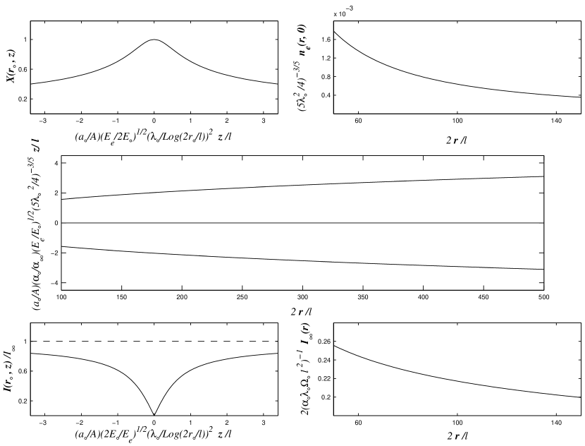
Figure 5: The behavior of kinetic winds about the equatorial boundary layer. The panels show: the magnetic field structure (central); the normalized density $n_{e}$ = $\frac{\rho(r,0)}{\rho_{A0}}$ in the equatorial plane vs. distance along the equatorial plane (upper right); the total current integrated about the equatorial plane vs. distance along the equatorial plane (lower right); the ratio of the density to its equatorial value at the same $r$ across the equatorial sheet (upper left) and the integrated current across the equatorial sheet (lower left). The latter two quantities are plotted for some arbitrary value of $r$, $r_{0}$. For simplicity, $\Omega_{e}$, $\alpha_{e}$ and $Q_{e}$ have been set equal to $\Omega_{0}$, $\alpha_{0}$ and $Q_{0}$ respectively. The field lines (central frame, Eq.(107)) correspond to $\frac{a}{A}$ = 0.9. Their parabolic shape is not clearly visible on the scale of the plot. The plots in the right panels are from Eqs.(82) and (84), while those in the left panels are from Eqs.(75), (76), (86) and (87) with $\nu$ = $\frac{1}{2}$. For these plots, the adiabatic index $\gamma$ has been taken to be equal to $\frac{4}{3}$.

(iii) Near a null surface, which could be the equatorial plane, the lines are concave, bending towards the equator deep inside the neutral boundary layer (Eq.(107)). The magnetic surfaces become straight lines with a logarithmic correction (Eq.(104)) at the edge of the layer. These lines are convex, bending away from the equatorial plane, outside the neutral sheet as shown in Fig.5.

II. For winds carrying Poynting flux at infinity:

(i) In the free field the solutions asymptote to nested cylindrical and conical magnetic surfaces. (Eqs.(35) and (34)) as shown in Fig.6.

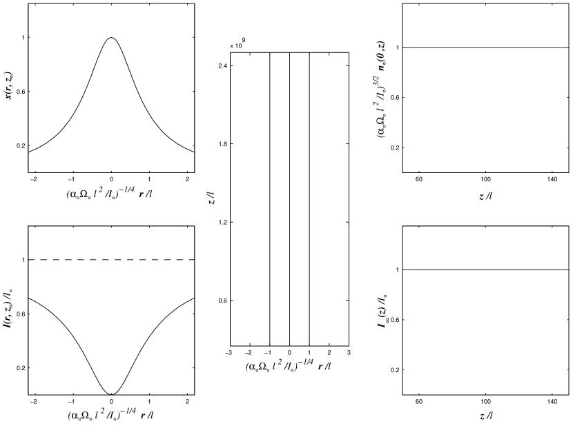
Figure 7: The behaviour of Poynting jets near the polar axis. The plots show: magnetic field structure (central frame); the normalized density at the polar axis vs. the distance along the polar axis (upper right); the total current integrated about the polar axis vs. the distance along the polar axis (lower right); the ratio of the density to its polar value at the same $z$ across the polar pinch (upper left) and the integrated current across the polar axis (lower left). The latter two quantities are plotted for some arbitrarily chosen $z_{0}$. The central frame shows that the field lines are exact cylinders (Eq.(57)). The right panel curves use Eqs.(50) and (52). The left panel curves are obtained from Eqs.(40), (43), (44), (22) and (52). $I_{0}$ here is the absolute minimum of $\frac{\alpha E}{\Omega}$.

(ii) In the polar boundary layer they are cylindrical (Eqs.(43)–(44)) as shown in Fig.7.

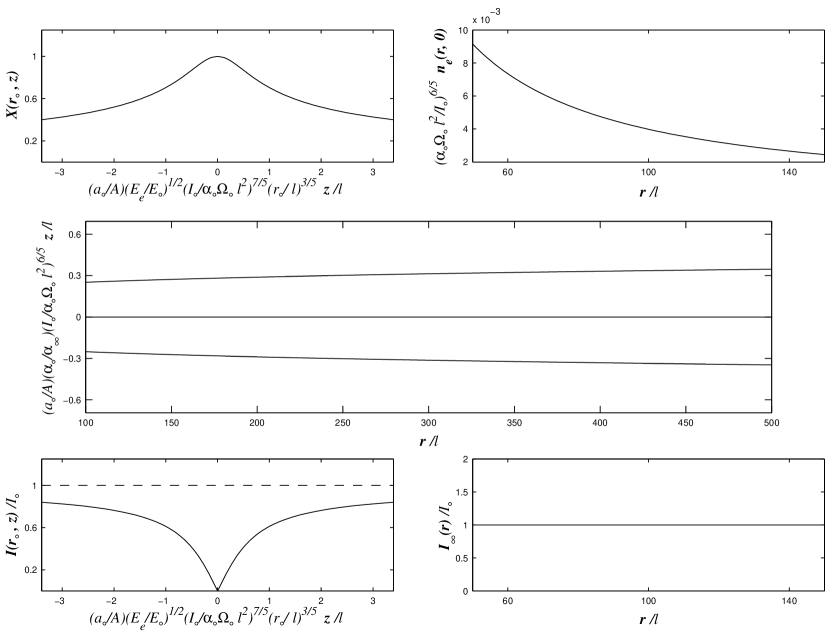
Figure 8: The behaviour of Poynting jets about the equatorial boundary layer. The plots show: magnetic field structure (central frame, from Eq.(106)); the normalized density $n_{e}$ = $\frac{\rho(r,0)}{\rho_{A0}}$ in the equatorial plane vs. distance along the equatorial plane (upper right); the total current integrated about the equatorial plane vs. distance along the equatorial plane (lower right); the ratio of the density to its equatorial value at the same $r$ across the equatorial sheet (upper left) and the integrated current across the equatorial sheet (lower left). The latter two quantities are plotted for some arbitrary value of $r$, $r_{0}$. The field structure (central frame) is plotted for $\frac{a}{A}$ = 0.9. The plots in the right panels are from Eqs.(82) and (83), while those in the left panels are from Eqs.(75), (76), (86) and (87) with $\nu$ = $\frac{1}{2}$. For these plots, the adiabatic index $\gamma$ has been taken to be equal to $\frac{4}{3}$.

(iii) Near a null surface, which could be the equatorial plane, the lines are concave, bending towards the equator deep inside the neutral boundary layer (Eq.(106)). The magnetic surfaces become straight lines (Eq.(103)) at the edge of the layer. These lines remain straight outside the neutral sheet as shown in Fig. 8.

From an observational point of view, the polar and null surface boundary layers which carry residual electric current may stand out against the field-regions, both because of their large density contrast and because they are a source of free energy. This free energy (associated with the currents) has the potential of making them active, by the development of instabilities. The density about the pole does not decline with distance in the case of Poynting jets, or does it only very slowly in the case of kinetic winds. It may be that what is observed as a jet is the dense and active polar boundary layer of a flow developped on a much larger angular scale. On these larger scales the flow may be difficult to observe because of its very low density and current. Null-surface boundary layers, for example equatorial ones, could be observed in association with the jets, although their density and activity is expected to decline more rapidly with distance than on the polar axis, because of geometrical effects. Their detection could be misinterpreted as accretion disks.

The conclusions reached in this paper are of course only valid under our assumptions of stationnarity, axisymmetry, polytropic thermodynamics, perfect MHD and unconfinement. None of those is expected to be exactly satisfied in reality. Nevertheless we believe that the electric circuit picture which emerges from our analysis should be robust against relaxing a number of these assumptions. Our description of current closure must remain a feature of the solution, because current leakage between main regions of current flow should remain weak when the large regions between them suffer little instability. This is expected to be the case for regions devoid of current and with only small velocity gradients. Forces competing with hoop stress must also remain small under rather general conditions and are probably confined to spatially limited regions. By contrast, the distribution of flux in the different boundary layers would be modified by the consideration of non-ideal effects, such as turbulence resulting from the development of non axisymmetric MHD instabilities. The stationnarity assumption is valid on a scale smaller than the size of the cavity carved by the wind in the ambient medium. The wind is bordered by a time dependent region featuring an expanding shock system. Actually this region is where the residual electric currents flow from the circum-polar region to the return regions. That the system, on a scale less than that of the global cavity, reaches stationarity seems to be a reasonable assumption.

In the following paper (Heyvaerts & Norman, 2002a) we generalize these results to the relativistic regime. An additional paper (Heyvaerts & Norman, 2002b) discusses whether magnetized outflows are kinetic-energy-dominated or carry Poynting flux.

Appendix A Curvature of Poloidal Field Lines

We write the projection of the equation of motion on the normal to the magnetic surfaces as (see for example Heyvaerts & Norman (1989)):

$${\alpha\over\rho r}\left[{\partial\over\partial z}{\alpha\over\rho r}{\partial a\over\partial z}+{\partial\over\partial r}{\alpha\over\rho r}{\partial a\over\partial r}\right]-{1\over\mu_{0}\rho r}\left[{\partial\over\partial z}{1\over r}{\partial a\over\partial z}+{\partial\over\partial r}{1\over r}{\partial a\over\partial r}\right]=E^{\prime}(a)-{Q^{\prime}(a)\over\gamma-1}\rho^{\gamma-1}$$

$$+{\alpha^{\prime}\over\alpha}{\mu_{0}\alpha^{2}\rho\over r^{2}}\left({L-r^{2}\Omega\over\mu_{0}\alpha^{2}-\rho}\right)^{2}-{\rho\over r^{2}}(L^{\prime}-r^{2}\Omega^{\prime})\left({L-r^{2}\Omega\over\mu_{0}\alpha^{2}-\rho}\right)-{LL^{\prime}\over r^{2}}.$$ (A-1)

where primed quantities are derivatives with respect to $a$ of surface functions. The transfield equation (A-1) can be transformed by making use of the following relations which can be derived by explicit calculation of $({\rm{curl}}\ \vec{v}_{P}\times\vec{v}_{P})$ and $({\rm{curl}}\ \vec{B}_{P}\times\vec{B}_{P})$, using also Eq.(2):

$${\alpha\over\rho r}\left[{\partial\over\partial z}{\alpha\over\rho r}{\partial a\over\partial z}+{\partial\over\partial r}{\alpha\over\rho r}{\partial a\over\partial r}\right]=-{{\vec{\nabla}a}\over{|\nabla a|^{2}}}\left((\vec{v}_{P}\cdot\vec{\nabla})\vec{v}_{P}-\vec{\nabla}({v_{P}^{2}\over 2})\right)$$ (A-2)

$${1\over r}\left[{\partial\over\partial z}{1\over r}{\partial a\over\partial z}+{\partial\over\partial r}{1\over r}{\partial a\over\partial r}\right]=-{{\vec{\nabla}a}\over{|\nabla a|^{2}}}\left((\vec{B}_{P}\cdot\vec{\nabla})\vec{B}_{P}-\vec{\nabla}({B_{P}^{2}\over 2})\right)$$ (A-3)

The vectors $\vec{v}_{P}$ and $\vec{B}_{P}$ are separated in modulus and direction as $\vec{v}_{P}=v_{P}\ \vec{t}$ and $\vec{B}_{P}=B_{P}\ \vec{t}$, with $\vec{t}$ the unit vector tangent to the poloidal field line. This gives:

$$(\vec{v}_{P}\cdot\vec{\nabla})\vec{v}_{P}=v_{P}^{2}\ (\vec{t}\cdot\vec{\nabla})\vec{t}+\vec{t}\ (\vec{t}\cdot\vec{\nabla})(v_{P}^{2}/2)$$ (A-4)

and a similar equation for $\vec{B}_{P}$. Then use is made of the Fresnet formula $(\vec{t}\cdot\vec{\nabla})\vec{t}=\vec{n}(d\psi/ds)$ whith $\psi$ the angle between the vector $\vec{t}$ and its projection onto the equatorial plane, $s$ the curvilinear abcissa along the poloidal field line and $\vec{n}$ the unit normal vector oriented towards the polar axis ($\vec{n}=-{\vec{\nabla a}/|\nabla a|}$). This transforms equations (A-2) and (A-3) into

$${\alpha\over\rho r}\left[{\partial\over\partial z}{\alpha\over\rho r}{\partial a\over\partial z}+{\partial\over\partial r}{\alpha\over\rho r}{\partial a\over\partial r}\right]={v_{P}^{2}\over|\nabla a|}{d\psi\over ds}-{\vec{n}\over|\nabla a|}\cdot\nabla({v_{P}^{2}\over 2})$$ (A-5)

$${1\over r}\left[{\partial\over\partial z}{1\over r}{\partial a\over\partial z}+{\partial\over\partial r}{1\over r}{\partial a\over\partial r}\right]={B_{P}^{2}\over|\nabla a|}{d\psi\over ds}-{\vec{n}\over|\nabla a|}\cdot\nabla({B_{P}^{2}\over 2})$$ (A-6)

The transfield equation (A-1) is thus reduced to the form:

$${v_{P}^{2}\over|\nabla a|}(1-{\rho\over\rho_{A}}){d\psi\over ds}={\vec{n}\cdot\vec{\nabla}\over|\nabla a|}\left({v_{P}^{2}\over 2}\right)-{1\over\mu_{0}\rho}{\vec{n}\cdot\vec{\nabla}\over|\nabla a|}\left({B_{P}^{2}\over 2}\right)$$

$$+E^{\prime}-{Q^{\prime}\rho^{\gamma-1}\over\gamma-1}+{\alpha^{\prime}\over\alpha}{\rho_{A}\rho\over r^{2}}\left({L-r^{2}\Omega\over\rho_{A}-\rho}\right)^{2}-{\rho\over r^{2}}{(L^{\prime}-r^{2}\Omega^{\prime})(L-r^{2}\Omega)\over\rho_{A}-\rho}-{LL^{\prime}\over r^{2}}$$ (A-7)

Eliminating $v_{P}^{2}/2$ on its r.h.s. by Eq.(5), Eq.(A-7) becomes:

$${v_{P}^{2}\over|\nabla a|}(1-{\rho\over\rho_{A}}){d\psi\over ds}=-{1\over\mu_{0}\rho}{\vec{n}\cdot\vec{\nabla}\over|\nabla a|}\left({B_{P}^{2}\over 2}\right)-{1\over\rho}{\vec{n}\cdot\vec{\nabla}\over|\nabla a|}\left(Q\rho^{\gamma}\right)-{\vec{n}\cdot\vec{\nabla}\Phi_{G}\over|\nabla a|}-{\vec{n}\cdot\vec{\nabla}\over|\nabla a|}\left({v_{\theta}^{2}\over 2}\right)$$

$$+{\vec{n}\cdot\vec{\nabla}\over|\nabla a|}\left({r\Omega B_{\theta}\over\mu_{0}\alpha}\right)+{\alpha^{\prime}\over\alpha}{\rho_{A}\rho\over r^{2}}\left({L-r^{2}\Omega\over\rho_{A}-\rho}\right)^{2}-{\rho\over r^{2}}{(L^{\prime}-r^{2}\Omega^{\prime})(L-r^{2}\Omega)\over\rho_{A}-\rho}-{LL^{\prime}\over r^{2}}$$ (A-8)

We further eliminate $v_{\theta}$ for $L$ and $I$ by using Eqs.(8) and (4) in Eq.(10), so that

$${{L-r^{2}\Omega}\over{\rho_{A}-\rho}}=-{{I}\over{\alpha\rho}}$$ (A-9)

This then yields the following form of the transfield equation

$${v_{P}^{2}\over|\nabla a|}(1-{\rho\over\rho_{A}}){d\psi\over ds}=-{1\over\mu_{0}\rho}{\vec{n}\cdot\vec{\nabla}\over|\nabla a|}\left({B_{P}^{2}\over 2}\right)-{1\over\rho}{\vec{n}\cdot\vec{\nabla}\over|\nabla a|}\left(Q\rho^{\gamma}\right)-{\vec{n}\cdot\vec{\nabla}\Phi_{G}\over|\nabla a|}$$

$$+{{(L-I/\alpha)^{2}}\over{r^{3}}}{\vec{n}\cdot\vec{\nabla}r\over|\nabla a|}-{1\over 2r^{2}}{\vec{n}\cdot\vec{\nabla}r\over|\nabla a|}\left({I^{2}\over\alpha^{2}}\right)+{1\over r^{2}}(L-r^{2}\Omega){\vec{n}\cdot\vec{\nabla}r\over|\nabla a|}\left({I\over\alpha}\right)+{\alpha^{\prime}\over\alpha}{\mu_{0}I^{2}\over\rho r^{2}}$$ (A-10)

Eliminating $\rho r^{2}$ for $I$ by solving Eq.(A-9), Eq.(A-10) becomes:

$$v_{P}^{2}(1-{\rho\over\rho_{A}}){d\psi\over ds}={1\over\rho}{\vec{\nabla}a\cdot\vec{\nabla}\over|\nabla a|}\left({(\nabla a)^{2}\over 2\mu_{0}r^{2}}\right)+{1\over\rho}{\vec{\nabla}a\cdot\vec{\nabla}\over|\nabla a|}\left(Q\rho^{\gamma})\right)$$

$$+{\vec{\nabla}a\cdot\vec{\nabla}\Phi_{G}\over|\nabla a|}-{{(L-I/\alpha)^{2}}\over{r^{3}}}{{\partial a/\partial r}\over{|\nabla a|}}+{\mu_{0}I\over\rho r^{2}}{\vec{\nabla}a\cdot\vec{\nabla}I\over|\nabla a|}$$ (A-11)

The centrifugal term, proportional to $\partial a/\partial r$, simplifies by using Eq.(A-9). In the limits $r\rightarrow\infty$, $\rho/\rho_{A}\rightarrow 0$, $\Phi_{G}\rightarrow 0$, $v_{\theta}\rightarrow 0$ (as $1/r$), Eq.(A-11) reduces, by expressing $\lim(\rho r^{2})$ as $\mu_{0}\alpha I/\Omega$, to:

$$v_{P}^{2}{d\psi\over ds}={r^{2}\Omega\over\mu_{0}\alpha I}{\vec{\nabla}a\cdot\vec{\nabla}\over|\nabla a|}\left({(\nabla a)^{2}\over 2\mu_{0}r^{2}}+Q\rho^{\gamma})\right)+{\Omega\over\alpha}{\vec{\nabla}a\cdot\vec{\nabla}I\over|\nabla a|}$$ (A-12)

The terms left in this equation are still not of the same order of magnitude. This is discussed in section 3.

Appendix B Equivalence of Eikonal Equation with Snell’s Law

Let $\vec{n}$ be the unit vector in the direction of $\vec{\nabla}S$, so that the Eikonal equation (28) is:

$$\vec{\nabla}S=N\ \vec{n}$$ (B-1)

The angle of incidence $i$ which appears in Snell’s law is the angle between $\vec{n}$ and $\vec{\nabla}N$. Taking the curl of equation (B-1) gives $\vec{\nabla}\times\vec{n}=\vec{n}\times\vec{\nabla}N/N$ and the projection of this equation onto the plane perpendicular to $\vec{n}$ gives

$$(\vec{\nabla}\times\vec{n})\times\vec{n}={{\vec{\nabla}N}\over{N}}-\vec{n}\ {{\vec{n}.\vec{\nabla}N}\over{N}}={{\vec{\nabla}_{\perp}N}\over{N}}$$ (B-2)

where the subscript $\perp$ indicates the component of $\vec{\nabla}N$ perpendicular to the local vector $\vec{n}$. Since $\vec{n}$ is a unit vector,

$$0=\vec{\nabla}(\vec{n}.\vec{n})=2(\vec{n}.\vec{\nabla})\vec{n}+2\vec{n}\times\left(\vec{\nabla}\times\vec{n}\right)$$ (B-3)

This allows to transform the left hand side of Eq.(B-2) into $(\vec{n}.\vec{\nabla})\vec{n}$. Introducing the curvilinear abcissa $\sigma$ along an orthogonal trajectory to lines $S(r,z)=$ constant in the meridional plane, $(\vec{n}.\vec{\nabla})\vec{n}\equiv d\vec{n}/d\sigma$. Thus Eq.(B-2) is:

$${{d\vec{n}}\over{d\sigma}}={{\vec{\nabla}_{\perp}N}\over{N}}$$ (B-4)

Since $\vec{n}$ is a unit vector, $d\vec{n}/d\sigma$ is perpendicular to $\vec{n}$. According to Eq.(B-4), it is in the incidence plane defined by the vectors $\vec{n}$ and $\vec{\nabla}N$. Let $\vec{t}$ be the unit vector in the plane of incidence which is perpendicular to $\vec{n}$ and is oriented along the direction of ${{\vec{\nabla}_{\perp}N}/{N}}$. The projection of Eq.(B-4) on the vector $\vec{t}$ gives:

$$\vec{t}\ .\ {{d\vec{n}}\over{d\sigma}}=-{{di}\over{d\sigma}}=\sin i\ |\nabla(\ln N)|.$$ (B-5)

The minus sign in the second term of (B-5) arises because the curvature of the ray towards the direction of $\vec{\nabla}N$ causes $i$ to decrease. Since $\vec{\nabla}\ln N$ is at an angle $i$ to $\vec{n}$,

$${{d\ln N}\over{d\sigma}}=|\nabla\ln N|\ \cos i$$ (B-6)

and Eq.(B-5) finally reduces to

$${{di}\over{d\sigma}}=-{{\sin i}\over{\cos i}}\ {{d\ln N}\over{d\sigma}}$$ (B-7)

It integrates into Snell’s law ($\ln\left(N\sin i\right)=$ constant following a ray).

Appendix C Field Regions of Winds with a Finite Flux

If $I_{\infty}$ is non-zero, the magnetic structure in the asymptotic domain consists of a cylindrically collimated core surrounded by a magnetic structure which encloses poloidal current but does not carry it. This structure can be of a conical geometry but it could conceivably also be of any current-enclosing parabolic geometry, as for example paraboloids of a constant power exponent (Begelman & Li, 1994). Our results of section 4.2 show that when this magnetic structure is constrained to smoothly join the equatorial plane, the solution for flaring magnetic surfaces consists of nested cones. We show here more directly that a conical distribution is the only possibility for a current-carrying wind blown by a wind source subtending a finite flux. Paraboloids of a constant exponent are represented as:

$$z=K(a)r^{q}$$ (C-1)

with $q$ a constant. The case $q=1$ corresponds to cones, while $q$ strictly larger than unity, but constant, corresponds to current-enclosing paraboloids. Differentiating Eq.(C-1) gives

$$r|\nabla a|={K\over K^{\prime}}\sqrt{q^{2}+r^{2(1-q)}/K^{2}}$$ (C-2)

Substituting Eq.(C-2) in Eq.(26) with supposedly constant $I_{\infty}$ gives

$${K^{\prime}\over K\sqrt{q^{2}+r^{2(1-q)}/K^{2}}}={{\Omega(a)}\over{\mu_{0}I_{\infty}\sqrt{2}\sqrt{E(a)-I_{\infty}\Omega(a)/\alpha(a)}}}$$ (C-3)

In the large-$r$ limit the l.h.s reduces, when $q$ is strictly larger than unity (paraboloids), to a logarithmic derivative. It is therefore impossible in this case to meet the condition that $K=0$ at the equator, the magnetic surface $a=A$, if $A$ is finite. This conclusion holds also for more complicated current-containing structures of parabolic geometry, such as for example $z=K(a)e^{qr}$, with constant $q$. In the case of conical asymptotics, we recover the results of Heyvaerts & Norman (1989).

Appendix D Particular Solutions to the Hamilton-Jacobi Equation

In this appendix we obtain particular, separable, solutions of the Eikonal equation (28) $r|\nabla S|=1$. Squaring it and passing to spherical coordinates, spherical radius $R$ and latitude $\lambda$, it can be written as

$$R^{2}\left({{\partial S}\over{\partial R}}\right)^{2}+\left(\left({{\partial S}\over{\partial\lambda}}\right)^{2}-{{1}\over{\cos^{2}\lambda}}\right)=0$$ (D-1)

Separable solutions are of the form $S(R,\lambda)=F(R)+G(\lambda)$. The number $m$ being a real constant, positive or negative, the variable separation gives for $F$ and $G$ the differential equations

$${{dF}\over{d\ln R}}=m$$ (D-2)

$$\left({{dG}\over{d\lambda}}\right)^{2}-{{1}\over{\cos^{2}\lambda}}=-m^{2}$$ (D-3)

which can be integrated into

$$F=m\ \ln R+C_{1}$$ (D-4)

$$G=\pm\int_{\lambda_{0}}^{\lambda}{{d\lambda^{\prime}\sqrt{1-m^{2}\cos^{2}\lambda^{\prime}}}\over{\cos\lambda^{\prime}}}+C_{2}$$ (D-5)

Simple particular solutions can be found. For $m=0$, $S$ depends on $\lambda$ alone, which means that flux surfaces which reach $r=\infty$ asymptote to cones. For $m=\pm 1$, we have two types of possible solutions with $F=\pm\ln R+C_{1}$ and $G=\pm\ln(\cos\lambda)+C_{2}$, the two $\pm$ signs being independent of eachother. The only physically acceptable solution is

$$S=\pm\ \ln(R\cos\lambda)+C$$ (D-6)

which gives poloidal field lines (of constant S) parallel to the polar axis. The other sign combination must be rejected since it gives rise to magnetic surfaces that do not reach $z=\infty$. Equation (D-5) does not integrate simply in the general case. The solution can be reduced to quadratures and written as:

$$S=C+m\ \ln R\ \pm\int_{0}^{\lambda}{{d\lambda^{\prime}\sqrt{1-m^{2}\cos^{2}\lambda^{\prime}}}\over{\cos\lambda^{\prime}}}$$ (D-7)

For a physical solution, $R$ must be able to approach infinity at constant $a$, that is at constant S. This is possible only when the sign of the functions of $R$ and $\lambda$ on the r.h.s. of Eq.(D-7) are different, and the integral in $\lambda$ diverges as $R$ grows very large. For small $\phi=\pi/2-\lambda$, the angular integral diverges as $\pm\ln\phi$, and the poloidal field lines approximately become lines

$$R^{|m|}={C^{\prime}(S)\over\phi}$$ (D-8)

Since $R\approx z$ and $\phi\approx(r/z)$, this gives the cylindrical radius $r$ in terms of $z$ as:

$$r=C^{\prime}(S)z^{(1-|m|)}$$ (D-9)

The physically consistent solutions correspond to $|m|\leq 1$, since otherwise $r$ would not grow large with $z$, contrary to assumptions made to derive this approximate form of the transfield equation. The solution consists in this case of magnetic surfaces of an asymptotically parabolic shape, with a power-law exponent independant of the surface. The particular cases $|m|=1$ and $m=0$ are of course recovered in this more general family of solutions. Note however that paraboloids with constant exponent are not valid solutions for a wind source subtending a finite flux (Appendix C). Therefore, in this class of separable solutions, only those which are asymptotically conical with a cylindrical core of poloidal current-carrying magnetic surfaces are acceptable.

Appendix E Matching across Null Surface Boundary Layers

We consider here current-carrying jets with several null magnetic surfaces. The function $I_{\infty}(b)$ is non zero, but it has sign jumps at the crossing of the boundary layers about null surfaces, which in general are located between pole and equator. The equator itself is, by symmetry, a magnetic surface, null or not. Null surfaces separate the space into a number of cells. The equatorial plane is embedded in or is bordering one of them. Consider these different cells in turn, beginning with one containing the equator, or being contiguous to it. From our results of section 4.2, the orthogonal trajectories to magnetic surfaces (rays), are circles centered on the polar axis. They must be perpendicular to the equator, which is a particular magnetic surface, and so, they are in this region (asymptotically) centered on the origin. The null surface which borders the equatorial cell polewards, being perpendicular to these rays, must be a cone centered on the origin. This latter surface is then also perpendicular to the rays approaching it from the cell polewards, in which $I_{\infty}$ assumes a value which differs by its sign from the one in the equatorial cell. The rays in this more poleward cell are also circles centered on the polar axis. They must in fact, from this boundary condition, be centered at the origin. It is easy to extend this reasoning recurently to show that the property of the rays to be centered at the origin passes from the equatorial cell to all the other cells. This completes the proof that the magnetic surfaces which reach to infinitely large values of $r$ in a Poynting jet must asymptotically be conical. Let us again repeat that such a structure must enclose a certain flux about the polar axis in which this finite poloidal current is actually flowing, and where poloidal field lines do not follow to infinite values of $r$.

Appendix F Flux in the Polar Boundary Layer

The approximate solution which we have deduced in section 5 has been obtained assuming the first integrals $E$, $\Omega$, $Q$ to be almost constant in the polar boundary layer. The validity of this can be judged of by calculating the flux trapped in the polar boundary layer, given by equation (44) for, say, $x\approx 1/e$. This identifies, using Eq.(50), the flux variable at the edge of the boundary layer to be:

$$a_{bl}\approx{1\over\sqrt{2}}\ {\mu_{0}I_{\infty}\over\Omega_{0}}\ \sqrt{E_{0}-{I_{\infty}\Omega_{0}\over\alpha_{0}}}$$ (F-1)

For $E$, $\Omega$, $Q$ to be indeed almost constant in the polar layer, $a_{bl}$ should be significantly less than the total flux $A$. Note that $I\Omega/\alpha$ is of order of the specific energy associated to the Poynting flux $E_{p}$. Then we find

$${a_{bl}\over A}\ \approx\ {{\mu_{0}\alpha E_{p}v_{\infty}}\over{\Omega^{2}A}}\ \approx\ {{\rho_{A}E_{p}v_{\infty}}\over{\Omega^{2}\dot{M}}}\ \approx\ {{E_{p}v_{\infty}}\over{\Omega^{2}R^{2}_{A}v_{PA}}}\ \approx\ {E_{p}\over E}\ {E\over\Omega^{2}R_{A}^{2}}\ {{v_{\infty}}\over{v_{PA}}}$$ (F-2)

For fast rotators, the asymptotic velocity $v_{\infty}$ is not much larger than $v_{PA}$, and $E$ is of order $\Omega^{2}R_{A}^{2}$. Then the boundary layer flux can only be a small amount of the total flux for flows which are largely, but not totally, kinetic-energy-dominated at infinity.

By contrast, flows which bring a significant Poynting energy flux to infinity would have a large part of their asymptotic flux trapped in a high pressure zone of cylindrical geometry. Our approximate solution (44)–(43) which assumed little variation of the constants of the motion with flux over the polar boundary layer becomes at best schematic in this case. When so, the cylindrical pinch equations should be solved exactly in the circumpolar region where pressure is important. So would it also be if $(r_{\infty}/r_{A})$ would not be large, as we assumed, in a substancial fraction of the polar boundary layer: other forces than gas pressure would then have to be taken into account, for example the centrifugal force. The circum-polar structure should then be solved for numerically, in the framework of some specific model where the first-integrals would be explicitly prescribed. This numerically-determined solution would still behave for large $r$’s as Eq.(34).

Appendix G Mass-to-Magnetic Flux Ratio at a Null Surface

Near a null magnetic surface of flux variable $a=a_{n}$ the quantity $\alpha$ generally diverges as $|a_{n}-a|^{-1/2}$, or, more exceptionnally, as some negative power of $|a_{n}-a|$, with exponent smaller in absolute value than unity. This can be seen from Eq.(2). The quantity $\alpha$, being a first-integral, can be evaluated anywhere, for example at a reference sphere of radius $R_{i}$ close to the wind source. If there is to be wind flowing on the surface $a_{n}$, the mass flux $\rho v_{P}$ should not vanish, while $B_{P}$ vanishes as $a\rightarrow a_{n}$. Let $\mu(a)$ be the colatitude at which the magnetic surface $a$ is rooted on this reference sphere and let us note the angle $\mu(a_{n})$ as $\mu_{n}$. Since, close to the source, the magnetic field is essentially undistorted with respect to the potential field created by the object at the source of the wind, $B_{P}$ is expected to vanish, at given $R=R_{i}$, proportionally to $|\mu(a_{n})-\mu(a)|^{n}$ as $\mu$ approaches $\mu_{n}$. The exponent $n$ is usually equal to unity and perhaps may sometimes be larger. The flux is the surface integral of the component of the field normal to the reference sphere. So we get, for $\mu(a)\leq\mu_{n}$ and $a\leq a_{n}$, say:

$$(a_{n}-a)\ \approx\ \int_{\mu(a)}^{\mu_{n}}2\pi R_{i}^{2}\ \sin\mu_{n}\ d\mu^{\prime}\ (\mu_{n}-\mu^{\prime})^{n}\ ={{2\pi R_{i}^{2}\sin\mu_{n}}\over{n+1}}\ (\mu_{n}-\mu(a))^{n+1}$$ (G-1)

For $B_{P}\sim|\mu_{n}-\mu(a)|^{n}$ this gives

$$B_{P}\approx(a_{n}-a)^{n/(n+1)}$$ (G-2)

Thus $\alpha(a)$ ($=\rho v_{P}/B_{P}$) diverges as $({a_{n}-a})^{-n/(n+1)}$ when $a\rightarrow a_{n}$. Since $n$ is expected to usually be equal to unity this implies, as expressed by equation (71), that

$$\alpha(a)\approx|({a_{n}-a})|^{-1/2}$$ (G-3)

More generally, with $\nu=(n/n+1)<1$,

$$\alpha(a)\approx|({a_{n}-a})|^{\nu}$$ (G-4)

Appendix H Magnetic Surfaces in Field Regions of Kinetic Winds

The solution in the field-region of kinetic winds is not given accurately enough by (95) at non-paraxial surfaces bordering the equator in the field-region. In this appendix we calculate their shape which is to be found by integrating equations (91) without any further approximation. From Eq.(34), using Eq.(47) and taking the large-$\chi$ limit we obtain:

$$\cos\psi={{2}\over{\left({{2b}\over{\ell}}\right)^{k(a)}+\left({{2b}\over{\ell}}\right)^{-k(a)}}}$$ (H-1)

$$\sin\psi={{\left({{2b}\over{\ell}}\right)^{k(a)}-\left({{2b}\over{\ell}}\right)^{-k(a)}}\over{\left({{2b}\over{\ell}}\right)^{k(a)}+\left({{2b}\over{\ell}}\right)^{-k(a)}}}$$ (H-2)

where $k$ is defined by Eq.(94). The coordinates $r$ and $z$ are then given in terms of the spherical distance $b$ by the differential equations

$${{dz}\over{\ell}}={{\left({{2b}\over{\ell}}\right)^{k}-\left({{2b}\over{\ell}}\right)^{-k}}\over{\left({{2b}\over{\ell}}\right)^{k}+\left({{2b}\over{\ell}}\right)^{-k}}}\ {{db}\over{\ell}}$$ (H-3)

$${{dr}\over{\ell}}={{2}\over{\left({{2b}\over{\ell}}\right)^{k}+\left({{2b}\over{\ell}}\right)^{-k}}}\ {{db}\over{\ell}}$$ (H-4)

Eqs.(H-3) (H-4) can be reduced to quadratures to give the following parametric representation of these surfaces, taking ${{b}\over{\ell}}=\lambda$ as the parameter:

$${{z}\over{\ell}}=\lambda-\int_{0}^{2\lambda}\ {{du}\over{u^{2k}+1}}$$ (H-5)

$${{r}\over{\ell}}={{1}\over{k+1}}\ \int_{0}^{\left(2\lambda\right)^{k+1}}{{du}\over{u^{(2k/(k+1))}+1}}$$ (H-6)

Again, $k$ is defined by Eq.(94). Let us calculate the radius of curvature of these field lines as a function of the parameter $\lambda$. The line element along them is found to be $ds=d\lambda$. The unit tangent to the line has components

$$t_{r}={{dr}\over{ds}}={{2\ (2\lambda)^{k}}\over{(2\lambda)^{2k}+1}}$$ (H-7)

$$t_{z}={{dz}\over{ds}}={{(2\lambda)^{2k}-1}\over{(2\lambda)^{2k}+1}}$$ (H-8)

and the vector $d\vec{t}/ds$ is then easily calculated to be equal to $\vec{n}/R_{c}$, where $\vec{n}$ is a unit vector perpendicular to $\vec{t}$ and the curvature radius is

$$R_{c}={{(2\lambda)^{2k}+1}\over{4k\ (2\lambda)^{k-1}}}$$ (H-9)

Depending on the field line, the parameter $k$ varies between zero near the equator and unity at the pole. At large distances $r$ scales as $(2\lambda)^{1-k}/(1-k)$ while $R_{c}$ scales as $(2\lambda)^{1+k}/4k$.

Appendix I Exit Angle from the Equatorial Boundary Layer

Let $X_{ex}$ be the value of the parameter $X$ which corresponds to the outer edge of the equatorial boundary layer. $X_{ex}$ may be taken as equal to $1/2$ or $1/e$, say. Assuming $\alpha(a)$ to be well approximated in this region by Eq.(71) with $\nu=1/2$, the flux parameter $a_{ex}(b)$ of the magnetic surface which exits the boundary layer at $b$ is given by

$$\left(A-a_{ex}(b)\right)\approx\left({{2Q_{e}\mu_{0}\lambda^{2}}\over{\Omega_{e}^{2}X_{exit}^{2}}}\right)\left({{2Q_{e}}\over{\mu_{0}J_{m}^{2}}}\right)^{{{2-\gamma}\over{\gamma}}}{{\left(\ln(2b/\ell)\right)^{{{2m(2-\gamma)}\over{\gamma}}}}\over{b^{{{4(\gamma-1)}\over{\gamma}}}}}$$ (I-1)

Incidently this shows that the residual flux in the equatorial boundary layer declines with distance $b$. The partial derivative $(\partial z/\partial b)_{a}$ calculated at $a=a_{ex}(b)$ is the slope of the poloidal field line which exits the equatorial boundary layer at $b$. It is given in terms of $b$ and $z$ by

$$\left({{\partial z}\over{\partial b}}\right)_{a}={{2-\gamma}\over{\gamma}}\left({{z}\over{b}}\right)_{a_{ex}}$$ (I-2)

Using Eq.(I-1) and Eqs.(102)-(103), the following expression is obtained:

$$\left({{\partial z}\over{\partial b}}\right)_{a_{ex}(b)}=\left({{2-\gamma}\over{\gamma}}\right){{2\lambda^{2}}\over{\sqrt{2E_{e}}}}\sqrt{{{2Q_{e}\mu_{0}}\over{\Omega_{e}^{2}X_{exit}^{2}}}}\left({{2Q_{e}}\over{\mu_{0}J_{m}^{2}}}\right)^{{{4-\gamma}\over{2\gamma}}}{{\left((\ln(2b/\ell))^{m}\right)^{{{4-\gamma}\over{\gamma}}}}\over{b^{{{4(\gamma-1)}\over{\gamma}}}}}$$ (I-3)

This slope approaches zero as $b$ approaches infinity, as needed for consistency of our analysis in section 4.2, in particular for supporting the idea that orthogonal trajectories to magnetic surfaces become closer and closer to centered spheres as their radius increases.

Appendix J Asymptotic Ordering of Lorentz Forces

All components of $\vec{B}$ and $\vec{j}$ approach zero at large distances, though not at the same rate. In the field-region, $\vec{B}_{P}$, given by Eq.(1), declines with spherical distance as $1/b^{2}$, while $|\vec{B}_{\theta}|=\mu_{0}I_{\infty}/r$ may decline slower than $1/b$, depending on the shape of magnetic surfaces. The toroidal current density is:

$$\vec{j}_{\theta}={1\over\mu_{0}}\ \vec{\nabla}\times\vec{B}_{P}=-{1\over\mu_{0}}\ \left({{\partial}\over{\partial z}}{1\over r}{{\partial a}\over{\partial z}}+{{\partial}\over{\partial r}}{1\over r}{{\partial a}\over{\partial r}}\right)$$ (J-1)

It declines as $1/r^{3}$, which may be slower than $1/b^{3}$ depending on the geometry of magnetic surfaces. The poloidal current density $\vec{j}_{P}$ has a component $\vec{j}_{P\perp}$ orthogonal to magnetic surfaces and a component $\vec{j}_{P\|}$ along them. The latter is constrained by Eq.(15) to vanish, keeping the same approximation (or ordering) at which Eq.(15) itself is valid. The discussion of section (3.1) has shown that the gradient of gas pressure causes $\vec{j}_{P\|}$ to deviate from zero, such that

$$j_{P\|}B_{\theta}\approx|\vec{\nabla}Q\rho^{\gamma}|\sim{Q\over r}\left({{\alpha a}\over{b^{2}v_{\infty}}}\right)^{\gamma}$$ (J-2)

The component $\vec{j}_{P\perp}$ is approximately:

$$j_{P\perp}\approx{1\over b}{{dI_{\infty}}\over{db}}$$ (J-3)

The magnitude of $j_{P\perp}$ depends on how $I_{\infty}(b)$ converges to its limit. If this limit is zero, $I_{\infty}$ is given by Eqs.(50)–(55). If the limit is the minimum $I_{sup}$ of the function $(\alpha E/\Omega)$, an expansion of Eq.(53) for $I_{\infty}$ close to $I_{sup}$ can be made resulting in

$$\lambda(b)\sim\ln\left({{1}\over{\sqrt{1-{{I}\over{I_{sup}}}}}}\right)$$ (J-4)

When substituted in Eq.(55) it is found that $I_{\infty}$ is given by

$$I_{\infty}=I_{sup}\left(1-\left({{\ell}\over{b}}\right)^{\xi}\right)$$ (J-5)

where $\xi$ is usually a small exponent. It is then deduced that for kinetic winds

$$j_{P\perp}\approx{{Q_{0}\alpha_{0}\rho_{A0}^{\gamma-1}}\over{\Omega_{0}}}{{1}\over{b^{2}(\ln(b))^{2}}}$$ (J-6)

while for Poynting jets

$$j_{P\perp}\approx I_{sup}{{\xi}\over{b^{2}}}\left({{\ell}\over{b}}\right)^{\xi+2}$$ (J-7)

Eqs.(J-6) and (J-7) indicate that

$$j_{P\perp}\sim{{1}\over{b^{2}f_{\perp}(b)}}$$ (J-8)

where $f_{\perp}(b)$ is a slowly increasing function. We can now describe how the different components of the Lorentz force decline with distance on different magnetic surfaces. The shape of these surfaces matters, since the relation between the cylindrical distance $r$ and the radial distance $b$ depends on it. It is found that

$$j_{P\perp}B_{P}\sim{{1}\over{b^{4}f_{\perp}(b)}}$$ (J-9)

$$j_{P\perp}B_{\theta}\sim{{1}\over{rb^{2}f_{\perp}(b)}}$$ (J-10)

$$j_{\theta}B_{P}\sim{{1}\over{r^{3}b^{2}}}$$ (J-11)

$$j_{P\|}B_{\theta}\sim{{1}\over{rb^{2\gamma}I_{\infty}(b)}}$$ (J-12)

The component of the Lorentz force accelerating the fluid along field lines $j_{P\perp}B_{\theta}$, diminishes most slowly with distance. This is particularly true for kinetic winds, as expected, since these transform all of their Poynting energy into kinetic energy.

Figure 1: Variation of the integrated current in the asymptotic domain following an orthogonal trajectory from the north polar axis to the south polar axis versus the flux variable. The poloidal field is assumed to have dipolar symmetry.

Figure 2: A schematic representation of the poloidal current circuit in the asymptotic domain, in the case of a field with two different polarity zones (dipolar symmetry, left) on the wind source (central object), and in the case of three different polarity zones (quadrupolar symmetry, right) on the wind source. Current is concentrated in boundary layers near the pole and the neutral magnetic surfaces (dotted lines). The heavy arrows indicate the main poloidal electric current channels. The dashed line is meant to represent a surface at infinity. In the case of kinetic winds there is also a very weak and diffuse current in the field regions between the regions of largest current flow so that the boundary layer current vanishes at infinity.

Figure 3: The magnetic field structure for kinetic winds in the asymptotic field region, from Eq.(95). The functions $E(a)$ and $\Omega(a)$ have been taken as constant which implies that $q(a)=(a/A)$. On the pole $q(0)$ = 0 and at the equator $q(a)$ = 1. The field lines in each quadrant correspond to $a/A=$ $0.2$, $0.4$, $0.6$, $0.8$, $0.9$ resp. An interpolation formula has been used to connect the asymptotic solution to a split-monopole field at the origin. The scale for $r$ and $z$ is arbitrary.

Figure 4: The behaviour of kinetic winds near the polar axis. The panels show: magnetic field structure (central frame); the normalized density (Eq.52) at the polar axis vs. the distance along the polar axis (upper right); the total current integrated about the polar axis vs. the distance along the polar axis (lower right); the ratio of the density to its polar value at the same $z$ across the polar pinch (upper left) and the integrated current across the polar axis (lower left). The latter two quantities are plotted for some arbitrarily chosen $z_{0}$. The central frame uses a value for $a$ such that the proportionality constant in Eq.(100) becomes unity. The slightly parabolic shape of the field lines is not clearly visible on the scale of the plot. The right panel curves are from Eqs.(50), (52) and (55) with $\lambda_{0}$ given by Eq.(53) for negligibly small $I_{\infty}$. The left panel curves are from Eqs.(40) (43), (44), (22), (52) and (56). The adiabatic index here is $\gamma=5/3$.

Figure 6: The magnetic field structure for Poynting jets in the field region, from Eqs.(34) and (35). From pole to equator, the contours are for $(a/A)=$ $0.4$, $0.5$, $0.6$, $0.7$, $0.77$, $0.83$, $0.85$ and $0.95$. The functions $E(a)$ and $\Omega(a)$ are constants, while $\alpha(a)=(I\Omega/E)\{1+\left[((a/A)-0.8)^{2}/(1-(a/A))^{1/2}\right]\}$. The unit of the plot for the variables $r$ and $z$ is the scale $\ell$ in Eq.(52). An interpolation formula has been used to connect the asymptotic structure of the field to a split monopole field near the origin. Eqs.(34) and (35) become increasingly accurate with larger $r/\ell$ and $z/\ell$. The scale of the transition between the split monopole structure near the origin and the asymptotic solution has been chosen arbitrarily.

References

- Anderson et al. (2003) Anderson, J.M., Li Z.Y., Krasnopolsky, R., Blandford, R.D. 2003, astro-ph/0304127
- Begelman & Li (1994) Begelman, M. C. and Li, Z. Y. 1994, ApJ, 426, 269
- Beskin & Okamoto (2000) Beskin, V.S. and Okamoto, I. 2000, MNRAS, 313, 445
- Blandford & Payne (1982) Blandford, R. D. and Payne, D. G., 1982 MNRAS, 199, 88
- Bogovalov & Tsinganos (1999) Bogovalov, S. V. and Tsinganos, K. 1999 MNRAS, 305, 211
- Bogovalov (1996) Bogovalov, S.V. 1996, MNRAS, 280, 39
- Bogovalov (2000) Bogovalov, S. V. 2000 A&A, 002, 001
- Cao & Spruit (2002) Cao, X. & Spruit, H.C. 2002, A&A, 385, 289
- Contopoulos & Lovelace (1994) Contopoulos, J. and Lovelace, R.V.E. 1994, ApJ, 429, 139
- Heyvaerts (1996) Heyvaerts, J. 1996, Plasma Astrophysics, Astrophysics School VII San Miniato, Italy, eds. C.Chiuderi & G. Einaudi, Lecture Notes in Physics, 468, 31 (Springer-Verlag, Berlin)
- Heyvaerts & Norman (1989) Heyvaerts, J. and Norman, C.A. 1989, ApJ, 347, 1055
- Heyvaerts & Norman (2002a) Heyvaerts, J. and Norman, C.A. 2002a, ApJ, submitted
- Heyvaerts & Norman (2002b) Heyvaerts, J. and Norman, C.A. 2002b, ApJ, submitted
- Kudoh et al. (2002) Kudoh, T., Matsumoto, R. & Shibata, K. 2002 PASP, 54, 267
- Lery & Frank (2000) Lery, T. and Frank, A. 2000, ApJ, 533, 897
- Li (1993) Li, Z.Y. 1993, PhD Thesis, University of Colorado, Boulder
- Lynden-Bell (1996) Lynden-Bell, D. 1996, MNRAS, 279, 389
- Lovelace et al. (1991) Lovelace, R.V.E, Berk, H.L. and Contopoulos, J. 1991, ApJ, 379, 696
- Mestel (1999) Mestel, L. 1999, Stellar Magnetism Oxford: Clarendon
- Okamoto (1975) Okamoto, I. 1975, MNRAS, 173, 357
- Okamoto (1999) Okamoto, I. 1999, MNRAS, 307, 253
- Okamoto (2000) Okamoto, I. 2000, MNRAS, 318, 250
- Ostriker (1997) Ostriker, E. C. 1997, ApJ, 486, 291
- Romanova et al. (1997) Romanova, M. M., Ustyugova, G. V., Koldoba, A. V., Chechetkin, V. M. and Lovelace, R. V. E. 1997, ApJ, 482, 708
- Ouyed and Pudritz (1997a) Ouyed, R. and Pudritz, R. 1997a, ApJ, 482, 712
- Ouyed & Pudritz (1997b) Ouyed, R. and Pudritz, R. 1997b, ApJ, 484, 794
- Ouyed & Pudritz (1999) Ouyed, R. and Pudritz, R. 1999, MNRAS, 309, 233
- Sakurai (1985) Sakurai, T. 1985, A&A, 152, 121
- Sauty et al. (1992a) Tsinganos, K. and Sauty, C. 1992, A&A, 255, 405
- Sauty et al. (1992b) Tsinganos, K. and Sauty, C. 1992, A&A, 257, 790
- Sauty & Tsinganos (1994) Sauty, C. and Tsinganos, K. 1994, A&A, 287, 93
- Sauty et al. (1999) Sauty, C. Tsinganos, K. and Trussoni, E. 1999, A&A, 348, 327
- Shafranov (1996) Shafranov, V. D. l966, Reviews of Plasma Physics , 2, 103 (New York: Consultants Bureau)
- Shu et al. (1995) Shu, F., Najita, J., Ostriker, E. C. and Shang, H. 1995, ApJ, 455, 155
- Tomimatsu (1995) Tomimatsu, A. 1995 PASJ, 46, 123
- Tomisaka (2002) Tomisaka, K. 2002, ApJ, 575, 306
- Trussoni et al. (1997) Trussoni, E., Tsinganos, K. and Sauty, C. 1997, A&A, 325, 1099
- Tsinganos & Bogovalov (2000) Tsinganos, K. and Bogovalov, S. V. 2000, A&A356, 989
- Ustyugova et al. (1995) Ustyugova G. V., Koldoba, A. V., Romanova, M. M., Chechetkin, V. M. and Lovelace, R. V. E. 1995, ApJ, 439, 39
- Ustyugova et al. (1999) Ustyugova G. V., Koldoba, A. V., Romanova, M. M., Chechetkin, V. M. and Lovelace, R. V. E. 1999, ApJ, 516, 221
- Ustyugova et al. (2000) Ustyugova G. V., Lovelace, R. V. E., Romanova, M. M., Li, H. and Colgate, S.A. 2000, ApJ, 541, 21
- Vlahakis & Tsinganos (1998) Vlahakis, N. and Tsinganos, K. 1998, MNRAS, 298, 777
- Vlahakis & Tsinganos (1999) Vlahakis, N. and Tsinganos, K. 1999 MNRAS, 307, 279
- Weber & Davis (1967) Weber, E. J. and Davis, L. Jr. 1967, ApJ, 148, 217