The Great Observatories Origins Deep Survey: Initial Results From Optical and Near-Infrared Imaging

Abstract

This Special Issue of the Astrophysical Journal Letters is dedicated to presenting initial results from the Great Observatories Origins Deep Survey (GOODS) that are primarily, but not exclusively, based on multi–band imaging data obtained with the Hubble Space Telescope (HST) and the Advanced Camera for Surveys (ACS). The survey covers roughly 320 square arcminutes in the ACS F435W, F606W, F814W, and F850LP bands, divided into two well-studied fields. Existing deep observations from the Chandra X-ray Observatory (CXO) and ground-based facilities are supplemented with new, deep imaging in the optical and near-infrared from the European Southern Observatory (ESO) and from the Kitt Peak National Observatory (KPNO). Deep observations with the Space Infrared Telescope Facility (SIRTF) are scheduled. Reduced data from all facilities are being released worldwide within three to six months of acquisition. Together, this data set provides two deep reference fields for studies of distant normal and active galaxies, supernovae, and faint stars in our own galaxy. This paper serves to outline the survey strategy and describe the specific data that have been used in the accompanying letters, summarizing the reduction procedures and sensitivity limits.

1 INTRODUCTION

Observations of representative fields at high galactic latitude have long been an important tool in our quest to understand the distant universe. The Hubble Deep Field project (Williams et al. 1996; 2000) demonstrated the value of deep, multicolor HST imaging for studies of galaxy evolution, and the extraordinary multiplier of this value gained by rapid public dissemination of the data and coordination of the best observations at all wavelengths on common survey fields (see Ferguson, Dickinson & Williams 2000 for a review). The Great Observatories Origins Deep Survey is the next generation of such deep surveys, uniting some of the deepest observations from space and ground-based facilities on common areas of the sky. The two GOODS fields, the Hubble Deep Field North (HDF-N) and the Chandra Deep Field South (CDF-S), are the most data-rich deep survey areas on the sky. The deepest X–ray observations from the CXO and XMM–Newton telescopes have been obtained at these locations, and deep radio maps are available or are now being collected. Observations with SIRTF were selected as one of the Legacy projects to be executed during the first year of the mission. The SIRTF Legacy project includes major commitments of observing time from the National Optical Astronomical Observatories (NOAO) and from the European Southern Observatory to provide spectroscopy (redshifts) for sources in the fields to the practical limits of existing instruments and to provide complementary imaging at near ultraviolet ($U$–band) and near infrared wavelengths. The GOODS project was subsequently awarded 398 orbits of time to observe the two fields with HST and ACS.

The GOODS project has been designed from the outset as a resource for the entire astronomical community. Data from the HST observations are available from the archive within a few days of the observations. Reduced data, with successive degrees of refinement, are available within a few months of the observations. A similar strategy is followed for the ESO observations, and will be followed for SIRTF. The publicly released HST images have already been exploited by Stanway et al. (2003) and Bunker et al. (2003) to study galaxies at $z>5$, and by Dawson et al. (2002) to study a hard X-ray emitting spiral galaxy. The ESO near-infrared images have been used by Roche et al. (2003) and Yan et al. (2003).

The GOODS field centers (J2000.0) are $12^{\rm h}36^{\rm m}55^{\rm s},$ $+62^{\circ}14^{\rm m}15^{\rm s},$ for the HDF-N, and $3^{\rm h}32^{\rm m}30^{\rm s},$ $-27^{\circ}48^{\rm m}20^{\rm s},$ for the CDF-S. Each field provides an area of approximately $10\arcmin\times 16\arcmin$ that will be in common to all the imaging observations. As of May 2003 the CXO data are all reduced and available, all of the HST data have been obtained and are available, including a best–effort version of the reduced data, while the recalibrated, mosaiced stacks of the ACS images will be released at the end of August. Much of the planned optical imaging data from KPNO and ESO have been obtained and are available. Deep near-IR imaging campaigns with the ESO Very Large Telescope (VLT) ISAAC camera and the KPNO FLAMINGOs camera are partially complete, but will require one or two more observing seasons for complete field coverage. Reduced data from first season (2001) of ISAAC observing are available. The planned spectroscopic campaign from ESO was begun in the Fall of 2002 with Focal Reducer/low-dispersion spectrograph (FORS2) observations of preferrentially red objects. Observations with the VIMOS spectrograph are planned for the 2003-2004 CDF-S observing season. The HDF-N already benefits from deep spectroscopic observations from Cohen et al. 2000. Several teams are carrying out spectroscopic observations of the HDF-N from the W.M. Keck Observatory in early 2003, and public releases from a few of these teams are planned for the second half of this year.

The GOODS ACS observations were spaced in time to permit a search for type Ia supernovae at redshifts $z\approx 1.4$, and a total of 43 supernovae have been detected in eight GOODS search epochs. In their letter, Riess et al. provide details of how the type Ia candidates at $z>1$ are selected for followup observations from among these sources. The other accompanying letters papers in this issue present initial findings on galaxies and AGN at moderate to very high redshifts from the analysis of the available GOODS data. A letter by Somerville et al. presents computations of the expected “cosmic variance” for various source populations based on halo statistics in Cold-Dark Matter models consistent with the Wilkinson Microwave Anistropy Probe (WMAP) cosmological parameters (Spergel et al. 2003).

2 The Data Set

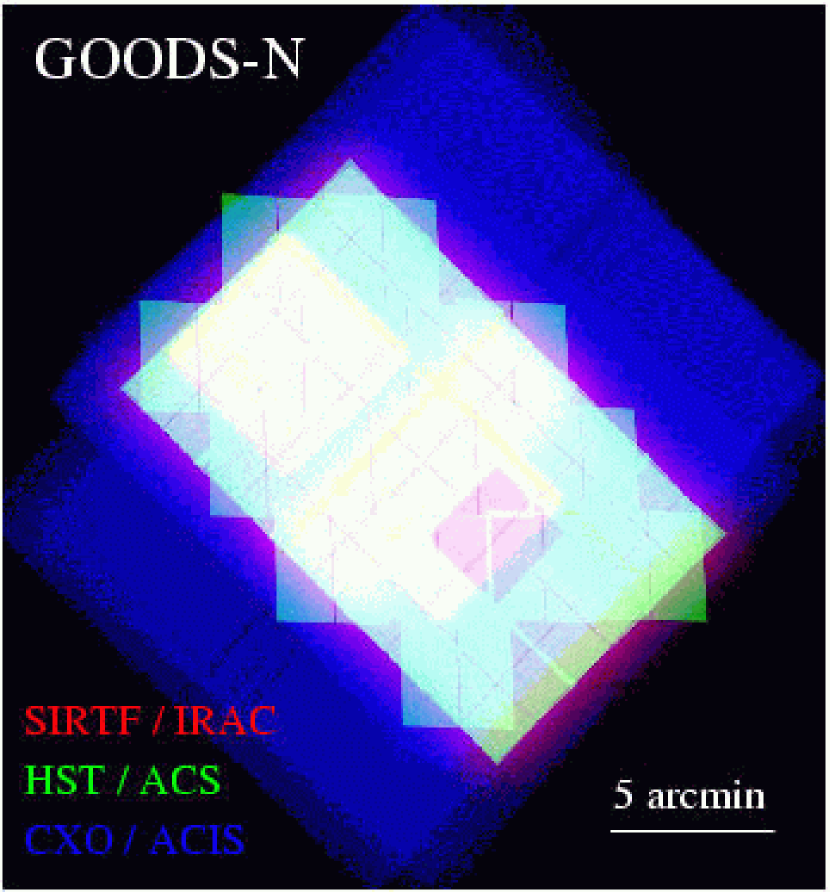
Figure 1: Exposure map of the GOODS HDF-N Observations. In this image, blue represents the Chandra (CXO) exposure map for the 2 Msec observations described by Alexander et al. (2003). Green represents the current HST/ACS exposure map, and red represents the planned SIRTF/IRAC exposure map. Where all fields overlap, the colors sum to give white in the representation. The different ACS tiling patterns on even and odd epochs produce the sawtooth pattern around the edge of the ACS fields. A guide-star failure on one of the ACS tiles produces the reddish square seen within the ACS rectangle. This exposure will be repeated to even out the final exposure map. The two planned 75-hour IRAC ultradeep fields can be seen faintly within the ACS area. These ultradeep fields are planned only for the HDF-N.

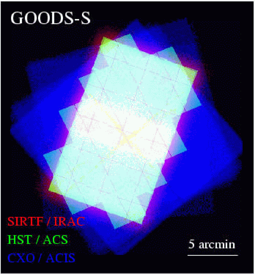
Figure 2: Exposure map of the GOODS CDF-S Observations. The color-map is the same as for Fig. 1. The Chandra observations are those of Giacconi et al. (2002).

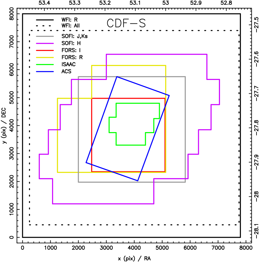
Figure 3: Schematic outline of the GOODS data sets in the CDF-S region. The blue shows the outline of the ACS area. The other colors outline the areas covered by the ESO data described in the text.

The data set discussed here includes ACS images, deep optical and near–infrared imaging from KPNO and ESO, and the CXO images. The main features of each data set are summarized in Table 1, while Table 2 lists the sensitivity achieved in each wavelength band. Figures 1 and 2 show the exposure maps of the three space–based data sets overlaid on top of each other to illustrate the extent of the area in common. Figure 3 shows a schematic of the layout of the existing imaging coverage in the CDF–S.

3 The HST ACS Data

The GOODS/ACS observations consist of imaging in the F435W, F606W, F775W and F850LP passbands, hereafter referred to as $B_{435}$, $V_{606}$, $i_{775}$ and $z_{850}$. While the $B_{435}$–band images were all acquired at the beginning of the survey, the $V_{606}$, $i_{775}$, and $z_{850}$–band images have been carried out in five epochs, separated by 40 to 50 days to optimize the search for high-redshift supernovae. Only 60% of the total exposure time in each field (3 epochs out of 5) in the $V_{606}$, $i_{775}$, and $z_{850}$are presented here, since the remainder of the data were not available at the time these papers were being prepared. In the odd–numbered epochs each $10\arcmin\times 16\arcmin$ field is tiled by a grid of $3\times 5$ individual ACS pointings, including some area of tile overlapping to check photometric and astrometric consistency. In even-numbered epochs, due to HST pointing constraints, the field is rotated by $45^{\circ}$ and a different overlapping tiling pattern is used, consisting of 16 separate pointings (see Figures 1 and 2). The complete set of $B_{435}$ observations were obtained in the first epoch alone, using the $3\times 5$ grid, with six exposures per position.

The exposure times at each epoch are typically 1050, 1050 and 2100 seconds in the $V_{606}$, $i_{775}$ and $z_{850}$ bands, respectively. These are subdivided into 2 exposures in each of the $V_{606}$ and $i_{775}$ bands, and into 4 exposures in the $z_{850}$ band. This strategy ensures good rejection of cosmic ray events in the single–epoch $z_{850}$ bands, which is where the detection of transients is carried out. Some cosmic rays remain in the $V_{606}$ and $i_{775}$ single–epoch images, which can nevertheless generally provide colors of the transients. In each case, the telescope field of view is shifted (“dithered”) by a small amount between individual exposures to allow optimal sampling of the point–spread function and to remove detector gaps and artifacts. The multiple epochs are later combined into a single mosaic, allowing cosmic ray rejection from at least six images per band. Except for the $B_{435}$ band, the mosaics used for the current papers were constructed from only three epochs of observations, and the total exposure times are approximately 7200, 3040, 3040, and 6280 seconds in the $B_{435}$, $V_{606}$, $i_{775}$, and $z_{850}$ bands, respectively.

Basic reduction of the raw data is carried out through calacs, the ACS calibration pipeline, which applies the basic calibration steps of bias subtraction, gain correction, and flat-fielding (Pavlovsky et al. 2002). The data received from the HST pipeline are then further processed by the GOODS pipeline using the multidrizzle script (Koekemoer et al. 2003), to create a set of geometrically rectified, cosmic-ray cleaned images (within a given epoch). These processed “tiles” are released as the “best-effort” GOODS public release v0.5 via the Multimission Archive at Space Telescope (MAST).

The early version of the geometric distortion model used in the basic processing described above proved to have significant problems matching sources in overlapping tiles. To rectify this, we derived an astrometric solution for each tile and each epoch based on sources matched in GOODS groundbased images. The reference for the CDF-S image was the $R$–band image of the field obtained as part of the ESO Imaging Survey (EIS) with the Wide Field Imager (WFI), which in turn was astrometrically calibrated to the Guide Star Catalog 2 (GSC-2) and put on the ICRS reference frame. For HDF–N, the reference image was an $R$-band Subaru image of the field (Capak et al. 2003).

The astrometric solution for the $z$-band mosaics has been derived by a least-squares optimization of the position, orientation, x and y pixel scales, and axis skew of each tile and epoch, minimizing the inter-epoch variations of the estimated position for $\sim 2000$ sources. The estimated rms in the source position, internal to the solution, is about 0.1 to 0.2 WFC pixels. For the other ACS bands, the astrometric solution is based on a tile-by-tile match to $z$-band source positions. These solutions had a residual rms of about 0.3 pixels, with larger deviations in some local regions across the field. All the exposures were then drizzled (Fruchter & Hook 2002) onto a series of images with a common pixel grid, in order to create a clean median image, which was subsequently used to create a cosmic ray mask for each exposure. Finally, the individual exposures were drizzled, using the new masks, onto a final single mosaic for each band, measuring 18000 by 24000 pixels with a scale of 0$\farcs$05/pixel.

For the purposes of the current papers the astrometric solution appears to be acceptable, although its deficiencies become apparent for bright stars, where the cosmic ray rejection algorithm rejects some good pixels due to the slight misregistrations. This can bias fluxes (faintward) for the brighter point sources in the $V_{606}$ and $i_{775}$ images (only). We have verified that there is little or no photometric effect for even slightly extended sources. A photometric comparison of the $V_{606}$ magnitudes (SExtractor MAG_AUTO values) in the original WFPC-2 HDF-N and the current mosaic reveals systematic biases of less than 0.01 magnitudes for galaxies in the range $23<$$V_{606}$$<26$, with an rms scatter less than 0.2 mag.

The resulting mosaics have a few remaining blemishes and some misregistrations between bands at the level of a fraction of a pixel. Slight sky level variations are also apparent. The masking of satellite trails, and reflection ghosts is not yet perfect, with residuals apparent in few places. The samples of galaxies used for the papers in this volume have all been individually inspected to remove objects that are thought to be artifacts. For most samples such contamination is negligible, but the contamination is significant for the single-band detections used to search for galaxies at $z\sim 6$, as discussed in detail by Dickinson et al. (2003).

4 The CXO Data

Chandra data in the GOODS fields were taken before the GOODS project began and are available from the CXO archive (Giacconi et al. 2002; Alexander et al. 2003). The integration times of the Chandra CDF–S and HDF–N observations total roughly 1 and 2 Msec, respectively. The GOODS SIRTF field layout was designed in part to maximize the coverage of the X–ray area. Subsequently, the ACS fields were designed to optimally cover both the SIRTF and Chandra fields. The CXO data for both fields have been re–analyzed in a self–consistent way, and new catalogs have been published by Alexander et al. (2003). Finally, these X–ray catalogs have been matched to the ACS catalogs by Koekemoer et al. (in preparation) for CDF–S and by Bauer et al. (in preparation) for HDF–N. Over 90% of the area covered by the GOODS ACS observations, the $S/N\geq 10$ point source sensitivity limits in the 0.5–2.0 keV and 2-8 keV bands, respectively, are $3.3$ and $24\times 10^{-16}$ erg s^-1 cm^-2 for the HDF–N and $4.3$ and $30\times 10^{-16}$ erg s^-1 cm^-2 for the CDF–S. The sensitivities at the CXO aim point, where the exposure time and image quality are maximized, are as much as a factor of $\sim 2$ and $\sim 4$ fainter for the CDF-S and HDF-N, respectively.

5 Ground–based Near–UV, Optical, and Near–IR Imaging

Ground–based imaging spanning a wide wavelength baseline is an important component of GOODS, and here, we describe the data that have been used for projects presented in this Special Issue. The CDF–S imaging consists of a complex arrangement of data sets covering different areas, often using multiple instrument pointings, as illustrated in Figure 3. These data sets were all placed on a common astrometric grid tied to the GSC2. The PSFs were matched by Gaussian convolution to a common FWHM of 0$\farcs$9. The WFI $U^{\prime}UBV$ images and a few of the images obtained with the New Technology Telescope (NTT) and the Superb–Seeing Imager (SOFI) have slightly poorer seeing, 0$\farcs$9–1$\farcs$05, but most projects use colors measured through $3\arcsec$ apertures, so this small mismatch should have little effect. The PSF–matched images were mosaiced onto a common $0\farcs 3$ pixel grid with the SWarp software (Bertin 2002). Noise maps were constructed for use in object detection and cataloging, carefully accounting for the effects of interpixel correlations. High–resolution ($0\farcs 15$/pixel) ISAAC mosaics were also made without degrading their excellent image quality. We have used the colors of stars to check the photometric zeropoints of the CDF–S data, as described below. Where possible, these were identified using the ACS imaging, using criteria for star–galaxy separation based on a diagram of peak surface brightness vs. isophotal magnitude. The same method was used on the ground–based data to extend the stellar sample to areas beyond the ACS coverage.

5.1 KPNO 4m + MOSAIC $U$–band imaging

Deep $U$–band images of the GOODS HDF–N field were obtained using the prime focus MOSAIC camera on the KPNO Mayall 4–m telescope in March 2002. A total of 27.5 hours of exposure time were obtained in photometric conditions with mean seeing FWHM $=1\farcs 15$. We reduced the data using the IRAF mscred package, which carries out bias subtraction, flat–fielding, correction for geometric distortion, removal of amplifier cross–talk, subtraction of an additive “pupil ghost”, image registration, and combination.

5.2 ESO–MPI 2.2–m + WFI imaging

An area of $\sim 0.4$ sq. degree around the CDF-S was surveyed with WFI on the ESO–MPI 2.2–m telescope using the $U^{\prime}UBVRI$ passbands. Much of these data were obtained as part of the EIS, and are described in Arnouts et al. 2001. Additional $BVR$ images were obtained for the GOODS program and in the course of the COMBO–17 project (Wolf et al. 2001). The EIS, GOODS, and COMBO data were reduced in a uniform fashion using the GaBoDs WFI reduction pipeline (Schirmer et al. 2003). We carefully checked the accuracy of the photometric calibration using the color loci of stars. These were compared to synthetic color-color diagrams generated using the Gunn & Stryker (1983) spectrophotometric library, convolved with the instrumental passbands. Zeropoints were adjusted as necessary, and are accurate to $<0.1$ mag.

5.3 ESO VLT + FORS1 imaging

Additional, deep $R$ and $I$-band images were obtained with the ANTU telescope (UT1) at the VLT, using the FORS1 instrument. The data and their reduction are described in Tozzi et al. (2001). The FORS1 images cover only a portion of the GOODS CDF–S field using several pointings with variable exposure time. A portion of the field is covered by relatively short $R$–band exposures. The core region ($13\farcm 6\times 13\farcm 6$) is quite deep, however, and in particular is much deeper than the WFI imaging in the $I$–band. The photometric zeropoints were checked and adjusted by comparing photometry for stars and galaxies in the WFI and FORS1 images, accounting for the passband differences, and agree on average to $<0.05$ mag.

5.4 ESO NTT + SOFI imaging

Near–infrared data in the $J$ and $K_{s}$ bands for the CDF–S were obtained with SOFI on the NTT as part of the EIS. The observations and reductions are described in Vandame et al. 2001. They consist of a 4$\times$4 grid of pointings covering 0.1 sq. deg. SOFI $H$-band data were obtained and reduced by Moy et al. 2002, and cover a larger area. Photometric zero-points were checked by comparing photometry of stars to measurements from the Two-Micron All-Sky Survey (2MASS).

5.5 ESO VLT + ISAAC imaging

The GOODS program is gathering a mosaic of very deep $JHK_{s}$ images with ISAAC on the VLT as part of an ESO Large Programme. Ultimately, 32 pointings will be used to cover the GOODS CDF–S field. Data for 8 fields were obtained in 2001–2 and combined with ISAAC data from an ESO visitor program, kindly provided by E. Giallongo. These images cover only $\sim 50$ arcmin², but are much deeper than the SOFI data, with excellent image quality (mean FWHM $\approx 0\farcs 45$). They were reduced with the EIS pipeline. Their photometric zeropoints were adjusted to a common scale by comparison to objects in the SOFI images, and agree within 0.07 mag.

6 Source Catalogs

Several different source catalogs for the ACS and ground–based images are used in the accompanying papers. In all cases, source identification and photometry were performed using SExtractor (Bertin & Arnouts 1996). Simulations were used to guide the choice of detection thresholds and the size and shape of the convolution kernel to optimize the detection of faint galaxies while keeping spurious sources to a minimum. Photometric uncertainties within any aperture are computed using the normalized noise maps that were produced as part of the data reduction process. However, some projects use detailed simulations with artificial sources to assess the true photometric errors.

For the ACS catalog, sources were detected in the $z_{850}$ mosaic, and photometry was carried out through matched apertures in the other ACS bands. Several different ground–based catalogs were generated for the CDF–S, with detections based on the WFI $R$–band, SOFI $K$–band, and ISAAC $K$ and $J$–bands. In each case, matched aperture photometry was measured for all of the other CDF–S ground–based images. A wide–field HDF–N catalog, based on Subaru $BVRIz$ imaging and the GOODS KPNO $U$ data, is presented by Capak et al. 2003, but is not used in the present set of Letters. Where needed, ACS–to–ground–based colors were measured using images degraded to match the ground–based PSFs. These provide optical–IR colors of ACS sources, as well as $U-B_{435}$ colors for Lyman break color selection.

Photometric redshifts for galaxies in the CDF–S (Mobasher et al. 2003) were estimated using all of the available photometry ($U$ through $K_{s}$ bands) and the BPZ software of Benítez (2000). They were tested against spectroscopic redshifts from the K20 survey (Cimatti et al. 2002), kindly provided by A. Cimatti, and also against redshifts measured with VLT+FORS2 for the GOODS program.

7 Sensitivity

The sensitivity of the images depends on the sizes and shapes of the objects of interest. To guide the readers of these Letters, Table 2 provides two sensitivity estimates (point source flux and limiting surface brightness) for each of the GOODS space– and ground–based imaging data sets. These should be taken as representative values only, since the actual depths of the imaging data sets vary over the field of view, and depend on the details of source size, PSF shape, crowding, etc.

Many of the papers in this issue rely on SExtractor detections in the ACS $z_{850}$-band image. To assess the completeness limits for this catalog, we have iteratively inserted sources into the image and re-run SExtractor. This is the standard procedure used for point-source photometry to assess completeness and photometric errors in color-magnitude diagrams. The problem has more dimensions for galaxy photometry because the detectability of a galaxy depends on the size and surface brightness profile. Our simulations uniformly populate the magnitude range $20<z_{850}<28$ and the range of galaxy half-light radii $0\farcs 01<r<1\farcs 5$. The input galaxies are a 50/50 mix of spheroids — galaxies with $r^{1/4}$-law surface-brightness profiles — and disks with exponential surface-brightness profiles. The spheroids are assumed to be oblate and optically thin with an intrinsic axial ratio distribution that is uniform in the range $0.3<b/a<0.9$. The disks are modeled as optically-thin oblate spheroids with a (very flat) intrinsic axial ratio of $b/a=0.05$. Galaxies are viewed from random inclinations. The simulated galaxies are convolved with the PSF and inserted into the $z$-band image without additional Poisson noise. For bright sources, the noise is thus slightly underestimated, but for faint sources, the sky background completely dominates anyway so this shortcut does not affect the results. The resulting completeness limits in a plane of magnitude and half-light radius are shown in Fig. 4.

8 Summary

The intent of this paper has been to provide a brief overview of the GOODS project and to describe the data used to derive the scientific results discussed elsewhere in this issue. The GOODS web site, which can be accessed from http://www.stsci.edu/ftp/science/goods/, provides further details of the project and access to the GOODS data.

Table 1: The Data

Facility	Passbands	Area coverage	Angular resolution	Field
HST + ACS	$BViz$	320	0.125	HDF-N + CDF-S
CXO+ ACIS	0.5-8 keV	450	0.85–10	HDF-N
CXO+ ACIS	0.5-8 keV	390	0.85-10	CDF-S
KPNO 4-m + MOSAIC	$U$	1800	1.15	HDF-N
ESO 2.2-m + WFI	$U^{\prime}UBVRI$	$>$1350	0.85–1.05	CDF-S
ESO VLT + FORS1	$RI$	175	0.6–0.8	CDF-S
ESO NTT + SOFI	$JK_{s}$	360	0.65-1.05	CDF-S
ESO NTT + SOFI	$H$	630	0.55-0.85	CDF-S
ESO VLT + ISAAC	$JHK_{s}$	50	0.40-0.65	CDF-S

Table 2: Sensitivity for Current GOODS Optical and Near–Infrared Data

Facility	$U^{\prime}$	$U$	$B$	$V$	$R$	$I$	$z$	$J$	$H$	$K_{s}$
HST+ACS	$\cdots$	$\cdots$	27.8	27.8	$\cdots$	27.1	26.6	$\cdots$	$\cdots$	$\cdots$
HST+ACS	$\cdots$	$\cdots$	28.4	28.4	$\cdots$	27.7	27.3	$\cdots$	$\cdots$	$\cdots$
4–m MOSAIC	$\cdots$	25.9	$\cdots$	$\cdots$	$\cdots$	$\cdots$	$\cdots$	$\cdots$	$\cdots$	$\cdots$
4–m MOSAIC	$\cdots$	29.0	$\cdots$	$\cdots$	$\cdots$	$\cdots$	$\cdots$	$\cdots$	$\cdots$	$\cdots$
2.2–m WFI	25.0	24.7	26.2	25.8	25.8	23.5	$\cdots$	$\cdots$	$\cdots$	$\cdots$
2.2–m WFI	28.1	27.9	29.3	28.9	28.9	26.6	$\cdots$	$\cdots$	$\cdots$	$\cdots$
VLT FORS1	$\cdots$	$\cdots$	$\cdots$	$\cdots$	26.2	25.9	$\cdots$	$\cdots$	$\cdots$	$\cdots$
VLT FORS1	$\cdots$	$\cdots$	$\cdots$	$\cdots$	29.4	29.0	$\cdots$	$\cdots$	$\cdots$	$\cdots$
NTT SOFI	$\cdots$	$\cdots$	$\cdots$	$\cdots$	$\cdots$	$\cdots$	$\cdots$	22.8	22.0	21.8
NTT SOFI	$\cdots$	$\cdots$	$\cdots$	$\cdots$	$\cdots$	$\cdots$	$\cdots$	25.9	25.1	25.0
VLT ISAAC	$\cdots$	$\cdots$	$\cdots$	$\cdots$	$\cdots$	$\cdots$	$\cdots$	25.5	24.9	25.1
VLT ISAAC	$\cdots$	$\cdots$	$\cdots$	$\cdots$	$\cdots$	$\cdots$	$\cdots$	27.9	27.3	27.4

Figure 4: Completeness limits for the GOODS ACS $z$-band catalog as a function of galaxy total magnitude and half-light radius. The contours show the percentage of galaxies recovered by SExtractor in the simulations described in the text.

References

- (1)
- (2) Alexander, D., et al., 2003, AJ, in press, astro-ph/0304392
- (3) Arnouts, S., et al., 2001, A&A, 379, 740
- (4) Benítez, N., 2000, ApJ, 536, 571
- (5) Bertin, E., 2002, SWarp User’s Guide
- (6) Bertin, E., and Arnouts, S., 1996, A&A, 117, 393
- (7) Bunker, A., Smith, J., Spinrad, H., Stern, D. & Warren, S., 2003, astro-ph/0303290.
- (8) Capak, P., et al., 2003, ApJ, submitted
- (9) Cimatti, A., et al., 2002, A&A, 392, 395
- (10) Cohen, J., Hogg, D. W., Blandford, R., Cowie, L. L., Hu, E. Songaila, A., Shopbell, P. & Richberg, K., 2000, ApJ, 538, 29
- (11) Dawson, S., McCrady, N., Stern, D., Eckart, M., Spinrad, H., Liu, M., & Graham, J. R., 2002, astro-ph/0212240
- (12) Dickinson, M., et al., 2003, this volume.
- (13) Ferguson, H. C., Dickinson, M., & Williams, 2000, ARAA, 38, 667
- (14) Fruchter, A. S. & Hook, R. N. 2002, PASP 114, 144
- (15) Giacconi, R. et al., 2002, ApJS, 139, 369
- (16) Gunn, J., & Stryker, 1983, ApJS, 52, 121
- (17) Koekemoer, A. M., Fruchter, A. S. Hack, W. & Hook, R. N. 2003, HST Calibration Workshop (STScI: Baltimore)
- (18) Madau, P., Pozzetti, L., & Dickinson, M. E. 1998, ApJ, 498, 106
- (19) Mobasher, B., et al., this volume
- (20) Moy E., et al. 2002, astro-ph/0211247
- (21) Oke, J. B. 1974, ApJS, 27, 21
- (22) Pavlovsky, C., et al. 2002, ACS Instrument Handbook, Version 3.0, (Baltimore: STScI).
- (23) Riess, A., et al., 2003, this volume
- (24) Roche, N., Dunlop, J. & Almaini, O., 2003, astro-ph/0303206
- (25) Schirmer, M., Erben, T., Schneider, P., Pietrzynski, G., Gieren, W., Micol, A., Pierfederici, F. 2003, astro-ph/0305172
- (26) Somerville, R. S., et al., 2003, this volume
- (27) Spergel, D., et al., 2003, ApJ, submitted
- (28) Stanway, E., Bunker, A., & McMahon, R., 2003, astro-ph/0302212
- (29) Steidel, C. C., Giavalisco, M., Pettini, M., Dickinson, M., & Adelberger, K. 1996, ApJ,
- (30) Tozzi, P., et al., 2001, ApJ, 562, 42
- (31) Vandame, B., et al., 2001, A&A, submitted (astro-ph/0102300),
- (32) Williams, R. E. et al. 1996, AJ, 112, 1335
- (33) Williams, R. E. et al. 2000, AJ, 120, 2735
- (34) Wolf, C., Dye, S., Kleinheinrich, M., Meisenheimer, K., Rix, H.-W., & Wisotzki, L., 2001, A&A, 377, 442
- (35) Yan, H., Windhorst, R. A., Röttgering, H. J., Cohen, S. H., Odewhan, S. C., Chapman, S. C. & Keel, W. C., 2003, ApJ, 585, 67
- (36)