The Mass Ratio Distribution in Main-Sequence Spectroscopic Binaries Measured by IR Spectroscopy

Abstract

We report infrared spectroscopic observations of a large, well-defined sample of main-sequence, single-lined spectroscopic binaries in order to detect the secondaries and derive the mass ratio distribution of short-period binaries. The sample consists of 51 Galactic disk spectroscopic binaries found in the Carney & Latham high-proper-motion survey, with primary masses in the range of 0.6–0.85 M_⊙. Our infrared observations detect the secondaries in 32 systems, two of which have mass ratios, $q=M_{2}/M_{1}$, as low as $\sim 0.20$. Together with 11 systems previously identified as double-lined binaries by visible light spectroscopy, we have a complete sample of 62 binaries, out of which 43 are double-lined. The mass ratio distribution is approximately constant over the range $q=1.0$ to 0.3. The distribution appears to rise at lower $q$ values, but the uncertainties are sufficiently large that we cannot rule out a distribution that remains constant. The mass distribution derived for the secondaries in our sample, and that of the extra-solar planets, apparently represent two distinct populations.

1 Introduction

The mass ratio distribution of binaries provides one of the few diagnostics for testing models of binary formation (for recent reviews, see Clarke 2001; Tohline 2002; Halbwachs et al. 2003). However, the use of the mass ratio distribution in spectroscopic binaries (SBs) has been limited because, in most studies, only the primary spectrum is detected. Without the secondary radial velocities, the mass ratio of a spectroscopic binary cannot be measured. Detection of the secondary spectrum is difficult because most radial velocity observations are made in visible light, where the luminosity of stars less massive than $\sim 1$ M_⊙ is a strong function of the mass (e.g., Carney et al. 1994, hereafter CL94). As a result, the measured secondary/primary mass ratios, $q=M_{2}/M_{1}$, are clustered close to 1. To overcome this bias astronomers have applied powerful statistical techniques to samples of single and double-lined spectroscopic binaries (SB1s and SB2s), in order to derive the mass ratio distribution down to mass ratios as low as $\sim 0.1$ (e.g., Halbwachs 1987; Heacox 1995). However, because of the missing information on the mass ratios of the binaries, the resolution ability of the statistical techniques is limited, and they can only derive the gross features of the distribution. This might be the reason why the results of such analyses still differ and a consensus on the underlying distribution has not been reached.

Goldberg, Mazeh & Latham (2003, hereafter G03) studied 129 binaries identified in the Carney & Latham high-proper-motion sample (CL94), which consisted of a large fraction of halo stars. Their sample of binaries included 25 SB2s. G03 found a rise in the distribution as the mass ratio decreases to $q\sim 0.2$, a drop at $q<0.2$, and a small peak at $q\sim 0.8$. Halbwachs et al. (2003) considered a well-defined sample of 27 binaries within the nearby F7 to K stars, together with 25 binaries found in the open clusters of Pleiades and Praesepe. Their sample of 52 binaries consisted of 15 SB2s, for which the mass ratios were directly derived, another 9 binaries with mass ratios estimated from astrometric data (Udry et al. 2003), and an additional 7 cluster binaries with mass ratios estimated from their photometric properties. Halbwachs et al. found a mass ratio distribution with two peaks: a broad, shallow, peak between $q\sim 0.2$ and $\sim 0.7$, and a sharp, high, peak at $q>0.8$. The latter appears only in the distribution of the short period binaries, with periods shorter than 50 days.

Evidently, even the most recent studies do not agree on the true mass ratio distribution. It is therefore desirable to derive the mass ratio distribution with minimal need for statistical tools. To accomplish this we need a large, well defined sample of binaries dominated by SB2s with mass ratios measured over as large a range as possible. Our approach to the detection of main-sequence and pre$-$main-sequence (PMS) SB2s is to observe with high resolution, infrared (IR) spectroscopy SB1s that were previously identified and measured with visible light (Mazeh et al. 2002; Prato et al. 2002a,b). Because the secondaries in SB1s are cool, the secondary to primary light ratio is greater in the IR than in visible band, favoring their detection in the IR. One result of this approach is the smallest mass ratio ever measured dynamically in a PMS SB, $q=0.18\pm 0.01$, in the NTTS 160905$-$1859 system (Prato et al. 2002a).

To compile as complete and large as possible a sample for study, we chose to use a subsample of the SBs in the Carney & Latham study of 1464 high-proper-motion, nearby, late G and early K, main-sequence stars (CL94). Systematic, long term radial velocity monitoring of these stars in visible light has identified 171 SB1s and 34 SB2s (Latham et al. 2002, hereafter L02; Goldberg et al. 2002, hereafter G02). Out of these, we focused on 51 SB1s, turning 32 systems into SB2s. The composition of our sample is described in §2, the observations in §3, the analysis in §4, and the measured and derived mass ratio distribution in §5. We compare our results with previous studies in §6, discuss our results in §7 and conclude the discussion in §8.

2 The Sample

We selected SB1s from L02 with a well defined range of metallicities and distances, as derived by CL94 using photometry, color indices in the visible and IR, and low S/N spectroscopy. To exclude the halo stars from our sample and to include stars with relatively strong spectral lines we chose only stars identified by G03 as Galactic disk stars, with metallicities $[Fe/H]\stackrel{{\scriptstyle>}}{{\sim}}-1$. To ensure high S/N ratio in the observations, and to choose a volume limited sample, we excluded all stars whose distances were estimated by CL94 to be larger than 90 pc. The SB sample identified by L02 and G02 was not complete for binaries with long periods (see discussion in G03), so we chose only binaries with periods shorter than 3000 days.

Table 1 lists the 52 SB1s observed. The system $V$-band magnitude, metallicity, estimated distance, and binary period, taken from L02 and CL94, appear in columns (4)–(7). Our sample is characterized by $V<11.46$ mag (which corresponds to $H\stackrel{{\scriptstyle<}}{{\sim}}9.6$ mag for these stars) and $[Fe/H]>-1.09$. Column (8) of Table 1 lists the mass estimates of the primaries, as derived by CL94.

Analysis of a single-lined orbit yields the mass function,

$$f(M)={(M_{2}~{}sin~{}i)^{3}\over(M_{1}+M_{2})^{2}}={q^{3}\over(1+q)^{2}}M_{1}sin^{3}i$$

where $i$ is the orbital inclination. Using the estimate of the primary mass and the limit of an edge on orbit, $i=\pi/2$, $f(M)$ determines the minimum mass ratio $q_{min}$. We used the mass functions reported by L02 to calculate the values of $q_{min}$ for the SB1s in our sample and listed these in column (8) of Table 1. The uncertainties include that of the mass function and our estimate of $\pm 0.1$ M_⊙ for the uncertainty of $M_{1,est}$. During the analysis we found that one system in Table 1, G17-22, has a minimum mass ratio substantially larger than unity, $1.36\pm 0.13$. This probably indicates a white dwarf secondary that was originally the primary star. If this is true, the mass ratio of the system now differs from its original value. We therefore excluded this system from further analysis.

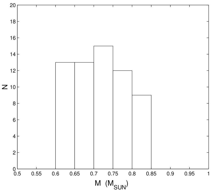
Figure 1: The distribution of primary masses, $M_{1,est}$, as estimated by CL94, in the entire sample of 62 binaries analyzed in this study — 11 SB2s identified in visible light by GO2, and 51 SB1s observed by high resolution IR spectroscopy.

For completeness we included in our analysis the SB2s already detected by G02 which have the same limits on distance, metallicity, and period as the SB1s in Table 1. Table 2 lists these 11 binaries and is organized in the same way as Table 1, except that the last column lists the mass ratio measured by G02. Our study of the mass ratio distribution of nearby main-sequence SBs is thus based on 62 systems, the 11 SB2s in Table 2 with measured $q$’s, all close to 1, and the 51 SB1s in Table 1 (excluding G17-22). Figure 1 shows the distribution of $M_{1,est}$ in the entire sample of 62 SBs. The range of the masses is quite narrow, 0.6–0.85 M_⊙, with a median value of $0.72$ M_⊙.

Our sample definition relies on CL94’s distances rather than HIPPARCOS measurements, because only the former are available for all the systems in our sample, and the latter have large uncertainties at distances greater than $\sim 60$pc. Photometric distances might be biased towards smaller distances for binaries with high mass ratios, as the secondaries make such binaries brighter than single stars. Such bias could have introduced the Öpik effect (Öpik 1926; Branch 1976) into our sample of binaries. To look for such an effect we considered the ratio of the Hipparcos distance over the CL distance for each of the binaries in our sample. If the Öpik was present in our sample we would expect the ratio to be larger for binaries with mass ratio close to unity. To investigate this possibility, we divided our sample into two subsamples, with $q_{min}$ above and below $0.85$. The average and r.m.s of the ratios of the high and low mass ratio samples were $1.12\pm 0.26$ and $1.29\pm 0.39$, respectively. The difference between the two figures is insignificant, and certainly not in the direction expected for the Öpik effect. We conclude that there is no evidence that the Öpik effect has contaminated our sample.

3 Observations and Data Reduction

Observations of all stars in Table 1 were made with the NIRSPEC spectrometer at the Keck II telescope (McLean et al. 1998, 2000), following the procedures described by Prato et al. (2002a,b). The spectrometer was centered on 1.55 $\mu$m in order 49. Exposure times were long enough to obtain spectra with S/N $\gtrsim 100$ on each target, typically between 5 and 10 minutes. The observations in June, 2000, and January, 2001, were obtained using adaptive optics (AO) and achieved resolution R $\sim 30,000$. Observations in February, May, and June, 2001, were made without the AO system and have resolution R $\sim 24,000$. A few more spectra for some of the systems were obtained when time permitted in subsequent observing runs; these later observations were all in the non-AO mode. The modified Julian dates of observation for each binary in the sample are listed in Table 3, column (2). The spectra were extracted and wavelength calibrated using the REDSPEC software package. We used only order 49 for the results presented here because it is almost completely free of terrestrial absorption lines.

As in our previous studies (Mazeh et al. 2002; Prato et al. 2002a,b), we used the TODCOR two-dimensional correlation algorithm (Zucker & Mazeh 1994) and our library of stellar templates to analyze the target spectra for the velocities of the primary and secondary stars. Table 3 lists the derived velocities of the primary, $v_{1}$, and the secondary, $v_{2}$, and their uncertainties, as yielded by TODCOR. The uncertainties do not include the errors induced by the scatter of the radial velocities assigned to the templates, which we estimate to be of the order of 1 km s^-1. The latter were added when we used these velocities for the orbital solution.

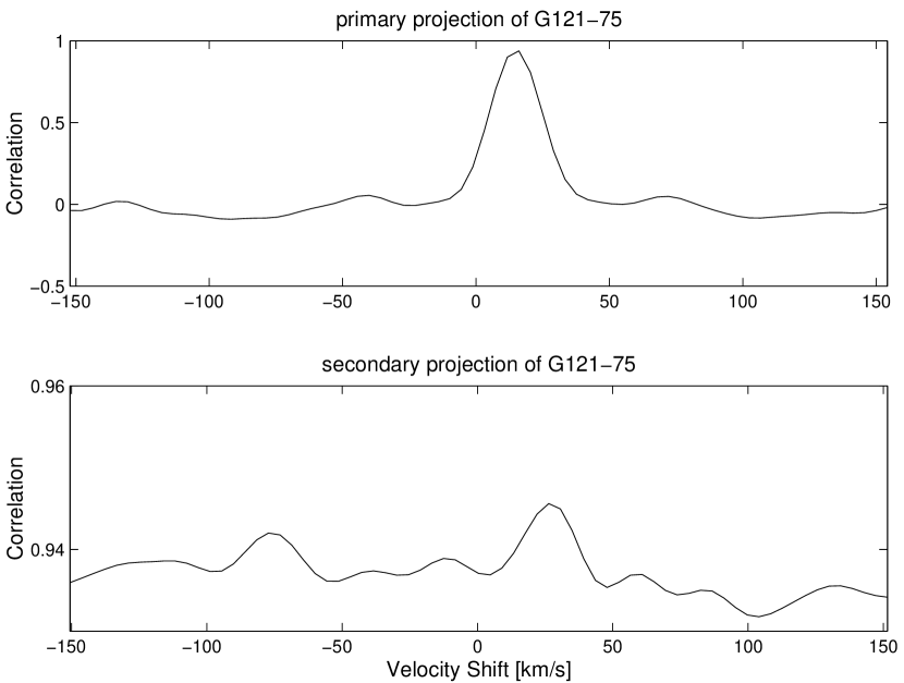
Figure 2: TODCOR output for the spectrum of SB2 G121-75, obtained on 2 May, 2001 (UT), exhibiting two aspects of the two-dimensional correlation function. The top panel shows the correlation as a function of the primary template shift, when the velocity of the secondary template is held fixed at the value that yielded maximum correlation. The lower panel shows the correlation as a function of the secondary template shift, when the velocity of the primary template is held fixed at the value that yielded maximum correlation. Note the different scales of the two panels.

The primary velocity was detectable in every observation of each target, whereas not all spectra yielded a reliable measurement of the secondary velocities. This is because the correlation peak of the secondary was not always sufficiently prominent because of several possible factors including the secondary to primary light ratio, the inevitable differences between the spectra of the SB components and their corresponding templates, small velocity differences between the components, and the S/N ratio of the observed spectra. The last two factors may vary between one observation and another, which explains why a reliable secondary velocity may be obtained from one spectrum of an object and not from another. For our analysis we chose only spectra that yielded correlation functions for which we judged the secondary peak to be well determined. An example of the derived correlation is given in Figure 2, which shows two aspects of the two-dimensional correlation function of one spectrum of G121-75, for which we estimate the flux ratio to be $0.08\pm 0.01$. The relatively small flux ratio caused the increase of the correlation function at the secondary velocity to be minute, from $\sim 0.935$ to $\sim 0.945$, as can be seen from the lower panel of the figure. Nevertheless, the peak is well above the noise.

Our criteria led us to accept only 58 secondary velocities out of 112 observations. The primary and secondary velocities, and their $1\sigma$ uncertainties are listed in Table 3, columns (3)–(6). Out of the 51 systems in the IR sample, we have derived the secondary radial velocities for 32 systems. For convenience, columns (2) and (3) of Table 4 list the numbers of times that a target was observed and the secondary detected.

4 Double-Lined Orbital Analysis

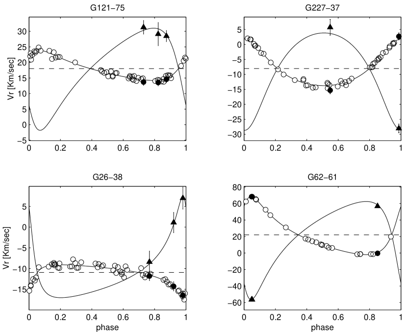
Figure 3: Double-lined orbital solution for four SB2s. The open circles present previously measured velocities of the primary (L02). The filled circles and triangles mark the primary and secondary velocities measured by this work. The solid lines present the calculated orbital solutions.

In all the 32 binaries for which we measured the secondary velocity, we derived new SB2 orbital solutions using our measured values of $v_{1}$ and $v_{2}$ together with the primary velocities of L02. All the newly derived elements were consistent with the SB1 elements of L02. The mass ratios of each binary, $q_{orb}$, were derived from the ratio of the primary and secondary semi-amplitudes, $K_{1}$ and $K_{2}$, and are listed in column (4) of Table 4. $K_{1}$ was determined by combining the many radial velocities of L02 with our few additional measurements, and is therefore well established. On the other hand, $K_{2}$ was determined only by our few secondary velocity measurements, and is therefore less robust. We have more than one radial velocity measurement of the secondary for only 14 systems. Examples of the orbital solutions for 4 binaries are plotted in Figure 3. All $v_{2}$ measurements in these 14 systems are within 1$\sigma$ of the best fit orbital solution.

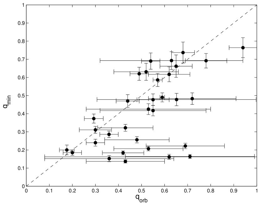
Figure 4: Minimum mass ratio as a function of the measured mass ratio for the 32 SB2s in which IR spectroscopy detected the secondary. The dashed line equation is $q_{min}=q_{orb}$.

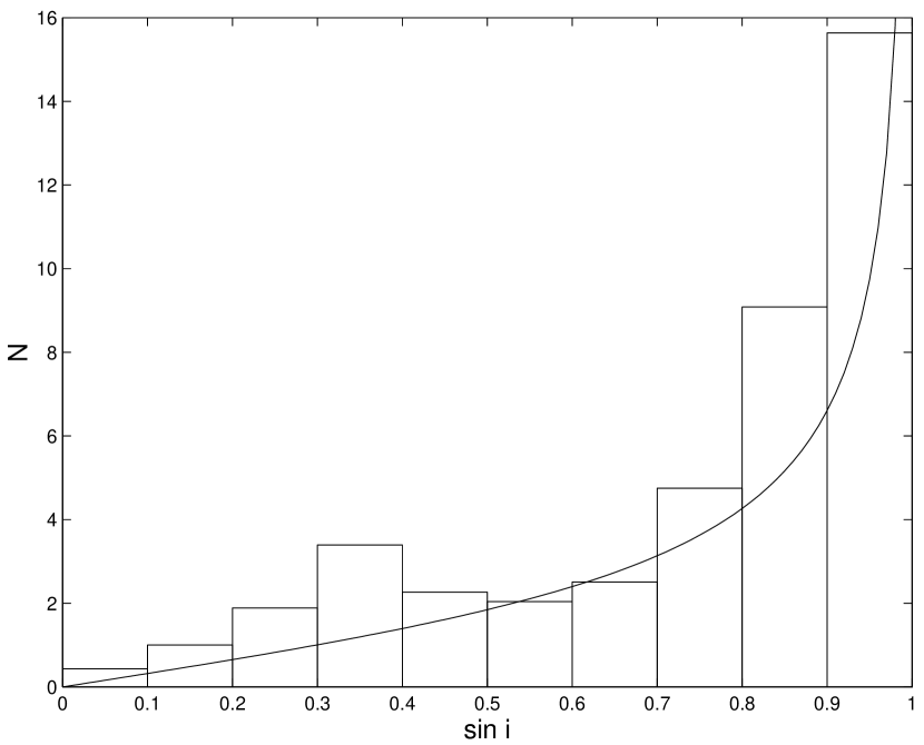
Figure 5: Histogram of derived $\sin~{}i$, as calculated from the mass function, $q_{orb}$, and $M_{1,est}$ for the 32 SB2s detected by IR spectroscopy and the 11 SB2s detected by G02. The solid line shows the expected distribution for randomly oriented orbits.

For 18 of the systems we have only one $v_{2}$ measurement, 4 of which have $q_{orb}$ values of low statistical significance, $q_{orb}/\sigma<2$. Two tests give us confidence that the set of $q_{orb}$’s we have derived are reliable. Clearly, we expect $q_{min}<q_{orb}$. Figure 4 plots $q_{min}$ as a function of $q_{orb}$, showing that the derived values of $q_{orb}$ are either greater than their corresponding value of $q_{min}$ or within 2$\sigma$ of the difference. Using the derived $q_{orb}$ values with the corresponding estimated masses, we can also derive $\sin i$. In Figure 5 we plot the distribution of the derived $\sin i$, together with the expected distribution for a sample of randomly oriented orbits in space. The two are very similar, again supporting our working assumption that the derived $q_{orb}$ are correct.

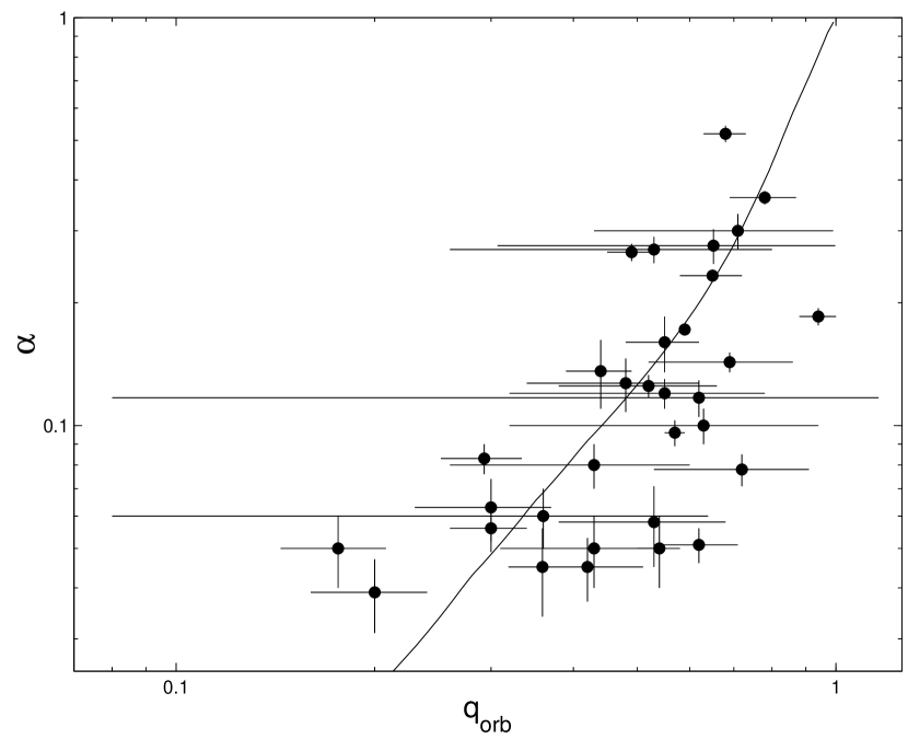
Figure 6: The secondary/primary flux ratio at $1.55\mu$m, $\alpha$, vs. $q_{orb}$ for the SB2s detected by IR spectroscopy. The solid line shows the theoretical $H$-band flux ratio vs.  mass ratio according to the calculations of Baraffe et al. (1998) for $M_{1}=0.7$ M_⊙, [Fe/H] = 0, and Age 5 Byr.

TODCOR analysis also provides the flux ratio, $\alpha$, at which the combination of shifted templates for the secondary and primary stars yields the maximum correlation. The last column of Table 4 lists our best estimate for $\alpha$ at $1.55\mu$m, averaged over several measurements when they were available. The derived ratios cannot be exact because of the unavoidable mismatch between the actual effective temperatures and metallicities of the primary and secondary stars and those of the templates used in the TODCOR analysis. Nevertheless, the derived values give a rough estimate of the true values. To show that this is the case, Figure 6 plots the estimated flux ratio as a function of the measured mass ratio. The solid line shows the light ratio in the photometric $H$-band for Baraffe et al.’s (1998) models of low-mass main-sequence stars at age 5 Byr with [Fe/H]=0, referenced to primary mass of 0.7 M_⊙. Our measured values are roughly consistent with the theoretical values. The large scatter is probably attributable to the approximate nature of the measured $\alpha$, the range of metallicities and ages of the targets, and to the fact that the model values integrate stellar spectra over the $\sim 0.28\mu$m width of the $H$-band filter while our spectra in NIRSPEC order 49 span only $\sim 0.022\mu$m.

Figure 6 shows that detection of secondaries by IR spectroscopy extends down to $\alpha\sim 0.04$. Below this light ratio, our spectra in NIRSPEC order 49 do not yield reliable secondary velocities through the analysis described here. As we discuss in the next section, this is associated directly with the minimum mass ratio to which our observations are sensitive.

5 The Mass Ratio Distribution

Our new measurements of the mass ratio extend down to $q=0.20\pm 0.04$ and $0.18\pm 0.03$ for G14-54 and G255-45, respectively (Table 4). To our knowledge, these are the lowest mass ratios yet measured dynamically in a detached main-sequence binary in which the primary is a G or K spectral type star. They are matched only by our work on PMS stars (Prato et al. 2002a). Together with the 11 SB2s in Table 2, dynamically derived mass ratios are now available for 43 of the 62 binaries in our sample.

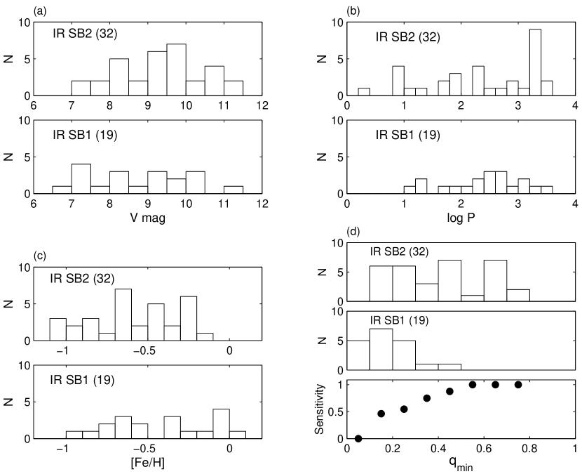
Figure 7: Comparison of the distributions of the $V$-band magnitude (upper left), period (upper right), metallicity (lower left), and minimum mass ratio (lower right) for the 32 SB2s in which the secondaries were detected by IR spectroscopy, and for the 19 binaries in which the secondaries remain undetected. In the distribution with respect to the minimum mass ratio, the bottom panel shows the sensitivity for detection given as (number detected/total number) for each bin of width $\Delta q_{min}=0.1$.

What is the nature of the binaries in which IR spectroscopy did not detect the secondary? There seem to be no significant differences in the distributions of brightness, period, or metallicity (Figure 7a,b,c) of the binaries with and without IR detections of the secondary. Applying a two-sample Kolmogorov-Smirnov (K–S) test to these three distribution pairs yields significance values of $0.47$, $0.45$ and $0.15$, respectively. Figure 7d suggests, however, that the systems with secondaries undetected in the IR have systematically lower $q_{min}$’s than those with detected secondaries. The K–S test shows that difference in the two distributions is very significant; the probability that they are drawn from the same distribution is only $5.6\times 10^{-4}$. This suggests that systems with low $q_{min}$, and hence small $M_{2}$, are undetected probably because their secondary/primary light ratio falls below our sensitivity limit.

The lowest panel of Figure 7d displays our detection limit more directly. For each bin of width $\Delta q_{min}=0.10$, the abscissa plots the ratio of the number of binaries with IR detected secondaries to the number of binaries having $q_{min}$ in that bin. The figure indicates that our observations detected all systems with $q_{min}>0.5$, and have monotonic decreasing sensitivity below that value. Taken together, the distribution of non-detections in the middle panel, and the sensitivity plotted in the lower panel, indicate that most of the undetected secondaries in binaries with $q_{min}$ below $0.5$ probably have actual mass ratios that are smaller than 0.5. If their $q$’s were larger, we probably would have detected them.

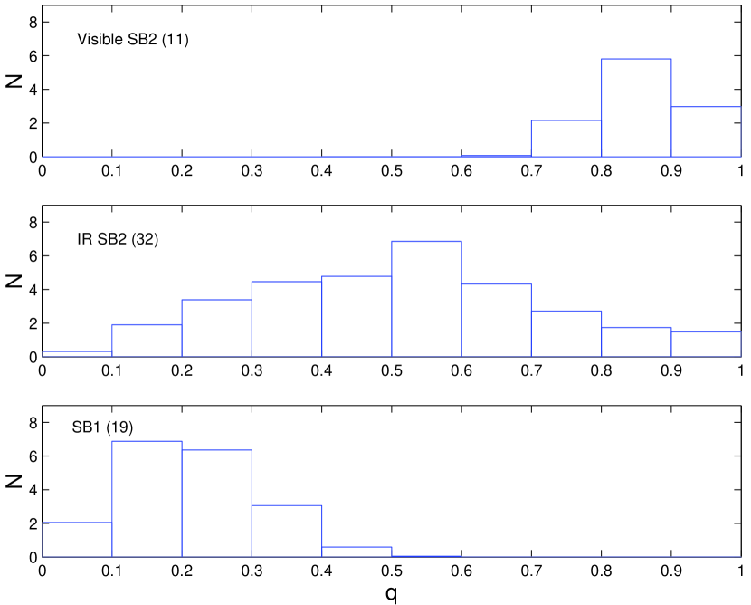
Figure 8: The distribution of mass ratios in our sample in bins of width $\Delta q=0.1$. Top panel — measured in visible light (G02), middle panel — measured in the IR (this work), and bottom panel — the distribution for the 19 SB1s remaining in our sample, estimated with Mazeh and Goldberg (1992) algorithm (see text, and compare with middle panel of Figure 7d).

The top and middle panels of Figure 8 show the distribution of mass ratios of the SB2s as detected in visible light by G02 and in the IR, as described here. To allow for the uncertainties of the mass ratios we distributed each binary as a Gaussian centered on its measured $q$ value, with a width equal to its estimated uncertainty. The Gaussians were truncated at $q_{min}-\sigma_{q}$ and 1, where $\sigma_{q}$ is the uncertainty of $q_{min}$, and were normalized accordingly. This smoothing procedure mitigates the influence of the few objects in our sample with measured $q_{orb}$ values with low statistical significance. The SB2s detected in the visible band are clustered around $q\sim 0.85$, with a narrow spread of $\sim 0.1$, whereas the SB2s detected in the IR are centered at $q=0.55$, with a very large spread.

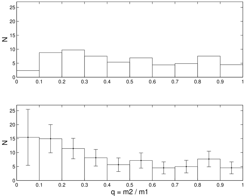
Figure 9: The derived mass ratio distribution plotted as a function of $q$. Top panel: The sum of the mass ratio distributions in the three panels of Figure 8. This is our estimate of the directly measured mass ratio distribution of our sample; it should be reliable above $q\sim 0.3$. Bottom panel: The distribution of the top panel, corrected for binaries undetected in the original L02 sample (see text). The corrections are important below $q\sim 0.3$.

The lowest panel of Figure 8 shows our best estimate of the distribution of the 19 SB1s that remain in our sample, derived by the algorithm of Mazeh & Goldberg (1992), assuming random orientations of the binaries. We did not use the fact that the IR observations could reliably detect a binary with mass ratio larger than $q\sim 0.5$. It is satisfying that the derived distribution is consistent with this limit. It is interesting to compare this estimated distribution with that of the $q_{min}$’s of the same sample (middle panel of Figure 7d). The two are not very different. This is probably because all the systems with small inclinations, and therefore with high mass ratios, were turned into SB2s by our technique, and subsequently were moved to the middle panel of the figure. Thus, the binaries with undetected secondaries have on the average only slightly higher mass ratios than their minimum values. The top panel of Figure 9 shows the sum of the three distributions of Figure 8. This is an estimate of the directly measured mass ratio distribution.

To complete the analysis, we must correct the distribution at the top of Figure 9 for the binaries undetected by L02 and G02. Binaries could have escaped detection because their primary velocity semi-amplitude, $K_{1}$, fell below a certain threshold. For a given sample of binaries with random orientations, this observational selection effect primarily affects binaries with small mass ratios, and so evidently biases the measured distribution (Mazeh, Latham, & Stefanik 1996). The correction Mazeh et al. suggest relies on the assumption that the mass ratio and period distributions are independent, and strongly depends on the period distribution of the sample, because the effect is much stronger for longer periods. However, the observed period distribution of the sample is subject to the same effect, and therefore cannot be used to estimate the true period distribution (e.g., Halbwachs et al. 2003). Thus, although the selection effect is certainly there, the algorithm to correct for it includes inherently large uncertainties.

We corrected for the undetected binaries with the algorithm presented by Mazeh, Latham, & Stefanik (1996), following G03 by assuming a period distribution which is linear in log $P$ with the same parameters. We further assumed that the $K_{1}$ detection threshold is 2.5 km s^-1. The lower panel of Figure 9 presents our result; the uncertainties are given by Poisson statistics, and do not include the systematic errors. As expected, this distribution shows that the effects of the correction are most important below $q\sim 0.3$. For concreteness, we refer to this as the corrected mass ratio distribution.

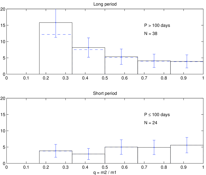
Figure 10: The mass ratio distribution of the short and the long period binaries in our sample.

Halbwachs et al. (2003) suggested that the mass ratio distribution is different for the short and the long period spectroscopic binaries. Trying different periods, they found the best period to separate their sample into short and the long periods is 50 days. We searched for such a difference in our data following Halbwachs et al. approach. Our analysis indicated that if such an effect does exist in our data, it is most pronounced when the sample is divided by a period limit of 100 days. The resulting subsamples include 38 and 24 long and short period binaries, respectively. The resulting mass ratio distributions are depicted in Figure 10.

The two subsamples are smaller than the united sample, and consequently their numerical noise is much larger. Therefore, we derived the two distributions with only six bins. Further, we omitted the first bin in the plot because its uncertainty in the long period subsample is too large to allow any significant comparison. The comparison between the five plotted bins suggests that the mass ratio distribution of the long period binaries rises towards low mass ratio, while the distribution of the short period binaries does not. However, the small sample size and hence large uncertainties in the low-q bins does not allow us to establish this finding firmly, and we need more binaries to investigate the possible difference.

6 Comparison with Previous Studies

Both mass ratio distributions shown in Figure 9, the directly measured one (top panel) and the one corrected for undetected binaries (lower panel), are approximately flat between $q=1$ and $\sim 0.3$. This result appears to differ from the recent derivations of the mass ratio distribution obtained by Halbwachs et al. (2003) and Tokovinin (2000), and is slightly different from the results of G03.

G03 analyzed the whole sample of SBs found in the CL94 survey, and suggested that the mass ratio distribution of the Galactic disk binaries rises monotonically toward low $q$’s. Their Figure 6 (right panel) shows, however, that the rise could be confined to $q<0.3$, and that the distribution is consistent with having an approximately constant value between $q=0.3$ and 1. The Galactic disk sample of G03, consisting of 73 binaries, is very similar to ours, as both were chosen from the CL94 survey. Their sample is somewhat larger, as they did not exclude binaries with distances larger than 90 pc. On the other hand, we added the information about the mass ratio for an additional 32 binaries. Therefore, the flatness of the distribution of the CL94 Galactic disk sample down to $q\sim 0.3$ seems firm from our results. We suggest that the insignificance rise of the distribution in the mass ratio range of 0.3–0.5 indicated by the analysis of G03 is the result of the inherently low resolution of the analysis. This is caused by the lack of mass ratio information for most of the binaries, which can not be recovered by the statistical analysis.

Halbwachs et al.’s (2003) mass ratio distribution shows a prominent peak near $q=1$. This feature confirms the Tokovinin (2000) study, which found a large excess of “twin binaries” in the range of $q$ between $0.95$ and 1. Both studies found this excess to be confined to binaries with periods shorter than 30–50 days. Tokovinin’s sample of SB2s with periods between 2 and 30 days included only 5 systems in the mass ratio range of 0.8–0.9 and 41 binaries in the range of 0.9–1, an enhancement of a factor of $\sim 8$. We do not find such a peak, neither in our Figure 9, which presents our best estimate for the mass distribution of the whole sample studied here, nor in Figure 10, which separates our sample for short and long period binaries.

Tokovinin (2000) studied a sample of published SB2s, detected by different spectrographs and observers. The sample includes the SB2s listed in the Eighth Catalog of Spectroscopic binaries (Batten et al. 1989) and the SB2s included in his compilation of orbits published since then. All the binaries were detected either by direct measurements of the secondary lines, or by resolving the two spectra with the one-dimensional correlation function.

The ability to detect the secondary is sensitive to the light ratio of the primary and the secondary, which in turn strongly depends on the mass ratio. For example, many of the binaries compiled by Tokovinin (2000) were detected by the CfA spectrograph which operates in the visible light, centered at 5200 Å. At this band the stellar luminosity, $L_{5200}$, depends on mass as $L_{5200}\propto M^{\sim 7.4\pm 0.6}$ (G02). Therefore, at q=0.85, for example, the light ratio falls down to $\sim 0.3$, a value that makes the detection of the secondary velocity difficult, depending on the S/N and resolution of the spectra. The fact that Tokovinin’s sample includes a few SB2s with $q\sim 0.8$ does not exclude a strong selection effect against finding such binaries. Those binaries could have been observed with exceptionally high S/N ratio, so that their secondary could have been detected. Tokovinin (2000) noted that his sample could have also included the Öpik effect. We suggest that the high peak at $q\sim 1$ in Tokovinin’s study could be the result of a the combination of the two selection effects. The absence of a similar peak in Tokovinin’s sample for the long-period sample could have arisen in the intrinsic difficulty of resolving the two sets of lines in the spectra of the long period binaries.

We now consider whether our sample could have suffered from an opposite selection effect that prevented us from detecting binaries with $q$ between 0.95 and 1. We could have missed such systems if L02 did not identify binaries with mass ratios close to unity in the original survey for binaries in the sample of high-proper-motion stars. L02 observed all stars in that sample a few times and carefully examined the one-dimensional correlation function of the measured spectra. To escape detection by the L02 survey a binary had to fulfill two conditions. First, the one-dimensional correlation function must not resolve the two set of lines, which can happen only for binaries with small radial velocity amplitude. Second, the radial velocity of the single, blended peak of the correlation must not vary. The blended peak represented the spectral lines of the primary and the secondary together, and therefore was sensitive to the radial velocities of both spectra. Thus, the center of this peak would not vary only if the contribution of the variation of the primary was canceled out by the secondary. This could happen if the light ratio and the radial velocity of the primary and the secondary were the same, possible only in a very narrow range of mass ratios, between, say, $q=0.98$ and unity.

In fact, there is a way to detect some binaries in this range of mass ratios, as Halbwach’s et al. (2003) noted. One could search for the variation of the width of the peak of the one-dimension correlation. Halbwachs et al. (2003) did not include such “line width spectroscopic binaries” in their analysis, because they considered that “the derivation of their orbital elements are rather hazardous”. The result, they commented, is a mass ratio distribution which is biased against twin binaries.

L02, however, have scrutinized carefully the one-dimensional correlation functions for peaks with variable widths, in order to detect binaries hidden by this effect. Once a system with a variable width of the one-dimensional correlation peak was detected, L02 and G02 thoroughly analyzed such systems with TODCOR to try to resolve the two velocities. Obviously, some binaries with mass ratio between, say, $q\sim 0.98$ and 1 and a small radial velocity amplitude could have escaped L02 scrutiny. However, this effect would be the strongest in long period binaries, in contrast to Figure 10, which does not show the twin binary feature for both subsamples. We therefore suggest that the effect in our sample is small and could not explain the discrepancy between our results and those of Tokovinin (2000).

The peak at $q\sim 1$ measured by Halbwach’s et al. (2003) is much smaller than that of Tokovinin’s sample. Halbwach’s et al. Figure 7a suggests that the mass ratio frequency at the peak is higher by a factor of $2.7\pm 0.7$ than the averaged frequency in the range of 0.2–0.9. This peak is based in part on the correction for the line width spectroscopic binaries not included in their analysis. Without the correction, the peak is only 1.4 higher than the averaged frequency. This peak is still not consistent with our results, but the difference is not very significant. Apparently, a much larger sample in needed to establish whether this peak is real or not.

7 Discussion

The main result of our analysis is the flatness of the mass ratio distribution between $q=0.3$ and $1$. Between $q=0.1$ and $0.3$ the distribution might be higher than its value at $q>0.3$, consistent with the peak found by G03 at $q\sim 0.2$. However, the height of the possible rise cannot be determined with confidence, because the uncertainty of the correction at low mass ratios is large and depends on the true distribution of periods in the sample. For example, if we had assumed a flat distribution in $P$ rather than one flat in $\log P$, the correction would have been larger, and the peak at low q’s more prominent. A determination of the mass ratio distribution below $q\sim 0.3$ will require a radial velocity survey with sensitivity better than the CL94 one (L02, G02). We find some evidence that this peak is confined to the binaries with periods longer than 100 days. Below $q=0.1$ our results are very uncertain.

The flatness of the mass ratio distribution between $q=0.3$ and $1$ can already put some constraints on the binary formation models. For example, Bate, Bonnell & Bromm (2002) suggested that a high frequency of close binaries can be produced through a combination of dynamical interaction in unstable multiple systems and orbital decay of initially wider binaries. Orbital decay may occur as a result of gas accretion and/or the interaction of a binary with its circumbinary disc. They found that such mechanisms result in a preference for close binaries to have roughly equal-mass components, a tendency that is not found by our results. On the other hand, dynamical disintegration of small clusters of stars could result in very different mass ratio distributions, depending on the exact parameters of the dynamical model used (Durisen, Sterzik, & Pickett 2000). Durisen, Sterzik, & Pickett (2001) found one model which produced for G type primaries almost flat distribution.

To place our findings in a wider context, we consider the distribution of the masses of the secondaries in our sample. For a sample as homogeneous as ours, the distribution of mass ratios reflects that of secondary masses. Using the median primary mass of 0.72 M_⊙, our result indicates a secondary mass spectrum that is approximately flat down to 0.2 M_⊙, and possibly higher between 0.07–0.2 M_⊙. This differs from the monotonic rise toward low masses found in the single star Initial Mass Functions (IMFs) of young open clusters (e.g., Barrado y Navascues 2002; Tej et al.  2002; Moreaux et al. 2003) and the much younger star forming regions (Luhman et al. 2000). It also differs from the log-normal IMF derived by Chabrier (2003) for the galactic field stars. Our results show that the secondaries in binaries with periods $P<3000$ days are not captured from a single-star IMF, and that their formation mechanisms must differ from that for single stars.

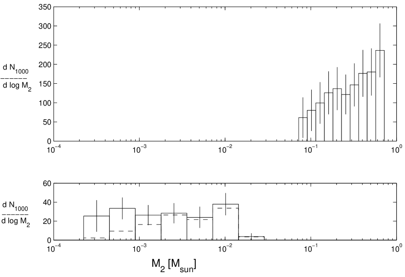
Figure 11: The mass distribution of the stellar secondaries and the extra-solar planets. Both panels give the number of companions for a sample of 1000 single (some of which are multiple) stars per logarithmic unit of secondary mass (see text). The top panel is based on the present work, which is insensitive below 0.07 M_⊙. The bottom panel is based on the present compilation of the published planets (dashed line) corrected for the undetected planets (solid line). The scales of the two panels are different.

It is interesting to compare the distribution of the masses of stellar secondaries with that of the extra-solar planets. In order to compare the two distributions we need to scale their respective parent samples to ones of same size. The binaries studied in this work are found in a set of 488 disk stars closer than 90 pc within the larger CL94 sample. The size of the parent sample of the extra-solar planets is not known. We assume, somewhat arbitrarily, that the planets came from a parent sample of 2000 stars. We scaled both to a common sample size of 1000. The results are shown in Figure 11; the top panel plots the secondary mass distribution of our sample, and the lower panel the mass distribution of the extra-solar planets, both on a logarithmic scale in mass. The scale of the ordinate in both panels is $dN_{1000}/d\log M_{2}$, where $N_{1000}$ is the cumulative number of secondaries up to $M_{2}$ for a parent sample of 1000 single (and multiple) stars. We plotted the secondary distribution down to 0.07 M_⊙, which corresponds to $q=0.1$; our measurements are very insensitive below this value. (While Figure 9 presents number of binaries per mass ratio bin, Figure 11 gives the number per log $M_{2}$ increment.)

To calculate the mass distribution of the extra-solar planets, we used the compilation of the 101 planets as of April, 2003, and applied the MAXLIMA algorithm of Zucker & Mazeh (2001), which derives the distribution of masses from their minimum values, the values actually measured. Following Zucker & Mazeh, we assumed that the population of planets is complete for those with velocity semi-amplitude greater than 40 m s^-1. We therefore used in our analysis only the 70 planets around G and K primaries, with $K_{1}$ larger than this threshold, and corrected the distribution accordingly. The dashed line shows the uncorrected distribution. The uncertainties of the corrected distribution represent the random errors, derived with Monte-Carlo simulations. They do not represent the systematic errors that might be the consequence of the assumed period distribution or even the basic assumption of the independence of the mass and period distributions (e.g., Zucker & Mazeh 2002). The scale of the two panels is different because we find that the frequency of stellar secondaries in the 0.07–0.7 M_⊙ range, with $P<3000$ d, is substantially larger than the presently detected frequency of extra-solar planets in the 1–10 Jupiter mass ($10^{-3}$–$10^{-2}$ M_⊙) range. The former is about 15%, whereas the latter is about 3%, assuming a parent sample of 2000 stars.

The two panels suggest the presence of two distinct populations. Plotted on a logarithmic basis in mass, the stellar secondary population decreases toward the regime of the brown dwarfs. The planetary distribution is consistent with a cutoff above $\sim 15$ Jupiter masses and a flat distribution below this value. The gap separating the two populations is the “brown-dwarf desert” which suggests a natural distinction between a planet and a low-mass stellar secondary based on mass (e.g., Jorissen, Mayor & Udry 2001; Zucker & Mazeh 2001). The decline of the stellar population towards the brown-dwarf region is consistent with the general trends found by Luhman et al. (2000) and Moraux et al. (2003).

8 Closing Remarks

The present analysis of spectroscopic binaries, which relies on combining systematic, precision spectroscopy in visible and IR light, shows that for solar-type main-sequence stars it is already possible to measure the mass ratio distribution in close binaries down to $q\sim$ 0.2–0.3, thereby providing empirical input to theories of binary formation with minimal statistical inference. The prospects are excellent for improving the sensitivity limit to lower mass ratios by analyzing several IR spectroscopic orders simultaneously (Bender et al. 2003).

Purely spectroscopic observations of SB2s, however, leave the orbital inclination, and hence component masses, undetermined. The inclination can be measured by combining the spectroscopic results with interferometric observations that resolve the binary. Boden, Creech-Eakman, & Queloz (2000) have illustrated this approach to derive precise component masses using the Palomar Testbed Interferometer, and Halbwachs et al. (2003) used HIPPARCOS measurements for the same purpose in their study of nearby SBs. The development of ground-based IR interferometers, and the advent of the Space Interferometry Mission, offer the promise of significant progress in this area in the coming decade.

Table 1: Single-Lined Binaries in Sample

System	RA(2000)	Dec(2000)	V	[Fe/H]	d	P	M1,est	$q_{min}$
			(mag)		(pc)	(days)	(M⊙)
G130-32	00:00:03.4	+34:11:22	8.50	-0.58	41	951.00	0.71	$0.16\pm 0.01$
G32-49	00:47:36.5	+14:38:22	10.94	-0.49	77	20.71	0.65	$0.29\pm 0.02$
G173-2	01:30:55.3	+52:44:43	10.05	-0.07	64	339.79	0.79	$0.16\pm 0.01$
G72-58	02:08:23.8	+28:18:38	9.99	-0.55	61	208.0	0.67	$0.23\pm 0.02$
G72-59	02:08:23.8	+28:18:17	10.55	-0.59	61	87.75	0.63	$0.48\pm 0.03$
G173-59	02:33:53.7	+49:30:22	7.75	-0.50	33	2323.00	0.75	$0.62\pm 0.04$
G78-1	02:41:45.7	+47:21:01	9.16	-0.86	67	183.41	0.73	$0.14\pm 0.01$
G77-56	03:29:18.6	+01:58:31	10.45	-0.43	88	179.00	0.73	$0.26\pm 0.02$
G6-20	03:37:11.0	+25:59:27	7.26	-0.25	37	1.93	0.80	$0.69\pm 0.04$
G248-27	04:56:36.2	+72:57:05	9.89	-0.61	52	7.53	0.66	$0.18\pm 0.01$
G84-39	05:12:45.2	+04:19:16	10.58	-0.77	72	8.66	0.63	$0.48\pm 0.03$
G249-37	06:06:24.6	+63:50:06	8.38	-0.27	26	48.96	0.73	$0.32\pm 0.02$
G87-20	07:03:04.8	+38:08:32	9.45	-0.96	57	85.18	0.66	$0.76\pm 0.06$
G108-53	07:05:04.1	+01:23:50	8.45	-0.68	41	612.0	0.71	$0.69\pm 0.05$
G88-5	07:06:08.1	+18:38:10	10.21	-0.57	76	903.9	0.69	$0.21\pm 0.02$
G88-11	07:10:37.3	+20:26:27	9.09	-0.33	56	352.68	0.79	$0.20\pm 0.01$
G112-54	07:54:34.1	$-$01:24:44	7.43	-0.95	17	451.5	0.62	$0.27\pm 0.02$
G40-5	08:04:34.6	+15:21:51	8.48	-0.07	32	75.88	0.79	$0.19\pm 0.02$
G40-8	08:08:54.3	+24:37:26	9.65	-1.02	54	733.5	0.64	$0.22\pm 0.02$
G9-42	09:00:47.4	+21:27:12	8.80	-0.16	38	120.30	0.77	$0.05\pm 0.01$
G41-34	09:22:46.9	+11:16:18	9.65	-0.20	60	193.82	0.78	$0.15\pm 0.02$
G195-30	09:30:18.7	+52:09:11	9.46	-0.69	69	16.91	0.72	$0.12\pm 0.01$
G58-23	10:49:52.6	+20:29:29	9.96	-1.09	71	1779.00	0.66	$0.66\pm 0.06$
G44-45	10:53:23.7	+09:44:21	10.16	-0.33	64	1837.00	0.71	$0.40\pm 0.03$
G147-36	11:17:14.5	+29:34:13	9.29	-0.61	62	6.57	0.73	$0.59\pm 0.04$
G147-58	11:30:22.3	+35:50:30	9.89	-0.64	74	7.15	0.71	$0.69\pm 0.05$
G59-5	12:13:27.7	+23:15:56	9.40	-0.80	64	2483.00	0.70	$0.43\pm 0.03$
G121-75	12:19:00.7	+28:02:52	8.96	-0.24	46	2161.00	0.78	$0.37\pm 0.03$
G60-47	12:55:15.9	+07:49:57	9.93	-0.48	60	1042.5	0.68	$0.42\pm 0.03$
G14-54	13:28:18.7	$-$00:50:24	7.43	-0.22	30	207.32	0.84	$0.19\pm 0.02$
G62-44	13:31:39.9	$-$02:19:03	7.34	-0.69	17	1189.2	0.65	$0.16\pm 0.01$
G165-22	13:38:01.9	+39:10:41	7.78	-0.23	32	11.58	0.82	$0.09\pm 0.01$
G62-61	13:40:26.9	+02:09:05	8.21	-0.42	48	14.49	0.83	$0.49\pm 0.03$
G255-45	13:56:15.1	+74:42:44	9.72	-0.62	83	1620.7	0.73	$0.20\pm 0.03$
G239-38	15:00:26.9	+71:45:55	6.65	-0.68	18	468.1	0.71	$0.11\pm 0.01$
G15-6	15:04:59.5	+04:05:17	9.87	-0.76	63	265.65	0.67	$0.10\pm 0.01$
G66-65	15:07:46.5	+08:52:47	8.27	-0.89	38	201.71	0.70	$0.06\pm 0.01$
G202-25	15:59:56.3	+45:44:10	11.04	-0.38	88	2727.00	0.69	$0.33\pm 0.02$
G17-22	16:32:51.6	+03:14:45	8.84	-0.88	25	226.21	0.59	$1.36\pm 0.13$
G227-37	18:35:09.3	+63:41;47	8.07	-0.33	45	1730.6	0.84	$0.62\pm 0.04$
G21-20	18:37:58.8	$-$06:48:19	8.34	-0.10	31	21.00	0.79	$0.13\pm 0.01$
G22-7	18:55:52.9	$-$05:44:42	7.46	-0.03	25	52.78	0.84	$0.21\pm 0.01$
G262-14	20:28:27.9	+62:00:52	11.46	-0.93	90	81.20	0.61	$0.74\pm 0.06$
G230-45	20:40:16.8	+54:13:14	11.43	-0.87	88	398.3	0.61	$0.47\pm 0.04$
G262-32	20:59:01.4	+65:02:43	10.73	-0.97	61	52.92	0.61	$0.16\pm 0.01$
G26-38	21:58:45.1	+00:48:35	10.29	-0.29	79	2660.00	0.76	$0.24\pm 0.02$
G18-55	22:32:48.5	+10:24:17	9.35	-0.68	39	2916.00	0.64	$0.63\pm 0.05$
G67-38	22:59:19.4	+12:11:32	8.38	-0.67	44	1623.00	0.73	$0.48\pm 0.03$
G156-75	23:01:51.5	$-$03:50:55	7.43	+0.09	17	468.1	0.81	$0.09\pm 0.01$
G157-21	23:09:04.0	$-$02:33:01	9.27	-0.76	54	1134.00	0.68	$0.23\pm 0.02$
G68-31	23:36:06.0	+18:26:33	7.66	-0.35	28	1810.00	0.76	$0.31\pm 0.02$
G130-10	23:46:09.4	+35:14:37	9.13	-0.27	47	1754.6	0.76	$0.21\pm 0.01$

Table 2: SB2s Identified in Visible Light

System	RA(2000)	Dec(2000)	V	[Fe/H]	d	P	M1,est	$q$
			(mag)		(pc)	(days)	(M⊙)
G69-1	00:32:33.9	+28:11:51	8.72	-0.62	72	2127.82	0.72	$0.93\pm 0.02$
G69-4S	00:36:02.3	+29:59:35	8.46	-0.80	40	35.98	0.67	$0.82\pm 0.01$
G34-39	01:37:25.0	+25:10:04	6.97	-0.51	14	25.21	0.64	$0.78\pm 0.01$
G133-57	01:57:34.7	+42:04:36	9.01	-0.22	64	694.87	0.80	$0.76\pm 0.04$
G37-10	02:53:01.4	+35:38:13	8.38	-0.76	37	28.95	0.63	$0.89\pm 0.01$
G6-26A	03:39:33.5	+18:23:05	8.28	-0.89	31	8.65	0.61	$0.96\pm 0.01$
G59-32	12:40:07.0	+20:48:32	8.98	-0.23	57	31.02	0.75	$0.91\pm 0.01$
G16-9	15:45:52.4	+05:02:26	9.15	-0.88	40	9.94	0.60	$0.82\pm 0.02$
G182-7	17:24:42.4	+38:02:10	8.60	-0.69	36	448.61	0.64	$0.88\pm 0.02$
G209-35	20:32:51.6	+41:53:54	7.08	-0.55	21	57.32	0.65	$0.84\pm 0.03$
G210-46	20:59:55.2	+40:15:31	6.57	-0.40	35	112.55	0.84	$0.85\pm 0.02$

Table 3: Observations and Measured Velocities

System	$T_{obs}$	$v_{1}$	$\sigma$	$v_{2}$	$\sigma$
	(MJD-50000)	(km s-1)	(km s-1)	(km s-1)	(km s-1)
G130-32	1916.7	-29.6	0.1	-33.4	0.5
G32-49	2473.0	-26.4	0.1	+43.6	2.4
G173-2	1916.8	-37.6	0.2
G173-2	2474.0	-38.6	0.1
G173-2	2622.9	-35.8	0.1
G72-58	1916.8	+5.9	0.1
G72-58	2474.1	+12.6	0.1
G72-58	2623.8	+15.7	0.1
G72-59	1916.8	+15.9	0.2	+6.7	1.6
G173-59	1916.8	+4.3	0.1	+11.6	2.1
G173-59	2474.1	-1.3	0.1	+20.3	0.8
G173-59	2622.9	+5.9	0.2
G78-1	1916.8	-16.4	0.1	-5.3	1.4
G77-56	2473.1	+25.9	0.1	+45.3	1.0
G6-20	1916.8	-2.9	0.5	-35.6	0.7
G248-27	1916.8	-37.2	0.1	-64.2	1.4
G84-39	1916.9	+44.3	0.2	+92.9	1.8
G249-37	1916.9	+23.7	0.1	+1.9	1.6
G87-20	1916.9	+57.3	0.2	+72.0	1.3
G87-20	1942.9	+87.6	0.1	+35.2	0.5
G108-53	1942.9	+24.5	0.2	+33.9	1.3
G88-5	1916.9	-68.3	0.3
G88-11	1917.0	-29.5	0.1
G88-11	2032.7	-22.2	0.1
G88-11	2623.1	-28.8	0.1
G112-54	1917.0	+96.1	0.1
G112-54	1917.4	+96.5	0.1
G112-54	2032.8	+108.2	0.1
G40-5	1917.0	+25.6	0.2
G40-5	2623.1	+33.9	0.1
G40-8	1917.0	-46.1	0.2	-37.1	0.9
G40-8	2032.8	-46.9	0.2	-37.1	0.5
G9-42	1917.1	+5.6	0.1
G9-42	2032.8	+5.9	0.1	-42.9	5.3
G9-42	2623.1	+6.8	0.1
G41-34	1918.0	+6.1	0.1	+12.5	2.1
G195-30	1918.0	-44.7	0.2
G195-30	1943.0	-69.9	0.2	+102.0	3.0
G195-30	2624.1	-57.4	0.1
G58-23	1917.1	-8.7	0.2	+16.9	0.8
G58-23	1714.8	-4.7	0.3	+13.1	0.7
G58-23	2032.8	-4.4	0.2	+11.3	0.4
G44-45	1918.0	+65.1	0.2
G44-45	1714.8	+66.8	0.2
G44-45	2032.8	+63.1	0.1
G44-45	2624.1	+58.5	0.1
G147-36	1943.0	+54.5	0.1	+31.9	1.0
G147-36	1915.2	+89.3	0.1	-30.9	0.9
G147-58	1918.1	-47.3	0.1	+37.7	1.7
G147-58	1943.1	-5.4	0.1
G147-58	1714.8	+25.0	0.2
G147-58	2062.8	-59.6	0.1
G59-5	1918.1	-29.1	0.2
G59-5	1714.8	-25.5	0.2
G59-5	2032.8	-27.6	0.1
G59-5	2062.8	-28.2	0.2	-34.4	0.5
G121-75	1714.8	+13.7	0.1	+31.3	1.2
G121-75	2032.8	+14.6	0.1	+28.5	0.8
G121-75	1918.1	+13.6	0.1	+29.1	2.6
G60-47	1918.1	+8.6	0.1	+20.3	1.3
G60-47	2032.8	+12.3	0.1	+14.3	0.6
G14-54	1917.1	-12.9	0.1
G14-54	1714.9	-12.9	0.2	+26.1	1.7
G14-54	2032.9	-5.1	0.1	-14.8	2.1
G62-44	1918.1	-50.2	0.3
G62-44	2032.9	-51.6	0.1	-45.2	1.9
G165-22	1917.1	-33.2	0.1
G165-22	1943.1	-28.7	0.1
G165-22	1714.9	-18.8	0.1
G165-22	2061.9	-20.1	0.1
G165-22	2631.2	-17.6	0.1
G62-61	1917.0	+68.3	0.1	-56.5	0.6
G62-61	1943.1	-0.4	0.1	+56.8	0.7
G62-61	2061.9	+68.3	0.1	-56.5	0.5
G255-45	1943.1	-43.4	0.1
G255-45	2062.8	-49.7	0.2	-5.2	2.4
G239-38	2061.9	-50.9	0.1
G15-6	1943.1	-62.2	0.1	-17.3	1.6
G15-6	2062.8	-58.6	0.1
G66-65	1943.1	-57.3	0.1
G66-65	2062.9	-59.9	0.1
G202-25	2063.0	-1.3	0.1	+2.6	1.5
G17-22	1715.0	-71.9	0.1
G17-22	2062.9	-25.1	0.1	-163.0	1.0
G227-37	1715.0	-15.3	0.1	+5.7	1.6
G227-37	2472.9	+2.7	0.1	-28.1	0.4
G21-20	1715.0	-56.6	0.1
G21-20	2062.0	-41.9	0.1
G21-20	2473.9	-56.5	0.1
G22-7	1715.1	-74.3	0.1
G22-7	2472.9	-84.5	0.1
G262-14	1715.1	-54.4	0.3	-89.1	0.4
G262-14	2474.0	-71.7	0.2	-63.7	0.4
G230-45	1715.1	-88.0	0.2	-64.2	1.6
G230-45	2063.0	-88.1	0.2	-62.5	1.3
G262-32	2063.0	-86.4	0.2	-96.1	0.8
G26-38	2063.1	-11.8	0.1	-8.4	1.6
G26-38	2474.0	-14.3	0.1	+1.1	1.4
G26-38	2629.7	-16.4	0.1	+7.0	2.3
G18-55	1916.7	+18.7	0.1	+31.6	1.5
G18-55	1710.1	+19.2	0.2	+27.2	0.5
G67-38	1916.7	-124.7	0.1
G67-38	2062.1	-125.6	0.1	-115.3	1.2
G67-38	2474.0	-126.7	0.1	-120.4	1.7
G156-75	1715.1	-45.3	0.1	-37.1	1.9
G156-75	2474.0	-42.5	0.1
G156-75	2629.7	-44.3	0.1
G157-21	2473.0	-39.6	0.1
G68-31	1917.7	-25.0	0.1
G68-31	2473.0	-28.8	0.1	-12.6	1.2
G130-10	1916.7	-61.6	0.1	-47.0	1.7
G130-10	2474.0	-55.7	0.1

Table 4: Measured Mass Ratios for Systems in Table 1

System	Nobs	Ndet	$q_{min}$	$q_{orb}$	$\alpha$
G130-32	1	1	$0.16\pm 0.01$	$0.62\pm 0.54$	$0.12\pm 0.01$
G32-49	1	1	$0.29\pm 0.02$	$0.36\pm 0.04$	$0.05\pm 0.01$
G173-2	3	0	$0.16\pm 0.01$
G72-58	3	0	$0.23\pm 0.02$
G72-59	1	1	$0.48\pm 0.03$	$0.65\pm 0.35$	$0.28\pm 0.03$
G173-59	3	2	$0.62\pm 0.04$	$0.62\pm 0.09$	$0.05\pm 0.01$
G78-1	1	1	$0.14\pm 0.01$	$0.43\pm 0.17$	$0.08\pm 0.01$
G77-56	1	1	$0.26\pm 0.02$	$0.50\pm 0.10$	$0.13\pm 0.02$
G6-20	1	1	$0.69\pm 0.04$	$0.78\pm 0.09$	$0.36\pm 0.01$
G248-27	1	1	$0.18\pm 0.01$	$0.42\pm 0.09$	$0.05\pm 0.01$
G84-39	1	1	$0.48\pm 0.03$	$0.55\pm 0.07$	$0.16\pm 0.03$
G249-37	1	1	$0.32\pm 0.02$	$0.43\pm 0.12$	$0.05\pm 0.01$
G87-20	2	2	$0.76\pm 0.06$	$0.94\pm 0.06$	$0.19\pm 0.01$
G108-53	1	1	$0.69\pm 0.05$	$0.63\pm 0.31$	$0.10\pm 0.01$
G88-5	1	0	$0.21\pm 0.02$
G88-11	3	0	$0.20\pm 0.01$
G112-54	3	0	$0.27\pm 0.02$
G40-5	2	0	$0.19\pm 0.02$
G40-8	2	2	$0.22\pm 0.02$	$0.69\pm 0.17$	$0.14\pm 0.01$
G9-42	3	0	$0.05\pm 0.01$
G41-34	1	1	$0.15\pm 0.02$	$0.36\pm 0.28$	$0.06\pm 0.01$
G195-30	3	0	$0.12\pm 0.01$
G58-23	3	2	$0.66\pm 0.06$	$0.76\pm 0.12$	$0.16\pm 0.01$
G44-45	4	0	$0.40\pm 0.03$
G147-36	2	2	$0.59\pm 0.04$	$0.57\pm 0.02$	$0.10\pm 0.01$
G147-58	4	1	$0.69\pm 0.05$	$0.54\pm 0.04$	$0.05\pm 0.01$
G59-5	4	1	$0.43\pm 0.03$	$0.53\pm 0.27$	$0.27\pm 0.02$
G121-75	3	3	$0.37\pm 0.03$	$0.29\pm 0.04$	$0.08\pm 0.01$
G60-47	2	2	$0.42\pm 0.03$	$0.55\pm 0.23$	$0.12\pm 0.01$
G14-54	3	2	$0.19\pm 0.02$	$0.20\pm 0.04$	$0.04\pm 0.01$
G62-44	2	0	$0.16\pm 0.01$
G165-22	5	0	$0.09\pm 0.01$
G62-61	3	3	$0.49\pm 0.03$	$0.59\pm 0.01$	$0.17\pm 0.01$
G255-45	2	1	$0.20\pm 0.03$	$0.18\pm 0.03$	$0.05\pm 0.01$
G239-38	1	0	$0.11\pm 0.01$
G15-6	2	0	$0.10\pm 0.01$
G66-65	2	0	$0.06\pm 0.01$
G202-25	1	0	$0.33\pm 0.02$
G227-37	2	1	$0.62\pm 0.04$	$0.49\pm 0.04$	$0.27\pm 0.01$
G21-20	3	0	$0.13\pm 0.01$
G22-7	2	0	$0.21\pm 0.01$
G262-14	2	2	$0.74\pm 0.06$	$0.68\pm 0.05$	$0.52\pm 0.02$
G230-45	2	2	$0.47\pm 0.04$	$0.44\pm 0.05$	$0.14\pm 0.03$
G262-32	1	1	$0.16\pm 0.01$	$0.71\pm 0.28$	$0.30\pm 0.03$
G26-38	3	3	$0.24\pm 0.02$	$0.30\pm 0.04$	$0.06\pm 0.01$
G18-55	2	2	$0.63\pm 0.05$	$0.52\pm 0.14$	$0.13\pm 0.01$
G67-38	3	2	$0.48\pm 0.03$	$0.70\pm 0.20$	$0.08\pm 0.01$
G156-75	3	0	$0.09\pm 0.01$
G157-21	1	0	$0.23\pm 0.02$
G68-31	2	1	$0.31\pm 0.02$	$0.30\pm 0.07$	$0.06\pm 0.01$
G130-10	2	1	$0.21\pm 0.01$	$0.53\pm 0.15$	$0.06\pm 0.01$

References

- (1) Batten, A.H., Fletcher, J.M., & MacCarthy, D.G. 1989, Publ. DAO 17
- Barrado y Navascues et al. (2002) Barrado y Navascues, D., Bouvier, J.R., Lodieu, N., & McCaughrean, M.J. 2002, A&A, 395, 813
- Ba (02) Bate, M.R., Bonnell, I.A., & Bromm, V. 2002, MNRAS, 336, 705
- Bender et al. (2003) Bender, C., Simon, M., Mazeh, T., Zucker, S., & Prato, L. 2003, in prep.
- Boden et al. (2000) Boden, A.F., Creech-Eakman, M.J., & Queloz, D. 2000, ApJ, 536, 880
- Branch (1976) Branch, D. 1976, ApJ, 210, 392
- Carney et al. (1994) Carney, B.W., Latham, D.W., Laird, J.B., & Aguilar, L.A. 1994, AJ, 107, 2240 (CL94)
- Chabrier (200) Chabrier, G. 2003, ApJ, 586, L133
- Clarke, C.J. (2001) Clarke, C.J. 2001 in The Formation of Binary Stars, IAU Symposium No. 200, eds. H. Zinnecker & R.D. Mathieu, (San Francisco:ASP), p. 346
- Clarke, C.J. (2001) Durisen, R.H., Sterzik, M.F., & Pickett, B.K. 2000 in The Formation of Binary Stars, IAU Symposium No. 200, Poster Proceedings, eds. B. Reipurth & H. Zinnecker , (San Francisco:ASP), p. 202
- DSP (2001) Durisen, R.H., Sterzik, M.F., & Pickett, B.K. 2001, A&A, 371, 952
- Goldberg et al. (2002) Goldberg, D. et al. 2002, AJ, 124, 1132 (G02)
- Goldberg et al. (2003) Goldberg, D., Mazeh, T., & Latham, D.W. 2003, ApJ, 521, 397 (G03)
- Halbwachs (1987) Halbwachs, J.L. 1987, A&A, 183, 234
- Halbwachs et al (2003) Halbwachs, J.L., Mayor, M., Udry, S., & Arenou, F. 2003, A&A, 397, 159
- H (95) Heacox, W.D. 1995, AJ, 109, 2670
- JMU (01) Jorissen, A., Mayor, M., & Udry, S. 2001, A&A, 379, 992
- Laird et al. (1988) Laird, J.B., Carney, B.W., and Latham, D.W. AJ, 95, 1843
- Latham et al. (2002) Latham, D.W. et al. 2002, AJ, 124, 1144 (L02)
- Luhman et al. (2000) Luhman, K. et al. 2000, ApJ, 540, 1016
- LR (79) Lucy, L.B., & Ricco, E. 1979, AJ, 84, 401
- Mazeh et al (1992) Mazeh, T., & Goldberg, D. 1992, ApJ, 394, 592
- Mazeh et al (1996) Mazeh, T., Latham, D.W, & Stefanik, R.P. 1996, ApJ, 466, 415
- Mazeh et al. (2002) Mazeh, T. et al. 2002, ApJ, 564, 1007
- McLean et al. (1998) McLean, I.S., et al. 1998, SPIE, 3354, 566
- McLean et al. (2000) McLean, I.S., et al. 2000, SPIE, 4008, 1048
- Moraux et al (2003) Moraux, E., Bouvier, J., Stauffer, J.R., & Cuillandre, J.-C. 2003, A&A, 400, 891
- Öpik (1923) Öpik, E. 1923, Pub. Obs. Astr. Univ. Tartu, 35, No. 6
- (29) Prato, L. et al. 2002a, ApJ, 569, 863
- (30) Prato, L. et al. 2002b, ApJ, 579, L99
- Tej, A. (2002) Tej A., Sahu, K.C., Chandrasekhar, T., & Ashok, N.M. 2002, ApJ, 578, 523
- Tohline (2002) Tohline, J.E. 2002, ARAA, 40, 349
- Tok (2000) Tokovinin, A.A. 2000, A&A, 360, 997
- Udry et al. (2002) Udry, S., Mayor, M., Arenou, F., & Halbwachs, J.L, 2003, in preparation
- ZM (94) Zucker, S., & Mazeh, T. 1994, ApJ, 420, 806
- ZM (01) Zucker, S., & Mazeh, T. 2001, ApJ, 562, 1038
- ZM (02) Zucker, S., & Mazeh, T. 2002, ApJ, 568, 113