The Formation of Broad Emission Line Regions in Supernova-QSO Wind Interactions II. 2D Calculations

One aspect of supernova remnant evolution that is relatively unstudied is the influence of an AGN environment. A high density ambient medium and a nearby powerful continuum source will assist the cooling of shocked ejecta and swept-up gas. Motion of the surrounding medium relative to the remnant will also affect the remnant morphology. In an extension to previous work we have performed 2D hydrodynamical calculations of SNR evolution in an AGN environment, and have determined the evolutionary behaviour of cold gas in the remnant. The cold gas will contribute to the observed broad line emission in AGNs, and we present preliminary theoretical line profiles from our calculations. A more detailed comparison with observations will be performed in future work. The SNR-AGN interaction may be useful as a diagnostic of the AGN wind.

1 Introduction

Active galaxies produce prodigious luminosities in tiny volumes, display very strong cosmological evolution, and are known for the diversity of their behaviour (e.g., Osterbrock & Matthews OM1986 (1986)). Their activity arises from the release of gravitational energy from accretion onto a supermassive ($\sim 10^{6}-10^{9}\hbox{${\rm\thinspace M_{\odot}}$}$) black hole and/or the cumulative effects of short-lived episodes of nuclear star formation, and is often accompanied by nuclear winds and jets. There is evidence (e.g., Williams & Perry WP1994 (1994)) that intense star formation and nuclear activity are related, and starbursts are one possible way to fuel the central black hole. In turn, the nuclear wind and the extreme radiation field act back on the starburst components, influencing stellar winds (and thus stellar evolution), wind blown bubbles, and supernova remnants. For the most luminous active galactic nuclei (AGNs) to be powered by accretion requires that the density of the interstellar medium be enhanced, for example by galaxy encounters or mass loss from a dense nuclear stellar cluster. One of the most important questions concerning the AGN phenomenon is therefore the connection between starburst and nuclear activity.

A defining characteristic of AGNs are their possession of strong (and often very broad) line emission. This provides detailed information on the physical conditions right down into the AGN core, and over the years a great deal has been learned about the properties of the gas comprising the broad emission line region (BELR). It is photoionized, since reverberation studies (e.g., Clavel et al. C1991 (1991)) show the direct response of emission line strengths to continuum variability. The absence of deep Ly$\alpha$ absorption indicates that the BELR covers only $5-25$% of the continuum source (e.g., Bottorff et al. BKSB1997 (1997)). It has a small volume filling factor $\sim 10^{-7}$ (as determined from the observed line strength to continuum ratio; Netzer N1990 (1990)). It also generates a wide range of line profile shapes (indicating that the geometry and kinematics are complex and varied), and shows evidence of at least a two-component structure (Collin-Souffrin et al. CDT1982 (1982), CDJP1986 (1986); Wills et al. WNW1985 (1985)). One of these components is associated with high ionization lines, including C iii], C iv, and other multiply ionized species, and is known as the HIL. The second component can be identified with the low ionization lines which include the bulk of the Balmer lines, and lines of singly ionized species (e.g., Mg ii, C ii, Fe ii) and is known as the LIL.

The regions emitting the LIL and HIL display different kinematics, as deduced from studies of the profiles and line widths (e.g., Gaskell G1988 (1988); Sulentic et al. S1995 (1995)), and the HIL are systematically blue-shifted with respect to the LIL (see, e.g., Sulentic et al. SMD2000 (2000)). To account for the variability of the low ionization Mg ii and Balmer lines the LILs must be optically thick (e.g., Ferland et al. F1992 (1992)). On the other hand, optically thin gas may account for the Baldwin effect (a negative correlation between the ultraviolet emission-line equivalent width and continuum luminosity), although it remains to be seen if this is due to sample biases (Sulentic et al. SMD2000 (2000)), and for the Wamsteker-Colina effect (a negative correlation between between the C iv $\lambda$1549/Ly$\alpha$ ratio and continuum luminosity; Shields et al. SFP1995 (1995)).

It is now fairly clear that the Balmer lines form at the surface of an accretion disk, or close to the surface in an accretion disk wind (e.g., Collin-Souffrin et al. CDMP1988 (1988); Marziani et al. M1996 (1996); Nicastro N2000 (2000)), and approximately three quarters of the total luminosity of the broad-line emission is estimated to arise in the LILs (Collin-Souffrin et al. CDMP1988 (1988)). The geometrical distribution and kinematics of the HIL gas is, however, much less clear: it may arise in a spherical outflow, but a biconical ‘jet-like’ distribution is another possibility. BELR size determinations are commonly obtained using reverberation and photoionization techniques, though it was concluded in a recent study that gravitational microlensing could be a useful alternative method, particularly for the HILs (Abajas et al. AMMPO2002 (2002)).

Many theoretical explanations have been proposed for the origin of the BELR. They include: i) magnetic acceleration of clouds off accretion discs (Emmering et al. EBS1992 (1992)); ii) the interaction of an outflowing wind with the surface of an accretion disc (Cassidy & Raine CR1996 (1996)); iii) interaction of stars with accretion discs (Zurek et al. ZSC1994 (1994)); iv) tidal disruption of stars in the gravitational field of the BH (Roos R1992 (1992)); v) interaction of an AGN wind with supernovae and star clusters (Perry & Dyson PD1985 (1985); Williams & Perry WP1994 (1994)); vi) emission from accretion shocks (Fromerth & Melia FM2001 (2001)); vii) ionized stellar envelopes (e.g.Torricelli-Ciamponi & Pietrini TP2002 (2002)). Many other models have been shown to possess serious difficulties (see references in Pittard et al. PDFH2001 (2001)): in particular, any model must overcome the ‘confinement problem’, and/or continually generate clouds.

Many of the mechanisms on which the various models are based will probably contribute to the production of the observed BELR gas. However, it is clear that some of the proposed mechanisms will be more dominant than others, at least under certain conditions. For example, the rate of tidally disrupted stars in high luminosity AGNs is likely to be too low to account for much of the BELR in these objects. Which are generally the dominant contributions remains, to date, largely unknown.

Even if the SNR-AGN wind interaction is not the dominant formation mechanism of the HIL gas, it is of interest due to its potential as a diagnostic of the AGN wind. Supernovae must occur close to the central AGN engine - in our own Galaxy there exists a cluster of a few dozen evolved massive stars with initial masses $M>20\hbox{${\rm\thinspace M_{\odot}}$}$ (see Figer & Kim FK2002 (2002) and references therein) in a region of 1.6 pc diameter centered on Sgr A*. Recent absorption line measurements from one of the high velocity stars are consistent with an O8-B0 dwarf with a mass $\sim 15\hbox{${\rm\thinspace M_{\odot}}$}$ and a highly eccentric orbit which brings it within 1900 AU ($\approx 6.3\times 10^{-4}{\rm\thinspace pc}$) of the supermassive black hole (Ghez et al. G2003 (2003)). We can expect a similar, if not more extreme, situation in the central regions of AGN.

The evolution of SNRs in a high density static ambient medium has been studied by Terlevich et al. (TTFM1992 (1992)), with particular application to the formation of BELRs in starburst models developed to obviate the existence of supermassive black holes in the centres of AGNs. More recently, the additional influence of an intense continuum radiation field on the evolution of SNRs has been examined (Pittard et al. PDFH2001 (2001)). With Compton cooling and heating processes included in these calculations, the powerful flux of ionizing radiation influences the thermal evolution of shocked regions. A central finding was that shocked gas could radiate efficiently enough to cool to temperatures and densities appropriate for the HIL.

In this paper we present calculations which extend the work of Pittard et al. (PDFH2001 (2001)). We describe the results of 2D axisymmetric hydrodynamical models of the interaction of an AGN wind with a supernova remnant. As the formation, evolution, and structure of cold gas is of particular interest, we have determined the mass of cool gas as a function of time and present some simple modelling of line profiles. In a future paper, we will perform more detailed line profile modelling and will compare the results closely to observations.

In Sec. 2 we discuss the details of our calculations; in Sec. 3 we discuss our results; in Sec. 4 we present some preliminary line profile modelling; and in Sec. 5 we summarize and discuss future work.

2 Details of the calculations

We performed our calculations with an adaptive grid hydrodynamical code which is second order accurate in space and time (see, e.g., Falle & Komissarov FK1996 (1996), FK1998 (1998)). We used a Chevalier-Nadyozhin similarity solution specified by $n=12$, $\delta=0$ as the initial profile for the SNR (Chevalier C1982 (1982); Nadyozhin N1985 (1985)). In the majority of our calculations we assumed a canonical explosion energy of $10^{51}$ ergs and ejecta mass of $10\hbox{${\rm\thinspace M_{\odot}}$}$, which is typical of a type II SN. 75 per cent of the mass and 58 per cent of the explosion energy are contained within a constant density core. Heating and cooling rates for a canonical AGN spectrum were kindly supplied by Tod Woods (cf. Woods et al. W1996 (1996)) and are included in our calculations. They are valid in the optically thin, low-density regime with solar abundances. Further details and assumptions can be found in Pittard et al. (PDFH2001 (2001)) and references therein.

The thermal equilibrium of gas irradiated by the intense continuum in an AGN may be described in terms of several ionization parameters. When cold and hot phases exist with comparable pressure, it is convenient to use a definition based on the ratio of the ionizing photon pressure to gas pressure (cf. Krolik, McKee & Tarter KMT1981 (1981)):

$$\Xi=\frac{1}{4\pi r^{2}nckT}\int_{\nu_{\rm L}}^{\infty}L_{\nu}d\nu,$$ (1)

where $r$ is the distance to the central continuum source, $n$ is the gas density, $T$ the gas temperature, $L_{\nu}$ the differential luminosity, $\nu_{\rm L}$ the frequency at the Lyman limit, and the other symbols have their usual meanings. Another common definition is the ratio of the ionizing photon density to the gas density,

$$U=\frac{1}{4\pi r^{2}nc}\int_{\nu_{\rm L}}^{\infty}\frac{L_{\nu}}{h\nu}d\nu.$$ (2)

The relation between these two ionization parameters depends on the shape of the ionizing spectrum. For the canonical AGN spectrum in Cloudy (see Woods et al. W1996 (1996)), which we adopt for this work,

$$U=0.0182T_{4}\Xi,$$ (3)

where $T_{4}$ is the gas temperature in units of $10^{4}$K. Comparison with Roos (R1992 (1992)) shows that our adopted spectrum is neither particularly soft or hard.

In Figure 1 we show the thermal equilibrium curve for the assumed AGN spectrum as a function of temperature and ionization parameters, $\Xi$ and $U$. At low temperatures photoionization heating and cooling due to line excitation and recombination are in near balance. At high temperatures, the equilibrium arises from the balance of Compton heating and cooling. The exact shape of the thermal equilibrium curve at intermediate temperatures is a complicated function of the irradiating spectrum, the assumed abundances and thermal processes (cf. Krolik et al. KMT1981 (1981)), and varies substantially from source to source. Since we are not modelling a specific object, we do not concern ourselves with the details of this part of the equilibrium curve.

Figure 1: Thermal equilibrium curve for the standard AGN spectrum in Cloudy (see Woods et al. W1996 (1996)).

To obtain cool gas in thermal equilibrium we require ionization parameters $\Xi\mathrel{\hbox to0.0pt{\lower 3.0pt\hbox{$\sim$}\hss}\raise 2.0pt\hbox{$<$}}10$. As noted by Perry & Dyson (PD1985 (1985)), shocked gas cooled back to equilibrium can have a value of $\Xi$ much lower than its pre-shock value. This is because the post-shock density and pressure can be much greater than the pre-shock value. Therefore, strong shocks can create conditions for the gas to cool to temperatures much lower than the surrounding ambient temperature. The crucial question is whether the shocked gas remains at high densities and pressures for long enough to cool from its post-shock temperature to $T\sim 2\times 10^{4}$ K. In our earlier 1D work (Pittard et al. PDFH2001 (2001)) we demonstrated that this was possible for a supernova in a characteristic AGN environment.

In the next section we present results from 2D simulations of a SNR evolving in an AGN environment. We have computed models with ambient densities $n=10^{5},10^{6}\hbox{${\rm{\rm\thinspace cm}^{-3}\,}$}$ and with AGN wind speeds $v=0,3000,5000,7000\hbox{${\rm{\rm\thinspace km}{\rm\thinspace s}^{-1}\,}$}$. The initial radius, expansion speed, and age of the SNR in our models is specified in Table 1 for each of the ambient densities. All models have the same ionization parameter and temperature for the ambient medium ($\Xi\approx 150$, $T=1.33\times 10^{7}$ K) unless otherwise stated. We further assumed that the central continuum source is distant enough that the flux of ionizing radiation is constant over our computational volume. The SNR was evolved until the pressure of the shocked gas drops to the point where it is no longer able to exist in the cool phase ($T\sim 10^{4}$ K). As the remnant expands we periodically regrid our model to a coarser set of grids.

Table 1: Initial radius, $R$, expansion speed, $v_{\rm exp}$, and age, $t$, of the SNR for models with $E=10^{51}$ erg and $M=10\hbox{${\rm\thinspace M_{\odot}}$}$, as a function of the ambient density, $n$.

$n(\hbox{${\rm{\rm\thinspace cm}^{-3}\,}$})$	$R(10^{-3}\;{\rm pc})$	$v_{\rm exp}(\hbox{${\rm{\rm\thinspace km}{\rm\thinspace s}^{-1}\,}$})$	$t$ (yr)
$10^{5}$	3.4	11,000	0.3
$10^{6}$	1.2	12,000	0.1

3 Results

3.1 Expansion into a stationary medium

In Figs. 2 and 3 we show the evolution of a SNR expanding into a stationary environment with $n=10^{6}\hbox{${\rm{\rm\thinspace cm}^{-3}\,}$}$. The shocked gas rapidly loses energy, first through inverse Compton scattering, and then through free-free and line cooling, and is compressed into a relatively thin zone with the unshocked ejecta dominating the remnant volume. The shocked gas has a fractional thickness of 0.132 in the adiabatic self-similar solution (Chevalier C1982 (1982); Nadyozhin N1985 (1985)), but at $t=5{\rm\thinspace yr}$ the radiative energy loss has reduced this to just 0.036.

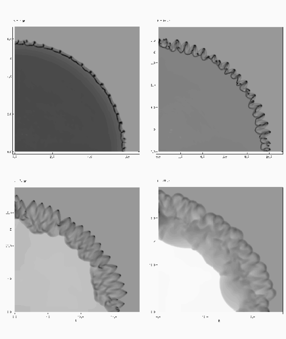
Figure 2: The evolution of a SNR expanding into a stationary environment of density $n=10^{6}\hbox{${\rm{\rm\thinspace cm}^{-3}\,}$}$. Shown are logarithmic plots of the density with a scale from $2.4\times 10^{4}\hbox{${\rm{\rm\thinspace cm}^{-3}\,}$}$ (white) to $3.1\times 10^{8}\hbox{${\rm{\rm\thinspace cm}^{-3}\,}$}$ (black). The age of the remnant is shown in the upper left corner of each plot. Note the change in the axis scaling between the plots. The unit of length in these and subsequent plots is $1.1\times 10^{16}{\rm\thinspace cm}$ (0.0036 pc), and the ionization parameter of the surrounding medium, $\Xi\approx 150$, unless explicitly stated otherwise.

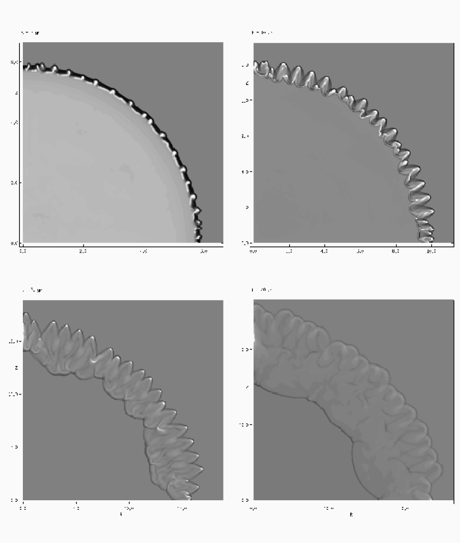
Figure 3: As Fig. 2 but showing logarithmic plots of the temperature with a scale from $10^{6}{\rm\thinspace K}$ (white) to $1.58\times 10^{8}{\rm\thinspace K}$ (black). Note the creation, evolution, and destruction of cool gas ($T<10^{6}{\rm\thinspace K}$) within the remnant.

Since the shocked ejecta are denser than the swept-up gas, they cool quicker and form a thin dense shell within the narrow region of shocked gas, which is bounded on its interior surface by the reverse shock. Since the dense shell is decelerated by the hot gas on its outside surface, it is subject to the Rayleigh-Taylor instability, and there have been many investigations of this behaviour in SNRs (e.g., Chevalier et al. CBE1992 (1992); Chevalier & Blondin CB1995 (1995); Jun et al. JJN1996 (1996); Blondin et al. BBR2001 (2001); Blondin & Ellison BE2001 (2001); Wang & Chevalier WC2002 (2002)).

While previous numerical calculations of remnants in the literature showed that the shocked ejecta were unable to distort the position of the forward shock (the Rayleigh-Taylor (R-T) “fingers” being limited to about half the thickness of the region of hot, swept-up gas; Chevalier et al. (CBE1992 (1992)), a number of exceptions have recently been found. For instance, the existence of circumstellar cloudlets was found to enhance the growth of the R-T fingers by generating vortices in the swept-up gas (Jun et al. JJN1996 (1996)). Alternatively, if the forward shock is an efficient site for particle acceleration, the shock compression ratio is increased and the region of hot, swept-up gas is reduced in thickness, allowing the convective instabilities to reach all the way to the forward shock (Blondin & Ellison BE2001 (2001)). Finally, if the ejecta are clumpy, the greater momentum of the clumps enables them to push through the position of equlibrium pressure balance and to perturb (or puncture) the forward shock (cf. Blondin et al. BBR2001 (2001); Wang & Chevalier WC2002 (2002)).

To this list we can add the present work. In the high density, high radiation flux environment which we consider, the region of swept-up gas is significantly more efficient at radiating energy than in less extreme environments, and is thus more strongly compressed than normal. In this sense our models mimic the higher compression ratios found in models with efficient particle acceleration (Blondin & Ellison BE2001 (2001)), and like them we find that the high density “fingers” are able to distort the forward shock. Chevalier et al. (CBE1992 (1992)) had previously suggested the possibility of a highly radiative inner shock front to explain protrusions seen in VLBI observations of SN 1986J. The large decrease in entropy of the shocked ejecta greatly enhances this instability.

At $t=10{\rm\thinspace yr}$, the R-T “fingers” have grown so long, and distorted the forward shock to such an extent, that the instability begins to resemble the non-linear thin shell instability (hereafter NTSI; Vishniac V1994 (1994)). To our knowledge this has never been seen before in SNRs, although it is a common phenomena in simulations of wind blown bubbles (e.g., García-Segura et al. GML1996 (1996)) and colliding stellar winds (e.g., Stevens et al. SBP1992 (1992); Pittard et al. PSCI1998 (1998)).

We note that the “fingers” do not form at constant intervals along the thin shell. Since they are not deliberately seeded, they naturally develop from noise within the code itself. It is known from both analytical and numerical work that small wavelength modes grow most rapidly for both the R-T instability (Chandrasekhar C1961 (1961); Youngs Y1984 (1984)) and the NTSI (Vishniac V1994 (1994); Blondin & Marks BM1996 (1996)). However, it is extremely difficult to resolve modes of the thin-shell instability, as a sufficient number of grid cells across the thin shell is needed to follow the tangential flow of material (Mac Low & Norman MN1993 (1993)). Given that this is not the case in our models, we expect the development of this instability to differ in higher resolution runs. Nevertheless, we do not expect it to drastically alter the mass of gas that cools (see Section 3.4).

Until about $t=7{\rm\thinspace yr}$, the ejecta envelope impacts the reverse shock, and the pre-shock density remains relatively constant at $n\approx 7\times 10^{6}\hbox{${\rm{\rm\thinspace cm}^{-3}\,}$}$. However, soon after this the reverse shock interacts with the ejecta core. During this stage the ram pressure of the ejecta on the shocked gas rapidly declines as the pre-shock density now decreases as $t^{-3}$, and the shocked region depressurizes as the reverse shock travels towards the center of the remnant. This loss in pressure raises the equilibrium ionization parameter, $\Xi$, of the shocked gas to the point that the equilibrium temperature changes from $\sim 10^{4}{\rm\thinspace K}$ to $\sim 10^{7}{\rm\thinspace K}$. Gas that has managed to cool to $T\sim 10^{4}{\rm\thinspace K}$ is then heated. This behaviour is seen in Fig. 3. At $t=5{\rm\thinspace yr}$ much of the shocked ejecta has cooled to $T\approx 2\times 10^{4}{\rm\thinspace K}$, and at $t=10{\rm\thinspace yr}$, this has significant structure from the action of the instabilities. However, by $t=20{\rm\thinspace yr}$ most of the cool gas has disappeared, with only a few regions concentrated at the densest points of the remnant, these typically being at the extremeties resulting from the “fingers” mentioned earlier. By $t=40{\rm\thinspace yr}$ even these regions have disappeared, and the remnant is at an almost uniform temperature $T\approx 1.3\times 10^{7}{\rm\thinspace K}$.

Remnants expanding into lower density surroundings are characterized by a thicker region of swept up material; those expanding into higher density have a thinner region of swept up material. Fig. 4 shows the morphology of a remnant expanding into a stationary medium with $n=10^{5}\hbox{${\rm{\rm\thinspace cm}^{-3}\,}$}$.

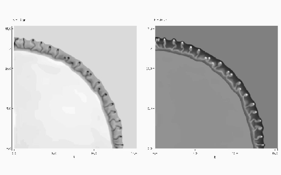
Figure 4: The morphology of a SNR expanding into stationary surroundings with $n=10^{5}\hbox{${\rm{\rm\thinspace cm}^{-3}\,}$}$ at $t=30{\rm\thinspace yr}$. Left: logarithmic density (grayscale from $4.7\times 10^{4}\hbox{${\rm{\rm\thinspace cm}^{-3}\,}$}$ (white) to $1.8\times 10^{7}\hbox{${\rm{\rm\thinspace cm}^{-3}\,}$}$ (black)). Right: logarithmic temperature (grayscale from $10^{6}{\rm\thinspace K}$ (white) to $1.58\times 10^{8}{\rm\thinspace K}$ (black)). The unit of length is $2.24\times 10^{16}{\rm\thinspace cm}$ (0.0073 pc).

3.2 Expansion into an AGN wind

Several major differences in the morphology and evolution of the remnant are seen when it expands into a high velocity flow rather than into a stationary medium. Fig. 5 shows density and temperature plots of a remnant expanding into a flow with $n=10^{6}\hbox{${\rm{\rm\thinspace cm}^{-3}\,}$}$ and $v=3000\hbox{${\rm{\rm\thinspace km}{\rm\thinspace s}^{-1}\,}$}$. Since the expansion velocity of the remnant is intially much higher than this, the flow velocity of the surrounding medium has little effect on the remnant morphology at early times. However, as the expansion velocity of the remnant slows, the flow velocity becomes increasingly significant, and the remnant is distorted from a spherical shape in the way that one would expect. The resulting morphology can be compared to that seen in adiabatic remnants expanding into a plane-stratified (stationary) medium (Arthur & Falle AF1993 (1993)). The models show increasing distortion of the remnant with wind speed.

Motion of the ambient medium also affects the development of hydrodynamic instabilities. On the leading edge of the remnant, instabilities are more vigorous, since the shocked region is compressed to higher densities. On the trailing edge, the shocks are much weaker, and the shocked gas is both less dense and broader in extent, which severely suppresses the activity of the instabilities in this region. Since the trailing edge has relatively low pressure, $\Xi$ is much higher here than at the leading edge, and cool gas forms preferentially in the upstream direction. We find that the evolution of the mass of cool gas is surprisingly similiar over a wide range of ambient densities and flow speeds (see Sec. 3.4).

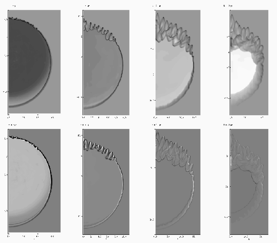
Figure 5: The evolution of a SNR expanding into an AGN wind with $n=10^{6}\hbox{${\rm{\rm\thinspace cm}^{-3}\,}$}$ and $v=3000\hbox{${\rm{\rm\thinspace km}{\rm\thinspace s}^{-1}\,}$}$. In this figure the AGN wind propagates down the page and the explosion site is at position (0,0). The top row shows logarithmic plots of the density with a scale from $2.4\times 10^{4}\hbox{${\rm{\rm\thinspace cm}^{-3}\,}$}$ (white) to $3.1\times 10^{8}\hbox{${\rm{\rm\thinspace cm}^{-3}\,}$}$ (black), while the bottom row shows logarithmic plots of the temperature with a scale from $10^{6}{\rm\thinspace K}$ (white) to $1.58\times 10^{8}{\rm\thinspace K}$ (black). The age of the remnant is shown in the upper left corner of each plot. Note the change in the axis scaling between the plots.

3.3 Individual cool clumps

In the upper panels of Fig. 6 we zoom in on the remnant limb from the simulation at $t=10{\rm\thinspace yr}$ as shown in Figs. 2 and 3. The forward shock bounds the right side of the shocked gas, and the reverse shock bounds the left. The high densities apparent in the upper panels lead to rapid cooling of the post-shock flow, such that the morphology resembles that resulting from the ram-ram pressure instability. The lower panels of Fig. 6 display the remnant limb at $t=30{\rm\thinspace yr}$ for expansion into an ambient density $n=10^{5}\hbox{${\rm{\rm\thinspace cm}^{-3}\,}$}$ (see Fig. 4). Compared to the situation shown in the upper panels the post-shock flow cools far less strongly, and we see that the cool regions are embedded in a much thicker region of shocked gas.

Of note is the fact that the cool regions (which we shall identify henceforth as “clouds”) contain within them a range of densities, equilibrium ionization parameters, and velocities. The clouds, being surrounded by a confining medium, are indeed long-lived: they remain as distinct entities until their pressure drops to the point where their equilibrium temperature corresponds to the hot phase. Within an AGN as a whole where many young SNRs will exist at a given time, cool clouds will be continuously created (through gas cooling in the younger remnants) and destroyed (through gas re-heating in the older remnants).

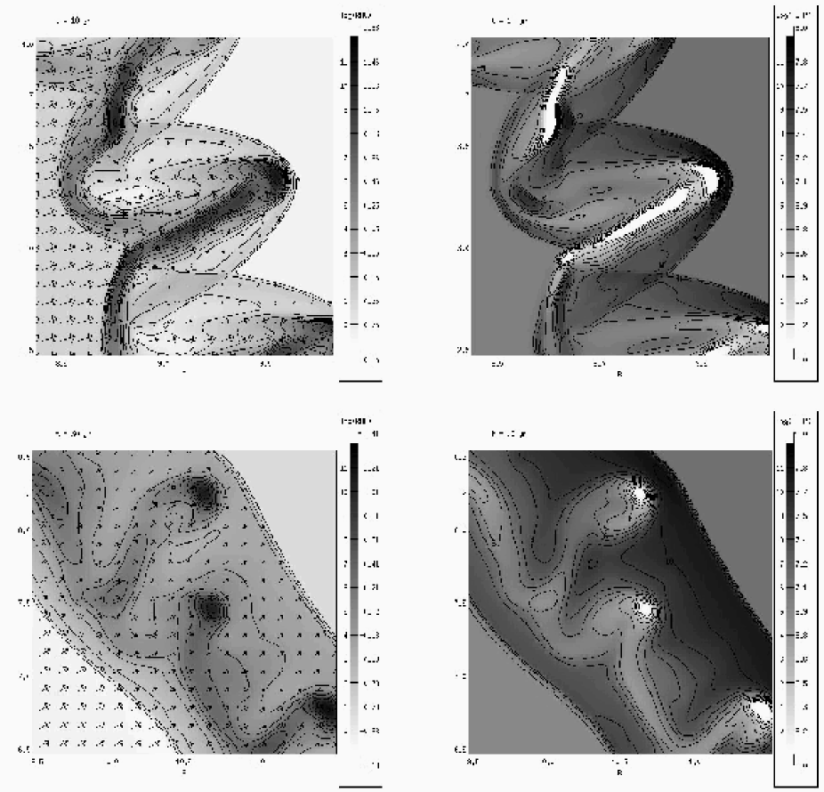
Figure 6: The density and temperature structure of individual bowshocks and cool clumps. The top panels show the structure existing at $t=10{\rm\thinspace yr}$ when a remnant expands into an ambient density $n=10^{6}\hbox{${\rm{\rm\thinspace cm}^{-3}\,}$}$. The bottom panels show the structure existing at $t=30{\rm\thinspace yr}$ when a remnant expands into an ambient density $n=10^{5}\hbox{${\rm{\rm\thinspace cm}^{-3}\,}$}$. The left panels display density gray-scales, contours, and flow vectors, while the right panels display temperature gray-scales and contours.

3.4 Evolution of cool gas

The mass of the cool clouds as a function of time is shown in Figs. 7 and 8, and Table 2. We define $M=\int_{\Xi=0}^{\Xi}M(\Xi)d\Xi$. The first gas to cool below $T=10^{6}{\rm\thinspace K}$ is initially out of pressure equilibrium with its surroundings as the cooling timescale of this gas is shorter than the dynamical timescale of the surrounding material. This can be seen by examining Fig. 7, where during the re-establishment of pressure equilibrium, $\Xi$ decreases. For the remaining evolution, continued expansion of the remnant causes $\Xi$ to increase towards the ambient value ($\Xi\approx 150$). While $\Xi$ is below the value separating the cool and hot phases ($\Xi\approx 30$ - see Fig. 1), gas continues to cool and the total mass of cool gas continues to rise. However, when $\Xi\mathrel{\hbox to0.0pt{\lower 3.0pt\hbox{$\sim$}\hss}\raise 2.0pt\hbox{$>$}}30$, the clouds are subject to net heating, and the mass of cold gas decreases until the clouds are eventually completely destroyed. Fig. 7 shows that not all of the clouds transit from a cool to a hot phase at exactly the same time. Pressure and density enhancements in the remnant caused by the action of instabilities are able to maintain some clouds in their cool phase for a longer duration.

Figure 7: The evolution of cool gas in remnants expanding into a surrounding medium with $n=10^{6}\hbox{${\rm{\rm\thinspace cm}^{-3}\,}$}$. The mass of cool gas with an ionization parameter below $\Xi$ is shown as a function of $t$ for flow speeds of $v=0,\;3000,\;5000,\;7000\hbox{${\rm{\rm\thinspace km}{\rm\thinspace s}^{-1}\,}$}$.

When the surrounding medium is in motion relative to the progenitor of the explosion, the increased compression of the leading edge of the remnant results in cool gas forming more rapidly and with a lower value of $\Xi$. The cool gas is also able to survive for a longer time in such cases. For $n=10^{6}\hbox{${\rm{\rm\thinspace cm}^{-3}\,}$}$, the total mass of cool gas is fairly insensitive to the flow speed of the ambient medium, peaking at $M\sim 2-4\hbox{${\rm\thinspace M_{\odot}}$}$ approximately $15-20{\rm\thinspace yr}$ after the explosion. On the other hand, the increased compression caused by a wind can significantly enhance the mass of cool gas in situations where its formation is otherwise marginal. For example, when $n=10^{5}\hbox{${\rm{\rm\thinspace cm}^{-3}\,}$}$, gas barely manages to cool below $T\approx 10^{6}{\rm\thinspace K}$ when the medium is stationary, but in the model with $n=10^{5}\hbox{${\rm{\rm\thinspace cm}^{-3}\,}$}$ and $v=3000\hbox{${\rm{\rm\thinspace km}{\rm\thinspace s}^{-1}\,}$}$ a substantially greater mass of gas cools and exists for a significantly longer period.

The results of most observational work are reported in terms of the ionization parameter $U$ (Eq. 2). Since we know the relationship between $U$ and $\Xi$ for the AGN spectrum adopted in our models (Eq. 3), we can therefore easily compare our results to observations, where a large range in $U$ is seen. Low ionization lines (such as Mg ii $\lambda 2800$) typically have $U\sim 0.01$, which translates into $\Xi\sim 0.3$ for gas at $T\approx 20000{\rm\thinspace K}$. In contrast, high ionization lines (such as C iv $\lambda 1549$) are characterized by larger values of $U$ - low values of C iii $\lambda 977$/O vi $\lambda 1034$ imply the presence of gas with $U\sim 1$ (Laor et al. L1994 (1994)). This translates into $\Xi\sim 25$ for gas existing in the cool phase, which is clearly in good agreement with the results presented in Fig. 7.

Figure 8: The evolution of the mass of cool clouds in remnants expanding into a surrounding medium with $n=10^{5}\hbox{${\rm{\rm\thinspace cm}^{-3}\,}$}$ (top) and $n=10^{6}\hbox{${\rm{\rm\thinspace cm}^{-3}\,}$}$ (bottom). In each panel the mass of cool gas is shown as a function of $t$ for flow speeds of $v=0,\;3000,\;5000,\;7000\hbox{${\rm{\rm\thinspace km}{\rm\thinspace s}^{-1}\,}$}$.

Table 2: Time evolution of the mass (${\rm\thinspace M_{\odot}}$) of cool clouds in remnants expanding into a surrounding medium with various density, flow speed, and ionization parameter. Columns 2-5 show results for an ambient density $n=10^{5}\hbox{${\rm{\rm\thinspace cm}^{-3}\,}$}$. Columns 6-11 are for an ambient density $n=10^{6}\hbox{${\rm{\rm\thinspace cm}^{-3}\,}$}$. In columns 10 and 11 we give results for stationary surroundings but with either an enhanced AGN flux (causing a 10x increase in the ionization parameter of the ambient medium to $\Xi\approx 1500$), or remnant parameters suitable for a type Ia SN explosion (see Secs. 3.5 and 3.6 respectively). Dashes indicate that no cool gas exists. The bottom row contains values for the integrated area under the mass vs. time curve, in units of $\hbox{${\rm\thinspace M_{\odot}}$}{\rm\thinspace yr}$.

$t({\rm\thinspace yr})$	$n=10^{5}\hbox{${\rm{\rm\thinspace cm}^{-3}\,}$}$				$n=10^{6}\hbox{${\rm{\rm\thinspace cm}^{-3}\,}$}$
	0	3000	5000	7000	0	3000	5000	7000	High $\Xi$	SN Ia
2.5	-	-	-	-	0.0072	0.074	0.11	0.37	-	-
5.0	-	-	0.0015	0.035	0.83	1.1	1.4	1.5	-	-
7.5	-	0.047	0.20	0.42	2.3	2.1	2.4	2.7	-	0.51
10.0	-	0.29	0.31	0.63	2.3	3.2	3.2	2.5	-	0.79
15.0	-	0.46	0.71	1.1	1.5	4.3	2.7	3.7	-	0.30
20.0	0.48	0.77	0.23	0.55	1.3	1.7	3.8	1.8	-	0.033
25.0	0.58	0.84	0.35	0.84	0.91	1.5	3.4	1.7	-	-
30.0	0.54	0.85	0.30	1.1	0.66	0.89	0.33	1.09	-	-
35.0	0.37	0.39	0.32	1.4	-	0.01	0.43	0.77	-	-
40.0	0.095	0.33	0.34	0.27	-	-	0.32	0.53	-	-
50.0	0.056	0.40	-	0.17	-	-	-	0.098	-	-
60.0	-	0.20	-	0.043	-	-	-	0.051	-	-
70.0	-	-	-	0.040	-	-	-	-	-	-
80.0	-	-	-	0.0025	-	-	-	-	-	-
90.0	-	-	-	-	-	-	-	-	-	-
$Mt$	11	26	14	33	39	62	77	71	-	6

3.5 Effect of an increased AGN flux

The simulations shown so far were computed with an AGN flux which was high enough to maintain the ambient gas in the hot phase (i.e. $\Xi\approx 150$ - see the equilibrium curve in Fig. 1). This resulted in a relatively low value of $\Xi$ for the shocked gas and provided a good opportunity for the shocked gas to cool to $T\approx 2\times 10^{4}{\rm\thinspace K}$. However, if a remnant were to be immersed in ambient gas with a higher ionization parameter, the ability for shocked gas to cool would be compromised. This is shown in Fig. 9, where a remnant is expanding into a stationary medium with $\Xi\approx 1500$ (i.e. $\Xi$ is 10x higher than in Figs. 2 and 3). The increased photon flux from the AGN increases the rate of Compton heating, and leads to a reduction in the net cooling rate. While the radius of the remnant is largely unchanged, its morphology is affected: the shocked gas is not compressed as much, and cool clouds do not form. This behaviour is consistent with the earlier work presented in Pittard et al. (PDFH2001 (2001)).

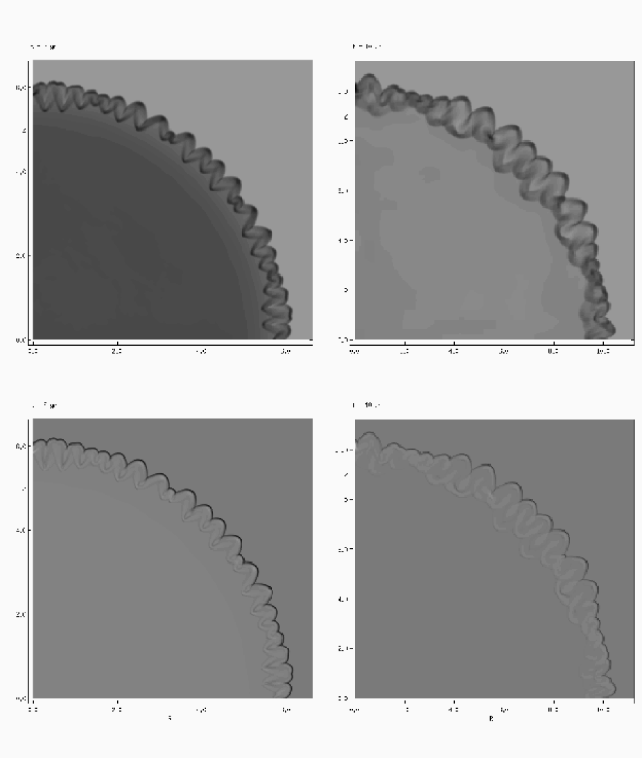
Figure 9: The evolution of a SNR expanding into a stationary environment with $n=10^{6}\hbox{${\rm{\rm\thinspace cm}^{-3}\,}$}$ and $\Xi\approx 1500$. The top panels show logarithmic plots of the density, while the bottom panels show logarithmic plots of the temperature (same scaling as in Figs. 2 and 3). Note that cool clouds do not form in this case.

3.6 Effect of the stellar envelope

To investigate whether cool clouds could form in a remnant from a type Ia SN explosion, we have computed an additional model with appropriate parameters: $E=10^{51}{\rm\thinspace erg}$, $M=1.4\hbox{${\rm\thinspace M_{\odot}}$}$, and $n=7$ (cf. Chevalier C1982 (1982)). The main difference with this model is that the increased value of $E/M$ results in higher expansion velocities of the ejecta and hotter post-shock gas, and a lower equilibrium ionization parameter. However, the remnant also decelerates more rapidly, causing $\Xi$ to increase at a faster rate than for the $n=12$ case. This ultimately hinders the formation of cool gas relative to the $n=12$ case, and only a small amount is able to form (see Table 2).

Recently, it is has become clear that there exists a class of type II supernova explosions which are under energetic (e.g., Zampieri et al. Z2003 (2003)). For two explosions examined in detail, Zampieri et al. (Z2003 (2003)) found $M\mathrel{\hbox to0.0pt{\lower 3.0pt\hbox{$\sim$}\hss}\raise 2.0pt\hbox{$>$}}14\hbox{${\rm\thinspace M_{\odot}}$}$ and $E\approx 0.6-0.9\times 10^{51}{\rm\thinspace erg}$. We do not expect remnants with such parameters to evolve significantly differently to our canonical models with $M=10\hbox{${\rm\thinspace M_{\odot}}$}$ and $E=10^{51}{\rm\thinspace erg}$.

4 Line profiles

We have calculated synthetic line profiles for emission from the cooled gas. The 2D axisymmetric grid is rotated onto a 3D cartesian grid and the emission from volume elements containing cool gas was integrated under the assumption that it is optically thin and the volume emission rate varies as $n^{2}$. Since the gas is cool, thermal Doppler broadening is negligible. A previous investigation (Bottorff et al. BFBK2000 (2000)) failed to reach any strong conclusions concerning whether microturbulence was favoured by observations, so it is not included in our model. The emission is blue- or redshifted according to the line of sight velocity of the gas. Absorption was also assumed to be negligible.

In Fig. 10 we show the line profiles resulting from a remnant expanding into an ambient medium with 3 sets of parameters. The normalization of the line profiles has been set so that the peak emission is approximately 1.0, and we have preserved the relative scaling between the models (e.g., the central intensity of the $n=10^{6}\hbox{${\rm{\rm\thinspace cm}^{-3}\,}$}$, $v=0\hbox{${\rm{\rm\thinspace km}{\rm\thinspace s}^{-1}\,}$}$, $t=20{\rm\thinspace yr}$ profile is approximately $4\times$ greater than the central intensity of the $n=10^{5}\hbox{${\rm{\rm\thinspace cm}^{-3}\,}$}$, $v=0\hbox{${\rm{\rm\thinspace km}{\rm\thinspace s}^{-1}\,}$}$, $t=20{\rm\thinspace yr}$ profile). The bottom row in Fig. 10 shows the line profile which results if we integrate over the age of the remnant. In effect we sum each of the profiles in the rows above with an appropriate weight which reflects the time between each “snapshot”.

Figure 10: Line profiles from cool gas formed in a SNR expanding into an AGN environment with $\Xi\approx 150$ and integrated over many lines of sight (i.e. it is assumed that there is a spherical distribution of remnants in an isotropic medium and radiation field). The left and middle columns are for stationary environments with $n=10^{5}\hbox{${\rm{\rm\thinspace cm}^{-3}\,}$}$ and $n=10^{6}\hbox{${\rm{\rm\thinspace cm}^{-3}\,}$}$, respectively. The right column is for an environment with $n=10^{6}\hbox{${\rm{\rm\thinspace cm}^{-3}\,}$}$ and $v=3000\hbox{${\rm{\rm\thinspace km}{\rm\thinspace s}^{-1}\,}$}$. In the top two rows the line profile at specific remnant ages is displayed, with the age of the remnant (in years) marked next to each profile. The solid line in the top row corresponds to $t=20{\rm\thinspace yr}$ for $n=10^{5}\hbox{${\rm{\rm\thinspace cm}^{-3}\,}$}$, and $t=5{\rm\thinspace yr}$ for $n=10^{6}\hbox{${\rm{\rm\thinspace cm}^{-3}\,}$}$. The remaining profiles in the top and middle rows correspond to the subsequent entries in Table 2, with the line width decreasing with remnant age. In the bottom row the average line profile integrated over the age of the remnant is displayed. Note the difference in the scaling of the intensity axis.

In general, the normalization first rises and then falls with time as cool clouds are created and then destroyed. The width of the line decreases with time as the expansion speed of the remnant slows. The line is clearly flat-topped, which is characteristic of emission from a geometrically and optically thin spherical shell (see, e.g., Fig. 3 in Capriotti et al. CFB1980 (1980) with $v_{\rm min}/v_{\rm max}\approx 1.0$). As the effective thickness of the “shell” in Fig. 2 is minimal, a tangential line of sight does not intercept an increased number of clouds, and “horns” are not seen in the profile. In contrast, the line profiles displayed in the rightmost column of Fig. 10 show an increasingly rounded or triangular profile as the remnant ages, and the time-averaged profile displays a distintly rounded top. In this model the remnant is expanding into an AGN wind and the line profiles (which are sensitive to the spatial distribution of cool gas) reflect the increasing distortion of the remnant as it expands.

It is clear from Fig. 2 that the emission is from a relatively small number of clouds (particularly at later times, e.g., $t=20{\rm\thinspace yr}$). This introduces a great deal of small scale structure into the line profiles which we have smoothed out in Fig. 10 by averaging over many different lines of sight. Observed line profiles from AGN are in reality very smooth, and it has been concluded that the number of emitting clouds must be $\sim 10^{5}$ (Arav et al. A1997 (1997)), although this would be reduced if there was significant microturbulence. Alternatively, electron scattering could help to explain smooth broad line profiles, especially in the line wings (Emmering et al. EBS1992 (1992)). In our 2D hydrodynamical models the clouds are in fact rings, and numerical viscosity and the finite number of grid cells limit the number of distinct clouds which form. Increased numerical resolution and 3D simulations will produce many more distinct clouds, but present limitations mean that the line profiles from our models are not as smooth as seen in observations, and their fine structure should be ignored.

In Fig. 11 we show the line profiles resulting from a remnant expanding into an AGN wind of speed $v=3000,5000$, and $7000\hbox{${\rm{\rm\thinspace km}{\rm\thinspace s}^{-1}\,}$}$, for a viewing angle, $\theta=135^{\circ}$. Here $\theta$ is defined as the angle between the AGN wind vector and the vector from the observer to the remnant (i.e. $\theta=0^{\circ}$ corresponds to the observer facing the side of the remnant expanding into the oncoming AGN wind). Inspection of Fig. 5 reveals that cool clouds exist over a wide range of angles, namely from $\theta=0^{\circ}$ to $\theta\approx 135^{\circ}$. For a line of sight with $\theta=135^{\circ}$ (i.e. where the flow has a velocity component towards the observer), the blue wing of the line shows the greater extension at $t=10{\rm\thinspace yr}$. This is expected since the trailing edge of the remnant is not decelerated as rapidly as the leading edge. However, at $t=5{\rm\thinspace yr}$, the cold clouds exist predominantly on the leading edge (the density and cooling rate are highest here) and it is the red edge of the line profile that is the most extended. This behaviour is also seen when the remnant expands into a flow with $v=5000$ or $7000\hbox{${\rm{\rm\thinspace km}{\rm\thinspace s}^{-1}\,}$}$. Hence as the remnant expands, the resulting line profile flips from a red to a blue-shift (and vice-versa for $\theta\mathrel{\hbox to0.0pt{\lower 3.0pt\hbox{$\sim$}\hss}\raise 2.0pt\hbox{$<$}}45^{\circ}$).

Figure 11: Line profiles from cool gas formed in a SNR expanding into an AGN wind with $n=10^{6}\hbox{${\rm{\rm\thinspace cm}^{-3}\,}$}$, $\Xi\approx 150$, and $v=3000,5000,$ or $7000\hbox{${\rm{\rm\thinspace km}{\rm\thinspace s}^{-1}\,}$}$. The line-of-sight is specified by $\theta=135^{\circ}$ (i.e. there is a component of the AGN wind moving towards the observer) and the profiles are from remnants of age $t=5{\rm\thinspace yr}$ (top row), $t=10{\rm\thinspace yr}$, $t=15{\rm\thinspace yr}$, and $t=20{\rm\thinspace yr}$. In the bottom row the age integrated profiles are shown.

For each of the 3 distinct cases of ambient medium investigated in Fig. 10, the time-averaged line profile displayed in the bottom row has a FWHM $\approx 4500-5000\hbox{${\rm{\rm\thinspace km}{\rm\thinspace s}^{-1}\,}$}$, and a full width at zero intensity of $\approx 6000-8000\hbox{${\rm{\rm\thinspace km}{\rm\thinspace s}^{-1}\,}$}$. This range lies almost in the middle of the distribution of FWHM measures of the broad component of C iv $\lambda 1549$ for radio-quiet sources (Sulentic et al. SMD2000 (2000)).

In Table 3 we list various statistics for the time-averaged line profiles shown in Fig. 11. Radio quiet sources show a scatter in the asymmetry values for the broad component of the C iv$\lambda 1549$, with ${\rm A.I.}=\pm 0.2$, and $\langle{\rm A.I.}\rangle\approx+0.04$ (Marziani et al. M1996 (1996)). This lack of a strong preference for red or blue asymmetries is currently much in need of confirmation, especially when one considers the systematic blueshift that C iv$\lambda 1549$ shows in RQ sources (see Sulentic et al. SMD2000 (2000) and references therein). It is interesting to note that our models produce values for the asymmetry index which are compatible with the observationally deteremined values.

Table 3: Statistics for the time-averaged line profiles shown in Fig. 11 ($n=10^{6}\hbox{${\rm{\rm\thinspace cm}^{-3}\,}$}$). Detailed are the profile centroid measures at different levels of the line peak, the full-width at half maximum (FWHM), and the asymmetry index, ${\rm A.I.}=({\rm C}({3\over 4})-{\rm C}({1\over 4}))/{\rm FWHM}$. The columns labelled $v_{3000}$, $v_{5000}$, and $v_{7000}$ refer to the models where the AGN wind speed is $3000,5000$ and $7000\hbox{${\rm{\rm\thinspace km}{\rm\thinspace s}^{-1}\,}$}$ respectively.

Statistic	$v_{3000}$	$v_{5000}$	$v_{7000}$
C(1) (${\rm{\rm\thinspace km}{\rm\thinspace s}^{-1}\,}$)	0	900	1000
C(3/4) (${\rm{\rm\thinspace km}{\rm\thinspace s}^{-1}\,}$)	0	1400	1200
C(1/4) (${\rm{\rm\thinspace km}{\rm\thinspace s}^{-1}\,}$)	-100	500	1200
FWHM (${\rm{\rm\thinspace km}{\rm\thinspace s}^{-1}\,}$)	4200	3200	4200
A.I.	0.0	0.3	0.0

Observations have revealed great diversity in the profiles of particular broad emission lines, such as C iv $\lambda 1549$, whereas variations in other lines, such as O iv] $\lambda 1402$, are much reduced in comparison (see, e.g., Francis et al. FHFC1992 (1992); Wills et al. W1993 (1993)). The variation in C iv $\lambda 1549$ from object to object can be explained if a two-component structure is invoked - a broad “base” which is relatively constant between objects, and a narrow “core” whose contribution to the overall line strength is variable. With this model, lines with large equivalent widths tend to be narrow (or “cuspy”) and have large peak fluxes, as observations require. In contrast, lines such as O iv] $\lambda 1402$, which show far less variability from object to object, are essentially composed of a single broad component. In such cases, the contribution from a variable narrow core is small.

The observational interpretation of broad line profiles has advanced greatly over the last decade, partly due to a better understanding of sample biases and more careful consideration of contaminating lines and superposed narrow components. Sometimes an obvious inflection demonstrates a superposed narrow component. Alternatively, if a line has a rounded top, one can infer that the narrow component is largely absent.

Inflections also support the interpretation that the broad lines are formed in several kinematically and/or geometrically distinct emitting regions, as does the frequent “mismatch” in profile wings (Romano et al. RZCS1996 (1996)). One possibility is that the variable narrow component forms on the outer edge of the BELR (this is sometimes referred to as an “intermediate line region”), with the broad component formed at smaller radii within the BELR. Variations are then most likely explained as a changing covering factor (if optically thick) or volume emissivity at the outer edge. Support for this model comes from variability measurements of NGC 5548 and NGC 4151 (Clavel 1991b ), in which the line cores (defined as the central $3000\hbox{${\rm{\rm\thinspace km}{\rm\thinspace s}^{-1}\,}$}$) lag continuum changes with approximately twice the delay of the wings. An alternative model consisting of a biconical outflow and an accretion disc continuum source has been shown to have problems in explaining the near-constant velocity width and equivalent width of the emission line wings (Francis et al. FHFC1992 (1992)), and there are doubts concerning the dependence of the line equivalent width on orientation via. an axisymmetric continuum, which this model requires (Wills et al. W1993 (1993)).

5 Discussion

The results in Sec. 3 demonstrate that it is possible to cool shocked supernova ejecta to $T\sim 10^{4}$ K in the inner regions of a QSO. Although our results differ from the original proposals of Dyson & Perry (DP1982 (1982)) and Perry & Dyson (PD1985 (1985)), which were for the shocked ambient medium to cool, the resulting cool gas nevertheless has properties (densities, column densities, velocities and ionization parameters) compatible with those inferred for gas emitting the high ionization lines in QSOs.

A parameter space study shows that for ambient densities of $n=10^{5}-10^{6}\hbox{${\rm{\rm\thinspace cm}^{-3}\,}$}$, about $1-4\hbox{${\rm\thinspace M_{\odot}}$}$ of material can cool to low temperatures. Such gas then persists for $\sim 10-20{\rm\thinspace yr}$ before the continuing expansion of the remnant reduces the density and pressure of the cool gas to the point where its equilibrium temperature and ionization parameter corresponds to the hot phase. This result is robust for a wide range of velocities of the surrounding medium, although the spatial distribution of the cool gas around the limb of the remnant, and hence the resulting optical/UV line profile, is sensitive to this detail. We find that the integrated value of the mass of cool gas over the remnant lifetime generally increases with the density and the flow velocity of the surrounding medium. The highest value found in our simulations, $Mt=77\hbox{${\rm\thinspace M_{\odot}}$}{\rm\thinspace yr}$, is obtained when $n=10^{6}\hbox{${\rm{\rm\thinspace cm}^{-3}\,}$}$ and $v=5000\hbox{${\rm{\rm\thinspace km}{\rm\thinspace s}^{-1}\,}$}$.

A supernova rate of 1/yr would then imply a mass for the clouds emitting the HILs of up to $\sim 80\hbox{${\rm\thinspace M_{\odot}}$}$, This is easily compatible with the lower end of BELR mass estimates in the literature (e.g., Peterson P1997 (1997)), although our model (and most others) would be severely challenged to explain much more extreme estimates of the mass of BELR gas (see Baldwin et al. B2003 (2003) and references therein). We note that it is currently unclear how this mass is partitioned between the HIL and LIL gas in these higher estimates.

In earlier work it was shown that for typical QSO parameters the power going into supernova remnants is comparable to that of the QSO wind, but is much less than the bolometric QSO luminosity (Perry & Dyson PD1985 (1985)). However, it is more difficult to estimate whether emission from the SN would be visible above the QSO in a specific waveband. The typical J-band magnitude for a QSO at a redshift $z\sim 1$ is $\sim 18-19$, whereas the J+H band magnitude for a type Ia SN is $\sim 24$ at comparable $z$. On this basis, individual SN will not be discernible, but clearly this conclusion depends on the luminosity of the QSO, as well as other variables such as the orientation of the SN with respect to the molecular torus, and the ambient density of the surroundings (e.g., if the SNR expands into a nearby molecular cloud then its luminosity could be significantly increased). Detailed numerical modelling will be required to determine the likelihood of this possibility.

One of the most interesting questions concerning AGNs is the connection between nuclear and starburst activity. Mixed starburst-AGN sources may be recognizable as outliers in the ${\rm EW}({H\textsc{\beta}})-{\rm EW}({Fe\textsc{ii}}\;\lambda 4570)$ plane (Sulentic SMD2000 (2000)). In this sense AGNs displaying galaxy-wide starburst activity are in the minority. However, to provide enough fuel for the high luminosity QSOs, the accreting medium needs to be particularly dense. Possible mechanisms to augment the density include the winds and explosions of massive stars, and galaxy collisions. As the latter are often associated with starbursts, vigorous massive star formation in the inner regions of AGN is probably a necessity. If a significant component of the BELR results from cool gas in SNRs (as explored in this paper), then essentially all AGNs must have a nuclear starburst.

We have assumed in our models that both the ejecta, and the surrounding interstellar medium, are homogeneous and have solar abundances. While the presence of large-scale macroscopic mixing of ejecta in core collapse SNe has been well established on both observational and theoretical grounds (see Blondin et al. BBR2001 (2001) and references therein), such mixing is not complete on a microscopic level. For example, X-ray observations of the Vela SNR (Aschenbach et al. AET1995 (1995)) show several fragments outside of the general boundary, and ASCA (Tsunemi et al. TMA1999 (1999)) and XMM-Newton (Aschenbach & Miyata AM2003 (2003)) observations of fragment A have revealed a significant overabundance of Si and Mg, confirming that this fragment is ejecta. Widespread evidence that the ejecta of core collapse supernovae are clumpy is further noted in Wang & Chevalier (WC2002 (2002)). The possibility that supernovae are explosions of “shrapnel” which give rise to a complex outer boundary has been discussed by Kundt (K1988 (1988)). Density enhancements in the surrounding medium may also occur. The interaction of ejecta with a clumpy wind has been proposed as the origin of the broad and intermediate-width lines in the spectrum of the peculiar SN 1988Z (Chugai & Danziger CD1994 (1994)).

Knots of X-ray emission seen in the Tycho SNR (a type Ia explosion) also indicate clumpy ejecta, and abundance variations between the knots indicate that the mixing of the deep Fe layer changes from place to place (Decourchelle et al. DSA2001 (2001)). However, on a larger scale a general stratification is seen, with the lighter elements found predominantly at large radii, and vice-versa. Emission from Fe has the smallest radius, confirming the onion shell structure expected from deflagration models.

While this work has used solar abundances and homogeneous media for simplicity, it is clear that the majority of the cool mass will be nuclear processed material and that there will be localized density enhancements in the ejecta. Such material will cool more efficiently, and higher masses for the cold phase will be obtained. In this sense, the values in Table 2 should be viewed as lower limits. Future models will eventually need to treat in a realistic fashion the inhomogeneities in density and abundance that we know exist.

Our investigation of the influence of an AGN environment on the dynamics and evolution of a supernova remnant is ongoing. In the next paper in this series we will study the dynamical influence of the QSO radiation field. We also note that the combined wind from a group of early-type stars may provide the necessary conditions for the formation of cool regions. We anticipate that this scenario will be more relevant in the nuclei of Seyfert galaxies, since supernova explosions will evacuate all but the most tightly bound gas in them (Perry & Dyson PD1985 (1985)). Finally, it is clear from our models that while the supernova-QSO wind interaction is conceptually simple, the BELR is likely to be a very complicated region in practice.

- (1) Abajas, C., Media Villa, E., Muñoz, J. A., Popović, L. C., Oscoz, A., 2002, ApJ, 576, 640
- (2) Arav, N., Barlow, T. A., Laor, A., Blandford, R. D., 1997, MNRAS, 288, 1015
- (3) Arthur, S. J., Falle, S. A. E. G., 1993, MNRAS, 261, 681
- (4) Aschenbach, B., Egger, R., Trümper, J., 1995, Nature, 330, 232
- (5) Aschenbach, B., Miyata, E., 2003, A&A, submitted
- (6) Baldwin, J. A., Ferland, G. J., Korista, K. T., Hamann, T., Dietrich, M., 2003, ApJ, 582, 590
- (7) Blondin, J. M., Borkowski K. J., Reynolds, S. P., 2001, ApJ, 557, 782
- (8) Blondin, J. M., Ellison, D. C., 2001, ApJ, 560, 244
- (9) Blondin, J. M., Marks, B. S., 1996, New Astr., 1, 235
- (10) Bottorff M., Ferland, G., Baldwin, J., Korista, K., 2000, ApJ, 542, 644
- (11) Bottorff, M., Korista, K. T., Shlosman, I., Blandford, R. D. 1997, ApJ, 479, 200
- (12) Capriotti, E., Foltz, C., Byard, P., 1980, ApJ, 241, 903
- (13) Cassidy, I., Raine, D. J. 1996, A&A, 310, 49
- (14) Chandrasekhar, S., 1961, ’Hydrodynamic and Hydromagnetic Stability’ (Oxford: Oxford Univ. Press)
- (15) Chevalier, R. A., 1982, ApJ, 258, 790
- (16) Chevalier, R. A., Blondin, J. M., 1995, ApJ, 444, 312
- (17) Chevalier, R. A., Blondin, J. M., Emmering, R. T., 1992, ApJ, 392, 118
- (18) Chugai, N. N., Danziger, I. J., 1994, MNRAS, 268, 173
- (19) Clavel, J., 1991, ‘Variability of Active Galaxies’ (Berlin: Springer)
- (20) Clavel, J., et al. , 1991, ApJ, 366, 64
- (21) Collin-Souffrin, S., Dumont, S., Joly, M., Pequignot, D. 1986, A&A, 166, 27
- (22) Collin-Souffrin, S., Dumont, S., Tully, J. 1982, A&A, 106, 362
- (23) Collin-Souffrin, S., Dyson, J. E., McDowell, J. C., Perry, J. J. 1988, MNRAS, 232, 539
- (24) Decourchelle, A., et al. , 2001, A&A, 365, L218
- (25) Dyson, J. E., Perry, J. J. 1982, in ESA 3rd European IUE Conf., p 595-597
- (26) Emmering, R. T., Blandford, R. D., Shlosman, I. 1992, ApJ, 385, 460
- (27) Falle, S. A. E. G., Komissarov, S. S. 1996, MNRAS, 278, 586
- (28) Falle, S. A. E. G., Komissarov, S. S. 1998, MNRAS, 297, 265
- (29) Ferland, G. J., 2001, Hazy, a brief introduction to Cloudy 96.00
- (30) Ferland, G. J., Peterson, B. M., Horne, K., Welsh, W. F., Nahar, S. N. 1992, ApJ, 387, 95
- (31) Figer, D. F., Kim, S. S., 2002, ‘Stellar Collisions, Mergers and their Consequences’ (ed. M. M. Shara), ASP Conf. Proc., 263, 287
- (32) Francis, P. J., Hewett, P. C., Foltz, C. B., Chaffee, F. H., 1992, ApJ, 398, 476
- (33) Fromerth, M. J., Melia, F. 2001, ApJ, 549, 205
- (34) García-Segura, G., Mac Low, M.-M., Langer, N., 1996, A&A, 305, 229
- (35) Gaskell, C. M. 1988, ApJ, 325, 114
- (36) Ghez, A. M., et al. , 2003, ApJ, 586, L127
- (37) Jun, B.-I., Jones, T. W., Norman, M. L., 1996, ApJ, 468, L59
- (38) Krolik, J. H., McKee, C. F., Tarter, C. B., 1981, ApJ, 249, 422
- (39) Kundt, W., 1988, ‘Supernova Shells and their Birth Events’ (Berlin: Springer)
- (40) Laor, A., Bahcall, J. N., Jannuzi, B. T., Schneider, D. P., Green, R. F., Hartig, G. F., 1994, ApJ, 420, 110
- (41) Mac Low, M.-M,, Norman, M. L., 1993, ApJ, 407, 207
- (42) Marziani, P., Sulentic, J. W., Dultzin-Hacyan, D., Calvani, M., Moles, M., 1996, ApJSS, 194, 37
- (43) Nadyozhin, D. K., 1985, ApSS, 112, 225
- (44) Netzer, H. 1990, in ‘Active Galactic Nuclei’, ed. T. J.-L. Courvoisier & M. Mayor (Berlin: Springer-Verlag)
- (45) Nicastro, F., 2000, ApJ, 530, L65
- (46) Osterbrock, D. E., Matthews, W. G, 1986, ARA&A, 24, 171
- (47) Perry, J. J., Dyson, J. E. 1985, MNRAS, 213, 665
- (48) Peterson, B. M. 1997, ‘An Introduction to Active Galactic Nuclei’ (Cambridge: Cambridge Univ. Press)
- (49) Pittard, J. M., Dyson, J. E., Falle, S. A. E. G., Hartquist, T. W. 2001, A&A, 375, 827
- (50) Pittard, J. M., Stevens, I. R., Corcoran, M. F., Ishibashi, K., 1998, MNRAS, 299, L5
- (51) Romano, P., Zwitter, T., Calvani, M., Sulentic, J., 1996, MNRAS, 279, 165
- (52) Roos, N. 1992, ApJ, 385, 108
- (53) Shields, J. C., Ferland, G. J., Peterson, B. M. 1995, ApJ, 441, 507
- (54) Stevens, I. R., Blondin, J. M., Pollock, A. M. T., 1992, ApJ, 386, 265
- (55) Sulentic, J. W., Marzani, P., Dultzin-Hacyan, D., 2000, ARA&A, 38, 521
- (56) Sulentic, J. W., Marzani, P., Dultzin-Hacyan, D., Calvani, M., Moles, M. 1995, ApJ, 445, L85
- (57) Terlevich, R., Tenorio-Tagle, G., Franco, J., Melnick, J. 1992, MNRAS, 255, 713
- (58) Torricelli-Ciamponi, G., Pietrini, P., 2002, A&A, 394, 415
- (59) Tsunemi, H., Miyata, E., Aschenbach, B., 1999, PASJ, 51, 711
- (60) Vishniac, E. T., 1994, ApJ, 428, 186
- (61) Wang, C.-Y., Chevalier, R. A., 2002, ApJ, 574, 155
- (62) Williams, R. J. R., Perry, J. J., 1994, MNRAS, 269, 538
- (63) Wills, B. J., Brotherton, M. S., Fang, D., Steidel, C. C., Sargent, W. L. W., 1993, ApJ, 415, 563
- (64) Wills, B. J., Netzer, H., Wills, D. 1985, ApJ, 288, 94
- (65) Woods, D. T., Klein, R. I., Castor, J. I., McKee, C. F., Bell, J. B., 1996, ApJ, 461, 767
- (66) Youngs, D. L., Physica D, 12, 32
- (67) Zampieri, L., Pastorello, A., Turatto, M., et al. 2003, MNRAS, 338, 711
- (68) Zurek, W. H., Siemiginowska, A., Colgate, S. A. 1994, ApJ, 434, 46