The Thermal Stability of Mass-Loaded Flows

We present a linear stability analysis of a flow undergoing conductively-driven mass-loading from embedded clouds. We find that mass-loading damps isobaric and isentropic perturbations, and in this regard is similar to the effect of thermal conduction, but is much more pronounced where many embedded clumps exist. The stabilizing influence of mass-loading is wavelength independent against isobaric (condensing) perturbations, but wavelength dependent against isentropic (wave-like) perturbations. We derive equations for the degree of mass-loading needed to stabilize such perturbations. We have also made 1D numerical simulations of a mass-loaded radiative shock and demonstrated the damping of the overstability when mass-loading is rapid enough.

1 Introduction

The thermal instability of radiative media was examined by Field (F1965 (1965)), who considered both the presence and absence of thermal conduction, and derived the growth rates of isobaric and isentropic perturbations. The first numerical calculations of catastrophic cooling in shock heated gas were performed by Falle (F1975 (1975), F1981 (1981)). Radiative shocks were shown to exhibit a global overstability by Langer et al. (L1981 (1981)), and have since been extensively examined (e.g., Chevalier & Imamura CI1982 (1982); Imamura, Wolff & Duisen IWD1984 (1984); Gaetz, Edgar & Chevalier GEC1988 (1988); Blondin & Cioffi BC1989 (1989); Strickland & Blondin SB1995 (1995); Walder & Folini WF1996 (1996)).

The interaction of radiative flows with cold embedded clouds is known to significantly modify these flows (see, e.g., Pittard, Dyson & Hartquist PDH2001 (2001), and references therein). However, there has yet to be an investigation into how mass-loading may affect the stability properties of such flows. This is the aim of this paper.

In Sec. 2 we perform a linear stability analysis of a static medium, in thermal equilibrium, undergoing conductively-driven mass-loading. In Sec. 3 we present numerical models of mass-loaded radiative shocks to examine the suppression of thermal instability in them. We finish in Sec. 4 with a discussion on the conditions necessary for mass-loading to suppress the thermal instability in a typical planetary nebula, and provide numerical estimates for the Helix nebula.

2 Instability in a uniform medium, including the effects of conductively-driven mass-loading

The dynamics are governed by the standard hydrodynamic equations for plane parallel flow,

$$\frac{\partial\rho}{\partial t}+\frac{\partial(\rho v)}{\partial z}=q_{0}\left(\frac{T}{T_{0}}\right)^{\lambda}-q_{0},$$ (1)

$$\frac{\partial(\rho v)}{\partial t}+\frac{\partial(\rho v^{2})}{\partial z}+\frac{\partial P}{\partial z}=0,$$ (2)

$$\frac{1}{2}\frac{\partial(\rho v^{2})}{\partial t}+\frac{1}{(\gamma-1)}\frac{\partial P}{\partial t}$$ (3)

$$\hskip 56.9055pt+\frac{\partial}{\partial z}\left(\frac{1}{2}\rho v^{3}+\frac{\gamma}{(\gamma-1)}vP\right)=-\mathcal{L}\rho,$$

together with an equation of state,

$$P=\frac{R}{\mu}\rho T.$$ (4)

We have assumed that the clouds are all at their equilibrium radius so that if $T<T_{0}$ they grow and that if $T>T_{0}$ they evaporate (McKee & Cowie MC1977 (1977)). $q_{0}$ has the dimensions of a mass-loading rate per unit volume.

The equilibrium state is characterized by $\rho=\rho_{0}$, $T=T_{0}$, $v=0$, and $\mathcal{L}(\rho_{0},T_{0})=0$. Assuming perturbations of the form

$$a(z,t)=a_{1}\;{\rm exp}\;(nt+ikz),$$ (5)

we find the linearized equations for the perturbations to be

$$n\rho_{1}+\rho_{0}ikv_{1}=q_{0}\lambda T_{1}/T_{0},$$ (6)

$$n\rho_{0}v_{1}+ikP_{1}=0,$$ (7)

$$\frac{n}{\gamma-1}+\frac{\gamma}{\gamma-1}ikv_{1}P_{0}=-\rho_{0}\mathcal{L}_{T}T_{1}-\rho_{0}\mathcal{L}_{\rho}\rho_{1},$$ (8)

and

$$P_{1}-\frac{R}{\mu}\rho_{1}T_{0}-\frac{R}{\mu}\rho_{0}T_{1}=0,$$ (9)

where $\mathcal{L}_{\rho}\equiv(\partial\mathcal{L}/\partial\rho)_{T}$ and $\mathcal{L}_{T}\equiv(\partial\mathcal{L}/\partial T)_{\rho}$ are evaluated for the equilibrium state. We are left with 4 variables ($\rho_{1},\;P_{1},\;T_{1}$, and $v_{1}$) in 4 equations. The resulting dispersion relation is

$$n^{3}+n^{2}c\left(k_{T}+\frac{k_{m}}{\gamma}\right)+nc^{2}\left(k^{2}+\frac{k_{\rho}k_{m}}{\gamma}\right)$$ (10)

$$\hskip 85.35826pt+\frac{c^{3}k^{2}}{\gamma}(k_{T}-k_{\rho}+k_{m})=0.$$

The adiabatic speed of sound is $c=(\gamma P_{0}/\rho_{0})^{1/2}$, and we have introduced the wavenumbers

$$k_{\rho}=\frac{\mu(\gamma-1)\rho_{0}\mathcal{L}_{\rho}}{RcT_{0}},$$ (11)

$$k_{T}=\frac{\mu(\gamma-1)\mathcal{L}_{T}}{Rc},$$ (12)

and

$$k_{m}=\frac{\gamma\lambda q_{0}}{\rho_{0}c}.$$ (13)

By introducing the non-dimensional variables

$$y=\frac{n}{kc},\hskip 14.22636pt\sigma_{\rho}=\frac{k_{\rho}}{k},\hskip 14.22636pt\sigma_{T}=\frac{k_{T}}{k},$$

$$\sigma_{m}=\frac{k_{m}}{k}, \hskip 14.22636pt\sigma_{T}^{\prime}=\sigma_{T}+\sigma_{m},\hskip 28.45274pt$$ (14)

we can write the dispersion equation in the form

$$y^{3}+y^{2}\sigma_{T}^{\prime}+y(1+\sigma_{\rho}{\sigma_{m}})+(\sigma_{T}+\sigma_{m}\gamma-\sigma_{\rho})/\gamma=0.$$ (15)

The coefficient in the y term can be removed by the introduction of the variable

$$y^{\prime}=\frac{y}{(1+\sigma_{\rho}\sigma_{m})^{1/2}}.$$ (16)

The dispersion relation then becomes

$$y^{\prime 3}+\frac{\sigma_{T}^{\prime}}{(1+\sigma_{\rho}{\sigma_{m}})^{1/2}}y^{\prime 2}+y^{\prime}+\frac{\sigma_{T}+\sigma_{m}\gamma-\sigma_{\rho}}{\gamma(1+\sigma_{\rho}{\sigma_{m}})^{3/2}}=0.$$ (17)

This equation is now in the same form as Eq. 18 in Field (F1965 (1965)).

The growth of the isobaric instability (which Field refers to as a condensation mode) requires

$$\sigma_{T}-\sigma_{\rho}<-\gamma\sigma_{m}.$$ (18)

Since $\sigma_{m}$ is positive by definition, mass-loading always acts to reduce the growth rate of this instability mode (as Field found for conduction). However, unlike the corresponding equation including conduction, Eq. 18 is independent of $k$, so mass-loading stabilizes all wavelengths equally effectively against isobaric perturbations. Rewriting Eq. 18, we find that the instability is suppressed if

$$\frac{q_{0}}{\rho_{0}}>\frac{(\gamma-1)\mu}{\gamma\lambda R}\left(\frac{\rho_{0}\mathcal{L}_{\rho}}{T_{0}}-\mathcal{L}_{T}\right).$$ (19)

This is roughly equivalent to requiring that the mass-loading timescale be less than the cooling timescale of the medium.

The growth of the isentropic instability requires

$$\sigma_{T}+\frac{\sigma_{\rho}}{\gamma-1}<-\frac{\gamma}{\gamma-1}\sigma_{m}\sigma_{\rho}(\sigma_{T}+\sigma_{m}).$$ (20)

Mass-loading is again always stabilizing, but is not equally effective at all wavelengths in suppressing isentropic perturbations. Rewriting Eq. 20 we find that the critical wavenumber above which perturbations are stabilized is

$$k_{\rm c}=\sqrt{-\frac{k_{m}k_{\rho}(k_{T}+k_{\rho})}{(\gamma-1)k_{T}+k_{\rho}}}.$$ (21)

and that the isentropic instability is suppressed if

$$q_{0}>-\frac{k^{2}c^{4}}{\gamma^{2}(\gamma-1)\lambda\mathcal{L}_{\rho}}\frac{(\gamma-1)\mathcal{L}_{T}+\rho_{0}\mathcal{L}_{\rho}/T_{0}}{\mathcal{L}_{T}+\rho_{0}\mathcal{L}_{\rho}/T_{0}}.$$ (22)

Over the temperature range $5\times 10^{5}\mathrel{\hbox to0.0pt{\lower 3.0pt\hbox{$\sim$}\hss}\raise 2.0pt\hbox{$<$}}T\mathrel{\hbox to0.0pt{\lower 3.0pt\hbox{$\sim$}\hss}\raise 2.0pt\hbox{$<$}}5\times 10^{7}\;{\rm K}$, a good approximation is $\mathcal{L}=\rho\Lambda T^{-1/2}$ (e.g., Kahn K1976 (1976)). This leads to greatly simplified versions of Eqs. 19 and 22, which respectively become

$$\frac{q_{0}}{\rho_{0}}>\frac{3}{2}\frac{(\gamma-1)\mu}{\gamma\lambda R}\rho_{0}\Lambda T_{0}^{-3/2},$$ (23)

and

$$q_{0}>\frac{2k^{2}c^{4}}{\gamma^{2}(\gamma-1)\lambda\Lambda T_{0}^{-1/2}}\left[1-\frac{1}{2}(\gamma-1)\right],$$ (24)

and to the relationship $k_{\rho}/k_{T}=\sigma_{\rho}/\sigma_{T}-2$.

3 Hydrodynamical calculations

The nature of the overstability of radiative shocks is known to depend on the temperature dependence of the local cooling rate. For a power-law dependence (e.g., $\mathcal{L}\rho\propto T^{\alpha}$), the system is overstable for values of $\alpha$ below some critical value, $\alpha_{\rm cr}$. Systems with $\alpha\mathrel{\hbox to0.0pt{\lower 3.0pt\hbox{$\sim$}\hss}\raise 2.0pt\hbox{$>$}}\alpha_{\rm cr}$ are stable. Previous numerical work has shown that $\alpha_{\rm cr}\approx 0.4$ (e.g., Imamura et al. IWD1984 (1984); Strickland & Blondin SB1995 (1995)), in good agreement with the linear stability analysis of Chevalier & Imamura (CI1982 (1982)).

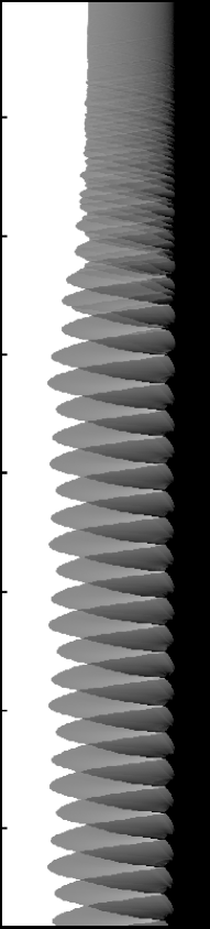
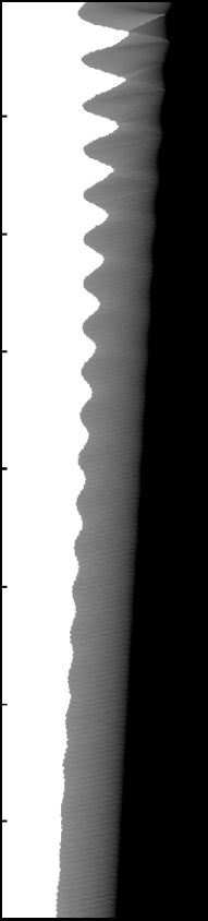
Figure 1: Spacetime diagrams of a radiative shock for $M=10$, $\alpha=0.0$ (cf. Fig. 3 in Strickland & Blondin SB1995 (1995)). The tick marks on the vertical axis are in units of $25L_{\rm c}/v_{0}$ where $L_{\rm c}$ is the cooling length of the shock (see Strickland & Blondin SB1995 (1995)). The width of the horizontal axis is $1.88L_{\rm c}$. The supersonic flow enters the grid from the left, and the cooled postshock gas flows off the grid to the right. The grayscale shows the density of the gas, with lighter shades signifying diffuse gas and darker regions denoting higher density. In the left panel, $q_{0}=0$, and the system exhibits linear growth for the first $\sim 40\%$ of the run. In the right panel, where $q_{0}=150$, the initial conditions are far from equilibrium for a mass-loaded shock, and the system exhibits powerful oscillations, though these are quickly damped as expected from the linear stability analysis in Sec. 2.

To investigate the effect of mass-loading on the stability of a radiative shock, we have computed 1D numerical calculations for a Mach 10 shock with the condition that $\alpha=0.0$. Our computations were initialized in a similar fashion to that presented by Strickland & Blondin (SB1995 (1995)) for the case of an isolated planar shock, and were performed using the same hydrodynamical code, VH-1 (see Blondin et al. BKFT1990 (1990)).

Briefly, we assumed a steady-state radiative shock in the centre of the grid, with pre-shock flow from the left grid boundary, and cold, dense, post-shock material exiting the right grid boundary. The most common downstream condition for similar calculations in the literature is that of a reflecting wall, but a continuous outflow has several benefits. For instance, feedback between the cold dense post-shock layer and the cooling gas is properly treated, and the problem more closely resembles the common occurence of an isolated shock in the interstellar medium. We also repeat the cautionary note of Strickland & Blondin (SB1995 (1995)) that the boundary conditions play an important role in determining the stability of the shock. Therefore, it is desirable to place the shock well away from grid boundaries. We refer the reader to Strickland & Blondin (SB1995 (1995)) for a fuller description of the code and initial conditions. In our runs we assumed $\gamma=5/3$.

In the left panel of Fig. 1 we show the development of the overstability for a Mach 10 flow with $\alpha=0.0$ and $q_{0}=0.0$ (i.e. no mass-loading). The pre-shock density and velocity are set to unity. At the beginning of the simulation, corresponding to the top of the plot, the flow is initialized as closely as possible to the steady state solution for a radiative shock with no mass-loading. The overstability is excited from weak perturbations produced by the numerical mapping of the steady state solution onto the computational grid. Linear growth was observed for about the first 40% of the run, after which the amplitude of the oscillations saturate and the system enters the nonlinear regime. The behaviour shown in the left panel of Fig. 1 is in excellent agreement with Fig. 3 of Strickland & Blondin (SB1995 (1995)) where the overstability for a Mach 40 flow is displayed.

In the right panel of Fig. 1 we show the evolution of a mass-loaded radiative shock with $q_{0}=150.0$ and $\lambda=5/2$. The process of mass-loading increases the density and thermal pressure, and decreases the temperature and velocity of the flow. The pressure increase causes the shock position to initially expand away from the dense cooling layer. However, the enhanced density leads to more rapid cooling, and thermal pressure support is soon lost. This causes the shock to reverse its direction of motion and to fall towards the cold dense layer. The shocked gas is then repressurized and this cycle is repeated. With each cycle, the amplitude of the oscillations decreases as the mass-loading damps this instability.

With $\alpha=0.0$, $\mathcal{L}=1$, $\mu/{\rm R}=1$ and the post-shock values $\rho=4$, $T=0.193$, Eq. 19 shows that we require $q_{0}>13$ for mass-loading to begin to damp the overstability. In practice, we find that we need values appreciably larger than this for strong damping, although the oscillation amplitude does decrease slightly for values of $q_{0}$ near 13. There are a couple of reasons why we need higher values of $q_{0}$ than suggested by Eq. 19. The principal reason is due to the fact that adding mass to the shocked gas decreases the cooling timescale while simultaneously increasing the mass-loading timescale. Hence, while the initial addition of mass to the immediate post-shock flow may be at a rate such that the mass-loading timescale is less than the cooling timescale, the difference between the two timescales will diminish with time and may even be reversed.

Secondly, the large dynamic range in temperature which exists for high Mach number shocks (e.g., for a Mach number of 40, the immediate post-shock temperature is almost 3 orders of magnitude greater than the ambient temperature) leads to a smaller value of $T_{\rm avg}/T_{\rm ps}$ than is the case for lower Mach number shocks. Here $T_{\rm avg}$ is the average temperature over the cooling length of the shock, and $T_{\rm ps}$ is the immediate post-shock temperature. We find that as we reduce the shock Mach number, the value of $q_{0}$ needed for significant damping more closely matches that from Eq. 19.

While we have not been concerned with the ionization state of the gas in this model, it is worth noting that the radiative cooling rate can be greatly enhanced when neutral gas is introduced into hot plasma, and that the ionization energy can also be significant under such conditions (Slavin et al. SSB1993 (1993)).

4 Discussion

As a relevant example, the above results can be applied to planetary nebulae (PNe). Such objects often display clumps which appear to mass-load the shocked wind of the central star. The clumps were presumably formed by instabilities in the atmospheres of the red supergiant stars, prior to the evolution of the central star into a hot object with a fast wind. In the following we derive relationships for the number density of clouds and their total mass, with the condition that mass injection from the clouds is able to suppress the thermal instability.

Since the central stars of PNe appear to fall into 3 groups (e.g., Kudritzki et al. K1997 (1997)), with winds spanning a large range of mass-loss rate ($\hbox{${\dot{M}}$}\,\sim 10^{-9}-10^{-6}\hbox{${\rm\hbox{${\rm\thinspace M_{\odot}}$}{\rm\thinspace yr}^{-1}\,}$}$), we choose not to focus on an individual nebula. Instead, we note that the typical thermal pressure in PNe, wind-blown-bubbles, and starburst superwinds is comparable to the pressure in clumps embedded within them, $P/k\sim 10^{7}\;{\rm cm^{-3}\;K}$. In PNe, this must balance the ram pressure from the wind of the central star. The post-shock number density is then $n=4\times 10^{-7}v_{7}^{-2}k/\mu(P/k)_{7}=55v_{7}^{-2}(P/k)_{7}\;\hbox{${\rm{\rm\thinspace cm}^{-3}\,}$}$, where $v_{7}$ is the wind speed in units of $1000\hbox{${\rm{\rm\thinspace km}{\rm\thinspace s}^{-1}\,}$}$ and $(P/k)_{7}$ is $P/k$ in units of $10^{7}\;{\rm cm^{-3}\;K}$. In the last step, and throughout the remainder of these calculations, we set $\mu=10^{-24}\;{\rm g}$. The post-shock temperature, $T=1.36\times 10^{5}v_{7}^{2}\;{\rm K}$.

To suppress the thermal instability by mass-loading, Eq. 19 gives $q_{0}\mathrel{\hbox to0.0pt{\lower 3.0pt\hbox{$\sim$}\hss}\raise 2.0pt\hbox{$>$}}10^{-32}v_{7}^{-7}(P/k)_{7}^{2}\;\hbox{${\rm{\rm\thinspace g}{\rm\thinspace cm}^{-3}{\rm\thinspace s}^{-1}\,}$}$, where we have adopted $\Lambda=1.33\times 10^{-19}/\mu^{2}$ and $\alpha=-{1\over 2}$ (cf. Kahn K1976 (1976)), and substituted for $T$ and $n$. The mass evaporation rate from a single clump is $\dot{m}=2.75\times 10^{4}T^{5/2}R_{\rm pc}(30/{\rm ln}\Lambda)\;\hbox{${\rm{\rm\thinspace g}{\rm\thinspace s}^{-1}\,}$}$ (Cowie & McKee CM1977 (1977)), where $T$ is the temperature of the ambient surroundings, and $R_{\rm pc}$ is the radius of the clump in parsecs. Since ${\rm ln}\Lambda\sim 30$, $\dot{m}\sim 1.9\times 10^{17}v_{7}^{5}R_{\rm pc}\;\hbox{${\rm{\rm\thinspace g}{\rm\thinspace s}^{-1}\,}$}$, and the required number density of clumps is $n_{\rm c}=q_{0}/\dot{m}\mathrel{\hbox to0.0pt{\lower 3.0pt\hbox{$\sim$}\hss}\raise 2.0pt\hbox{$>$}}1.6\times 10^{6}v_{7}^{-12}R_{\rm pc}^{-1}(P/k)_{7}^{2}\;{\rm pc^{-3}}$.

Observations of the Helix nebula (NGC 7293) indicate that the density within the clumps, $N_{\rm c}\sim 10^{6}\hbox{${\rm{\rm\thinspace cm}^{-3}\,}$}$, while they are unresolved on spatial scales of $\sim 10^{-3}{\rm\thinspace pc}$ (O’Dell & Handron DH1996 (1996)). Adopting $R_{\rm pc}=10^{-3}$, $v_{7}=2$, and $(P/k)_{7}=1$ yields a number density of clumps of $n_{\rm c}\mathrel{\hbox to0.0pt{\lower 3.0pt\hbox{$\sim$}\hss}\raise 2.0pt\hbox{$>$}}4\times 10^{5}\;{\rm pc^{-3}}$. Since the radius of the Helix nebula is $\sim 0.2\;{\rm\thinspace pc}$, we then expect $\sim 1600$ clumps, with a total mass of $\sim 0.1\;\hbox{${\rm\thinspace M_{\odot}}$}$. While these estimates are in good agreement with observational inferences from the Helix nebula, small changes in $v_{7}$ can greatly affect these values. For the evaporation to be smooth on a spatial scale of $1/k_{\rm m}$, we require that the clumps are smaller than $L=2\pi/k_{\rm m}$, i.e. $L\mathrel{\hbox to0.0pt{\lower 3.0pt\hbox{$\sim$}\hss}\raise 2.0pt\hbox{$<$}}1.5\times 10^{-2}v_{7}^{6}(P/k)_{7}^{-1}{\rm\thinspace pc}$. With the above parameters, $L\mathrel{\hbox to0.0pt{\lower 3.0pt\hbox{$\sim$}\hss}\raise 2.0pt\hbox{$<$}}1{\rm\thinspace pc}$, and is consistent with the derived number density of clumps.

- (1) Blondin, J.M., Cioffi, D.F., 1989, ApJ, 345, 853
- (2) Blondin, J.M., Kallman, T.R., Fryxell, B.A., Taam, R.E., 1990, ApJ, 356, 591
- (3) Chevalier, R.A., Imamura, J.N., 1982, ApJ, 261, 543
- (4) Cowie, L.L., McKee, C.F., 1977, ApJ, 211, 135
- (5) Falle, S.A.E.G., 1975, MNRAS, 172, 55
- (6) Falle, S.A.E.G., 1981, MNRAS, 195, 1011
- (7) Field, G.B., 1965, ApJ, 142, 531
- (8) Gaetz, T.J., Edgar, R.J., Chevalier, R.A., 1988, ApJ, 329, 927
- (9) Imamura, J.N., Wolff, M.T., Durisen, R.H., 1984, ApJ, 276, 667
- (10) Kahn, F.D. 1976, A&A, 50, 145
- (11) Kudritzki, R.P., Mendez, R.H., Puls, J., McCarthy, J.K., 1997, in IAU Symp. 180, Planetary Nebulae, eds. H.J. Habing and H.J.G.L.M. Lamers (Dordrecht: Kluwer), 64
- (12) Langer, S., Chanmugam, G., Shaviv, G., 1981, ApJ, 245, L23
- (13) McKee, C.F., Cowie, L.L., 1977, ApJ, 215, 213
- (14) O’Dell, C.R., Handron, K.D., 1996, AJ, 111, 1630
- (15) Pittard, J.M., Dyson, J.E., Hartquist, T.W., 2001, A&A, 367, 1000
- (16) Slavin, J.D., Shull, J.M., Begelman, M.C., 1993, ApJ, 407, 83
- (17) Strickland, R., Blondin, J.M., 1995, ApJ, 449, 727
- (18) Walder, R., Folini, D., 1996, A&A, 315, 265