Magnetorotationally-Driven Galactic Turbulence and
the Formation of Giant Molecular Clouds

Abstract

Giant molecular clouds (GMCs), where most stars form, may originate from self-gravitating instabilities in the interstellar medium. Using local three-dimensional magnetohydrodynamic simulations, we investigate ways in which galactic turbulence associated with the magnetorotational instability (MRI) may influence the formation and properties of these massive, self-gravitating clouds. Our disk models are vertically stratified with both gaseous and stellar gravity, and subject to uniform shear corresponding to a flat rotation curve. Initial magnetic fields are assumed to be weak and purely vertical. For simplicity, we adopt an isothermal equation of state with sound speed $c_{\rm s}=7\,{\rm km\,s^{-1}}$. We find that MRI-driven turbulence develops rapidly, with the saturated-state Shakura & Sunyaev parameter $\alpha\sim(0.15-0.3)$ dominated by Maxwell stresses. Many of the dimensionless characteristics of the turbulence (e.g. the ratio of the Maxwell to Reynolds stresses) are similar to results from previous MRI studies of accretion disks, hence insensitive to the degree of vertical disk compression, shear rate, and the presence of self-gravity – although self-gravity enhances fluctuation amplitudes slightly. The density-weighted velocity dispersions in non- or weakly self-gravitating disks are $\sigma_{x}\sim\sigma_{y}\sim(0.4-0.6)c_{\rm s}$ and $\sigma_{z}\sim(0.2-0.3)c_{\rm s}$, suggesting that MRI can contribute significantly to the observed level of galactic turbulence. The saturated-state magnetic field strength $\bar{B}\sim 2\mu$G is similar to typical galactic values. When self-gravity is strong enough, MRI-driven high-amplitude density perturbations are swing-amplified to form Jeans-mass ($\sim 10^{7}{\rm\,M_{\odot}}$) bound clouds. Compared to previous unmagnetized or strongly-magnetized disk models, the threshold for nonlinear instability in the present models occurs for surface densities at least 50% lower, corresponding to the Toomre parameter $Q_{\rm th}\sim 1.6$. We present evidence that self-gravitating clouds like GMCs formed under conditions similar to our models can lose much of their original spin angular momenta by magnetic braking, preferentially via fields threading near-perpendicularly to their spin axes. Finally, we discuss the present results within the larger theoretical and observational context, outlining directions for future study.

1 Introduction

It has long been a challenge to understand the origins of giant molecular clouds (GMCs). Observations and theory both favor “top-down” (instability) rather than “bottom-up” (coagulation) mechanisms, at least for the most massive clouds ($\sim 10^{5}-10^{6}{\rm\,M_{\odot}}$) in which the majority of the molecular material is found and the preponderance of stars are born (e.g., Blitz 1993). The principal difficulty with stochastic coagulation is that it proceeds much too slowly to achieve GMC masses given other constraints (e.g., Blitz & Shu 1980); recent support for this view includes the observed lack of raw material in small clouds within spiral arms (Heyer & Terebey, 1998), and the conclusion from numerical simulations that magnetohydrodynamic (MHD) turbulence cannot prevent gravitational collapse within clouds that exceed the magnetic critical mass (e.g., Ostriker, Stone, & Gammie 2001; Heitsch, Mac Low, & Klessen 2001). The latter result implies that intermediate products of coagulation $\lower 2.15277pt\hbox{$\;\buildrel>\over{\sim}\;$}10^{4}{\rm\,M_{\odot}}$, if they were created, would undergo rapid star formation and be destroyed by the associated energy feedback before subsequent mergers could attain $\sim 10^{6}{\rm\,M_{\odot}}$.

The two main classes of instabilities proposed for GMC formation are Parker and self-gravitating modes, and their hybrids (e.g., Elmegreen 1995). Although the azimuthal wavelengths and initial growth rates of Parker modes suggest they could prompt cloud formation in spiral arms (e.g., Mouschovias, Shu, & Woodward 1974), numerical simulations have recently shown that nonlinear development favors short radial wavelengths and saturates at moderate amplitudes. The low-density-contrast structures that develop do not appear to be the primary progenitors of gravitationally-bound GMCs (J.Kim et al., 2000, 2001; Kim, Ostriker, & Stone, 2002, hereafter Paper III).

Direct self-gravitating instabilities have similar preferred azimuthal scales and growth rates to Parker modes, but are not self-limiting in the nonlinear regime. In regions without spiral structure, epicyclic motion can temporarily conspire with shear in the swing amplifier process (Toomre, 1981) to yield gravitational runaway provided a sufficient surface density. Based on two-dimensional simulations, Kim & Ostriker (2001, hereafter Paper I) found a nonlinear instability threshold at Toomre $Q_{\rm th}=1.2-1.4$ (for definition, see eq. [4] below) for a range of magnetic field strengths; from three-dimensional simulations with zero or thermal-equipartition magnetic fields, Paper III found $Q_{\rm th}\lower 2.15277pt\hbox{$\;\buildrel<\over{\sim}\;$}1$.

In high-density portions of spiral arms, local reduction or reversal of shear suppresses swing amplification, but magneto-Jeans instability (see Lynden-Bell 1966; Elmegreen 1987 and Paper I) can yield self-gravitating growth since magnetic torques between azimuthally-adjacent regions limit the epicyclic motion and spin-up of contracting condensations. Numerical simulations in thin-disk models (Kim & Ostriker, 2002, hereafter Paper II) have shown that the magneto-Jeans instability in spiral arms first leads to growth of gaseous spurs, which then fragment into Jeans-scale condensations.

The investigations of cloud formation in Papers I-III considered either two-dimensional or three-dimensional models with zero or strong magnetic fields (to study Parker modes). Under more realistic galactic conditions with subthermal mean magnetic fields, however, new dynamical effects are introduced by the action of the magnetorotational instability (MRI). Although the MRI has primarily been studied in the context of accretion disks, Sellwood and Balbus (1999) proposed that MRI and related processes may be important for maintaining turbulence in the outer H I disks of galaxies where the star formation rate (and supernova rate) is low. The recent calculations of Wolfire et al. (2003) showing that a cold phase must be present in the far outer Milky Way support the notion that MRI-driven turbulence prevents the settling and gravitational fragmentation of a thin, cold gas layer that would otherwise ensue.

To understand why the MRI is likely to be important in galaxies, it is helpful to consider the instantaneous instability criterion for MRI modes $\propto e^{i{\bf k\cdot x}}$,

$${({\bf k\cdot}{\bf v}_{\rm A})^{2}\over\Omega^{2}}{|{\bf k}|^{2}\over k_{z}^{2}}<-2{d\ln\Omega\over d\ln R}\equiv 2q$$ (1)

(e.g., Balbus & Hawley 1998). Here, $\Omega(R)$ is the disk’s angular rotation profile, and ${\bf v}_{\rm A}\equiv{\bf B}/(4\pi\rho)^{1/2}$ in terms of the local density $\rho$ and mean magnetic field $\bf B$. Physically, this criterion represents the need for (moderate) magnetic tension torques between radially-displaced fluid elements that are azimuthally sheared by the background flow to reinforce the initial perturbations in angular momentum (Balbus & Hawley, 1991). In a galaxy without strong spiral structure or in interarm regions when a prominent spiral pattern exists, $q\sim 1$ and unstable MRI modes with a variety of wavenumbers will be present.

The detailed dynamical characteristics and consequences of MRI-driven turbulence in galaxies have not previously been studied directly. Although the literature contains many theoretical and numerical treatments of MRI (e.g. Balbus & Hawley 1991; Hawley, Gammie, & Balbus 1995; Stone et al. 1996; Miller & Stone 2000; Hawley & Krolik 2002, see also Balbus & Hawley 1998; Stone et al. 2000 and references therein), these works have focused primarily on angular momentum transport in accretion disks around stars and black holes. These accretion disks differ significantly from galactic disks in that the latter are self-gravitating, have flat rotation curves rather than Keplerian rotation, and are more vertically compressed by both gaseous self-gravity and external stellar gravity rather than solely by a tidal stellar potential. How do the physical properties of a disk affect the level and characteristics of the saturated-state turbulence driven by MRI? How does this turbulence nonlinearly interact with self-gravity to form GMC-like structures in galactic disks? In this paper, we address these and related questions by performing and analyzing a suite of three-dimensional MHD simulations.

As in Paper III, our disk models are local, isothermal, and vertically stratified. Initial magnetic fields are assumed to have a weak, uniform strength, pointing in the vertical direction (but note that after MRI develops, $\bf B$ becomes toroidally-dominated). The background potential corresponds to that yielding a flat galactic rotation curve. In this first work on galactic MRI, we do not consider other features such as stellar spiral structure and effects of the multi-phase ISM that would be present in real galaxies; these effects will be considered in subsequent work.

In §2, we briefly describe our model parameters and computational methods. In §3.1, we investigate the characteristics of MRI-driven turbulence in our non- or weakly self-gravitating models, and compare with results from previous accretion disk simulations. We directly measure the density-weighted velocity dispersions to assess whether MRI can be a significant source of turbulence in the diffuse ISM. We also discuss the role played by self-gravity in supplying turbulent energy to the ISM. In §3.2, we present results on $Q$ thresholds for the formation of gravitationally bound clouds in MRI-unstable disks, with comparison to our model results from Paper III. The properties of the bound clouds formed and the role of magnetic fields in braking their rotational spins is briefly discussed as well. Finally, in §4 we conclude and discuss our findings and related issues within a larger context, noting outstanding questions related to galactic turbulence and GMC formation that will be the focus of future work.

2 Methods and Model Parameters

For local, three-dimensional simulations of vertically stratified, MRI-unstable, galactic gas disks, we use the same numerical code and model formulation described in Paper III, with the exception that we modify the strength and spatial distribution of the initial magnetic field. We adopt an isothermal condition in both space and time, with an effective isothermal speed of sound $c_{\rm s}=7{\,\rm\,km\,s^{-1}}$, and solve for an initial vertical density distribution $\rho_{0}(z)$ in hydrostatic equilibrium between the thermal pressure gradient and the total (gaseous plus stellar) gravity. For the strength of external stellar gravity, we define

$$s_{0}\equiv\left(\frac{\sigma_{*,z}\Sigma_{0}}{c_{\rm s}\Sigma_{*}}\right)^{2},$$ (2)

where $\sigma_{*,z}$ and $\Sigma_{*}$ are the vertical velocity dispersion and surface density of stars, respectively, while $\Sigma_{0}$ denotes the gas surface density (see Paper III). To represent average disk conditions, we take $s_{0}=1$ corresponding to $\sigma_{*,z}\approx 20{\,\rm\,km\,s^{-1}}$, $\Sigma_{*}\approx 35\,{\rm\,M_{\odot}}\,{\rm\,pc}^{-2}$, and $\Sigma_{0}\approx 13\,{\rm\,M_{\odot}}\,{\rm\,pc}^{-2}$ (e.g., Kuijken & Gilmore 1989; Holmberg & Flynn 2000). Note that these values give comparable stellar-disk and gas-disk vertical gravity at $|z|\sim H$, where $H$ stands for the gas disk scale height (Paper III).

We introduce an initial uniform magnetic field, $\mathbf{B}_{0}=B_{0}\mathbf{\hat{z}}$, that points in the vertical ($\mathbf{\hat{z}}$) direction. We parameterize its strength using

$$\beta(z)\equiv\frac{c_{\rm s}^{2}}{v_{\rm A}^{2}}=\frac{4\pi\rho_{0}(z)c_{\rm s}^{2}}{B_{0}^{2}},$$ (3)

where $v_{\rm A}\equiv B_{0}/(4\pi\rho_{0})^{1/2}$ is the Alfvén speed. In the numerical models presented in this paper, we adopt $\beta(0)=100$ or 400. The physical value of the initial midplane magnetic field is thus $\sim 0.2-0.4\mu$G. Since the density drops off with height, high-latitude regions may have $\beta(z)<1$ with which the growth of MRI is ineffective, but the weak midplane magnetic fields guarantee that the most unstable wavelength of MRI is confined within $|z|\lower 2.15277pt\hbox{$\;\buildrel<\over{\sim}\;$}H$. Note that although the initial magnetic field in our models is primarily vertical (a numerical expedient that yields rapid growth of MRI), this condition is not inconsistent with observations of preferentially azimuthal galactic $\bf B$-fields, because the saturated-state MRI has mainly toroidal $\bf B$, as we shall show in §3.1. Also note that the amplitudes of saturated-state turbulence depend on the net flux for pure-$z$ initial $B$-fields (Hawley, Gammie, & Balbus, 1995, hereafter HGB); we will briefly discuss this in §3.1.1 and §4.1. Other classes of initial magnetic field distributions that have been studied in non-self-gravitating MRI simulations (e.g., HGB; Stone et al. 1996; Miller & Stone 2000) contain zero net magnetic flux. Since simulations which begin with zero net flux take much longer to reach saturated turbulence, we have focused on uniform vertical field models in this paper. Further exploration of intermediate field strength and/or orientation may yield interesting results; we shall, however, defer broader parameter surveys to future investigations.

An important measure of susceptibility to gravitational instability is the Toomre $Q$ parameter (Toomre, 1964)

$$Q\equiv\frac{\kappa c_{\rm s}}{\pi G\Sigma_{0}}=1.4\left(\frac{c_{\rm s}}{7.0{\rm\,km\,s^{-1}}}\right)\left(\frac{\kappa}{36\,{\rm km\,s^{-1}\,kpc^{-1}}}\right)\left(\frac{\Sigma_{0}}{13\,{\rm\,M_{\odot}}{\rm\,pc}^{-2}}\right)^{-1},$$ (4)

where $\kappa$ is the epicyclic frequency. We evolve models with $Q$ in the range of 1 to 2 to represent various conditions in disk galaxies (e.g., Martin & Kennicutt 2001). Note that the often-cited critical value of $Q_{\rm th}=1$ applies to axisymmetric instability in an infinitesimally thin disk. Even in unmagnetized cases, finite disk thickness generally reduces the critical $Q$ value for axisymmetric instability to $Q_{\rm th}=0.676$ for purely self-gravitating disk with $s_{0}=\infty$ (Goldreich & Lynden-Bell, 1965a; Gammie, 2001) and $Q_{\rm th}=0.75$ for a disk with $s_{0}=1$ (Paper III). Therefore, our model disks having $Q\lower 2.15277pt\hbox{$\;\buildrel>\over{\sim}\;$}1$ and $s_{0}=1$ are all stable to axisymmetric perturbations.

We integrate the time-dependent, compressible, ideal MHD equations in a local Cartesian reference frame whose center orbits the galaxy with a fixed angular velocity $\Omega=\Omega(R_{0})$ at a galactocentric radius $R_{0}$. In this local frame, the equilibrium velocity due to galactic differential rotation relative to the center of the box is given by $\mathbf{v_{0}}=-q\Omega x\mathbf{\hat{y}}$, where $q\equiv-d\ln\Omega/d\ln R|_{R_{0}}$ is the local shear rate and $x\equiv R-R_{0}$ and $y\equiv R_{0}(\phi-\Omega t)$ refer to radial and (rotating-frame) azimuthal coordinates, respectively. We adopt $q=1$, corresponding to a flat rotation curve. The basic equations we solve are presented in Paper III. We use a modified version of the ZEUS code (Stone & Norman, 1992a, b) with a hybrid Green function/FFT solver for the Poisson equation (Paper III) and applying a velocity decomposition method (Paper I) for less diffusive transport of hydrodynamic variables under strong shear conditions. For improved numerical performance in the low-density “coronal” region, we employ the Alfvén limiter algorithm of Miller & Stone (2000) with the limiting speed of the displacement current, $c_{\rm lim}=8c_{\rm s}$. We adopt periodic boundary conditions in the $y$- and $z$-directions and shearing-periodic conditions at the $x$-boundaries (HGB). From test runs with an inflow/outflow $z$-boundary, we have confirmed that evolution of the midplane portions of the disk is quite insensitive to the imposed vertical boundary conditions.

The $(x,y,z)$ dimensions of our computational box are $(L_{x},L_{y},L_{z})=(25,25,6)\times H$. Since an unmagnetized disk with $s_{0}=1$ has $H\approx 160$ pc for the solar neighborhood value $\Omega=26{\,\rm km\,s^{-1}\,kpc^{-1}}$ (Paper III), the total mass contained in the simulation domain is $M_{\rm tot}=2.1\times 10^{8}{\rm\,M_{\odot}}(\Sigma_{0}/13{\rm\,M_{\odot}}{\rm\,pc}^{-2})(H/160\;{\rm pc})^{2}$, which is about 20 times larger than the two-dimensional Jeans mass,

$$M_{\rm J,2D}\equiv\frac{c_{\rm s}^{4}}{G^{2}\Sigma_{0}}=10^{7}{\rm\,M_{\odot}}\left(\frac{c_{\rm s}}{7\,{\rm km\,s^{-1}}}\right)^{4}\left(\frac{\Sigma_{0}}{13{\rm\,M_{\odot}}{\rm\,pc}^{-2}}\right)^{-1}.$$ (5)

The numerical resolution is $128^{3}$ zones for all models. We apply initial perturbations only to the velocity using spatially uncorrelated, random fluctuations multiplied by the background density profile $\rho_{0}(z)$. The amplitude of the perturbations is determined such that Max($|\delta\mathbf{v}|/c_{\rm s})=0.25$ at the disk midplane. We will use the orbital period $t_{\rm orb}\equiv 2\pi/\Omega=2.4\times 10^{8}\,{\rm yrs}\,(\Omega/26\,{\rm km\,s^{-1}\,kpc^{-1}})^{-1}$ as the time unit in our presentation.

3 Simulations and Results

To investigate MRI-driven turbulence and its interaction with self-gravity, we have performed 7 numerical simulations. The important parameters and the simulation outcomes for each model are listed in Table 1. Column (1) gives the label for each run. Columns (2) and (3) are the Toomre $Q$ parameter and the initial field strength in terms of the plasma parameter at the disk midplane $\beta(0)$ (see eqs. [3] and [4]). Column (4) indicates whether self-gravity is included in the dynamical evolution. Note that self-gravity in the models with “yes” is slowly turned on only after turbulence becomes saturated, starting at $t/t_{\rm orb}=4.1$. Note also that “no” self-gravity models still include the initial total gravity that maintains the unperturbed equilibrium density profile. Column (5) gives the final simulation outcome: “unstable” indicates the formation of gravitationally bound condensations, while “stable” indicates fluctuating density fields without any condensations.

Columns (6) and (7) summarize the scaling relations among the time and space averaged stresses and magnetic energy density in the stable models: $R_{xy}\equiv\langle\langle\rho v_{x}\delta v_{y}\rangle\rangle$ and $M_{xy}\equiv\langle\langle-B_{x}B_{y}/4\pi\rangle\rangle$ are the Reynolds and Maxwell stresses, respectively; $T_{xy}=R_{xy}+M_{xy}$ is the total stress; $E_{B}\equiv\langle\langle B^{2}/8\pi\rangle\rangle$ is the total magnetic energy density. Here, the double bracket $\langle\langle\,\rangle\rangle$ denotes a time- and space-average. Finally, columns (8)-(10) give the time-averaged values of density-weighted velocity dispersions $\langle\rho\delta v_{i}^{2}\rangle^{1/2}/\langle\rho\rangle^{1/2}$ for the stable models, where the single bracket $\langle\,\rangle$ denotes a space average (with the subscript $i=x$, $y$, or $z$). For columns (6)-(10), time averages are taken typically over 2 orbits after MRI saturation.

3.1 Non-Collapsing Models

In this subsection we describe the evolution of non-self-gravitating and weakly self-gravitating models that do not form bound condensations. Of previous work, nonstratified simulations of HGB with vertical initial magnetic fields, or stratified disks of Stone et al. (1996, hereafter SHGB) with sinusoidally varying fields, are similar to our models. Both HGB and SHGB differ from the present models in that they used a Keplerian rotation profile appropriate to accretion disks. We shall compare the results of our simulations with those of HGB and SHGB.

3.1.1 MRI-Driven Turbulence

We begin with non-self-gravitating model A. Figure 1 plots evolutionary histories of the maximum density ($\rho_{\rm max}$, solid lines) and density dispersion ($\langle\delta\rho^{2}\rangle^{1/2}$, dotted lines) of model A together with those of the other models. Snapshots of the perturbed density at four time epochs of model A are shown in Figure 2.

The initial equilibrium of model A is a vertically stratified, shearing disk with $q=1$ and threaded by uniform $B_{z}$ with $\beta(0)=100$. During the initial relaxation stage ($t/t_{\rm orb}\lower 2.15277pt\hbox{$\;\buildrel<\over{\sim}\;$}2$), small-scale modes have low-amplitude (a few percent) density fluctuations, as shown in the perturbed density plot (Fig. 1$a$). As the system finds the most unstable MRI mode, however, density fluctuations begin to grow rapidly. The dominance of the most-unstable axisymmetric mode (Balbus & Hawley, 1991) is evident in the character of the density fluctuations of Fig. 2a,b, which are correlated with the “channel flow” in the velocity field (Hawley & Balbus 1991; see below). Linear theory predicts that for the parameters in model A, the maximum growth rate of the MRI in model A is $\gamma_{\rm max}=\Omega/2$, which occurs for vertical wavelength

$$\lambda_{\rm max}\approx 200\;{\rm pc}\;\left(\beta(0)\over 100\right)^{-1/2}\left(c_{\rm s}\over 7\,{\rm km\,s^{-1}}\right)\left(\Omega\over 26\,{\rm km\,s^{-1}\,kpc^{-1}}\right)^{-1}$$ (6)

(e.g., Balbus & Hawley 1998). Since $\lambda_{\rm max}$ fits well within a density scale height of the disk (i.e., $\lambda_{\rm max}/2<H$), the MRI in model A develops similarly to the way it would in a uniform medium. The predicted maximum growth rate, $\gamma_{\rm max}$, marked by the dashed line in Figure 1$a$, is indeed in good agreement with the simulation results.

Because the fastest growing mode in model A approximates an exact nonlinear solution of the full MHD equations in the incompressible limit (Goodman & Xu, 1994), it can grow to very large amplitude while preserving its essential character. As the mode grows, the whole flow in model A becomes dominated by this “channel solution,” in which fluid elements in alternating horizontal layers that have larger (smaller) azimuthal velocity than the background tends to move radially outward (inward). This inward/outward flow drags the magnetic fields radially in directionally alternating layers, and the sheared azimuthal motion produces corresponding alternating layers of toroidal magnetic field. As the amplitude of $v_{A,\varphi}$ becomes large, vertical magnetic pressure gradients compress the disk in alternating layers. The gas associated with the over-dense regions at $|z|<0.08L_{z}$ in Figure 2$b$ is streaming radially inward, while the layers surrounding it are moving outward. After the channel mode grows to very large amplitude, the nonaxisymmetric parasitic instability (Goodman & Xu, 1994) develops to break up the flow into smaller-scale turbulence (Fig. 2c,d). Direct growth of nonaxisymmetric MRI may also contribute to small scale kinetic and magnetic turbulence (HGB). At $t/t_{\rm orb}\lower 2.15277pt\hbox{$\;\buildrel>\over{\sim}\;$}4$, the turbulence has achieved a saturated state with large fluctuation amplitudes in all physical variables.

The evolution of averaged disk properties due to the MRI is illustrated in Figure 3, where we plot horizontally-averaged densities, plasma $\beta$, magnetic and perturbed kinetic energy densities, and Maxwell and Reynolds stresses of model A at times $t/t_{orb}=0,3,4,5$. We also list in Table 2 the volume and time averages of various physical quantities averaged over $t/t_{\rm orb}=4-6$. Magnetic fields are amplified to attain levels $\beta\sim 1-10$ at MRI saturation (Fig. 3$b$). The regions above $|z|=2H$ have $\beta<0.5$, consistent with the results of SHGB and Miller & Stone (2000) that MRI in a stratified disk produces a moderately-magnetized disk midplane surrounded by a magnetically-dominated corona. Overall, the magnetic energy density is dominated by the azimuthal component ($B_{y}^{2}/8\pi$), and is larger than the perturbed kinetic energy density by a factor of 2 to 7, with the largest value at late times occurring about a scale height above the midplane (Fig. 3$c$). Although the kinetic energy density is not more than $\sim 10\%$ of the central thermal pressure and the velocity fluctuations are subsonic at the midplane, the magnetic fields are strong enough to drive supersonic motions in the low-density, high-altitude regions.

Tables 1 and 2 suggest that in terms of Shakura & Sunyaev (1973) $\alpha$ parameter describing the radial transport of angular momentum, the total dimensionless stress is $\alpha\equiv T_{xy}/P_{0}(0)\approx 0.16$, with the Reynolds stress contributing only $\sim 10\%$ of the total (see also Fig. 3$d$). This demonstrates that magnetic fields bear primary responsibility for mediating mass accretion in an MRI-unstable disk (Balbus & Hawley, 1998). During the entire linear and nonlinear evolution, the averaged density profile in $z$ is within $20\%$ of the initial distribution, although the amplified magnetic field thickens the disk slightly via its magnetic pressure support (Fig. 3$a$).

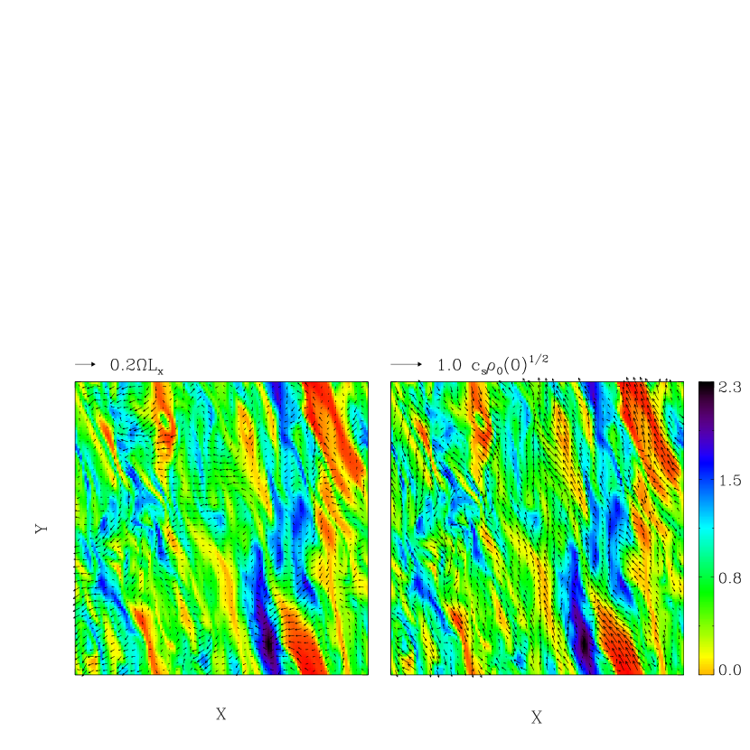
Figure 4: (left) Horizontal velocity and (right) magnetic field vectors at the midplane of model A at $t/t_{\rm orb}=5.6$ are overlaid on the maps of midplane density (greyscale; units $\rho_{0}(0)$).

In spite of the kinematic effect of the background shear, the density and magnetic fields are dominated by structure at relatively large spatial scales. Figure 4 displays the $x$-$y$ density structure as well as horizontal velocity and magnetic field vectors at the midplane of model A at $t/t_{\rm orb}=5.6$. Fourier power spectra of the density and the azimuthal component of the magnetic field averaged over $t/t_{\rm orb}=5-6$ in model A are plotted in Figure 5. Although the volume-averaged values of $B_{x}$ and $B_{y}$ are negligibly small (see Table 2), a constant-$z$ plane consists of a few magnetic domains in which $B_{x}$ and $B_{y}$ are distributed coherently; across the domains, the horizontal magnetic field reverses direction. For example, the right panel of Figure 4 shows that the midplane is dominated by negative-$B_{x}$ and positive-$B_{y}$: the midplane mean values of $B_{x}$ and $B_{y}$ are $-0.18$ and $0.38$ times $(4\pi P(0))^{1/2}$ at $t/t_{\rm orb}=5.6$, respectively. Given these large mean values of $\langle B_{x}\rangle$ and $\langle B_{y}\rangle$ in any layer at constant $z$, the magnetic field has to bend and reverse in the vertical direction in order to yield the small net volume averages of Table 2 (first three rows, second column). This field geometry is indeed consistent with Figure 5$b$, which shows that the maximum power of $B_{y}$ is attained in the $n_{x}=0=n_{y}$, $n_{z}=1$ mode; the $n_{y}=0$, $n_{x}=1=n_{z}$ mode is also strong. Here, integers $n_{x}\equiv k_{x}/2\pi L_{x}$, $n_{y}\equiv k_{y}/2\pi L_{y}$, and $n_{z}\equiv k_{z}/2\pi L_{z}$ denote the wavenumber in each direction. The dominant mode for $B_{y}$ at late times is thus still that associated with channel flow. The $B_{y}$ mode with next most power is coherent in the $y$ (azimuthal) direction and has a single reversal in the $z$ and $x$ (radial) directions.

Despite the fact that our model disk has lower shear and is more tightly vertically compressed than the models considered by HGB and SHGB, the characteristics of turbulence observed in the power spectra are similar. Among the similarities are (1) most of power is contained in modes with scales comparable to or larger than the disk scale height, (2) the turbulence is highly anisotropic, as the different slopes of the power spectra along the different axes implies, and (3) at well-resolved scales, the logarithmic slopes of the power spectra are similar to the $-11/3$ Kolmogorov spectrum (see HGB; SHGB). The kinetic-to-magnetic scaling ratios in our models are also similar to those in HGB. For instance, for a nonstratified model (Z4) with uniform magnetic fields, HGB found $R_{xy}/M_{xy}\approx 0.19$ and $T_{xy}/E_{B}\approx 0.66$, which are very similar to $R_{xy}/M_{xy}\approx 0.13-0.14$ and $T_{xy}/E_{B}\approx 0.64-0.65$ in models A and B of this paper (see Table 1).

The level of the turbulent fluctuations is, of course, dependent on the field strength and geometry, and possibly on other disk parameters. Having uniform vertical magnetic fields, model A exhibits stronger growth of MRI than a zero-net-$B_{z}$ model (IZ1) of SHGB. Table 2 shows that model A experiences fluctuations in the density with $\langle\delta\rho^{2}\rangle^{1/2}/\langle\rho\rangle\approx 1.018$ and in the total pressure with $\langle\delta P_{\rm tot}^{2}\rangle^{1/2}/\langle P_{\rm tot}\rangle\approx 0.629$, which are about an order of magnitude larger than in model IZ1 of SHGB. Comparing to the uniform-$B_{z}$ model Z4 of HGB, however, model A shows smaller turbulent fluctuation amplitudes. This is because the density stratification of model A makes high-$z$ fields effectively stronger (in terms of $\beta$), resulting in local MRI wavelengths at high latitudes that are larger than the vertical size of box. As a consequence, the resulting $\alpha$ in model A (which averages over both high-stress and low-stress volumes) is about a half of $\alpha\approx 0.31$ in model Z4 of HGB.

In practice, the vertical magnetic field will always be correlated in sign on some largest radial scale, and the extent of this correlated region – as well as the magnitude of the vertical magnetic flux over this scale – will affect the amplitudes of saturated-state turbulence. Even over short evolutionary times compared to the galactic lifetime, our models show growth in the $n_{z}=0$, $n_{y}=0$, $n_{x}=4$ component of the $B_{z}$ power spectrum, corresponding to correlated vertical magnetic field over radial scales comparable to the thickness of the disk. Although realistic values for the correlation scale and magnitude of $B_{z}$ are not known at present, this evidence of “dynamo” activity helps to motivate our incorporation of vertical flux in the initial conditions. While there are not yet predictions from simulations of the level of vertical magnetic fields that would develop over long timescales, one may speculate that vertical field would build up to values similar to those we adopt, since for much weaker vertical fields the fastest-growing MRI modes are at very small scales, and for much stronger vertical fields the MRI is stabilized (see also §4).

Radio observers of external face-on galaxies report line widths of order $\sim 6-10\,{\rm km\,s^{-1}}$ in extended regions of H I disks where no active star formation takes place (Dickey et al., 1990; van Zee & Bryant, 1999). Sellwood and Balbus (1999) proposed that in the absence of stellar energy inputs, the MRI may be important in producing large-scale random motions in these extended H I disks. A direct way to assess this specific proposal, and more generally to investigate the role of the MRI in driving galactic turbulence, is to measure the turbulent velocity dispersions from numerical simulations. Although the current models are idealized in ways that may significantly affect the results, it is useful to quantify the turbulence level for future comparisons. As Table 1 lists, the density-weighted one-dimensional velocity dispersions in the non-self-gravitating model A are found to be $\sigma_{x}=0.45c_{\rm s}$, $\sigma_{y}=0.43c_{\rm s}$, and $\sigma_{z}=0.23c_{\rm s}$. In dimensional units, these correspond only to $\sim 1.6-3.2\,{\rm km\,s^{-1}}$, much smaller than the observed line widths cited above (which however are not purely turbulent – see §4.1). The velocity dispersions are smallest in the vertical direction, indicating that buoyancy does not appreciably enhance turbulence. Model Z4 of HGB reports $\sigma_{x}=\sigma_{y}=0.43c_{\rm s}$ and $\sigma_{z}=0.22c_{\rm s}$, so that the density stratification has little effect on the velocity dispersion.

Finally, we compare the evolution of our disk models with Miller & Stone (2000), who performed stratified disk models with $q=3/2$. In their simulation with a pure $B_{z}$ field, strong axisymmetric channel flows quickly emerge and rise buoyantly, disrupting the initial disk structure. The system becomes magnetically dominated everywhere at the end of the run. As Figure 3 shows, however, our model A keeps its initial disk structure fairly intact even when the disk is highly turbulent. High-density parts of the disk in model A have subthermal magnetic fields at saturation rather than becoming magnetically dominated. In part, these differences may be due to the differences between the circumstellar-disk tidal gravity law $g_{z}=-\Omega^{2}z$ and the stronger vertical gravity provided by the gaseous and stellar disks in a galaxy. Within a scale height of the midplane, the galactic gravity is a factor $\sim 2-4$ larger for the present models compared to $g_{z}=-\Omega^{2}z$. This compresses the disk more tightly in the vertical direction, making the buoyant rise associated with the channel solution less efficient. With an initial field strength having $\beta(0)=12.5$ and a shear parameter $q=3/2$, MRI-amplified channel-flow magnetic fields in Miller & Stone (2000) are also much stronger than those in the present models, contributing to the destruction of the initial disk structure.

3.1.2 Effect of Self-Gravity on Turbulence

We now turn to models F and G, which have self-gravity included in their dynamical evolution but have surface densities below the (nonlinear) gravitational instability threshold. Thus, self-gravity in models F and G, with $Q=1.7$ and $2.0$, respectively, is not strong enough to engender formation of bound condensations, although it certainly enhances the fluctuation amplitudes of physical variables. Table 3 lists the volume and time averaged quantities (over $t/t_{\rm orb}=5.0-6.5$) in model F. The fluctuations in the perturbed density and total pressure, with $\langle\delta\rho^{2}\rangle^{1/2}/\langle\rho\rangle\approx 1.021$ and $\langle\delta P_{\rm tot}^{2}\rangle^{1/2}/\langle P_{\rm tot}\rangle\approx 0.646$, are quite similar in amplitudes to those in model A, but magnetic and perturbed kinetic energy densities in model F are increased by about 60%. Note, however, that the ratios $R_{xy}/M_{xy}$ and $T_{xy}/E_{B}$ are almost independent of the presence of self-gravity (Table 1), indicating that self-gravity, as well as the disk compression and shear parameter, does not change the angular-momentum-transport characteristics of MRI-driven turbulence significantly.

To gain some idea on the origin of the extra turbulent energy in the (weakly) self-gravitating model F, we have analyzed for comparison the data of the hydrodynamic (i.e. unmagnetized) model C (with $Q=0.7$, $s_{0}=25$, and $\beta=\infty$) of Paper III. The density-weighted velocity dispersions, averaged over $t/t_{\rm orb}=1.2-2.2$, are found to be $\sigma_{x}=0.12c_{\rm s}$, $\sigma_{y}=0.08c_{\rm s}$, and $\sigma_{z}=0.03c_{\rm s}$, which happen to be similar to $\Delta\sigma_{x}=0.13c_{\rm s}$, $\Delta\sigma_{y}=0.07c_{\rm s}$, and $\Delta\sigma_{z}=0.07c_{\rm s}$, the differences in the velocity dispersions between the MRI-unstable models F and A. Note that the turbulence in model C of Paper III is driven purely by hydrodynamic swing amplification (perhaps augmented by buoyancy effects). Although it is not obvious how turbulent energies of different physical origins in general ought to combine to reach a total turbulent amplitude, these results suggest that motions driven by self-gravity in a single-phase medium can contribute only $\lower 2.15277pt\hbox{$\;\buildrel<\over{\sim}\;$}20\%$ of the amplitude of the velocity fluctuations that MRI can drive. Therefore, self-gravity alone is unlikely to be a significant source of turbulence in galactic disks with $Q\lower 2.15277pt\hbox{$\;\buildrel>\over{\sim}\;$}1.7$. Disks with smaller $Q$ become gravitationally unstable, as we shall show below.

3.2 Self-Gravitating Cloud Formation

3.2.1 $Q$ Threshold for Runaway and Bound Cloud Masses

We now consider the formation of self-gravitating clouds in turbulent galactic gas disk models. As mentioned before, we slowly turn on self-gravity at $t/t_{\rm orb}=4.1$, after MRI saturation. This slow inclusion of self-gravity prevents an abrupt response to the gravitational potential and enables us to explore the nonlinear interaction of self-gravity with fully-developed turbulence.

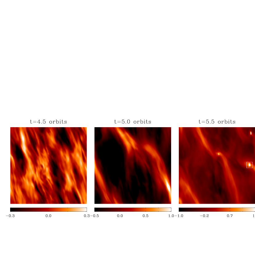
Figure 6: Surface density maps projected on the $x$-$y$ plane of model C. Numbers labeling gray-scale bars correspond to log $\Sigma/\Sigma_{0}$. A square in the right panel indicates the sector viewed as a three-dimensional visualization in Figure 8.

As Figure 1 shows, models C-E with $Q\leq 1.5$ achieve high enough density to produce self-gravitating runaway, while other models with $Q\geq 1.7$ remain stable (with large fluctuations in density). From careful examinations of density power spectra at successive times, we identify the mechanism of self-gravitating cloud formation in models C-E with swing amplification of high-amplitude density perturbations. As discussed in the previous subsection, the power spectra of MRI-driven turbulence peak at small wavenumbers, so that the corresponding large spatial scale density perturbations can be easily swing-amplified if self-gravity is sufficient. Figure 6 shows surface density snapshots at $t/t_{\rm orb}$=4.5, 5.0, and 5.5 of model C (with $Q=1.0$). In the left frame, the maximum power in the surface density is in a trailing $n_{x}=4,n_{y}=1$ mode, but there is also considerable power in a leading mode with $n_{x}=-1$ and $n_{y}=1$. The swing amplifier causes the leading mode to accumulate more mass as it shears into trailing configuration. The net result is the formation of high density filaments (middle frame), which collide with each other and then fragment to form three bound condensations (right frame). At their initial formation, the clumps have mass $M\approx M_{\rm J,2D}\sim 10^{7}{\rm\,M_{\odot}}$ each (see eq. [5]); they subsequently accrete additional material from their surroundings. At the end of the simulation ($t/t_{\rm orb}$=5.5), the mass contained in the three clumps is $\sim 14\%$ of the total mass, corresponding to each clump of mass $\sim 2.2M_{\rm J,2D}$.

Because of its weaker self-gravity, model D with $Q=1.5$ and $\beta(0)=100$ requires two major swing amplification events before its eventual gravitational runaway occurs. In particular, intermediate-density filaments (from the first swing amplification) have $\rho_{\rm max}\approx 4.6\rho_{0}(0)$ at $t/t_{\rm orb}\sim 5$, but these fail to initiate gravitational collapse. Although most of power at this point is in the form of trailing waves, nonlinear interactions of sheared large-amplitude wavelets are vigorous, especially given the stresses from highly turbulent magnetic fields, which ends up supplying fresh small-$|k_{x}|$ modes (Paper I). Another phase of swing amplification follows, this time yielding sufficient enhancement of density to trigger gravitational runaway. Model D forms a bound clump with $M\approx M_{\rm J,2D}$ at the end of the run. The evolution of model E with $Q=1.5$ and $\beta(0)=400$ is quite similar to that of model D, but the lower-amplitude saturated state of MRI when the mean magnetic field is weaker causes the formation of a bound cloud to take longer.

The self-gravitating clouds that form in our simulations turn out all to be magnetically supercritical. For instance, the mass-to-flux ratio of the cloud marked by a square in the left frame of Figure 6 is $M/\Phi_{B}\sim 1.3\,G^{-1/2}$ at $t/t_{\rm orb}=5.1$ when it first appears, and increases to $\sim 3.6\,G^{-1/2}$ at $t/t_{\rm orb}=5.5$, well above the critical value of $\sim 0.13\,G^{-1/2}$ (e.g., Shu 1992). Here, $\Phi_{B}$ denotes the magnetic flux that passes through the cloud and $G$ is the gravitational constant. The other bound clouds also have mass-to-flux ratios in the similar range, that is, $M/\Phi_{B}\sim(1-4)\,G^{-1/2}$, with higher values corresponding to more-evolved, more-massive clouds. Note that the lower limit of this range is remarkably similar to $M/\Phi_{B}\sim 0.96\,G^{-1/2}$ of a square region projected in the $x-y$ plane that contains one Jeans mass in the saturated-MRI disk with the mean $\bar{B}_{y}\sim 2\mu$G. This suggests that the bound clouds initially form by collecting material relatively isotropically in a way that preserves the magnetic flux fairly well. As the clouds become sufficiently self-gravitating, they begin to collapse and accrete more gas in all three dimensions, perhaps with accretion along the mean field direction enhancing the mass-to-flux ratio at later time. Although hard to quantify with our present limited resolution, magnetic reconnection occurring inside the clouds may also contribute to high mass-to-flux ratios.

As Figure 1 clearly illustrates, the threshold for nonlinear gravitational instability in our MRI-driven turbulent galactic disk models is in the range $Q=[1.5,1.7]$. This threshold $Q_{\rm th}$ is higher than found for either completely unmagnetized ($Q_{\rm th}<1$) or thermal-equipartition-magnetized ($Q_{\rm th}\sim 1$) 3D disk models in Paper III. When bound clouds formed in those models, they had masses of two to several $M_{\rm J,2D}$, similar to the present results. We note that in our previous simulations without large-amplitude turbulence, any model with density fluctuations as large as those in model F (see Table 3) ended in gravitational runaway. Here, however, the same turbulence that creates overdense regions can also destroy them, such that model F is nonlinearly gravitationally stable. The MRI-driven turbulent disks have higher $Q_{\rm th}$ than the models of Paper III partly because the turbulence produces large-amplitude, large-scale perturbations in the surface density (see Tables 2,3) that reduce the effective value of $Q$ by $20-40\%$. In addition, torques from small-scale magnetic fields can drive radial angular momentum and mass transport, much as occurs from the MRI in accretion disk models. Since vorticity conservation of fluid elements is the chief barrier to gravitational instability at large enough scales in rotating disks, radial transfer of angular momentum within/across an overdense region can contribute to enabling runaway condensation (cf. Gammie 1996).

3.2.2 Angular Momenta of Condensations

A longstanding astronomical issue of great interest is how the total angular momentum of a self-gravitating cloud evolves as it condenses out of the diffuse ISM. The prevailing idea is that magnetic fields linking a cloud with the surrounding medium exert back-torques as it spins up during contraction, leading to loss of angular momentum (e.g., Gillis, Mestel, & Paris 1974; Mouschovias & Paleologou 1979). Most previous work on this “magnetic braking” process has focused on the problem of an ideal cloud anchored to the ambient medium with a prescribed magnetic field distribution, solving to obtain the temporal evolution of the angular velocity. Using our three-dimensional simulation data from both the present models and those from Paper III, we will demonstrate directly in this subsection that a cloud that condenses out of a rotating, magnetized disk can shed significant angular momentum via magnetic braking during the cloud-forming phase.

To describe the rotational properties of a self-gravitating cloud, we consider the volume bounded by an isodensity surface $\rho=\rho_{\rm crit}$. We define the total angular momentum and the total mass of a volume with $\rho>\rho_{\rm crit}$ as

$$\mathcal{L}_{z}(\rho_{\rm crit})\equiv\int_{\rho>\rho_{\rm crit}}\!\!\!\!\!\rho(xv_{y}-yv_{x})\,d^{3}x,$$ (7)

$$\mathcal{M}(\rho_{\rm crit})\equiv\int_{\rho>\rho_{\rm crit}}\!\!\!\!\!\rho\,d^{3}x,$$ (8)

respectively, where the coordinates ($x$, $y$, $z$) and the inplane velocity ($v_{x}$, $v_{y}$) are measured relative to the center of the condensation. One may then calculate the mean specific angular momentum $J_{z}\equiv\mathcal{L}_{z}/\mathcal{M}$ as a function of $\rho_{\rm crit}$. Because model disks from which bound clouds originate may have different specific angular momenta initially, it is useful to compare $J_{z}$ of a cloud with $J_{\rm gal}$, the total specific angular momentum that the cloud would have if it did not lose any angular momentum during its formation. For a region of uniform surface density, it can be shown that

$$J_{\rm gal}={\Omega\over A}\int[(1-q)x^{2}+y^{2}]d^{2}x$$ (9)

where $A$ is the area of the region in the plane of the disk (cf. Mestel 1966). Thus, in the case of a flat rotation curve $q=1$, $J_{\rm gal}=\Omega L_{0}^{2}/12$ for a square patch of side $L_{0}$ in the unperturbed disk. For purposes of comparison, we shall take $L_{0}$ such that the total mass is the same as that within the $\rho=\rho_{crit}$ surface for the bound cloud that forms.

Exemplary profiles of $J_{z}(\rho_{\rm crit})/J_{\rm gal}$ for three bound clouds at a few selected times are shown in Figure 7. In the figure, “MRI” refers to a cloud that forms within the region marked by a square in the Figure 6 snapshot of model C ($Q=1.0,s_{0}=1$) of this paper, while the curves with “Parker” and “Swing” correspond to clouds formed in magnetized model D ( $Q=0.7,s_{0}=25,\beta=1$) and unmagnetized model C ($Q=0.7,s_{0}=25,\beta=\infty$) of Paper III, respectively. It is apparent that magnetized clouds (“MRI” and “Parker”) lower their specific angular momentum over time as they gravitationally contract, while $J_{z}$ of an unmagnetized cloud (“Swing”) fluctuates around $\sim 0.5J_{\rm gal}$. This implies, consistent with expectations, that magnetic fields play a key role in removing angular momentum. Although the resolution of the present simulations is not sufficient to follow this process over long periods, the characteristic angular momentum loss time during the interval measured is $J_{z}/|\dot{J}_{z}|\sim(1-2)\Omega^{-1}$ for the magnetized models. Since bound clouds typically form within $t_{\rm coll}\sim(1-3)\Omega^{-1}$ (see Fig. 1), the similarity of timescales suggests that magnetic braking is quite efficient, possibly enough to explain the very low observed specific angular momenta of GMCs (e.g., Blitz 1993) compared to their corresponding $J_{\rm gal}$ values.

To help visualize the magnetic braking process that occurs in our simulations, we show in Figure 8 a volumetric rendering of an isodensity surface and magnetic field lines, as well as the density and velocity field at the midplane, for a dense clump in model C at $t/t_{\rm orb}=5.5$. The midplane velocity vectors show that the cloud is counter-rotating with respect to the the sense of the background shear, with the principal rotation axis parallel to the $z$-direction (this sense of spin is prograde with respect to galactic rotation).

The magnetic field lines show rather complex behavior. Some field lines (black) at mid-latitude regions loop back to the cloud, while other field lines anchor the cloud to the ambient medium. Field lines drawn in green start running from the right edge of the box, swirl into the cloud in the counterclockwise direction, and reemerge to swirl in the clockwise direction out to the left edge of the box. These field lines exert net torques on the cloud surface. On the other hand, field lines drawn in blue that touch the ceiling of the box are relatively straight. The fact that the horizontal field lines are more twisted than the vertical field lines suggests that magnetic fields perpendicular to the spin axis provide most of the braking. Although the periodic $z$-boundary conditions we have adopted tend to reduce vertical torsion, an important physical consideration is that there is larger inertia of ambient gas in the horizontal direction (e.g., Mouschovias & Paleologou 1979), tending to promote large horizontal torsion.

Finally, we remark that limited resolution in the current simulations may affect the measured estimate of angular momentum loss. With higher-resolution simulations (employing adaptive or nested meshes), it will be possible to make a more quantitative assessment of how effective magnetic braking is in removing a cloud’s initial angular momentum.

4 Summary and Discussion

Understanding the origins of GMCs is key to characterizing star formation on a galactic scale, because the rate and mode of star formation are linked to the rate of cloud formation and the physical properties of GMCs at birth. Many different galactic-scale processes may affect GMC formation. In this paper, we use 3D MHD simulations to initiate investigation of MRI-driven turbulence in disk galaxies and its role in prompting cloud-forming gravitational instabilities.

Our numerical models represent local portions of shearing and vertically stratified gas disks with initial density profiles determined by the balance between thermal pressure gradients and gaseous self- and external stellar gravity (see §2). The background azimuthal velocity is set to have a local shear rate of $q\equiv-d\ln\Omega/d\ln R=1$, corresponding to a flat rotation curve. Magnetic fields are initially assumed to be purely vertical and uniform, with strength characterized by $\beta(0)=100$ or 400 (see eq. [3]). For simplicity, we have adopted an isothermal equation of state with sound speed $c_{\rm s}=7\,{\rm km\,s^{-1}}$; the corresponding temperature is characteristic of the warm ISM. We evolve disk models of varying surface density parameterized by the Toomre stability parameter $Q$ (see eq. [4]); we consider models with $Q\sim 1-2$. We explore the nonlinear saturation of MRI and the growth and evolution of self-gravitating structures. In particular, we analyze statistical properties of the turbulence, assess the threshold for gravitational instability, and measure the masses and angular momenta of the bound clouds that form. Where appropriate, for comparison we also analyze the data from some models from Paper III.

4.1 Properties of Turbulence

In §3.1 we investigate the characteristics of turbulence initiated and sustained by MRI in non- or weakly self-gravitating models. Despite the differences in the shear parameter, degree of vertical disk compression, and the presence of self-gravity, the statistical properties of the turbulence in our stratified disks are remarkably similar to those in the nonstratified “accretion disk” simulations of HGB. Our models yield saturated-state Shakura & Sunyaev dimensionless $R-\varphi$ stress parameter $\alpha\sim 0.15-0.3$, ratio of the Reynolds to Maxwell stresses $R_{xy}/M_{xy}\approx 0.13$, and ratio of the total stress to magnetic energy density $T_{xy}/E_{B}\approx 0.64$ (see Table 1). The shapes of the turbulent power spectra are also similar to those of HGB. With a level $\alpha\sim 0.2$ (see also Hawley & Krolik 2002) characterizing angular momentum transport and $c_{\rm s}=7\,{\rm km\,s^{-1}}$, the MRI-driven gas accretion time $t_{\rm acc}\sim R^{2}\Omega/(\alpha c_{\rm s}^{2})$ would exceed $10^{11}$ yr at the solar circle.

To quantify the level of turbulence that is driven by MRI in our models, we directly measure the one-dimensional velocity dispersions in each coordinate direction. We find density-weighted velocity dispersions in models with $\beta(0)=100$ are $\sigma_{x}\sim\sigma_{y}\sim(0.4-0.6)c_{\rm s}$ and $\sigma_{z}\sim(0.2-0.3)c_{\rm s}$, with the mean plasma parameter $\bar{\beta}\sim 1-2$ at saturation. With $c_{\rm s}=7\,{\rm km\,s^{-1}}$ and $\rho_{0}(0)=10^{-24}$ g cm^-3, this implies that MRI in the present models produces turbulent levels up to $\sigma_{x}\sim\sigma_{y}\sim 4\,{\rm km\,s^{-1}}$ and $\sigma_{z}\sim 2\,{\rm km\,s^{-1}}$, and RMS magnetic field strength $\bar{B}\sim(1.8-2.3)\mu$G. These magnetic field strengths are similar to estimates in the Milky May and in external galaxies (e.g., Rand & Lyne 1994; Beck 2000, 2002). The velocity dispersions are significantly lower than the observed line widths of $\sim 7\,{\rm km\,s^{-1}}$ and $\sim 11\,{\rm km\,s^{-1}}$, respectively, for the cold and warm H I components in the Solar neighborhood (e.g., Heiles & Troland 2003). Since the thermal linewidth from cold gas is negligible and that from the warm gas (in the stable regime) is $\sim 7\,{\rm km\,s^{-1}}$, the warm and cold phases both have turbulent velocity dispersions $\sim 7\,{\rm km\,s^{-1}}$, significantly larger than the turbulence levels in the present models. For the extended disks of face-on galaxies, radio observations of H I emission linewidths imply $\sigma_{z}\sim 6-10\,{\rm km\,s^{-1}}$ (e.g., Dickey et al. 1990; van Zee & Bryant 1999; Petric & Rupen 2001) for the atomic gas; in the absence of absorption measurements, it is not directly possible to distinguish the turbulent and thermal contributions (or the proportions of warm/cold gas).

Because the level of the velocity fluctuations depends on the mean magnetic flux, one might argue that we could have obtained larger $\sigma$’s, had we adopted larger initial vertical $B$-fields. HGB found, for example, that the saturation magnetic energy density is linearly proportional to $\lambda_{\rm max}$ and thus to the mean value $B_{z}(0)$, or $\beta(0)^{-1/2}$. If the MRI in a single-phase medium is to produce $\sigma_{z}$ up to the observational values, these scalings would imply that the vertical magnetic field should have $\beta(0)\lower 2.15277pt\hbox{$\;\buildrel<\over{\sim}\;$}10$ (assuming that the magnetic and perturbed kinetic energy densities at saturation are also linearly proportional). Equation (6) would then require $\lambda_{\rm max}\lower 2.15277pt\hbox{$\;\buildrel>\over{\sim}\;$}600$ pc for the vertical wavelength of MRI; if this is larger than the thickness of the disk, the saturation energy density would have to be reduced accordingly. Even if larger mean vertical fields were able to produce larger velocity dispersions, the implied total magnetic energy densities would exceed observed values in disk galaxies. Given these constraints, we conclude that MRI acting in a single-phase medium could not generate the level of turbulence implied by H I line width measurements.

It is unknown – but of great interest – whether MRI processes acting in a much less uniform, multi-phase disk could yield appreciably larger velocity dispersions. One might expect, for example, a larger velocity dispersion for a given MRI driving rate if larger effective mean free paths for dissipative interactions in a cloudy medium (compared to a single-phase medium) reduces the turbulent decay rate. Even if the MRI angular momentum transport rate – proportional in steady state to the energy dissipation rate per unit mass $\alpha(P/\bar{\rho})q\Omega$ – increased by a factor $4-9$ for a factor $2-3$ increase in $\sigma_{\rm turb}$ compared to the above, the accretion time ($\propto 1/\alpha$) is still comparable to the Hubble time. This timescale for inflow is long enough to allay the historical concern of overrapid accretion if turbulence taps the orbital energy of the ISM in a galaxy (cf. Spitzer 1968). In addition, the implied volume heating rate would also still be well within the limits set by C II emission from the diffuse ISM (Wolfire et al., 2003). Numerical simulations will be required to decide whether MRI-driven turbulence in a multi-phase medium is competitive with the conventional turbulent energy source for the ISM, supernova shocks (e.g., Cox & Smith 1974; McKee & Ostriker 1977). Initial work towards this goal is already underway (Piontek & Ostriker, 2003). Realistic theoretical assessment of the contributing turbulent driving processes may ultimately require simultaneous modeling, since the dynamical effects are not necessarily independent.

Our three-dimensional simulations show that the enhancement in the amplitudes of velocity fluctuations by the presence of self-gravity is so small (less than 30%) that self-gravity alone is unlikely to be a major source of galactic turbulence for a single-phase disk. Recently, Wada & Norman (1999) and Wada et al. (2002) using two-dimensional hydrodynamic simulations argued that self-gravity can extract sufficient turbulent energy from large-scale galactic rotation to maintain the observed level of turbulence in the ISM. Their conclusion is based on the development of a turbulent velocity field with $\sigma_{\rm turb}\sim 10\,{\rm km\,s^{-1}}$ in thermally and gravitationally unstable flows. At the point a quasi-steady state is reached in the Wada et al. models, most of the gas ($\lower 2.15277pt\hbox{$\;\buildrel>\over{\sim}\;$}80\%$) is contained in cold ($T<100$K) clouds occupying $<1\%$ of the disk area. Thus, the cloudy medium resembles a disk of collisionless particles which has kinetically heated itself through large-scale gravitational instabilities until the typical dispersion in random velocities $\sim 10\,{\rm km\,s^{-1}}$ is sufficient to render $Q_{\rm eff}>1$. These sorts of models are likely appropriate for the ISM in galactic center regions (often dominated by molecular gas) rather than for the ISM in the main and outer disk, where surface densities are an order of magnitude lower than those considered by Wada et al., and where observations indicate that a much smaller proportion of the gas is in cold, dense clouds.

In an application to NGC 2915, Wada et al. (2002) also presented a 2D model that extends up to $R=15$ kpc. They found that rapid cooling of gas makes even very low surface-density disks highly susceptible to thermal and gravitational instability that produces a cloudy medium with $\sigma_{\rm turb}\sim 2-4\,{\rm km\,s^{-1}}$. Combined together with our finding that turbulence driven by self-gravity is not significant as long as the disks are weakly self-gravitating (with $Q\lower 2.15277pt\hbox{$\;\buildrel>\over{\sim}\;$}1.7$) and remain isothermal, this suggests that the dynamical importance of self-gravity may depend strongly on the effective filling factor of the gas. It is therefore essential to run 3D models with a range of properties to determine how the amplitudes of turbulence from self-gravitational driving scale with the relative proportions of cold, dense, and warm (or hot) diffuse gas. These proportions of gas in different phases cannot be tuned directly since turbulence itself can affect the ratio of dense to diffuse gas, via collisional shock heating and other related processes.

4.2 Bound Cloud Formation

In §3.2, we study directly the nonlinear interaction of MRI-driven turbulence with self-gravity, showing that Jeans-mass-scale bound condensations form provided that the mean gas surface density is sufficiently high. In terms of the Toomre parameter, the nonlinear instability condition is $Q<Q_{\rm th}\approx 1.6$. The route to cloud formation is swing amplification of nonlinear density fluctuations ($\delta\rho/\rho\sim 2.3-4.6$) over large spatial scales ($\sim{\rm kpc}$) that arise as a consequence of the MRI. Compared to our previous 3D models of unmagnetized or strongly-magnetized ($\beta=1$) disks which yielded $Q_{\rm th}\lower 2.15277pt\hbox{$\;\buildrel<\over{\sim}\;$}1$ (Paper III), the MRI-unstable disks have larger $Q_{\rm th}$. This higher $Q_{\rm th}$ may partly be because self-gravity is initially strong in the large-amplitude density fluctuations driven by turbulence, enhancing the effectiveness of the swing amplifier; the higher $Q_{\rm th}$ may also owe in part to the ability of small-scale magnetic fields to transfer angular momentum between over- and under-dense regions locally.

The $Q$ threshold we find is similar to the empirical result $Q_{\rm th}\sim 1.4$ obtained by Martin & Kennicutt (2001) based on azimuthally-averaged gas surface densities in a large sample of galaxies. Although intriguing, we caution that this close coincidence may be particular to the details of the current models (e.g. the net poloidal magnetic flux, the phase state of the gaseous medium). Nevertheless, we consider it a significant success that theory and observation have arrived at essentially the same simple criterion for the onset of active star formation in galactic disks.

Gravitationally bound clouds that form in our simulations are all magnetically supercritical with the mass-to-flux ratio of $M/\Phi_{B}\sim(1-4)G^{-1/2}$ and have typical masses of a few $10^{7}{\rm\,M_{\odot}}$ each, corresponding roughly to the two-dimensional Jeans mass at the mean surface density. These clouds have masses consistent with the largest atomic or molecular clouds found in disk galaxies (e.g., Elmegreen & Elmegreen 1983; Vogel et al. 1988; Rand & Kulkarni 1990; Sakamoto et al. 1999). The molecular components of the largest Milky Way GMCs are nearly an order of magnitude lower in mass. The added contribution from H I, which increases total masses of Milky Way GMCs by at least a factor of two (Blitz, 1993), reaching $\lower 2.15277pt\hbox{$\;\buildrel>\over{\sim}\;$}10^{7}{\rm\,M_{\odot}}$ in some cases (e.g., Elmegreen & Elmegreen, 1987), accounts for some of the disparity between our present results and observed molecular clouds. In addition, the disparity may owe in part to expected differences between cloud masses in systems with and without strong spiral structure, as discussed below.

Table 4 summarizes the model prescription/parameters and main results for bound cloud formation from Papers I-III and the present work. As Table 4 indicates, our simulations so far have considered both disk models without features in the background gravitational potential (Paper I in 2D; Paper III and this work in 3D), and disk models that include a background (stellar) spiral potential (Paper II in 2D). All of our models to date are local.

Although restricted to the 2D razor-thin limit, Paper II demonstrated that when spiral structure is present, gravitational instabilities (in particular, the MJI) form clouds preferentially in spiral arm regions, consistent with the observations that the warmest, most massive GMCs in the Milky Way are strongly correlated with spiral structure (e.g., Solomon et al. 1985; Dame et al. 1986; Solomon & Rivolo 1989). While the mean gaseous surface densities for models that formed clouds in Paper I (without spiral structure) and Paper II (with spiral structure) were similar, the resulting cloud masses in Paper II were smaller by a factor $\sim 5-7$. This difference owes to the overall compression of diffuse gas in spiral arms, which reduces the Jeans mass $\propto\Sigma^{-1}$; the mass collection zone is also limited by the width of the spiral arm itself.

For a given gaseous surface density, cloud masses are also affected by the thickness of the disk, since increasing the thickness dilutes self-gravity, typically increasing the in-plane Jeans length by a factor $\sim 2$. With weaker self-gravity, a larger total area/mass is needed to prompt instability. Thus, the 3D models of Paper III produced larger cloud masses at given surface density (i.e. $Q$ value) than would have been predicted on the basis of the 2D models of Paper I (although since instability was present only for smaller $Q$ in 3D than in 2D, the resulting cloud masses in Papers I, III were similar).

Real galactic disks of course have finite thickness and are turbulent, and in this sense the current models supersede the “swing” models of Papers I and III. However, real galaxies also in general contain stellar spiral structure, which Paper II implemented only in 2D. Finite thickness effects are expected to increase the cloud spacings and masses that form by MJI in spiral arms compared to the results of Paper II. Although this could imply up to a factor $\sim 4$ increase in cloud masses at a given surface density, turbulence could limit this increase somewhat. Three-dimensional simulations with explicit modeling of spiral potential perturbations and vertical density stratification are required to address this and related questions directly, although our net expectations from effects currently studied suggest total cloud masses in the neighborhood of $10^{7}{\rm\,M_{\odot}}$.

Because observed GMCs have very small specific angular momenta (Blitz, 1993) compared to galactic values (see eq. [9]) on comparable mass scales, it is of much interest to determine when and how this angular momentum is lost. Using our models, we explicitly demonstrate that a self-gravitating, contracting, magnetized cloud loses specific angular momentum via surface torques imposed by the large-scale galactic magnetic fields that thread it. This magnetic braking is predominantly from horizontal $B$-fields (perpendicular to the spin axis of the cloud) that connect the cloud to the dense portion of the galactic disk. Our preliminary estimates suggest that the rate of angular momentum loss is sufficient to explain observations of low GMC spins, although higher-resolution simulations will be needed to confirm this result.

Finally, we remark on the mass spectrum of Galactic molecular clouds, generally described from CO observations as a power-law $dN/dM\propto M^{-1.6}$ below a cutoff of a few $\times 10^{6}{\rm\,M_{\odot}}$ (e.g., Solomon et al. 1987) (with H I envelopes increasing individual cloud masses by factors of $2-10$). The gravitational instability scenario of this work and Papers I-III explains the upper cutoff in terms of the Jeans mass, as noted above (see also e.g. Elmegreen 1979, 1994). Below this cutoff, the mass spectrum may mainly reflect the effects of turbulent dynamics within massive (Jeans-scale) clouds as they form and subsequently disperse. Recent analysis of simulated models of turbulent GMCs has shown that a power-law spectrum of moderate-density clumps develops (Ostriker, 2002); the index measured is the same as the observed Galactic cloud spectrum. If the processes that disperse a GMC preserve the mass spectrum of former clumps as isolated clouds, and/or if observational identification methods decompose some large GMCs into their sub-parts, then similar clump and cloud mass spectra are a natural consequence of “top-down” GMC formation.

Table 1: Parameters of Three-Dimensional Simulations

Model (1)	$Q$ (2)	$\beta(0)$ (3)	Gravity (4)	Results (5)	$R_{xy}/M_{xy}$ (6)	$T_{xy}/E_{B}$ (7)	$\sigma_{x}/c_{\rm s}$ (8)	$\sigma_{y}/c_{\rm s}$ (9)	$\sigma_{z}/c_{\rm s}$ (10)
A	1.5	100	no	…	0.13	0.64	0.45	0.43	0.23
B	1.5	400	no	…	0.14	0.65	0.21	0.21	0.13
C	1.0	100	yes	unstable	…	…	…	…	…
D	1.5	100	yes	unstable	…	…	…	…	…
E	1.5	400	yes	unstable	…	…	…	…	…
F	1.7	100	yes	stable	0.14	0.62	0.58	0.50	0.30
G	2.0	100	yes	stable	0.13	0.64	0.58	0.50	0.32

Table 2: Volume- and Time- Averaged Quantities in Model A

Quantity	$\langle\langle f\rangle\rangle$	$\langle\langle\delta f^{2}\rangle\rangle^{1/2}$	min $f$	max $f$
$B_{x}/(4\pi P_{0}(0))^{1/2}$	2.39$\times 10^{-7}$	0.326	$-1.362$	1.317
$B_{y}/(4\pi P_{0}(0))^{1/2}$	$-1.30\times 10^{-4}$	0.576	$-1.550$	1.467
$B_{z}/(4\pi P_{0}(0))^{1/2}$	0.1000	0.174	$-0.898$	1.189
$B_{x}^{2}/8\pi P_{0}(0)$	0.0532	0.072	0.000	0.957
$B_{y}^{2}/8\pi P_{0}(0)$	0.1808	0.147	0.000	1.218
$B_{z}^{2}/8\pi P_{0}(0)$	0.0196	0.035	0.000	0.691
$-B_{x}B_{y}/4\pi P_{0}(0)$	0.1435	0.168	$-$0.880	1.323
$-B_{x}B_{z}/4\pi P_{0}(0)$	$-$0.0012	0.075	$-$0.850	0.838
$-B_{y}B_{z}/4\pi P_{0}(0)$	0.0031	0.110	$-$0.885	0.913
$\rho v_{x}^{2}/2P_{0}(0)$	0.0334	0.062	0.000	1.557
$\rho\delta v_{y}^{2}/2P_{0}(0)$	0.0293	0.065	0.000	1.687
$\rho v_{z}^{2}/2P_{0}(0)$	0.0116	0.023	0.000	0.718
$\rho v_{x}\delta v_{y}/P_{0}(0)$	0.0180	0.088	$-$1.011	1.760
$\rho v_{x}v_{z}/P_{0}(0)$	0.0005	0.050	$-$1.250	0.883
$\rho\delta v_{y}v_{z}/P_{0}(0)$	0.0008	0.050	$-$1.050	1.090
$P_{\rm tot}/P_{0}(0)$	0.5863	0.396	0.029	2.478
$\rho/\rho_{0}(0)$	0.3320	0.338	0.000	2.184
$(\rho-\rho_{0})/\rho_{0}(0)$	0.0000	0.184	$-$0.851	1.233
$\Sigma/\Sigma_{0}$	1.0000	0.201	0.474	1.779

Table 3: Volume- and Time- Averaged Quantities in Model F

Quantity	$\langle\langle f\rangle\rangle$	$\langle\langle\delta f^{2}\rangle\rangle^{1/2}$	min $f$	max $f$
$B_{x}^{2}/8\pi P_{0}(0)$	0.0767	0.108	0.000	1.879
$B_{y}^{2}/8\pi P_{0}(0)$	0.3138	0.215	0.000	2.076
$B_{z}^{2}/8\pi P_{0}(0)$	0.0230	0.045	0.000	0.966
$-B_{x}B_{y}/4\pi P_{0}(0)$	0.2252	0.249	$-$1.378	2.538
$-B_{x}B_{z}/4\pi P_{0}(0)$	$-$0.0008	0.104	$-$1.351	1.412
$-B_{y}B_{z}/4\pi P_{0}(0)$	0.0030	0.164	$-$1.468	1.483
$\rho v_{x}^{2}/2P_{0}(0)$	0.0566	0.117	0.000	3.088
$\rho\delta v_{y}^{2}/2P_{0}(0)$	0.0412	0.111	0.000	3.398
$\rho v_{z}^{2}/2P_{0}(0)$	0.0167	0.033	0.000	0.888
$\rho v_{x}\delta v_{y}/P_{0}(0)$	0.0310	0.156	$-$2.307	3.544
$\rho v_{x}v_{z}/P_{0}(0)$	0.0023	0.082	$-$1.491	1.928
$\rho\delta v_{y}v_{z}/P_{0}(0)$	0.0013	0.074	$-$1.669	1.790
$P_{\rm tot}/P_{0}(0)$	0.7461	0.482	0.046	5.474
$\rho/\rho_{0}(0)$	0.3320	0.399	0.000	5.068
$(\rho-\rho_{0})/\rho_{0}(0)$	0.0000	0.292	$-$0.962	4.093
$\Sigma/\Sigma_{0}$	1.0000	0.410	0.310	3.493

Table 4: Summary of Papers I-III and the present work

paper	disk geometry	background feature	magnetic field	instability threshold and outcome	physical mechanism
paper I	razor thin	none	azimuthal	$Q_{c}=1.2-1.4$	high shear: Swing
	disks (2D)		$(\beta_{y}=\infty,10,1)$	$M_{\rm cloud}$ = a few $10^{7}{\rm\,M_{\odot}}$	low shear: MJI
paper II	razor thin	spiral	azimuthal	$M_{\rm cloud}=4\times 10^{6}{\rm\,M_{\odot}}$	MJI inside
	disks (2D)	arms	$(\beta_{y}=\infty,10,1)$		spiral arms
paper III	finite thickness	none	azimuthal	$Q_{c}\lower 2.15277pt\hbox{$\;\buildrel<\over{\sim}\;$}1.0$	Swing; MJI with
	disks (3D)		$(\beta_{y}=\infty,1)$	$M_{\rm cloud}$ = a few $10^{7}{\rm\,M_{\odot}}$	Parker-driven boost
this paper	finite thickness	none	vertical	$Q_{c}=1.6$	Swing of MRI-driven
	disks (3D)		$(\beta_{z}=100,400)$	$M_{\rm cloud}$ = a few $10^{7}{\rm\,M_{\odot}}$	turbulence

Figure 1: Time evolution of maximum density (solid lines) and density dispersion (dotted lines) of (a) $\beta=100$ and (b) $\beta=400$ models. The dashed line in (a) represents the linear growth rate of the most unstable MRI mode for the parameters of non-self-gravitating model A.

Figure 2: Gray-scale images of the perturbed density $\delta\rho/\rho_{0}(0)$ at four time epochs from model A. Each frame (a)-(d) displays slices at $y=-L_{y}/2$ (left; $x-z$ plane) and $x=-L_{x}/2$ (right; $y-z$ plane). The MRI “channel solution” that appears strongly at $t/t_{\rm orb}=3$ (frame [b]) breaks up and generates MHD turbulence at $t/t_{\rm orb}\lower 2.15277pt\hbox{$\;\buildrel>\over{\sim}\;$}4$ (frames [c],[d]).

Figure 3: Vertical variations of horizontally averaged quantities in model A. The dimensionless, differential surface element $dS$ is defined by $dS\equiv dxdy/(L_{x}L_{y})$. (a) The averaged density distribution remains close to the initial profile even when turbulence is fully developed. (b) In the saturated state, $\beta$ is reduced to $\sim 1-10$ at $|z|/H\lower 2.15277pt\hbox{$\;\buildrel<\over{\sim}\;$}2$. In (c), the magnetic energy density dominates the total energy density, and in (d), the Maxwell stress dominates the total $x-y$ (radial-azimuthal) stress.

Figure 5: Amplitudes of the power spectra along the $k_{x}$, $k_{y}$, and $k_{z}$ axes of density (left) and azimuthal magnetic field (right), averaged over $t/t_{\rm orb}=5-6$, in model A. Along each axis, modes indicated by different lines are as follows: for $k_{x}$, $n_{y}=n_{z}=0$ (solid), $n_{y}=1,n_{z}=0$ (dotted), $n_{y}=0,n_{z}=1$ (dashed), $n_{y}=n_{z}=1$ (dot-dashed); for $k_{y}$, $n_{x}=n_{z}=0$ (solid), $n_{x}=1,n_{z}=0$ (dotted), $n_{x}=0,n_{z}=1$ (dashed), $n_{x}=n_{z}=1$ (dot-dashed); for $k_{z}$, $n_{x}=n_{y}=0$ (solid), $n_{x}=1,n_{y}=0$ (dotted), $n_{x}=0,n_{y}=1$ (dashed), $n_{x}=n_{y}=1$ (dot-dashed), where $n_{x}\equiv k_{x}/2\pi L_{x}$, $n_{y}\equiv k_{y}/2\pi L_{y}$, and $n_{z}\equiv k_{z}/2\pi L_{z}$. For comparison, the slope of the Kolmogorov spectrum ($\sim k^{-11/3}$) is indicated in each pane.

Figure 7: (a) Mean specific angular momenta $J_{z}$ inside surfaces defined by critical density $\rho_{\rm crit}$ of self-gravitating clouds in three-dimensional simulations. For each cloud, $J_{z}$ is normalized to $J_{\rm gal}$ (see eq. [9]), the total specific angular momentum that the cloud would retain if angular momentum were conserved during quasi-isotropic formation. MRI indicates model C in the present work, while Parker and Swing refer to magnetized model D and unmagnetized model C of Paper III, respectively. Note that the magnetized clouds clearly lose specific angular momenta as they collapse, while the unmagnetized model does not.

Figure 8: Perspective visualization of an isodensity surface ($\rho/\rho_{0}(0)=10$) and selected magnetic field lines in model C at $t/t_{\rm orb}=5.5$. The region fits in the projected square marked in Figure 6, with a vertical extent of $|z|<0.04L_{z}$. The magnetic field lines in green run from the right edge of the box into the clump and from the clump to the left edge, while blue indicates field lines that extend to the ceiling of the box. Field lines that return back to the clump are drawn in black. The midplane density slice is shown in colorscale at the bottom of the box (colorbar labels $\log\rho/\rho_{0}(0)$); horizontal velocity vectors in the same plane are also drawn.

References

- Balbus & Hawley (1991) Balbus, S. A., & Hawley, J. F. 1991, ApJ, 376, 214
- Balbus & Hawley (1998) Balbus, S. A., & Hawley, J. F. 1998, Rev. Mod. Phys., 70, 1
- Beck (2000) Beck, R. 2000, in “The Astrophysics of Galactic Cosmic Rays”, eds. R. Diehl et al., Space Science Reviews, (Dordrecht:Kluwer)
- Beck (2002) Beck, R. 2002, in “From Observations to Self-Consistent Modeling of the ISM in Galaxies”, eds. M. Avillez & D. Breitschwerdt, Kluwer Astrophys. & Space Sci. Ser.
- Blitz (1993) Blitz, L. 1993, in Protostars and Planets III, ed. E. Levy & J. Lunine (Tucson: University of Arizona Press), 125
- Blitz & Shu (1980) Blitz, L., & Shu, F. H. 1980, ApJ, 238, 148
- Cox & Smith (1974) Cox, D. P., & Smith, B. W. 1974, ApJ, 189, 105
- Dame et al. (1986) Dame, T. M., Elmegreen, B. G., Cohen, R. S., & Thaddeus, P. 1986, ApJ, 305, 892
- Dickey et al. (1990) Dickey, J. M., Hanson, M. M., & Helou, G. 1990, ApJ, 352, 522
- Elmegreen (1987) Elmegreen, B. G. 1987, ApJ, 312, 626
- Elmegreen (1979) Elmegreen, B.G. 1979, ApJ, 231, 372
- Elmegreen (1989) Elmegreen, B. G. 1989, ApJ, 344, 306
- Elmegreen (1994) Elmegreen, B.G. 1994, ApJ, 433, 39
- Elmegreen (1995) Elmegreen, B. G. 1995, in The 7th Guo Shoujing Summer School on Astrophysics: Molecular Clouds and Star Formation, eds. C. Yuan & Hunhan You (Singapore: World Scientific), 149
- Elmegreen & Elmegreen (1983) Elmegreen, B. G., & Elmegreen, D. M. 1983, MNRAS, 203, 31
- Elmegreen & Elmegreen (1987) Elmegreen, B. G., & Elmegreen, D. M. 1987, ApJ, 320, 182
- Ferguson et al. (1998) Ferguson, A. M. N., Wyse, R. F. G., Gallagher, J. S., & Hunter, D. A. 1998, AJ, 116, 673
- Gammie (1996) Gammie, C. F. 1996, ApJ, 462, 725
- Gammie (2001) Gammie, C. F. 2001, ApJ, 553, 174
- Gillis, Mestel, & Paris (1974) Gillis, J., Mestel, L., & Paris, R. B. 1974, Ap. Space Sci., 27, 167
- Goldreich & Lynden-Bell (1965a) Goldreich, P., & Lynden-Bell, D. 1965a, MNRAS, 130, 97
- Goldreich & Lynden-Bell (1965b) Goldreich, P., & Lynden-Bell, D. 1965b, MNRAS, 130, 125
- Goodman & Xu (1994) Goodman, J., & Xu, G. 1994, ApJ, 432, 213
- Hawley & Balbus (1991) Hawley, J. F., & Balbus, S. A. 1991, ApJ, 376, 223
- Hawley, Gammie, & Balbus (1995) Hawley, J. F., Gammie, C. F., & Balbus, S. A. 1995, ApJ, 440, 742 (HGB)
- Hawley, Gammie, & Balbus (1996) Hawley, J. F., Gammie, C. F., & Balbus, S. A. 1996, ApJ, 464, 690
- Hawley & Krolik (2002) Hawley, J. F., & Krolik, J. H. 2002, ApJ, 566, 164
- Heiles & Troland (2003) Heiles, C., & Troland, T. H. 2003, ApJ, 586, 1067
- Heitsch, Mac Low, & Klessen (2001) Heitsch, F., Mac Low, M.-M., & Klessen, R. S. 2001, ApJ, 547, 280
- Heyer & Terebey (1998) Heyer, M. H., & Terebey, S. 1998, ApJ, 502, 265
- Holmberg & Flynn (2000) Holmberg, J., & Flynn, C. 2000, MNRAS, 313, 209
- J.Kim et al. (2000) Kim, J., Franco, J., Hong, S. S., Santillán, A., & Martos, M. A. 2000, ApJ, 531, 873
- J.Kim et al. (2001) Kim, J., Ryu, D., & Jones, T. W. 2001, ApJ, 557, 464
- Kim & Ostriker (2000) Kim, W.-T., & Ostriker, E. C. 2000, ApJ, 540, 372
- Kim & Ostriker (2001) Kim, W.-T., & Ostriker, E. C. 2001, ApJ, 559, 70 (Paper I)
- Kim & Ostriker (2002) Kim, W.-T., & Ostriker, E. C. 2002, ApJ, 570, 132 (Paper II)
- Kim, Ostriker, & Stone (2002) Kim, W.-T., Ostriker, E. C., & Stone, J. M., 2002, ApJ, 581, 1080 (Paper III)
- Kuijken & Gilmore (1989) Kuijken, K., & Gilmore, G. 1989, MNRAS, 239, 605
- Lynden-Bell (1966) Lynden-Bell, D. 1966, Observatory, 86, 57
- Martin & Kennicutt (2001) Martin, C. L., & Kennicutt, R. C., Jr. 2001, ApJ, 555,301
- McKee & Ostriker (1977) McKee, C. F., & Ostriker, J. P. 1977, ApJ, 218, 148
- Mestel (1966) Mestel, L. 1966, MNRAS, 131, 307
- Miller & Stone (2000) Miller, K. A., & Stone, J. M. 2000, ApJ, 534, 398
- Mouschovias & Paleologou (1979) Mouschovias, T. Ch., & Paleologou, E. V. 1979, ApJ, 230, 204
- Mouschovias, Shu, & Woodward (1974) Mouschovias, T. Ch., Shu, F. H., & Woodward, P. R. 1974, A&A, 33, 73
- Ostriker (2002) Ostriker, E. C. 2002, in Simulations of Magnetohydrodynamic Turbulence in Astrophysics” eds. T. Passot & E. Falgarone (Springer)
- Ostriker, Stone, & Gammie (2001) Ostriker, E. C., Stone, J. M., & Gammie, C. F. 2001, ApJ, 546, 980
- Petric & Rupen (2001) Petric, A., & Rupen, M. 2001, in Gas and Galaxy Evolution, ASP Conf. Ser. 240, eds. J. E. Hibbard, M. P. Rupen, & J. H. van Gorkom, p. 288
- Piontek & Ostriker (2003) Piontek, R.A., & Ostriker, E.C. 2003, ApJ, submitted
- Rand (1993) Rand, R. J. 1993, ApJ, 410, 68
- Rand & Kulkarni (1990) Rand, R. J., & Kulkarni, S. R. 1990, ApJ, 349, L43
- Rand & Lyne (1994) Rand, R. J., & Lyne, A. G. 1994, MNRAS, 268, 497
- Rix & Zaritsky (1995) Rix, H. W., & Zaritsky, D. 1995, ApJ, 447, 82
- Sakamoto et al. (1999) Sakamoto, K., Okumura, S. K., Ishizuki, S., & Scoville, N. Z. 1999, ApJS, 124, 403
- Sellwood and Balbus (1999) Sellwood, J. A., & Balbus, S. A. 1999, ApJ, 511, 660
- Shakura & Sunyaev (1973) Shakura, N. I., & Sunyaev, R. A. 1973, A&A, 24, 337
- Shu (1992) Shu, F. H. 1992, The Physics of Astrophysics. II. Gas Dynamics (Mill Valley: Univ. Science Books), 335
- Solomon et al. (1985) Solomon, P. M., Sanders, D. B., & Rivolo, A. R. 1985, ApJ, 292, L19
- Solomon et al. (1987) Solomon, P. M., Rivolo, A. R., Barrett, J., & Yahil, A. 1987, ApJ, 319, 730
- Solomon & Rivolo (1989) Solomon, P. M., & Rivolo, A. R. 1989, ApJ, 339, 919
- Spitzer (1968) Spitzer, L., Jr. 1968, in Nebulae and Interstellar Matter, eds. B. Middlehurst & L. Aller, (U. Chicago Press), 1
- Stone & Norman (1992a) Stone, J. M, & Norman, M. L. 1992a, ApJS, 80, 753
- Stone & Norman (1992b) Stone, J. M, & Norman, M. L. 1992b, ApJS, 80, 791
- Stone et al. (1996) Stone, J. M., Hawley, J. F., Gammie, C. F., & Balbus, S. A. 1996, ApJ, 463, 656 (SHGB)
- Stone, Ostriker, & Gammie (1998) Stone, J. M., Ostriker, E. C., & Gammie, C. F. 1998, ApJ, 508, L99
- Stone et al. (2000) Stone, J. M., Gammie, C. F., Balbus, S. A., & Hawley, J. F. 2002, in Protostars and Planets IV, ed. V. Mannings, A. P. Boss, & S. S. Russell (Tuscon:Univ. of Arizona press), 589
- Toomre (1964) Toomre, A. 1964, ApJ, 139, 1217
- Toomre (1981) Toomre, A. 1981, in Structure and Evolution of Normal Galaxies, eds. S. M. Fall & D. Lynden-Bell (Cambridge: Cambridge Univ. Press), 111
- van Zee & Bryant (1999) van Zee, L., & Bryant, J. 1999, AJ, 118, 2172
- Vogel et al. (1988) Vogel, S. N., Kulkarni, S. R., & Scoville, N. Z. 1988, Nature, 334, 402
- Wada & Norman (1999) Wada, K., & Norman, C. A. 1999, ApJ, 516, L13
- Wada et al. (2002) Wada, K., Meurer, G., & Norman, C. A. 2002, ApJ, 577, 197
- Wolfire et al. (2003) Wolfire, M. G, McKee, C. F., Hollenbach, D., & Tielens, A. G. G. M. 2003, ApJ, 587, 278