Measuring the matter distribution within $z=0.2$ cluster lenses with XMM-Newton

Abstract

We present an analysis of $7$ clusters observed by XMM-Newton as part of our survey of $17$ most X-ray luminous clusters of galaxies at $z\sim 0.2$ selected for a comprehensive and unbiased study of the mass distribution in massive clusters. Using the public software FTOOLS and XMMSAS we have set up an automated pipeline to reduce the EPIC MOS & pn spectro-imaging data, optimized for extended sources analysis. We also developped a code to perform intensive spectral and imaging analysis particularly focussing on proper background estimate and removal. XMM-Newton deep spectro-imaging of these clusters allowed us to fit a standard $\beta$-model to their gas emission profiles as well as a standard MEKAL emission model to their extracted spectra, and test their inferred characteristics against already calibrated relations.

INTRODUCTION

Being the most massive gravitationally bound objects in the Universe, clusters of galaxies are prime targets for studies of structure formation and evolution.

Of particular interest are the most X-ray luminous clusters. Indeed, it has been convincingly demonstrated that high X-ray luminosity is a reliable indicator of cluster mass (e.g. [Allen, 1998]). Therefore, X-ray selected clusters samples (e.g. [Ebeling et al., 1996]) are the best choice for undertaking representative studies of the mass distribution in massive, X-ray luminous clusters. In particular, as they are easily detected out to very large redshift, we can hope to probe cluster evolution back from early epochs. However, X-ray luminosity is also sensitive to the presence of cooling flows, mergers and non-thermal effects, thus the Luminosity-Mass and Temperature-Mass relation needs to be clearly understood before any strong ascertion is made on cluster evolution ([Smith et al., 2003]). Proper mass estimate is likely to arise only by combining multiwavelength observations of clusters of galaxies: namely strong and weak lensing observations ([Smith et al., 2001]), velocity distribution and dynamics of the cluster galaxies (in a similar way as in [Czoske et al., 2001]) and through accurate, spatially resolved X-ray temperature measurements as we are concentrating on here.

Following this premise, we are conducting a survey (Table 1) of the most X-ray luminous clusters ($L_{X_{[0.1-2.4~{}keV]}}\geq 8~{}10^{44}~{}erg\cdot s^{-1}$) in a narrow redshift slice at $z\sim 0.2$, selected from the XBACS (X-ray Brightest Abell-type Clusters Sample; [Ebeling et al., 1996]). As XBACS is restricted to Abell clusters ([Abell, Corwin & Olowin, 1989]), it is X-ray flux limited but not truly X-ray selected. However, a comparison with the X-ray selected ROSAT BCS (Brightest Cluster Sample, [Ebeling et al., 2000]) shows that $\sim 75\%$ of the BCS clusters in the redshift and X-ray luminosity range of our sample are in fact Abell clusters. Hence, our XBACS subsample is, in all practical aspects, indistinguishable from an X-ray selected sample.

Table 1: Our cluster list sorted by right ascension. Redshift, Hydrogen column density, flux and luminosity (columns 3 to 6 resp.) are quoted from the XBACS updated database. Out of these 17 clusters, 8 have HST/WFPC2 observations performed (as part of cycle 8 [ID:8249, PI:Kneib]); 3 only have a shallow HST observation through a snapshot survey (8301 & 8719 programmes, PI:Edge); 2 have not yet been observed with HST; the remaining 4 having archival data. Moreover, 11 have been observed in 1999/2000 with the wide field CFH12K camera ([Czoske et al., 2003]). The last column shows the effective exposure duration (after flares removal) for clusters already observed by XMM-Newton (resp. MOS and pn instruments), or quote the priority level within our proposal for those not yet observed.

ID	$\alpha$	$\delta$	$z$	$N_{H}$	$f_{xbacs}$	$L_{xbacs}$	HST	CFH	XMM-Newton
	$J2000$	$J2000$		$10^{20}~{}cm^{-2}$	$10^{-12}~{}cgs$	$10^{44}~{}erg/s$	cycle	semester	$ks$ (MOS/pn)
A68	$00~{}37~{}06$	$+09~{}09~{}20$	0.2546	4.77	5.55	14.90	8249	99-II	22/10
A115	$00~{}55~{}55$	$+26~{}22~{}14$	0.1971	5.39	8.99	14.57	-	-	C
A209	$01~{}31~{}53$	$-13~{}36~{}47$	0.2060	1.56	7.55	13.38	8249	99-II	17/11
A267	$01~{}52~{}41$	$+01~{}00~{}43$	0.2300	2.84	6.21	13.67	8249	99-II	17/12
A383	$02~{}48~{}03$	$-03~{}31~{}04$	0.1871	4.06	5.50	8.09	8249	99-II	25/07
A773	$09~{}17~{}52$	$+51~{}43~{}38$	0.2170	1.34	6.36	12.50	8249	-	15/15
A963	$10~{}17~{}03$	$+39~{}02~{}56$	0.2060	1.40	5.78	10.27	8249	99-I	24/16
A1423	$11~{}57~{}17$	$+33~{}36~{}39$	0.2130	1.66	5.22	9.92	8719	-	C
A1682	$13~{}06~{}49$	$+46~{}33~{}35$	0.2260	1.36	5.44	11.59	8719	-	C
A1689	$13~{}11~{}29$	$-01~{}20~{}31$	0.1840	1.80	14.60	20.64	6004	00-I	AO1 J.Hugues
A1763	$13~{}35~{}19$	$+40~{}59~{}56$	0.2279	0.84	6.54	14.13	8249	99-II	observed
A1835	$14~{}01~{}02$	$+02~{}52~{}03$	0.2528	2.24	14.58	38.24	8249	99-I	PV (27/23)
A2111	$15~{}39~{}42$	$+34~{}25~{}03$	0.2290	2.07	5.01	10.97	-	-	C
A2218	$16~{}35~{}54$	$+66~{}13~{}00$	0.1750	3.20	7.3	17.99	5701, 8500	00-I	GT M.Turner
A2219	$16~{}40~{}20$	$+46~{}42~{}27$	0.2281	1.73	9.23	19.89	6488	00-I	GT M.Turner
A2261	$17~{}22~{}27$	$+32~{}07~{}53$	0.2240	3.36	8.72	18.15	8301	-	AO1 J.Hughes
A2390	$21~{}53~{}37$	$+17~{}41~{}45$	0.2310	6.70	9.50	21.25	5352	00-I	GT M.Watson

THE ANALYSIS PIPELINE

As to the version 5.2 of the official XMM-Newton data analysis software (XMMSAS), the extended sources could not be handled properly, regarding the background subtraction and vignetting corrections. The development of methods, where weights are applied to events according to their energies and positions as well as calibration data so as to correct the event list as if the instrument response were uniformely identical to the on-axis response, started as soon as 2001 ([Arnaud et al., 2001, Majerowicz et al., 2002, Marty et al., 2002, Marty et al., 2003]). We concentrated on our side to embedding these algorithms into an environment capable of pipeline processing a series of data from clusters of galaxies observations. Indeed, the manual operation of XMMSAS (using either external correction routines or integrated algorithms from versions 5.3 and later) is extremely time-consuming: several days for each dataset.

Thanks to our pipeline, we reduced the required time down to less than $10~{}h$ per dataset, adding a working day for eye-inspection of the full sample results and another for compilation and final manual calculations.

This pipeline integrates the latest calibration data from the EPIC consortium as well as specific fitting routines written in IDL and XSPEC environments. It is fully configurable to allow eye-inspection and partial or total re-runs if needed. It is extensively detailed by [Marty et al., 2003], but useful information about “blank” and “dark” fields (for background estimation and subtraction) are also respectively given by [Lumb et al., 2002, Marty et al., 2002]. The general processing scheme is the following:

$\bullet$	re-process each cluster raw data to account for latest calibration knowledge;
$\bullet$	re-project “blank” and/or “dark” data onto telescope aspect solution used for each cluster;
$\bullet$	extract valid events within good-time-intervals (to reject noise and proton flares);
$\bullet$	detect and mask out spurious components (field sources and remaining bad pixels);
$\bullet$	weight the events according to calibration data;
$\bullet$	find the best cluster centroid;
$\bullet$	process radial brightness profiles and fit a standard $\beta$-model convolved by the instrument PSF;
$\bullet$	process full maps in physical flux units and adaptively smooth according to PSF description;
$\bullet$	process spectra and call XSPEC for fitting (global for the mean temperature, annuli for the profile);
$\bullet$	compute hardness maps and derive another temperature profile.

THE PIPELINE RESULTS

Surface brightness profiles

The core radius $R_{c}$, power index $\beta$, normalization $f_{0}$ and background constant $BKG$ are coming from the standard $\beta$-model fitting. Note that the surface brightness profiles have been extracted between $0.3$ and $6.3~{}keV$, logarithmically rebinned to enhance their signal-to-noise ratios and that the inner $40~{}arcsec$ of each cluster profile have been ignored for the fit so as to avoid fitting any emission excess, associated for example to a cooling flow. The background subtraction concerned only the instrumental component so that the $BKG$ constant is a measure of the sky X-ray emission background. The $\beta$-models are convolved by the instrument PSF before fitting.

The $R_{1\sigma}$ parameter is a measure of the radius inside which the cluster signal-to-noise ratio is greater than $1$. The $F_{X}(data)$ and $F_{X}(model)$ parameters then are the integrated fluxes within this detection limit radius, from the data and from the best fit $\beta$-model; in each case, these fluxes are cleaned from the sky background component; the difference between them thus shows the contribution of any excess emission.

Surface brightness maps

Surface brightness maps that have been produced in the same energy band during the pipeline analysis are not presented herein, because of room restrictions and because they are not necessary for the following calculations. However, they may be found on the internet if so desired.

Spectral analysis

Spectra are extracted in the $0.2$ to $12.0~{}keV$ band and rebinned according the Poisson statistics requirements (at least $25$ net counts per bin). They are background subtracted from both instrumental components (estimated using the “closed” data) and sky components (from a spectrum extracted in a peripheral annulus of each dataset, between the $600$ and $800~{}arcsec$ radii) and then fitted against the $TBabs\times MEKAL$ photo-absorption and bremsstrahlung models.

The redshifts $z$ and hydrogen column densities $N_{H}$ have been respectively fixed to the same optical redshift references as used in the original XBACS database, and to the weighted means of the $N_{H}$ measurements from the [Dickey & Lockman, 1990] database included within $1\deg$ of the cluster center. The resulting temperatures $kT$, abundance relative to solar composition $\mu$ and normalization $S_{0}$ are then reported. These measurements come from spectra extracted inside a circle of $400~{}arcsec$ radius, and hence integrate any central excess emission; that is why temperatures may appear a bit low.

Direct temperature profiles

Spectra have also been extracted within $40~{}arcsec$-wide concentric annuli following the same algorithm than for global spectra. Fitting them using the same XSPEC settings hence led to a direct measure of the temperature profile of each cluster. However, no PSF correction have been applied from one annulus to another thus probably leading to a general underestimation in the fitted temperatures, specially toward the center ([Markevitch, 2002]).

A last spectrum has been extracted and fitted, in the same region than that used for the $\beta$-model fitting, i.e. an annulus starting at $40~{}arcsec$ and extending upto the arbitrary limit of $400~{}arcsec$. This allows to compare between the global temperature with the one found outside the core region, which may host a cooling flow.

Intrinsic parameters calculation

The luminosity distance $D_{L}$ and $1~{}arcsec$ equivalent length $R_{1"}$ at the cluster position are deduced from the cluster redshift $z$ and the default cosmology ($\Omega_{0}=1$, $\Omega_{\Lambda}=0$ and $H_{0}=50~{}h_{50}~{}km/s/Mpc$).

The virial radius $R_{V}$ has been identified with the distance $r_{200}$ from the cluster center where the mean enclosed overdensity equals $200$, as calibrated upon the measured X-ray temperature by [Evrard et al., 1996].

The X-ray luminosity $L_{X}$ was integrated between our XMM-Newton energy bandwith ($0.3-6.3~{}keV$) within the virial radius defined above. We applied a numerical bolometric correction to deduce the absolute luminosity $L_{X}(bol)$.

The galaxies velocities dispersions $\sigma_{wl_{D}}$ and $\sigma_{wl_{B}}$ have been reprinted from two weak lensing analysis, respectively from NOT/ALFOSC and UH8k detectors ([Dahle et al., 1990]), and CFHT12k instrument ([Bardeau & Kneib, 2003]). The corresponding $\beta$ parameters were computed according to the relationship with the measured X-ray temperature in the isothermal hydrostatic equilibrium case ([Cavaliere & Fusco-Femiano, 1976]).

The electronic density $n_{e}(0)$ at the center of the cluster has been estimated using the standard isothermal $\beta$-model equations ([Cavaliere & Fusco-Femiano, 1976]) and the previously measured X-ray temperature and luminosity. By integration within the virial radius defined above, we also estimated the cluster gas mass. Finally, the total virial mass has been deduced from two different calibrated relations upon the measured X-ray temperature ($M_{B}$ and $M_{T}$ resp. from [Cavaliere & Fusco-Femiano, 1976, Arnaud & Evrard, 1999]) as well as from the virial theorem relation upon the galaxies velocities dispersion ($M_{V}$ from the $\sigma_{wl_{B}}$ defined above, except for A773 for which we used $\sigma_{wl_{D}}$). The gas fraction $f_{g}$ simply is the ratio of the gas mass to the total mass (we chose $M_{B}$ as the isothermal reference).

DISCUSSION

All analysed clusters show an excess in central brightness that seems correlated with the presence of a very bright central galaxy in optical images. They hence are all candidates for cooling flow hosts, but A267 and A383 temperature profiles do not exhibit significant cooling cores. In addition, all clusters but A1835 tend to follow the universal temperature profile calibrated by [Loken et al., 2002] (Figure 3), radii being rescaled either to core radius or virial radius natural units, with a declining slope toward the edges. They are also very close to the [DeGrandi & Molendi, 2002] polytropic interpretation of their Beppo-SAX observed clusters data, which show slopes more horizontal at high radii for those hosting a cooling flow than for non-cooling flow specimens, although our sample does not present a steeply cooling core in average.

If the problem of the cooling core may be bypassed by using only outer regions for temperature and $\beta$-model fitting, these declining profile still questions the hypothesis of isothermality followed throughout this first analysis. Nevertheless, we expect from the general good agreement of the different mass (Figure 3) and $\beta$ parameters estimations that our optical (CFHT12k) and X-rays (XMM-Newton) measurements are still both quite consistent with the isothermal model. But we note also that all calculations rely on a virial radius that has been estimated using a relation based on the isothermal hypothesis; that illustrates the need for another independant estimator of this radius. Even the clue given by the temperature profiles (Figure 3), that seem to indicate that the virial radius is about $10$ times the core radius, is not so helpful if models fitted to either optical or X-ray data still rely upon isothermality.

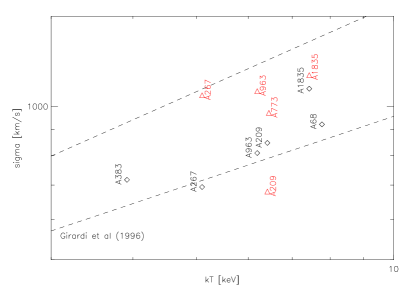
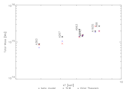
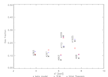
Fig. 1: Left: temperature-luminosity diagram as compared to the $90\%$ confidence level range from [Arnaud & Evrard, 1999] model. Right: temperature-velocity dispersion diagram as compared to the $90\%$ confidence level range from [Girardi et al., 1996] model (diamonds show values from [Bardeau & Kneib, 2003], triangles from [Dahle et al., 1990]).

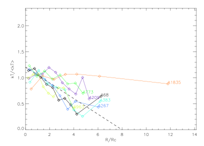
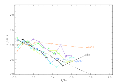
Fig. 2: Left: temperature-mass diagram, for different mass estimators, showing a mean power index of $1.576$. Right: gas mass fraction, for the same estimators, as a function of the X-ray temperature.

Fig. 3: Temperature profiles with radius rescaled either to core radius or virial radius units. The dashed line stands for the average slope in the central part of the polytropic simulation of [Loken et al., 2002].

We plotted a temperature-luminosity logarithmic diagram (Figure 3) for our subsample and compared it to the model proposed by [Arnaud & Evrard, 1999]. We observe that five clusters are indeed well co-aligned but following a shallower slope. A209 seems to depart from this alignment, as well as A1835 in a very significant manner. We also compared a temperature-velocity dispersion diagram with the model from [Girardi et al., 1996] and found it to be very close to the lower $90\%$ confidence level boundary, with again the exception of A1835.

Finally, the temperature-mass diagram is remarkably consistent with a mean power index of $1.576$, while the gas mass fraction seems to average about $10\%$ except again for A1835, as well as A209 and A773.

CONCLUSIONS & PERSPECTIVES

While early XMM-Newton observations ([Arnaud et al., 2001, Majerowicz et al., 2002]) did not confirm declining temperature profiles as seen by late ASCA observations ([Markevitch et al., 1998]) and Beppo-SAX ([DeGrandi & Molendi, 2002, Loken et al., 2002]), we find in the present analysis of 7 XBACS clusters that 6 of them do follow this kind of polytropic model. The seventh, A1835, systematically departs from the average in all diagrams (temperature-mass, temperature-luminosity), which confirms the rather complicated nature of its internal dynamics ([Majerowicz et al., 2002]).

However, we still are working toward the comparison of these emission weighted temperature profiles, that have been obtained without correction for PSF and may thus have been underestimated ([Markevitch, 2002]), with profiles built on the basis of hardness ratio maps, that may be adaptively handled to account for the PSF and binned between concentric isophotes rather than concentric annulii to adapt to non-spherical morphologies. Also, more work is intended so as to derive accurate error bars on each diagram, and attempt to estimate the virial radii from independent optical datasets.

Finally, this work has been made possible through the use of a pipeline analysis environment, specifically aimed at dealing with extended sources data from XMM-Newton instruments. It has confirmed the importance of maintenance and upgrades, to keep up-to-date with the instruments calibration database, as well as the need for such automatic tools in the purpose of building catalogs from the latest X-ray telescopes, so that massive cluster investigation may be possible in the future: access to large statistical samples, cross-compare mass and morphological measurements with optical data, correlate X-ray and Sunyaev-Zel’Dovich data…The ESA’s Planck satellite is promising thousands of millimetric clusters detections by the end of the decade, which could lead to narrower constraints on cosmology, provided an extensive X-rays database, like BAX ([Sadat et al., 2002]), also exists.

E-mail address of P.B. Marty: philippe.marty@ias.u-psud.fr

References

- [Abell, Corwin & Olowin, 1989] Abell, G.O., Corwin, H.G. & Olowin, R.P., 1989, ApJS, 70, 1
- [Allen, 1998] Allen, S.W., 1998, MNRAS, 296, 392
- [Arnaud & Evrard, 1999] Arnaud, M., & Evrard, A., 1999, MNRAS, 305, 631
- [Arnaud et al., 2001] Arnaud, M., et al., 2001, A&AL, 365, 80
- [Bahcall et al., 1997] Bahcall, N.A., et al., 1997, ApJL, 485, 53
- [Bardeau & Kneib, 2003] Bardeau, S., & Kneib, J.P., september 2002, private communication
- [Cavaliere & Fusco-Femiano, 1976] Cavaliere, A. & Fusco-Femiano, R., 1976, A&A, 49, 137
- [Czoske et al., 2001] Czoske, O., et al., 2001, A&A, 372, 391
- [Czoske et al., 2003] Czoske, O., et al., 2003, in preparation
- [Dahle et al., 1990] Dahle, H., et al., 2002, ApJS, 139, 313
- [DeGrandi & Molendi, 2002] De Grandi, S. & Molendi, S., 2002, ApJ, 567, 133
- [Dickey & Lockman, 1990] Dickey, J.M., & Lockman, F.J., 1990, ARAA, 28, 215
- [Ebeling et al., 1996] Ebeling, H., et al., 1996, MNRAS, 281, 799
- [Ebeling et al., 2000] Ebeling, H., et al., 2000, ApJ, 534, 133
- [Eke et al., 1996] Eke, V.R., et al., 1996, MNRAS, 282, 263
- [Evrard et al., 1996] Evrard, A., et al., 1996, ApJ, 469, 494
- [Girardi et al., 1996] Girardi, M., et al., 1996, ApJ, 457, 61
- [Loken et al., 2002] Loken, C., et al., 2002, ApJ, 579, 571
- [Lumb et al., 2002] Lumb, D. H., et al., 2002, A&A, 389, 93
- [Majerowicz et al., 2002] Majerowicz, S., et al., 2002, A&A, 394, 77
- [Markevitch et al., 1998] Markevitch, M., et al., 1998, ApJ, 503, 77
- [Markevitch, 2002] Markevitch, M., 2002, technical note (astro-ph/0205333)
- [Marty et al., 2002] Marty, P.B., et al., 2002, SPIE, 44851, 202 (astro-ph/0209270)
- [Marty et al., 2003] Marty, P.B., et al., 2003, submitted to A&A
- [Navarro, Frenk & White, 1997] Navarro, J.F., Frenk, C.S., & White, S.D.M., 1997, ApJ, 490, 493
- [Sadat et al., 2002] Sadat, R., Blanchard, A., & Mendiboure, C., 2002, ASR, ibid (astro-ph/0302171v2)
- [Smith et al., 2001] Smith, G.P., et al., I., 2001, ApJ, 552, 493
- [Smith et al., 2003] Smith, G.P., et al., 2003, ApJ, 590L, 79
- [Viana & Liddle, 1999] Viana, P.T.P. & Liddle, A.R., 1999, MNRAS, 303, 535