Star formation rate in galaxies from UV, IR, and H$\alpha$ estimators

Infrared (IR) luminosity of galaxies originating from dust thermal emission can be used as an indicator of the star formation rate (SFR). Inoue et al. (inoue00 (2000), IHK) have derived a formula for the conversion from dust IR luminosity to SFR by using the following three quantities: the fraction of Lyman continuum luminosity absorbed by gas ($f$), the fraction of UV luminosity absorbed by dust ($\epsilon$), and the fraction of dust heating from old ($\ga 10^{8}$ yr) stellar populations ($\eta$). We develop a method to estimate those three quantities based on the idea that the various way of SFR estimates from ultraviolet (UV) luminosity (2000 Å luminosity), H$\alpha$ luminosity, and dust IR luminosity should return the same SFR. After applying our method to samples of galaxies, the following results are obtained in our framework. First, our method is applied to a sample of star-forming galaxies, finding that $f\sim 0.6$, $\epsilon\sim 0.5$, and $\eta\sim 0.4$ as representative values. Next, we apply the method to a starburst sample, which shows larger extinction than the star-forming galaxy sample. With the aid of $f$, $\epsilon$, and $\eta$, we are able to estimate reliable SFRs from UV and/or IR luminosities. Moreover, the H$\alpha$ luminosity, if the H$\alpha$ extinction is corrected by using the Balmer decrement, is suitable for a statistical analysis of SFR, because the same correction factor for the Lyman continuum extinction (i.e., $1/f$) is applicable to both normal and starburst galaxies over all the range of SFR. The metallicity dependence of $f$ and $\epsilon$ is also tested: Only the latter proves to have a correlation with metallicity. As an extension of our result, the local ($z=0$) comoving density of SFR can be estimated with our dust extinction corrections. We show that all UV, H$\alpha$, and IR comoving luminosity densities at $z=0$ give a consistent SFR per comoving volume ($\sim 3\leavevmode\nobreak\ 10^{-2}h\leavevmode\nobreak\ M_{\odot}\leavevmode\nobreak\ {\rm yr}^{-1}\leavevmode\nobreak\ {\rm Mpc}^{-3}$). Useful formulae for SFR estimate are listed.

1 Introduction

During the history of the universe, galaxies have evolved forming stars. As a result, the present universe is filled with a large amount of stars and a significant amount of radiative energy originating from such stars. Therefore, tracing the star formation activity over all the history in the universe is fundamental to understand how the present universe has formed. To quantify the star formation activity, Star Formation Rate (SFR), defined as the stellar mass formed per unit time, is often estimated.

The star formation activity, more specifically the SFR, can be traced by young ($\mbox{age}\la 10^{7}$–$10^{8}$ yr) stars. Since short-lived massive stars are certain to be produced most recently, the SFR is traced with the luminosity of massive stars. One of the well known and commonly used tracers of massive stars is H$\alpha$ luminosity (e.g., Kennicutt kennicutt83 (1983)), because H$\alpha$ photons originate from the gas ionised by massive-star radiation. Since massive stars are the strong source for Ultra-Violet (UV) photons, UV luminosity is also used as an indicator of SFR. A general review for SFR indicators can be found in Kennicutt (1998a ).

In order to obtain a reliable estimate of the SFR, we have to take into account dust absorption (extinction) of UV and H$\alpha$ light. The H$\alpha$ luminosity (or more generally, the luminosity of hydrogen recombination lines) is decreased also by the extinction of Lyman continuum photons (e.g., Smith et al. smith78 (1978); Inoue et al. inouehk01 (2001); Inoue inoue01 (2001); Charlot & Fall charlot00 (2000); Charlot & Longhetti charlot01 (2001); Charlot et al. charlot02 (2002); Dopita et al. dopita03 (2003)). Quantifying the dust absorption is generally crucial in deriving the star formation history of a galaxy (e.g., Inoue et al. inoue01 (2001); Hopkins et al. hopkins01 (2001); Kewley et al. kewley02 (2002)) or of the universe (e.g., Flores et al. flores99 (1999); Steidel et al. steidel99 (1999); Meurer et al. meurer99 (1999)). Nevertheless, the correction for dust absorption usually requires an elaborate multi-wavelength or multi-band modelling (e.g., Calzetti calzetti01 (2001)).

There are some SFR indicators that are virtually free from dust extinction. One of them is the infrared (IR) luminosity originating from dust continuum emission (Kennicutt 1998a ). In this paper, we use the term IR to indicate the wavelength range where dust emission dominates the luminosity ($\sim 8$–1000 $\mu$m). We call the total luminosity of dust emission “dust IR luminosity.” Contrary to UV and H$\alpha$, dust IR luminosity traces the stellar radiation absorbed by dust. Thus, if a significant fraction of stellar radiation is absorbed by dust, detecting the dust IR emission is important. Recent ISO  (e.g., Takeuchi et al. takeuchi01 (2001)), COBE  (e.g., Hauser & Dwek hauser01 (2001)), and SCUBA observations (e.g., Blain et al. blain99 (1999); Barger et al. barger00 (2000)) have shown a significant contribution of dust IR emission to the total light in the universe over a large part of the cosmic history.

Theoretically the conversion factor between the dust IR luminosity and SFR is dependent on how efficiently stellar light is absorbed by dust and reprocessed in IR (e.g., Inoue et al. inoue00 (2000), hereafter IHK). In the analytic formula of IHK, the conversion factor between IR luminosity and SFR are described by using the following three parameters: $f$, $\epsilon$, and $\eta$, where $f$ is the fraction of Lyman continuum luminosity absorbed by hydrogen atoms, $\epsilon$ is the nonionising photons from young stars absorbed by dust, and $\eta$ is the fraction of IR luminosity originating from dust heating by old stars.

Let us note some remarks about the three parameters. IHK assume that the ionizing photons do not escape out of galaxies; that is, the fraction $1-f$ of the Lyman continuum luminosity is absorbed by dust grains. This can be justified for nearby galaxies, whose escape fraction of Lyman continuum photons is generally less than 10% (e.g., Leitherer et al. leitherer95 (1995); Deharveng et al. deharveng01 (2001)). For high-redshift (high-$z$) galaxies, it is still a matter of debate whether the escape fraction is high (Steidel et al. steidel01 (2001)) or low (Heckman et al. heckman01 (2001); Giallongo et al. giallongo02 (2002); Fernández-Soto et al. fernandez03 (2003)). We can regard $\epsilon$ as the fraction of UV (912–3650 Å) photons absorbed by dust, partly because almost all the radiative energy from young stars lies in the UV range, and partly because the dust absorption is much more efficient in UV than in optical (Buat & Xu buat96 (1996)). With respect to $\eta$, we should keep in mind that the definition of $\eta$ is temporal, not spatial as “cirrus”. Indeed, young stars can heat dust outside H ii regions and it is shown that the UV heating is also efficient in all the interstellar medium (ISM) via a diffuse interstellar radiation field not spatially associated with H ii regions (Buat & Xu buat96 (1996); Walterbos & Greenawalt walterbos96 (1996)). Our definition of $\eta$ is also different from the cool dust fraction as defined in Lonsdale Persson & Helou (lonsdale87 (1987)), because dust located out of H ii regions can be heated by UV radiation from massive stars and at the same time it can remain cool. Because of such a temporal definition of $\eta$, we have to specify the timescale on which the current SFR is traced (Section 2.1).

It is known that IR/UV flux ratio is a good indicator for the dust absorption in UV (Buat et al. buat99 (1999); Meurer et al. meurer99 (1999); Witt & Gordon witt00 (2000); Panuzzo et al. panuzzo03 (2003)). Therefore, UV and IR luminosities are useful not only to derive SFR but also to correct UV luminosity for dust absorption. By using H$\alpha$ luminosity in addition to UV and IR luminosities, we develop a method to estimate $f$, $\epsilon$, and $\eta$ (the principal quantities in the IHK formalism), and propose a way to obtain a reliable estimate of the SFR. Rosa-González et al. (rosa02 (2002)) also treat $\epsilon$ to estimate the SFR from dust IR luminosity, but we stress that $f$ and $\eta$ are also important (IHK). Charlot et al. (charlot02 (2002)) have compared the UV, IR, and H$\alpha$ SFR estimators based on a fully consistent model, which includes different extinctions between young and old stellar populations, non-Balmer emission lines, and various types of star formation histories (see also Charlot & Fall charlot00 (2000)). Charlot et al.  (charlot02 (2002)) also use [O ii] line luminosity (see also Gallagher et al. gallagher89 (1989)), which is not included in our paper, to estimate SFR This paper adopts a different approach: instead of modelling the details of radiative processes, we develop an independent and simple way to extract the important quantities for SFR estimates, so that our model might be applied easily to large data sets.

Hirashita et al. (hiro01 (2001), hereafter H01) suggest that those three quantities, $f$, $\epsilon$, and $\eta$, change as galaxies are enriched by metals. As a galaxy forms stars and recycles gas into ISM, the metallicity increases in some classes of models such as a closed-box model (e.g., Tinsley tinsley_sola80 (1980)). At the same time, dust grains are made from metals. In fact, metallicity is related to dust content (e.g., Issa et al. issa90 (1990); Schmidt & Boller schmidt93 (1993); Lisenfeld & Ferrara lisenfeld98 (1998); Dwek dwek98 (1998); Hirashita hiro99 (1999); Edmunds edmunds01 (2001)). H01 consider that the metallicity evolution results in the increase of dust optical depth. Consequently $f$ and $\epsilon$ (and possibly $\eta$) can be affected by metallicity evolution.

The aim of this paper is to develop a method to observationally estimate the quantities important for determining SFR. The luminosities in this paper are derived by assuming an isotropic radiation, which we expect to be reasonable in a statistical sense. First we reconstruct the IHK formula to make it consistent with our treatment in this paper (Section 2). In Section 3, then, we explain how to derive the important quantities ($f$, $\epsilon$, and $\eta$) for estimating SFR. In Section 4, we present the samples to which we apply our method. The statistical properties of various SFR indicators are discussed in Section 5, in which the metallicity dependence of $f$ and $\epsilon$ is also tested. In Section 6, we summarise our results and discuss possible application of our method to the cosmic Star Formation History (SFH) and to future survey data.

2 Reconstruction of SFR formulae

2.1 Reconsideration of the formula between $L_{\rm IR}$ and SFR

We reconstruct the conversion formula from dust IR luminosity ($L_{\rm IR}$) to SFR following the method of IHK. [In Dale et al. (dale01 (2001)), this luminosity is called “Total IR luminosity (TIR).”] A subset of the IRAS sample is commonly used to investigate the IR properties of galaxies, but the IRAS data are limited to the wavelength shorter than 120 $\mu$m. Therefore, the conversion formula from IRAS luminosity defined between 40 and 120 $\mu$m to the total dust IR luminosity is useful. We call the luminosity in the 40–120 $\mu$m range “FIR luminosity” ($L_{\rm FIR}$), whose way of estimate can be seen in Lonsdale Persson & Helou (lonsdale87 (1987)). Recently, data at longer wavelengths by ISO  have enabled Dale et al. (dale01 (2001)) to estimate the ratio $L_{\rm IR}/L_{\rm FIR}$ as a function of the IRAS 60 $\mu$m vs. 100 $\mu$m flux ratio. Hereafter we will use this their result unless otherwise stated. The ratio $L_{\rm IR}/L_{\rm FIR}$ is larger ($>2$) for normal star-forming galaxies (such as spiral galaxies) than for starburst galaxies. While the past analyses based on starburst models (e.g., Meurer et al. meurer99 (1999)) are not affected by a small difference between $L_{\rm IR}$ and $L_{\rm FIR}$ ($L_{\rm IR}/L_{\rm FIR}\simeq 1.4$; but see Calzetti et al. calzetti00 (2000), who derive $L_{\rm IR}/L_{\rm FIR}\simeq 1.8$), we have to be careful about the difference for normal galaxies.

The current star formation activity of galaxies can be traced by quantifying the amount of young stars. Thus, the term “young” should indicate the timescale on which the current star formation is traced. This timescale is denoted as $t_{\rm SF}$. For example, Inoue (2002a ) adopts $t_{\rm SF}\sim 10^{7}$ yr to trace the SFR. It is important to adopt a common timescale for all the SFR tracers. Since our aim is to work with monochromatic data near 2000 Å, the best choice of the timescale is that appropriate for this wavelength. We choose $t_{\rm SF}=10^{8}$ yr unless otherwise stated because the 2000 Å luminosity reaches its stationary value around $10^{8}$ yr in a constant SFR. Moreover, for large galaxies active in star formation but not necessarily starbursting, a constant SFR over $10^{8}$ yr seems reasonable since the strong correlation found between the H$\alpha$ and UV emissions (e.g., Buat et al. buat02 (2002), hereafter B02) argue for such a stationarity (but the stationarity for other samples is not necessarily supported; Sullivan et al. sullivan01 (2001)). Such a hypothesis strongly simplifies the analysis and helps the understanding. Since the duration of the current star formation activity may be shorter in starburst galaxies, we also examine $t_{\rm SF}=10^{7}$ yr in Section 5.2.

IHK have established a procedure to derive the conversion formula which connects dust IR luminosity and SFR. They start from the following relation among luminosities originating from young stars (Petrosian et al. petrosian72 (1972)):

$$L_{\rm IR}^{\rm SF}=L_{{\rm Ly}\alpha}+(1-f)L_{\rm Lyc}+\epsilon L_{\rm nonion}\,,$$ (1)

where $L_{\rm IR}^{\rm SF}$, $L_{{\rm Ly}\alpha}$, $L_{\rm Lyc}$, and $L_{\rm nonion}$ are various kinds of luminosities originating from young stars (luminosities of dust IR, Ly$\alpha$, Lyman continuum, and nonionising photons, respectively), and $f$ and $\epsilon$ are the fraction of Lyman continuum luminosity absorbed by gas and the fraction of nonionising photon luminosity absorbed by dust, respectively. In this formalism, all the Ly$\alpha$ photons are assumed to be absorbed by dust grains during some resonant scatterings. This assumption can be justified even for dust-deficient galaxies with 1% of the Galactic dust-to-gas ratio (H01), but we should be careful about this point if we apply our formula to objects from which a large amount of Ly$\alpha$ photons leak for some reason. As we mentioned in Section 1, it is also assumed that the Lyman continuum photons are absorbed either by gas or by dust and do not escape out of the galaxy.

All the three luminosities on the right-hand side in equation (1) are related to the bolometric luminosity of the young stars, $L_{\rm bol}^{\rm SF}$. In order to obtain such relations, we have run Starburst99 (Leitherer et al. leitherer99 (1999)) and made synthetic stellar spectra. We adopt the Salpeter stellar initial mass function (IMF) with the upper and lower masses of 100 $M_{\odot}$ and 0.1 $M_{\odot}$, respectively, constant SFR, and solar metallicity. We use the result at the age of $10^{8}$ yr, and this timescale should be equal to $t_{\rm SF}$. Then, we finally obtain $L_{\rm Lyc}=0.13L_{\rm bol}^{\rm SF}$ and $L_{\rm nonion}=0.87L_{\rm bol}^{\rm SF}$ from the synthetic spectrum at $t_{\rm SF}=10^{8}$ yr. In this paper, we adopt the same parameter set for the Starburst99 spectrum unless otherwise stated.

The Ly$\alpha$ luminosity is estimated under Case B (Osterbrock osterbrock89 (1989)) as (IHK)

$$L_{\rm Ly\alpha}=\frac{2}{3}N_{\rm Lyc}f^{\prime}h\nu_{\rm Ly\alpha}\,,$$ (2)

where $N_{\rm Lyc}$ is the number of ionising photons emitted per unit time, $h\nu_{\rm Ly\alpha}$ is the energy of a Ly$\alpha$ photon ($1.63\times 10^{-11}$ erg), and $f^{\prime}$ is the number fraction of Lyman continuum photons absorbed by gas (note that $f$ is the luminosity fraction of Lyman continuum absorbed by gas). Although the relation between $f$ and $f^{\prime}$ depends in a minor way on the extinction law for Lyman continuum photons and the shape of the Lyman continuum spectrum, $f\simeq f^{\prime}$ can be expected. There is a large difficulty in modelling the relation between $f$ and $f^{\prime}$ because of the lack of knowledge about the extinction law for the Lyman continuum photons. Thus, we simply adopt $f=f^{\prime}$ throughout this paper. By using the conversion from $N_{\rm Lyc}$ to $L_{\rm Lyc}$ predicted by the synthesised spectrum of the Starburst99 ($N_{\rm Lyc}=3.22\times 10^{10}L_{\rm Lyc}$ in the cgs units), we obtain $L_{\rm Ly\alpha}=0.34fL_{\rm Lyc}$. Then, equation (1) is reduced to

$$L_{\rm IR}^{\rm SF}=(0.13-0.085f+0.87\epsilon)L_{\rm bol}^{\rm SF}\,.$$ (3)

The Starburst99 result indicates that

$$\frac{\rm SFR}{M_{\odot}\leavevmode\nobreak\ {\rm yr}^{-1}}=1.79\times 10^{-10}\,\frac{L_{\rm bol}^{\rm SF}}{L_{\odot}}\,.$$ (4)

The dust IR luminosity, $L_{\rm IR}$, is the sum of two components originating from young ($<t_{\rm SF}$) stars and old ($>t_{\rm SF}$) stars (remember that $t_{\rm SF}=10^{8}$ yr unless otherwise stated). Then the fraction of old stellar contribution to $L_{\rm IR}$, $\eta$, is defined as

$$L_{\rm IR}^{\rm SF}=(1-\eta)L_{\rm IR}\,.$$ (5)

Considering the energy balance of dust, $\eta$ is also interpreted as the fraction of the energy input into dust (i.e., dust heating) from the old stellar population. Using equations (3), (4), and (5), we obtain

$$\frac{\rm SFR}{M_{\odot}\leavevmode\nobreak\ {\rm yr}^{-1}}=\frac{1.79\times 10^{-10}(1-\eta)}{0.13-0.085f+0.87\epsilon}\,\frac{L_{\rm IR}}{L_{\odot}}\,.$$ (6)

For the following convenience, we express the above conversion formula as

$${\rm SFR}=C_{\rm IR}(f,\,\epsilon,\,\eta)\,L_{\rm IR}\,,$$ (7)

that is, the conversion factor $C_{\rm IR}$ becomes

$$C_{\rm IR}(f,\,\epsilon,\,\eta)=\frac{1.79\times 10^{-10}(1-\eta)}{0.13-0.085f+0.87\epsilon}\leavevmode\nobreak\ [M_{\odot}\leavevmode\nobreak\ {\rm yr}^{-1}\leavevmode\nobreak\ L_{\odot}^{-1}]\,.$$ (8)

We observe that the conversion factor is determined by a set of $(f,\,\epsilon,\,\eta)$. We should note that this numerical expression for the conversion factor is based on the assumption that the star formation occurs at a constant rate for $10^{8}$ yr.

2.2 SFR from IR and UV emissions

We formally define SFR(IR) as

$${\rm SFR(IR)}=C_{\rm IR}^{\rm sb}\,L_{\rm IR}\,,$$ (9)

where we define the conversion factor, $C_{\rm IR}^{\rm sb}$, as follows:

$$C_{\rm IR}^{\rm sb} \equiv C_{\rm IR}(f=0,\,\epsilon=1,\,\eta=0)$$ (10)

$$= 1.79\times 10^{-10}\leavevmode\nobreak\ M_{\odot}\leavevmode\nobreak\ {\rm yr}^{-1}\leavevmode\nobreak\ L_{\odot}^{-1}\,.$$

If the radiation field in a galaxy is dominated by the young stars and all the radiation from stars is once absorbed by dust and reemitted in IR, SFR(IR) gives a reliable estimate for SFR (IHK). Indeed, $L_{\rm IR}=L_{\rm bol}^{\rm SF}$ in such a case, and equation (9) is the same as equation (4). This situation may be realised in starburst galaxies as assumed in Kennicutt (1998b ). Thus, we call the condition $(f,\,\epsilon,\,\eta)=(0,\,1,\,0)$ “dusty starburst approximation.” $C_{\rm IR}^{\rm sb}$ strongly depends on $t_{\rm SF}$ (Appendix A).

The intrinsic UV luminosity can be related to the SFR in a rather straightforward way. We adopt the 2000 Å monochromatic luminosity $L_{2000}$ to trace UV (B02), and we express the SFR formula as

$${\rm SFR(UV)}=C_{\rm 2000}\,L_{\rm 2000}\,,$$ (11)

where $C_{2000}$ can be calculated by using the Starburst99 spectrum (with the same parameters as above in Section 2.1) without dust absorption: $C_{2000}=2.03\times 10^{-40}\leavevmode\nobreak\ (M_{\odot}\leavevmode\nobreak\ {\rm yr}^{-1})/$(erg s^-1 Å^-1). The advantage of using 2000 Å monochromatic luminosity is that (i) 2000 Å is roughly the centre of the UV wavelength range (i.e., it traces the mean property of UV luminosity and extinction) and (ii) a large number of UV data are available at 2000 Å. If there is no dust absorption, SFR(UV) gives a reliable estimate of SFR.

Both SFR(IR) and SFR(UV) have their own disadvantages. If we know $\eta$, $(1-\eta)\,{\rm SFR(IR)}$ can be estimated from the observed $L_{\rm IR}$. However, $(1-\eta)\,{\rm SFR(IR)}$ would systematically underestimate the SFR, because a part of the stellar radiation is not absorbed by dust. This underestimate can be supplemented by SFR(UV) because most of the unabsorbed light from young stars is in UV. On the other hand, SFR(UV) can be formally estimated by multiplying the observed 2000 Å monochromatic luminosity with $C_{2000}$, but this always underestimates the SFR because an appreciable amount of the radiation from young stars is absorbed by dust and reprocessed into IR. This underestimate can be supplemented by $(1-\eta)\,{\rm SFR(IR)}$. Therefore, the following sum of UV and IR SFRs is expected to give a better approximation of the SFR:

$${\rm SFR}\simeq(1-\eta)\,{\rm SFR(IR)}+{\rm SFR(UV)}\,.$$ (12)

In the previous works such as Flores et al. (flores99 (1999)) and Buat et al. (buat99 (1999)), a simple sum ${\rm SFR(IR)}+{\rm SFR(UV)}$ has been adopted. This type of simple sum is examined in Section 5.5.

The formula for SFR(IR) (eq. 9) is derived by assuming that all the stellar light is absorbed by dust. On the other hand, the conversion to SFR(UV) (eq. 11) is made by assuming a theoretical stellar spectrum without extinction. Thus, we expect that equation (12) gives a reasonable estimate for the SFR if there is no dust absorption or if the dust optical depth against the stellar light is significantly larger than 1. In the case where there is some dust absorption, the shape of the absorbed spectrum in UV is modified by the differential absorption, and the IR light comes from only a part of the UV radiative energy. Therefore, it is not obvious whether or not equation (12) is valid for an arbitrary value of dust extinction (e.g., $E(B-V)$).

We check the validity of equation (12). We start from the Starburst99 spectrum. Here, we only consider the contribution from young stars (i.e., $\eta=0$), but we can apply the following consideration to $\eta>0$ by replacing SFR(IR) and $L_{\rm IR}$ with $(1-\eta)\,{\rm SFR(IR)}$ and $(1-\eta)\,L_{\rm IR}$, respectively. Assuming the Calzetti extinction curve (Calzetti et al. calzetti00 (2000)) for the dust absorption, we extinguish the synthesised stellar spectrum as a function of $E(B-V)$. The energy absorbed by dust is assumed to be equal to $L_{\rm IR}$. The energy absorbed by dust is estimated over all the range of the Starburst99 spectrum (100–1,600,000 Å) by using Calzetti et al.’s fitting formula. As a result, we obtain $L_{2000}$ (reduced according to the extinction) and $L_{\rm IR}$, and then SFR(IR) and SFR(UV) from equations (9) and (11), respectively. In this modelling, both SFR(IR) and SFR(UV) are proportional to SFR given in the Starburst99 calculation. Thus, we should examine if ${\rm[SFR(IR)+SFR(UV)]/SFR}=1$ is well satisfied. In Figure 1, we show SFR(IR)/SFR, SFR(UV)/SFR, and ${\rm[SFR(IR)+SFR(UV)]/SFR}$ as a function of $E(B-V)$ (dashed, dotted, and solid lines, respectively). The deviation of ${\rm[SFR(IR)+SFR(UV)]/SFR}$ from 1 is very small ($\la 6$%).

Figure 1: Star formation rates (SFRs) normalised with the true star formation rate. We show the part of the SFRs traced with UV and IR luminosities (dotted and dashed lines, respectively). The Calzetti extinction curve is assumed. The solid line shows the sum of the two SFRs and the correct SFR (normalised) should be 1. The small deviation of the solid line from 1 means that the sum of UV and IR SFRs traces the true SFR.

We have used the Calzetti curve because it is the only extinction curve derived from a sample of galaxies. But its validity is checked only for starburst galaxies. However, even if we adopt the Milky Way extinction curve (Cardelli et al. cardelli89 (1989); with $R_{V}=3.1$) instead of the Calzetti one, the difference of ${\rm[SFR(IR)+SFR(UV)]/SFR}$ from 1 is also $\la 7$%. Thus, we expect that the selection of a specific extinction curve does not change our conclusion that the sum of the IR and UV SFRs is an excellent indicator for the SFR.

It may be worth mentioning qualitatively the following details, whose quantitative discussion nevertheless depends on the assumed stellar spectrum and extinction curve. The slight overestimate of SFR for $E(B-V)\la 0.1$ is due to a smaller extinction (i.e., a larger escape fraction) of the 2000 Å light than that of the total UV light. Because of this, the 2000 Å monochromatic luminosity slightly overestimates the UV SFR. This point can be seen later in Figure 3 (Section 3.1). On the contrary, SFR(IR) tends to underestimate the SFR even in the high-extinction limit as we can see for $E(B-V)\ga 0.5$. This is because a small part of energy escapes from galaxies in optical and near-infrared wavelengths.

3 Estimates of the principal parameters

We explain how to determine the parameters $f$, $\epsilon$, and $\eta$, all of which appear in the IHK formula (eq. 6). We use the UV (2000 Å), H$\alpha$, and dust IR luminosities to derive those three quantities. We illustrate our procedures in Figure 2.

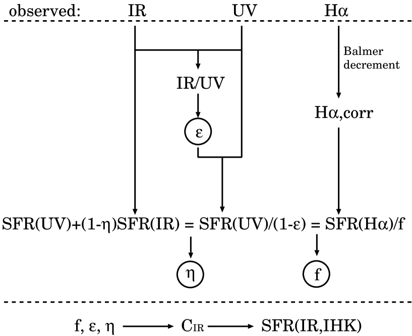
Figure 2: Summary of our method. We use three observational data (dust IR, UV, and H$\alpha$ luminosities) and derive three parameters $f$, $\epsilon$, and $\eta$, which are important for the conversion factor ($C_{\rm IR}$) from dust IR luminosity to star formation rate (SFR). The method is based on the consistency of the various SFRs derived from (1) the combination of UV and dust IR luminosities, (2) UV luminosity corrected for dust extinction, and (3) H$\alpha$ luminosity corrected for dust extinction. Finally, using the three parameters, we derive $C_{\rm IR}$, which gives another independent estimate for SFR (denoted as SFR(IR, IHK)).

3.1 $\epsilon$

The parameter $\epsilon$ is the fraction of UV photons absorbed by dust. Here, the UV wavelength range is defined between 912 Å and 3650 Å. The intrinsic UV luminosity is denoted as $L_{\rm UV}^{0}$. The observational UV luminosity $L_{\rm UV}$ can then be expressed as

$$L_{\rm UV}=(1-\epsilon)\,L_{\rm UV}^{0}\,.$$ (13)

Both $L_{\rm UV}$ and $L_{\rm UV}^{0}$ are defined as the luminosities in the UV wavelength range.

As mentioned in Section 2, we use the 2000 Å monochromatic luminosity to estimate the UV SFR. Therefore, we have to relate $\epsilon$ to $\epsilon_{2000}$ (defined as the fraction of 2000 Å monochromatic luminosity absorbed by dust). This relation depends on assumed models. One of the simplest ways to avoid such model dependence is to assume $\epsilon_{2000}=\epsilon$.

We quantify the uncertainty of this assumption $\epsilon_{2000}=\epsilon$. We adopt the Calzetti extinction curve to determine the absorbed fraction of UV light as a function of the extinction at 2000 Å. For a certain value of the 2000 Å extinction and the Starburst99 spectrum, we obtain the monochromatic luminosity after dust absorption for each wavelength. By integrating the monochromatic luminosity in all the UV wavelength range (912 – 3650 Å) and comparing this integration with the integration of the spectrum before dust absorption, we obtain the fraction of UV light absorbed by dust. Consequently, we obtain $\epsilon$ as a function of $\epsilon_{2000}$. The $\epsilon$ – $\epsilon_{2000}$ relation is plotted in Figure 3 (solid line). We find that $\epsilon_{2000}$ tends to underestimate $\epsilon$ but that the difference between the two is at most $\sim 0.06$. The difference in $\epsilon$ propagates to the estimates of $f$ and $\eta$ in our framework described later, causing the uncertainty of at most $\sim 20$% in those two parameters. However, we should keep in mind that the conversion from $\epsilon$ to $\epsilon_{2000}$ always has uncertainty if a specific model (i.e., a set of extinction curve and intrinsic spectrum) is selected. For example, if the Galactic extinction curve (Cardelli et al. 1989; with $R_{V}=3.1$) is assumed, we obtain the dashed line in Figure 3. In this case also, the difference from $\epsilon=\epsilon_{2000}$ is small enough. We prefer to avoid the model dependence by simply adopting $\epsilon_{2000}=\epsilon$.

Figure 3: Relation between $\epsilon$ (fraction of UV luminosity absorbed by dust) and $\epsilon_{2000}$ (fraction of 2000 Å monochromatic luminosity absorbed by dust) modelled for two types of extinction curves. The solid and dashed lines show the result for the Calzetti and Galactic extinction curves. The dotted line presents $\epsilon=\epsilon_{2000}$.

The IR/UV flux ratio can be used to estimate $\epsilon$ (Meurer et al. meurer99 (1999); Buat et al. buat99 (1999); B02). In principle, we can derive the extinction at 2000 Å from a reasonable model of the radiative transfer such as Xu & Buat (xu95 (1995)) if all the required data are available. Since the treatment of radiative transfer is beyond the scope of our simple analysis, we adopt a simplified relation between IR/UV ratio and 2000 Å extinction. For the SFG sample (see Section 4 for the sample description), we use the calibration of Buat et al. (buat99 (1999)) but expressed in $F_{\rm IR}/F_{2000}$ (dust IR vs. 2000 Å) flux ratio instead of $F_{\rm FIR}/F_{2000}$ (IRAS FIR vs. 2000 Å) one since the extrapolation of the total IR flux from that observed by IRAS has been made possible with the ISOPHOT observations (Dale et al. dale01 (2001)). We adopt the same definition of $F_{\lambda}$ ($\lambda$ is a wavelength in UV in units of Å) as that in Buat et al. (buat99 (1999)), i.e, $F_{\lambda}\equiv\lambda f_{\lambda}$, where $f_{\lambda}$ is the flux density per wavelength. Then we finally derive

$$A_{2000} \simeq 0.21+0.75\,\log(F_{\rm IR}/F_{2000})$$ (14)

$$+ 0.47[\log(F_{\rm IR}/F_{2000})]^{2}\,,$$

where $A_{2000}$ (mag) is the extinction at 2000 Å. We note that $F_{\rm IR}/F_{2000}=L_{\rm IR}/(\lambda_{2000}\,L_{\rm 2000})$, where $\lambda_{2000}=2000$ Å. This relation is derived from the energetics between IR and UV and is found rather insensitive to the details of the stellar spectrum if there is such an ongoing star formation activity as is seen in our samples (Buat & Xu buat96 (1996)). The fraction of 2000 Å light absorbed by dust can be related to $A_{2000}$ as

$$\epsilon=\epsilon_{2000}=1-10^{-A_{2000}/2.5}\,.$$ (15)

We also investigate starburst galaxies observed by IUE  as described in Section 4. For this IUE sample, we will use the extinction estimated by Calzetti et al. (calzetti00 (2000)). The extinction at 1600 Å can be observationally estimated for the IUE  sample as (Calzetti calzetti01 (2001))

$$A_{1600}\simeq 2.5\log\left[\frac{1}{1.68}\,\frac{F_{\rm IR}}{F_{1600}}+1\right]\,,$$ (16)

where $F_{1600}$ is defined in the same way as $F_{2000}$, i.e., the flux density at 1600 Å multiplied by 1600 Å. For nearby galaxies, $F_{1600}\simeq F_{2000}$ (Deharveng et al. deharveng94 (1994); Buat et al. buat99 (1999)), and thus we can use IR vs. 2000 Å luminosity ratio to estimate $F_{\rm IR}/F_{1600}$. Since $A_{2000}=0.9A_{1600}$ under the Calzetti extinction curve, $\epsilon_{2000}$, which is assumed to be equal to $\epsilon$, is estimated by

$$\epsilon=\epsilon_{2000}=1-10^{-0.9A_{1600}/2.5}\,.$$ (17)

3.2 $\eta$

We start from equation (12), where the basic idea is that the SFR measured with the IR emission is the SFR lost from the UV light because of the extinction. The left-hand side of equation (12) can be estimated by correcting the UV luminosity for dust absorption, i.e.,

$${\rm SFR}={\rm SFR(UV)}/(1-\epsilon)\,.$$ (18)

For the right-hand side of equation (12), SFR(IR) is estimated from $L_{\rm IR}$ (eq. 9) while SFR(UV) from $L_{2000}$ (eq. 11). Since $\epsilon$ is known after applying the method in Section 3.1, $\eta$ is determined from the following equation derived from equations (9), (11), (12) and (18):

$$(1-\eta)\,C_{\rm IR}^{\rm sb}\,L_{\rm IR}=\frac{\epsilon}{1-\epsilon}\,C_{2000}\,L_{2000}\,.$$ (19)

3.3 $f$

We start from the following relation between SFR and Lyman continuum luminosity:

$${\rm SFR}=C_{L_{\rm Lyc}}\,L_{\rm Lyc}\,,$$ (20)

where the Starburst99 spectrum indicates that $C_{L_{\rm Lyc}}=3.45\times 10^{-43}\leavevmode\nobreak\ (M_{\odot}\leavevmode\nobreak\ {\rm yr}^{-1})/({\rm erg\leavevmode\nobreak\ s}^{-1})$. We also obtain

$${\rm SFR}=C_{N_{\rm Lyc}}\,N_{\rm Lyc}\,,$$ (21)

where $N_{\rm Lyc}$ is the number of the ionising photons emitted per unit time, and $C_{N_{\rm Lyc}}=1.07\times 10^{-53}\leavevmode\nobreak\ (M_{\odot}\leavevmode\nobreak\ {\rm yr}^{-1})/{\rm s}^{-1}$ according to the Starburst99 spectrum.

Since the H$\alpha$ luminosity traces the amount of ionising photons, we connect the above expressions to the H$\alpha$ luminosity. According to Deharveng et al. (deharveng01 (2001)),

$$fN_{\rm Lyc}=7.34\times 10^{11}L_{\rm H\alpha}^{\rm c}\,,$$ (22)

where $L_{\rm H\alpha}^{\rm c}$ is the H$\alpha$ luminosity corrected for dust absorption by using the Balmer decrement (i.e., observed H$\alpha$ luminosity is multiplied by $10^{A({\rm H}\alpha)/2.5}$, where $A({\rm H}\alpha)$ (mag) is the extinction for the H$\alpha$ photons), and the quantities are expressed in the cgs units. This relation is determined from the Case B condition. Then we finally obtain the following relation from equations (21) and (22):

$${\rm SFR}=C_{\rm H\alpha}\,L_{\rm H\alpha}^{\rm c}/f\,,$$ (23)

where we obtain numerically $C_{\rm H\alpha}=7.34\leavevmode\nobreak\ 10^{11}\,C_{N_{\rm Lyc}}=7.89\leavevmode\nobreak\ 10^{-42}$ $(M_{\odot}\leavevmode\nobreak\ {\rm yr}^{-1})/({\rm erg\leavevmode\nobreak\ s}^{-1})$. The conversion factors $C_{L_{\rm Lyc}}$, $C_{N_{\rm Lyc}}$, and $C_{\rm H\alpha}$ are similar to the past estimates (e.g., Kennicutt 1998a ).

We estimate SFR in the left-hand side in equation (23) from UV luminosity, dust IR luminosity, and $\eta$ (known by the method in Section 3.2) by using equation (12). By using equations (9) and (11) in addition, $f$ is obtained:

$$f=\frac{C_{\rm H\alpha}\,L_{\rm H\alpha}^{\rm c}}{(1-\eta)\,C_{\rm IR}^{\rm sb}\,L_{\rm IR}+C_{2000}\,L_{2000}}\,.$$ (24)

4 Sample selection

One of the samples of nearby star-forming galaxies whose extinction properties and star formation rates are well examined is the SFG sample of B02. The sample consists of spiral and irregular galaxies located in clusters (Coma, Abell 1367, Cancer and Virgo). B02 also treat a starburst sample observed by IUE. We also use this sample (IUE  sample) in order to test the applicability of our method and to investigate the difference in properties. We adopt only the galaxies with a good measurement of Balmer decrement (i.e., with a direct measurement of the underlying stellar absorption). For the IUE sample, we only use the galaxies whose angular diameter is less than 1.5 arcmin in order to avoid the small aperture problem of IUE. The original quantities and the details are listed in Tables 1 and 2 of B02 for the SFG sample and the IUE  sample, respectively (see also the references therein).

The observational quantities used for our analysis are $L_{\rm H\alpha}^{\rm c}$ (the H$\alpha$ luminosity corrected for dust absorption by using the Balmer decrement), $L_{2000}$ (the monochromatic luminosity at 2000 Å), and $L_{\rm IR}$ (the dust IR luminosity). The dust IR luminosity is converted from the IRAS FIR luminosity by the method described in Dale et al. (dale01 (2001)). The three quantities for the SFG sample and the IUE sample are listed in Tables 1 and 2, respectively. We also examine the dependence on metallicity, which is traced with the oxygen abundance. The oxygen abundance is taken from Gavazzi et al. (2003, in preparation) for the SFG sample and from Calzetti et al. (calzetti94 (1994)) for the IUE sample. We call $12+\log{\rm(O/H)}$ metallicity in this paper. The solar metallicity corresponds to $12+\log{\rm(O/H)}=8.93$ (Anders & Grevesse anders89 (1989); Cox cox00 (2000)).

Table 1: SFG sample. The sample is taken from Buat et al. (2002).

Name	$L_{\rm 2000}$	$L_{\rm H\alpha}^{\rm c}$	$L_{\rm IR}$	$f$	$\epsilon$	$\eta$
	erg s-1 Å-1	erg s-1	erg s-1
VCC 25	8.91e+39	2.45e+41	6.76e+43	0.51	0.52	0.36
VCC 66	2.34e+39	1.12e+41	1.95e+43	0.84	0.54	0.36
VCC 89	7.94e+39	2.14e+41	7.08e+43	0.46	0.56	0.36
VCC 92	5.37e+39	2.69e+41	5.01e+43	0.83	0.57	0.37
VCC 131	1.02e+39	6.46e+39	4.17e+42	0.16	0.36	0.39
VCC 307	8.13e+39	7.24e+41	2.00e+44	0.80	0.77	0.41
VCC 318	2.04e+39	3.39e+40	4.79e+42	0.50	0.22	0.48
VCC 459	6.31e+38	1.41e+40	1.17e+42	0.73	0.16	0.55
VCC 664	8.51e+38	1.74e+40	2.24e+42	0.60	0.25	0.45
VCC 692	7.94e+38	1.32e+40	4.37e+42	0.36	0.44	0.37
VCC 801	2.40e+39	1.05e+41	3.02e+43	0.61	0.64	0.38
VCC 827	1.15e+39	3.31e+40	2.63e+43	0.27	0.76	0.40
VCC 836	1.29e+39	1.20e+41	3.89e+43	0.72	0.80	0.41
VCC 938	9.12e+38	3.16e+40	6.03e+42	0.69	0.49	0.36
VCC 1189	6.31e+38	1.00e+40	1.62e+42	0.47	0.24	0.46
VCC 1205	1.66e+39	2.19e+40	8.71e+42	0.29	0.43	0.37
VCC 1379	1.82e+39	2.57e+40	8.13e+42	0.34	0.39	0.38
VCC 1450	1.55e+39	2.40e+40	7.08e+42	0.36	0.39	0.38
VCC 1554	4.07e+39	2.24e+41	3.47e+43	0.96	0.55	0.36
VCC 1678	6.92e+38	1.29e+40	1.12e+42	0.63	0.13	0.61
CGCG 97087	3.72e+40	9.33e+41	2.14e+44	0.53	0.45	0.37
CGCG 100004	3.80e+39	1.55e+41	3.39e+43	0.69	0.56	0.36
CGCG 119029	3.16e+39	2.29e+41	5.75e+43	0.80	0.71	0.39
CGCG 119041	5.62e+38	8.13e+40	5.37e+43	0.43	0.92	0.44
CGCG 119043	1.48e+39	1.00e+41	3.63e+43	0.61	0.77	0.41
CGCG 119046	4.79e+39	2.19e+41	2.95e+43	0.94	0.47	0.36
CGCG 119047	3.55e+39	1.95e+41	7.76e+43	0.54	0.75	0.40
CGCG 119054a	1.86e+39	2.34e+41	2.04e+43	1.90	0.61	0.37
CGCG 119059	1.23e+39	4.37e+40	2.75e+43	0.34	0.75	0.40
CGCG 160055	1.26e+40	3.39e+41	1.91e+44	0.34	0.68	0.38
CGCG 160067	5.62e+39	3.09e+41	5.89e+43	0.85	0.60	0.37
CGCG 160139	1.02e+40	2.29e+41	4.17e+43	0.55	0.36	0.39
CGCG 160252	5.01e+39	3.80e+41	1.86e+44	0.50	0.83	0.42
Mean				0.57	0.53	0.40
$\sigma$				0.21	0.21	0.06

• This galaxy is not considered in taking the mean and $\sigma$ because $f$ is larger than 1.

Table 2: IUE starburst sample. The sample is compiled in Table 2 of Buat et al. (2002). We only list and use galaxies whose angular size is less than 1.5 arcmin in order to avoid the small aperture effect.

Name	$L_{\rm 2000}$	$L_{\rm H\alpha}^{\rm c}$	$L_{\rm IR}$	$f$	$\epsilon$	$\eta$
	erg s-1 Å-1	erg s-1	erg s-1
Mrk 499	8.51e+39	4.57e+41	2.00e+44	0.32	0.85	$-$0.03
Mrk 357	6.46e+40	2.09e+42	3.89e+44	0.50	0.60	$-$0.12
IC 1586a	4.37e+39	7.76e+41	8.71e+43	1.20	0.83	$-$0.05
Mrk 66	4.90e+39	1.02e+41	4.37e+43	0.25	0.69	$-$0.10
NGC 5860a	3.47e+39	1.05e+42	1.26e+44	1.27	0.89	$-$0.00
UGC 9560	6.17e+38	2.69e+40	2.82e+42	0.78	0.54	$-$0.13
NGC 6090	1.20e+40	3.80e+42	8.71e+44	0.74	0.94	0.05
IC 214	1.02e+40	1.15e+42	1.05e+45	0.20	0.96	0.08
Tol 1924$-$416	6.76e+39	2.75e+41	2.51e+43	0.81	0.49	$-$0.14
Haro 15	1.38e+40	3.02e+41	1.23e+44	0.26	0.69	$-$0.10
NGC 6052	5.50e+39	3.89e+41	2.75e+44	0.23	0.92	0.02
NGC 3125	5.62e+38	3.89e+40	7.59e+42	0.63	0.77	$-$0.07
NGC 1510	2.34e+38	5.50e+39	1.23e+42	0.39	0.57	$-$0.12
NGC 1614	3.98e+39	5.62e+42	1.78e+45	0.67	0.99	0.20
NGC 7673	5.01e+39	4.37e+41	1.17e+44	0.52	0.85	$-$0.03
NGC 7250	8.71e+38	2.88e+40	1.07e+43	0.32	0.75	$-$0.08
NGC 5996	1.38e+39	1.74e+41	5.37e+43	0.50	0.90	0.00
NGC 1140	1.70e+39	9.33e+40	1.62e+43	0.63	0.70	$-$0.09
NGC 4194a	2.40e+39	1.91e+42	3.39e+44	1.04	0.97	0.11
Mean				0.48	0.76	$-0.04$
$\sigma$				0.20	0.15	0.09

• Those galaxies are not considered in taking the mean and $\sigma$ because $f$ is larger than 1.

From the arguments on dust temperature and equivalent widths of the Balmer lines, B02 show that the IUE  sample consists of galaxies with higher star formation activity than the SFG sample. The IUE  sample can be regarded as a class of “starburst” galaxies, while the SFG sample can be representative of “normal” star-forming galaxies (spiral galaxies and irregular galaxies). We use the term “normal” and “starburst” to indicate a rough classification of star formation activity in this paper, and those two classes are often identified with the SFG sample and the IUE  sample, respectively.

5 Results

In this section, we first apply our method to the SFG sample (Section 5.1), because the IUE  sample may still have an effect of the small aperture even after we put the criterion for the angular size. The robustness of the method against the model is also examined for the SFG sample (Section 5.2). Then, we apply our method to the IUE  sample in Section 5.3. The SFRs derived from the IHK method is compared with the best-estimate SFR in order to test the validity of the IHK formula (Section 5.4). Other SFR estimators are also examined in Section 5.5. The metallicity dependence of some of the quantities ($f$ and $\epsilon$) is investigated in Section 5.6 in order to test the hypothesis in H01. The luminosities and the SFR conversion factors are summarised in Table 3.

Table 3: Luminosities and SFR conversion factors on the timescale of $t_{\rm SF}=10^{8}$ yr.

Quantity	Value	Units	Definition / comment
$L_{2000}$		erg s-1 Å-1	2000 Åmonochromatic
$L_{\rm H\alpha}^{\rm c}$		erg s-1	corrected for Balmer decrement
$L_{\rm IR}$		erg s-1	dust IRa
$C_{2000}$	$2.03\times 10^{-40}$ b	$(M_{\odot}\leavevmode\nobreak\ {\rm yr}^{-1})$/(erg s-1 Å-1)	to be divided by $(1-\epsilon)$
$C_{\rm H\alpha}$	$7.89\times 10^{-42}$ c	$(M_{\odot}\leavevmode\nobreak\ {\rm yr}^{-1})$/(erg s-1)	to be divided by $f$
$C_{\rm IR}^{\rm sb}$	$1.79\times 10^{-10}$ d	$M_{\odot}\leavevmode\nobreak\ {\rm yr}^{-1}\leavevmode\nobreak\ L_{\odot}^{-1}$	dusty starburst approximation for IR
$C_{\rm IR}$	equation (8)	$M_{\odot}\leavevmode\nobreak\ {\rm yr}^{-1}\leavevmode\nobreak\ L_{\odot}^{-1}$	$f$, $\epsilon$, and $\eta$ are necessary

• The total luminosity of dust emission derived from the IRAS luminosity correcting for the contribution from longer ($\lambda>120\leavevmode\nobreak\ \mu$m) wavelengths. Dale et al. (dale01 (2001)) is used for the correction, but the difference between correction models is well less than 30% (e.g., the difference from Nagata et al. nagata02 (2002)).

• If $t_{\rm SF}=10^{7}$ yr, the value becomes $3.18\times 10^{-40}$.

• The value is unchanged for $t_{\rm SF}=10^{7}$ yr.

• If $t_{\rm SF}=10^{7}$ yr, the value becomes $2.72\times 10^{-10}$.

5.1 $f$, $\epsilon$, and $\eta$ for the SFG sample

One of the characteristics of the SFG sample is that the H$\alpha$ (corrected for dust absorption by the Balmer decrement) to UV flux ratio is lower than that expected for $f=1$ under a constant SFR over $10^{8}$ yr (B02). This may indicate that some significant fraction of ionising photons is absorbed by dust grains. Inoue (inoue01 (2001)), after analysing the individual H ii regions of some Local Group galaxies, also reaches the same conclusion. Charlot et al. (charlot02 (2002)) also concluded the same thing from their analysis of the Stromlo-APM redshift survey data. Thus, we expect to find a fraction $f$ significantly lower than 1.

In Table 1, we list $f$, $\epsilon$, and $\eta$ for each galaxy. By definition, $f$ should be between 0 and 1, but only CGCG 119054 shows $f$ significantly larger than 1. We consider this to be due to the overcorrection of H$\alpha$ absorption. Indeed, $A({\rm H}\alpha)=2.47$ mag is the largest of all the SFG sample and the correction of dust absorption is as large as a factor of 9.7. With such a large extinction, the extinguished H$\beta$ flux measurement could be very uncertain. As a result, the extinction derived from the Balmer decrement measurement could have a significant uncertainty. Therefore, we omit CGCG 119054 in the following analysis.

The mean values and the standard deviations ($\sigma$) of $f$, $\epsilon$, and $\eta$ are shown at the bottom of Table 1. We calculated those values excluding CGCG 119054. As expected at the beginning of this subsection, $f$ is significantly smaller than 1. The mean value of $f$ (0.57) indicates that about 40% of the ionising photons are directly absorbed by dust grains before being processed into recombination lines. This can be a reason for the systematic underestimate of H$\alpha$ SFR relative to SFRs from other indicators (e.g., Cram et al. cram98 (1998); B02). We also observe from the mean of $\epsilon$ (0.53) that the half of the UV is absorbed by dust and reprocessed into IR. If we convert $\epsilon=0.53\pm 0.21$ into $A_{2000}$ by using equation (15) and assuming $\epsilon=\epsilon_{2000}$ (i.e., by $A_{2000}=-2.5\log(1-\epsilon)$), we obtain $A_{2000}=0.82^{+0.64}_{-0.40}$. This confirms the result of B02. The value of $\eta\sim 0.4$ indicates that about 40% of the dust heating is due to old (age $>t_{\rm SF}=10^{8}$ yr) stars, which have nothing to do with the current SFR. Misiriotis et al. (misiriotis01 (2001)) also find the contribution of old stellar populations to grain heating to be $\sim 40$% for a sample of spiral galaxies.

We also show the relations among the three quantities in Figure 4. We see that there is no evidence for correlation either between $f$ and $\epsilon$ ($r=0.055$; $r$ is the correlation coefficient) or between $f$ and $\eta$ ($r=-0.017$). There seems to be a tight relation between $\eta$ and $\epsilon$, but this tightness results from our formulation that determines both $\eta$ and $\epsilon$ as a function of IR/UV flux ratio (see Sections 3.1 and 3.2). In reality, there is a scatter in the relation between $\epsilon$ and IR/UV flux ratio (see Fig. 1 of Buat et al. buat99 (1999)). This scatter also disperse the $\eta$–$\epsilon$ relation and the standard deviation of $\eta$ would increase significantly. However, the mean values of $\eta$ should still be $\sim 0.4$.

Figure 4: Diagrams of (a) $f$ vs. $\epsilon$, (b) $f$ vs. $\eta$, and (c) $\eta$ vs. $\epsilon$ for the SFG sample, where $f$ is the fraction of ionising radiation absorbed by gas, $\epsilon$ is the fraction of UV luminosity absorbed by dust, and $\eta$ is the fraction of dust heating by the old ($>10^{8}$ yr) stellar population.

5.2 Model uncertainty

We examine how much the three quantities ($f$, $\epsilon$, and $\eta$) are changed by the uncertainty in model assumptions. One of the sources for the uncertainty is the conversion between the IRAS FIR luminosity to the (total) dust IR luminosity. We have used Dale et al. (dale01 (2001)) for this conversion. If we adopt Nagata et al. (dale02 (2002)) for this conversion (their FIR2 is used), the mean values of $f$, $\epsilon$, and $\eta$ change to 0.62, 0.50, and 0.39, respectively (the standard deviations being 0.24, 0.20, and 0.06, respectively). The difference in $L_{\rm IR}/L_{\rm FIR}$ between Dale & Helou (dale02 (2002)) and Dale et al. (dale02 (2002)) is smaller than that between Nagata et al. (nagata02 (2002)) and Dale et al. (dale01 (2001)). Therefore, with the available $L_{\rm IR}/L_{\rm FIR}$ models, the parameters are determined within an uncertainty of $\sim 10$%.

Rosa-González et al. (rosa02 (2002)) also calculated $\epsilon$. Some of their galaxies (13 galaxies) overlap with our IUE  sample, whose $\epsilon$ is derived later (Section 5.3; Table 2). They determined $\epsilon$ in a similar manner as ours, but not the same (e.g., the way of the estimate of IR/UV flux ratio is different). The agreement between our $\epsilon$ and theirs is extremely good (the difference is within 0.05 except for Mrk 66, for which we obtain $\epsilon=0.69$ while they derive $\epsilon=0.58$). This supports the robustness of $\epsilon$ for the IUE  sample. For the SFG sample, the literature that analysed $\epsilon$ is not found, and we cannot argue that other models support our derivation of $\epsilon$.

We should remember that the conversion factors between SFR and various luminosities depend on age, or more generally on SFH (e.g., Sullivan et al. sullivan01 (2001)). In particular, the relative luminosity ratio between UV and Lyman continuum (or recombination lines) is sensitive to age. In a constant SFR, the luminosity of the Lyman continuum reaches its stationary value at the age of $\sim 10^{7}$ yr, while the UV luminosity becomes stationary at $\sim 10^{8}$ yr. In the above, we have adopted $t_{\rm SF}=10^{8}$ yr for the age, but we could adopt $t_{\rm SF}=10^{7}$ yr to have an idea how much the quantities change in response to the SFH. Some of the conversion factors at $10^{7}$ yr change: $C_{2000}$, $C_{\rm IR}$, and $C_{\rm IR}^{\rm sb}$ take the values described in Appendix A, while $C_{L_{\rm Lyc}}$, $C_{N_{\rm Lyc}}$, and $C_{\rm H\alpha}$ are the same as those at $10^{8}$ yr.

In the framework of Starburst99, it is very difficult to have a spectrum for an arbitrary SFH, but it is easy and computationally economical to change only the age under a constant SFH. Thus, we only change the age here. By using another population synthesis code, we have also tested the difference between a constant SFR and an exponentially decaying SFR. As long as the exponential decaying timescale is comparable to (or longer than) the duration of the star formation ($t_{\rm SF}$), the change of th results is not so drastic as the difference between $t_{\rm SF}=10^{8}$ yr and $t_{\rm SF}=10^{7}$ yr. If a galaxy has a decaying timescale much shorter than $t_{\rm SF}$, it would not be classified with a star-forming galaxy and would not included in our sample.

If those coefficients for $t_{\rm SF}=10^{7}$ yr are adopted, we obtain the mean values $f=0.39$, $\epsilon=0.53$, and $\eta=0.38$ (the standard deviations, $\sigma$, being 0.20, 0.21, and 0.06, respectively). It is natural that $\epsilon$ does not change at all because it is determined from IR/UV ratio, which is independent of the conversion factors. While $\eta$ is not sensitive to the conversion factors, $f$ changes significantly depending on the assumed $t_{\rm SF}$. Recalling that $f$ is determined from the ratio between the SFR traced with H$\alpha$ and the SFR traced with UV and IR, the sensitive change of $f$ against $t_{\rm SF}$ comes from the difference in the conversion factors for the UV and IR SFRs. Therefore, the typical age of the current star-forming activity is important if the age is shorter than $10^{8}$ yr. We expect that our SFG sample has a continuous mode of the star formation because the correlation between H$\alpha$ and UV luminosities is good (B02). However, for a starburst sample such as the IUE  sample, the duration of the present starburst could be shorter than $10^{8}$ yr. Calzetti et al. (calzetti94 (1994)) assumed a constant SFR over 2 $10^{7}$ yr for these galaxies. The correlation between H$\alpha$ and UV luminosities is not so good as that for the SFG galaxies (B02), which also suggests that the sample has a diverse property in SFH on a timescale shorter than $10^{8}$ yr. However, since we do not know the typical age of those sample, we adopt $t_{\rm SF}=10^{8}$ yr also for this sample. If $t_{\rm SF}$ is shorter than $10^{8}$ yr, $f$ becomes smaller. Some mechanisms are proposed for a short-term variation of SFR on a galactic scale (Kamaya & Takeuchi kamaya97 (1997) and references therein).

The spectral synthesis model used to derive the conversion factors is another source of uncertainty. We have seen above that the relative values between $C_{\rm H\alpha}$ and $C_{2000}$ (or $C_{\rm IR}$) is the largest source for the uncertainty in $f$, although $\eta$ is determined quite robustly. Based on pegase synthesis code (Fioc & Rocca-Volmerange fioc97 (1997)), for example, the construction of the conversion factors are possible. Two of the conversion factors ($C_{\rm H\alpha}$ and $C_{2000}$ in our notation) are thus obtained by Sullivan et al. (sullivan01 (2001)) for various age and metallicity. However, both of their $C_{2000}$ and $C_{\rm H\alpha}$ are similar to ours (difference is $<20$%). Therefore, the difference in $f$ between the two synthesis codes is small and the difference in $t_{\rm SF}$ causes larger difference in $f$. The difference in metallicity affects $C_{\rm H\alpha}$ as largely as that in $t_{\rm SF}$, but the solar metallicity well approximates the metallicity of our samples. As long as the metallicity is between 1/10 and 3 solar metallicity, the major source for the uncertainty is the age, not the metallicity.

5.3 Application to the IUE sample

The IUE sample is also analysed in the way described in Section 5.1. If we adopt the conversion factors for $t_{\rm SF}=10^{8}$ yr, we obtain the results as listed in Table 2. For some of the galaxies, $f$ is larger than 1, although $f<1$ by definition. We suspect that this is due to the same reason as CGCG 119054 (Section 5.1). Indeed, the galaxies whose $f$ is larger than 1 have a large $A({\rm H}\alpha)$ (1.42, 1.69, and 1.96 for IC 1586, NGC 5860, and NGC 4194, respectively). We exclude those galaxies from the following analysis. The mean values ($\pm\sigma$) are $f=0.48$ ($\pm 0.20$), $\epsilon=0.76$ ($\pm 0.15$), and $\eta=-0.04$ ($\pm 0.09$). If we apply the conversion factors at $10^{7}$ yr (i.e., we adopt $t_{\rm SF}=10^{7}$ yr), we obtain $f=0.30$ ($\pm 0.13$), $\epsilon=0.76$ ($\pm 0.15$), and $\eta=-0.07$ ($\pm 0.09$). As seen in the SFG sample, $f$ is sensitive to $t_{\rm SF}$ also for the IUE  sample.

The extinctions for Lyman continuum and UV are both larger for the IUE  sample than for the SFG sample. For the IUE  sample, about 50% of the Lyman continuum photons and roughly 80% of the UV photons are absorbed by dust grains. Moreover almost all the dust heating source is the stellar population younger than $10^{8}$ yr for the IUE  sample, since $\eta\sim 0$. This is consistent with the starburst property of the IUE  sample, whose current star formation activity dominates the luminosity of galaxies.

We examine the correlation between the quantities. There is no evidence for the correlations between $f$ and $\epsilon$ ($r=-0.12$) and between $f$ and $\eta$ ($=-0.04$). There seems to be a tight relation between $\epsilon$ and $\eta$, but this results from the same reason as the SFG sample (Section 5.1). In reality, the scatter should be much larger if we consider the scatter in the relation between IR/UV flux ratio and $\epsilon$.

5.4 Validity of IHK

One of our main aims is to examine the conversion formula of IHK (eq. 7). In order to see if the IHK formula works well or not, we should know the best estimate for the SFR first of all. We have shown that the SFR is traced very well by using IR and UV SFRs as equation (12). Therefore, in this paper the real SFR estimated observationally is defined as

$${\rm SFR(best)}\equiv(1-\eta)\,C_{\rm IR}^{\rm sb}\,L_{\rm IR}+C_{2000}\,L_{2000}\,\,.$$ (25)

Since $f$, $\eta$ and $\epsilon$ are supposed to be known at this step, we can examine the conversion factor for the IR SFR by using the IHK method. We define the following SFR(IR, IHK) by using the IHK conversion factor (eq. 8):

$${\rm SFR(IR,\,IHK)}\equiv C_{\rm IR}(f,\,\epsilon,\,\eta)\,L_{\rm IR}\,.$$ (26)

Using the quantities $(f,\,\epsilon,\,\eta)$ derived for each galaxy in Table 1, we show the relation between SFR(IR, IHK) and SFR(best) in Figure 5. We find that SFR(IR, IHK) agrees with SFR(best) within a difference of $\sim 30$% (for 70% of the SFG sample, the difference is within 10%). Therefore, if we know the three quantities, the IHK method approximates the SFR very well.

Figure 5: Star formation rate derived from the IHK method, SFR(IR, IHK), compared with the best-estimate SFR for the SFG sample and the IUE  sample (a and b, respectively).

For a general sample, we do not necessarily have all the three (UV, H$\alpha$, and dust IR) luminosities. In this case, $C_{\rm IR}(f,\,\epsilon,\,\eta)$ cannot be obtained by our method. Thus, in the next subsection, we examine various SFRs derived from a limited number of luminosities.

5.5 SFR

Here we investigate SFRs derived from various indicators. In Figures 6a–d, we compare SFR(UV), SFR(IR), SFR(IR, UV), and SFR(H$\alpha$) with SFR(best) for the SFG sample. Figure 6a clearly shows that SFR(UV) underestimates the SFR because of dust absorption. The ratio SFR(UV)/SFR(best) is equal to $(1-\epsilon)$ (eq. 18). If we can estimate $\epsilon$ (UV extinction) for each galaxy, SFR(UV)/$(1-\epsilon)$ gives the best estimate of SFR.

Figure 6: Various SFRs of the SFG sample plotted against the best-estimate SFR. The solid lines show the equality of the two SFRs plotted in each figure. (a) SFR(UV) (without any extinction correction). The dotted and dashed lines indicate the “extinction-corrected” relations, SFR(UV)/$(1-\epsilon)={\rm SFR(best)}$ with $\epsilon=0.53$ (the mean of the SFG sample) and with $\epsilon=0.76$ (the mean of the IUE  sample), respectively. (b) SFR(IR) converted directly from the dust IR luminosity by multiplying $C_{\rm IR}^{\rm sb}$. The solid line shows ${\rm SFR(IR)}={\rm SFR(best)}$. The dotted and dashed lines present the trend for the SFG sample and the IUE  sample, respectively. (c) ${\rm SFR(IR,\,UV)}\equiv{\rm SFR(UV)}+{\rm SFR(IR)}$. (d) SFR(H$\alpha$) derived from the H$\alpha$ luminosity corrected for the Balmer decrement. The dotted and dashed lines show the relations corrected for the Lyman continuum extinction with $f=0.57$ (the mean of the SFG sample) and $f=0.48$ (the mean of the IUE  sample, respectively.

The discrepancy between SFR(UV) and SFR(best) tends to be small for small SFR. For ${\rm SFR(best)}\la 1\leavevmode\nobreak\ M_{\odot}\leavevmode\nobreak\ {\rm yr}^{-1}$, SFR(UV) gives a good estimate for the real SFR (see also Bell & Kennicutt bell01 (2001)). This means that there is a positive correlation between SFR and $\epsilon$ as pointed out also by Hopkins et al. (hopkins01 (2001)). This correlation may only reflect the size effect, since a large galaxy may tend to contain a lot of star-forming regions and at the same time a large optical depth of dust (Wang & Heckman wang96 (1996); Buat & Burgarella buat98 (1998)).

We expect that ${\rm SFR(UV)}/(1-\epsilon)$ with $\epsilon=0.53$ gives a better estimate for the SFR. The dotted line in Figure 6a shows the relation ${\rm SFR(UV)}/(1-\epsilon)={\rm SFR(best)}$ with $\epsilon=0.53$. We observe that ${\rm SFR(UV)}/(1-\epsilon)$ with $\epsilon=0.53$ systematically overestimates the SFR for ${\rm SFR}\la 1\leavevmode\nobreak\ M_{\odot}\leavevmode\nobreak\ {\rm yr}^{-1}$, because the data points lie in the region ${\rm SFR(UV)}/(1-\epsilon)>{\rm SFR(best)}$. Thus, the dust correction should be varied depending on the SFR. Because of a large variety in $\epsilon$, the scatter of SFR(UV) is larger than that of any other estimators. The dashed line in Figure 6 represents the relation applied to the IUE  sample (i.e., $\epsilon=0.76$).

Figure 6b indicates that SFR(IR) estimates the SFR quite well for ${\rm SFR}\ga 1\leavevmode\nobreak\ M_{\odot}\leavevmode\nobreak\ {\rm yr}^{-1}$. However, we should keep in mind that this is the result of the cancellation of the following under- and overestimate (Kennicutt 1998a ; Inoue 2002a ): SFR(IR) overestimates the SFR by a factor $1/(1-\eta)$ because a part of the IR dust luminosity originates from the old stellar population; SFR(IR) underestimates the SFR because a part of the radiation originating from young stars is not absorbed by dust, and thus is not traced by IR. However, SFR(IR) systematically underestimates SFR(best) when the SFR is lower than 1 $M_{\odot}\leavevmode\nobreak\ {\rm yr}^{-1}$, because the major part of the energy is radiated in UV. Accordingly, SFR(UV) provides a reasonable estimate of SFR for ${\rm SFR}\la 1\leavevmode\nobreak\ M_{\odot}\leavevmode\nobreak\ {\rm yr}^{-1}$.

The conversion factor for the IR luminosity can be tested by using the IHK conversion factor $C_{\rm IR}(f,\,\epsilon,\,\eta)$. In treating a sample of galaxies, a typical values of $f$, $\epsilon$, and $\eta$, for example the mean values ($f=0.57$, $\epsilon=0.53$, and $\eta=0.40$ for the SFG sample), are useful. If we put those mean values, we find that $C_{\rm IR}=2.0\times 10^{-10}\leavevmode\nobreak\ M_{\odot}\leavevmode\nobreak\ {\rm yr}^{-1}\leavevmode\nobreak\ L_{\odot}^{-1}$. This value is similar to $C_{\rm IR}^{\rm sb}=1.79\times 10^{-10}\leavevmode\nobreak\ M_{\odot}\leavevmode\nobreak\ {\rm yr}^{-1}\leavevmode\nobreak\ L_{\odot}^{-1}$. If we use $2.0\times 10^{-10}\leavevmode\nobreak\ M_{\odot}\leavevmode\nobreak\ {\rm yr}^{-1}\leavevmode\nobreak\ L_{\odot}^{-1}$ instead of $C_{\rm IR}^{\rm sb}$ to estimate SFR(IR), the data points in Figure 6b shift upwards. In order not to complicate the figure, we shift the solid line down to the dotted line. The dashed line shows the same thing for $C_{\rm IR}=2.4\times 10^{-10}\leavevmode\nobreak\ M_{\odot}\leavevmode\nobreak\ {\rm yr}^{-1}\leavevmode\nobreak\ L_{\odot}^{-1}$, which is representative for the IUE  sample (Table 4). If $f$, $\epsilon$, and $\eta$ move their 1 $\sigma$ ranges, $C_{\rm IR}=1.3$ – $3.5\times 10^{-10}\leavevmode\nobreak\ M_{\odot}\leavevmode\nobreak\ {\rm yr}^{-1}\leavevmode\nobreak\ L_{\odot}^{-1}$. For a comparison, we should note that Buat & Xu (buat96 (1996)) derive a similar range $C_{\rm IR}=0.79$ – $2.6\times 10^{-10}\leavevmode\nobreak\ M_{\odot}\leavevmode\nobreak\ {\rm yr}^{-1}\leavevmode\nobreak\ L_{\odot}^{-1}$, where we assume $L_{\rm IR}/L_{\rm FIR}=2.4$ (the mean for the SFG sample).

Table 4: Recommended conversion factors from each luminosity to SFR on the timescale of $t_{\rm SF}=10^{8}$ yr.

Luminositya	Multiplying factorb		Comment
	normalc	starburstd
$L_{2000}$	$4.3\times 10^{-40}$	$8.5\times 10^{-40}$	large dispersion in extinction
			systematic underestimate for $\la 1\leavevmode\nobreak\ M_{\odot}\leavevmode\nobreak\ {\rm yr}^{-1}$
$L_{\rm H\alpha}^{\rm c}$	$1.4\times 10^{-41}$	$1.6\times 10^{-41}$	similar factor for both (“universal”)
			applicable to any SFR
$L_{\rm IR}$	$2.0\times 10^{-10}$	$2.4\times 10^{-10}$	risk of underestimate for $\la 1\leavevmode\nobreak\ M_{\odot}\leavevmode\nobreak\ {\rm yr}^{-1}$
Other formulae
$(1-\eta)\,C_{\rm IR}^{\rm sb}\,L_{\rm IR}+C_{2000}\,L_{2000}$			$\eta$ necessary
$C_{\rm IR}^{\rm sb}\,L_{\rm IR}+C_{2000}\,L_{2000}$			systematic overestimate for normal galaxies

• $L_{\rm H\alpha}^{\rm c}$ is the H$\alpha$ luminosity after the correction for the H$\alpha$ extinction ($A({\rm H}\alpha)$). $L_{\rm IR}$ is the total luminosity of dust emission derived from IRAS  40–120 $\mu$m luminosity and 60 $\mu$m vs. 100 $\mu$m flux ratio (Dale et al. dale01 (2001)).

• The units are the same as in Table 3.

• The SFG sample is assumed to be representative of normal star-forming galaxies.

• The IUE  sample is assumed to be representative of starburst galaxies.

We also examine the following SFR defined as a simple sum of IR and UV SFRs:

$${\rm SFR(IR,\,UV)}\equiv C_{\rm IR}^{\rm sb}\,L_{\rm IR}+C_{2000}\,L_{2000}\,.$$ (27)

This kind of sum is adopted in Flores et al. (flores99 (1999)) and Buat et al. (buat99 (1999)). In Figure 6c, we show the relation between SFR(IR, UV) and SFR(best). We observe that SFR(IR, UV) overestimates the SFR because the fraction $\eta$ related to the old stars is not subtracted from $L_{\rm IR}$. However, the overestimate is not so large, $\sim 60\%$ at most. Moreover, the systematic SFR-dependent deviation, which is seen for SFR(UV) and SFR(IR), disappears by the combination of UV and IR SFRs. If we know a typical $\eta$ for a sample of galaxies, it is possible to statistically subtract the contribution from old stars by using equation (25).

The H$\alpha$ SFR defined by the following expression is also tested:

$${\rm SFR(H\alpha)}\equiv C_{\rm H\alpha}\,L_{\rm H\alpha}^{\rm c}\,.$$ (28)

SFR(H$\alpha$) is plotted against SFR(best) in Figure 6d. Because $f$ is significantly smaller than 1, SFR(H$\alpha$) underestimates the SFR. The dotted line in Figure 6d shows the relation ${\rm SFR(H\alpha)}/f={\rm SFR(best)}$ with $f=0.57$ (the mean value). This line reproduces the mean trend of the data over all the range of SFR. This trend strongly supports the usefulness of H$\alpha$ luminosity as an indicator of SFR, because the H$\alpha$ luminosity is independent of SFR(best), while SFR(best) includes dependence on SFR(UV) and SFR(IR) (thus the two SFRs in each of the figures a–c are not fully independent). Therefore, we conclude that ${\rm SFR(H\alpha)}/f$ with $f=0.57$ gives a good estimate for SFR of the star-forming galaxies over the wide range of SFR. The dispersion in the figure is produced partly due to the different age in the present star formation activity, because H$\alpha$ traces the star formation in recent $10^{6}$–$10^{7}$ yr while UV and FIR traces all the star formation activity in recent $\sim 10^{8}$ yr or more.

We should keep in mind that we have adopted the H$\alpha$ luminosity corrected for $A({\rm H}\alpha)$. The analysis by Hopkins et al. (hopkins01 (2001)) suggests that $A({\rm H}\alpha)$ correlates with SFR (see also B02). Therefore, the conversion factor for observed H$\alpha$ luminosity before the correction for $A({\rm H}\alpha)$ is not universal but dependent on the SFR. It is also important that we should take into account not only $A({\rm H}\alpha)$ but also the Lyman continuum extinction in order to obtain a reliable estimate of the SFR. If we do not correct for the Lyman continuum extinction, the SFR is systematically underestimated by a factor of $\sim 2$ (see also Inoue et al. inoue01 (2001)).

In Figure 7, we examine the IUE  sample. Since $\eta<0$ is not allowed by definition, we assume $\eta=0$ if $\eta<0$. This does not affect the following discussions because $|\eta|\ll 1$ for the IUE  sample. We use the conversion factor for $t_{\rm SF}=10^{8}$ yr also for this sample. In Figure 7a, we show the line ${\rm SFR(UV)}/(1-\epsilon)={\rm SFR(best)}$ with $\epsilon=0.53$ (the mean value for the SFG sample) by the dotted line. Since the IUE  sample is much obscured in UV, the correction with $\epsilon=0.53$ underestimates the SFR. We also show ${\rm SFR(UV)}/(1-\epsilon)={\rm SFR(best)}$ with $\epsilon=0.76$ (the mean value for the IUE sample) by the dashed line, which fits the data points better. Therefore, when we correct the UV SFR of a galaxy for dust absorption, it is necessary to know if the galaxy is to be classified as a normal star-forming galaxy or a starburst. In this sense, there is no universal correction factor for the UV SFR.

Figure 7: Same as Fig. 6 but for the IUE  sample. If $\eta<0$, we adopt $\eta=0$.

Figures 7b shows that SFR(IR) approximates the SFR very well. This is because a large fraction of stellar light is absorbed by dust and reprocessed in IR in starburst galaxies. If we apply the mean values ($f=0.48$, $\epsilon=0.76$, and $\eta=0$), we obtain $C_{\rm IR}=2.4\times 10^{-10}\leavevmode\nobreak\ M_{\odot}\leavevmode\nobreak\ {\rm yr}^{-1}\leavevmode\nobreak\ L_{\odot}^{-1}$, a value similar to $C_{\rm IR}^{\rm sb}$ (i.e., ${\rm SFR(IR,\,IHK)/SFR(IR)}=1.3$). This is the reason why SFR(IR) gives a good estimate for the SFR of the starburst galaxies. The range expected from the 1 $\sigma$ variations of $f$, $\epsilon$, and $\eta$ is $C_{\rm IR}=2.0$–$3.0\times 10^{-10}\leavevmode\nobreak\ M_{\odot}\leavevmode\nobreak\ {\rm yr}^{-1}\leavevmode\nobreak\ L_{\odot}^{-1}$.

In Figure 7c, we plot SFR(IR, UV) against SFR(best) for the IUE  sample. Since $\eta\simeq 0$ for the IUE  sample, SFR(IR, UV) is almost equal to the best-estimate SFR (compare equations 25 and 27). Therefore, for starburst galaxies, the simple sum of the UV and IR SFRs gives the best estimate of SFR.

The H$\alpha$ SFR of the IUE  sample is also shown in Figure 7d, in which the dashed line shows the relation ${\rm SFR(H\alpha)}/f={\rm SFR(best)}$ with $f=0.48$ (the mean value for the IUE  sample). The dotted line presents the same relation with $f=0.57$ (the mean for the SFG sample). The dashed line reproduces the mean trend of the data over all the range of SFR. Moreover, there is little difference between the dotted and dashed lines in Figure 6e, which means that the same conversion factor can be used for H$\alpha$ luminosity. Therefore, we suggest that ${\rm SFR(H\alpha)}/f$ with $f\sim 0.5$ gives a good estimate for SFR of both the SFG and IUE samples. Unlike the UV and IR conversion factors, there is no systematic difference in the H$\alpha$ conversion factor in all the SFR range.

We summarise the above various ways of SFR estimate in Table 4, where we list the conversion factors applicable to both types of galaxies. We assume that the SFG sample is representative of normal star-forming galaxies and that the IUE  sample is representative of starburst galaxies. The listed conversion factors are already corrected for dust effects (except for the H$\alpha$ absorption, $A({\rm H}\alpha)$, which should be estimated independently by Balmer decrement) and are our “recommended” values.

5.6 Metallicity

H01 suggest that $f$ and $\epsilon$ change as a function of metallicity because the optical depth of dust can be related to dust-to-gas ratio (eqs. 11 and 13 of H01) and dust-to-gas ratio increases as metallicity increases. We do not show the relation between $\eta$ and metallicity in this paper because it only shows $\eta\sim 0.4$ for the SFG sample and $\eta\simeq 0.0$ for the IUE  sample with a small scatter and without any correlation with metallicity. The scatter of $\eta$ should be larger in reality if we consider the scatter between the relation between IR/UV flux ratio and $\epsilon$ (Section 5.1).

In Figure 8, we show the relation between (a) $f$ and metallicity, and (b) $\epsilon$ and metallicity for the SFG sample. In Figure 8a, we do not find evidence for correlation ($r=-0.13$). There is a significant scatter over the range of $0<f<1$. However, Inoue et al. (inouehk01 (2001)) and Inoue (inoue01 (2001)) show that there is a correlation between $f$ and dust-to-gas ratio for H ii regions. They as well as H01 estimate the optical depth of dust for ionising photons by using the Strömgren sphere modelling of an H ii region. The resulting optical depth becomes a function of the gas density of the H ii region and the ionising photon luminosity of the central star as well as dust-to-gas ratio (Spitzer spitzer78 (1978)). Therefore, a possible interpretation on the large scatter of $f$ is that the gas density and/or the number of ionising photons per H ii region differ from galaxy to galaxy. H01 also assume that there is a tight relation between dust-to-gas ratio and metallicity. It is also shown that the scatter of dust-to-gas ratio can be so large that the correlation between dust-to-gas ratio and metallicity becomes weak (e.g., Hirashita et al. hirashita02 (2002)). This would make the correlation between $f$ and metallicity weak, even if there is a correlation between $f$ and dust-to-gas ratio. Another reason for the large scatter is the presence of ionising photons escaping from H ii regions, which cannot be treated by the H ii region modelling. The variety of geometry of dust distribution (e.g., a dust-depleted region in the central parts of H ii regions; Inoue 2002b ) can cause the large scatter of $f$.

Figure 8: (a) $f$ vs. metallicity, and (b) $\epsilon$ vs. metallicity for the SFG sample. The solid line in (b) shows the model by H01. The dotted line represents the result with our new normalisation for the optical depth of the SFG sample.

Figure 9: Same as Fig. 8 but for the IUE  sample. The solid line shows the model by H01. The dotted line represents the result with our new normalisation for the optical depth of the.

The correlation between $\epsilon$ and metallicity (Figure 8b; $r=0.53$) may directly support H01’s idea. H01 postulate a proportionality between the dust optical depth for the nonionising photons from young stars ($\tau_{\rm nonion}$) and dust-to-gas mass ratio ${\cal D}$ as

$$\tau_{\rm nonion}=\tau_{0}\left(\frac{{\cal D}}{10^{-2}}\right)\,,$$ (29)

where they calibrated the normalisation $\tau_{0}=3.8$ based on the Galactic condition. Since most of the nonionising photons are emitted in UV, $\tau_{\rm nonion}$ is related to $\epsilon$ in a straightforward way:

$$\epsilon=1-{\rm e}^{-\tau_{\rm nonion}}\,.$$ (30)

By using the conversion from dust-to-gas ratio to metallicity as depicted in the solid line in H01’s Fig. 4, we finally obtain the model relation between metallicity and $\epsilon$. We show this relation in Figure 8b by the solid line, which significantly overestimates the observed $\epsilon$. This implies that the normalisation $\tau_{0}$ is too large for the SFG sample.

Then, we lower the normalisation $\tau_{0}$ to make the model applicable to the SFG sample. We adopt $\tau_{0}=1.2$ so that the mean $\epsilon=0.53$ (i.e., $\tau_{\rm nonion}=0.76$) is satisfied at the mean metallicity ($12+\log{\rm(O/H)}=8.8$). The $\epsilon$–metallicity relation under this lower normalisation is shown by the dotted line. This reproduce the observed trend quite well. This implies that H01’s model with $\tau_{0}=1.2$ can be applicable to star-forming galaxies.

We examine the same relations for the IUE  sample in Figure 9. Also for this sample, there is not any clear trend in the $f$–metallicity diagram ($r=-0.07$), but there is a correlation between $\epsilon$ and metallicity ($r=0.74$). Thus, we have confirmed the correlation between metallicity and UV extinction for the IUE  sample (Heckman et al. heckman98 (1998)). The solid line in Figure 9b shows the prediction by H01 (i.e., $\tau_{0}=3.8$). Contrary to the SFG sample, $\tau_{0}=3.8$ is too small for the IUE  sample. If we assume $\tau_{0}=5.5$ to satisfy the mean $\epsilon=0.78$ (i.e., $\tau_{\rm nonion}=1.3$) at the mean metallicity ($12+\log{\rm(O/H)}=8.6$), we obtain the dashed line. However, even in this case, the data points cannot be reproduced because the extinction is extremely large even for low-metallicity galaxies in this sample.

Therefore, although H01’s idea that there should be a relation between metallicity and extinction could be partly supported, the extinction is not described solely by a function of metallicity as their original idea. The extinction is largely dependent on whether a galaxy is a “starburst” galaxy or a mild star-forming galaxy. The larger UV optical depth for the IUE  starburst galaxies implies that the star-forming regions of starburst galaxies are deeply embedded in dusty gas. Those two classes of galaxies may also be different in the IR/UV vs. UV spectral slope relation (e.g., Bell bell02 (2002)), which also implies a fundamental difference in the extinction properties. Since our method is aimed at a simple treatment to allow for easy applications, the physical modelling of the difference is beyond the scope of this paper and is left for future works.

Moreover, there is an appreciable scatter in the $\epsilon$–metallicity relation. The scatter can be caused also by the varieties of following quantities: the inclination, the geometry of dust distribution, the dispersion in the relation between dust-to-gas ratio and metallicity, etc.

It is important that within each type of galaxies, there is a correlation between extinction and metallicity. This correlation is equivalent to the correlation between IR/UV flux ratio and metallicity. It is well known that there is a correlation between galaxy mass (or luminosity) and metallicity (Zaritsky et al. zaritsky94 (1994); Richer & McCall richer95 (1995); Garnett et al. garnett97 (1997)). There is also a correlation between mass (or luminosity) and IR/UV flux ratio (or extinction) (Wang & Heckman wang96 (1996); Heckman et al. heckman98 (1998); Buat & Burgarella buat98 (1998); Buat et al. buat99 (1999); B02). Those correlations suggest that large galaxies work as larger reservoirs of gas and metals (and dust) (Wang & Heckman wang96 (1996)).

6 Summary and discussion

6.1 Summary

In this paper, we analysed various SFR indicators (UV, IR, and H$\alpha$ luminosities). Especially, we focused on the IHK formula that converts dust IR luminosity into SFR. For this conversion, the following three quantities are crucial: the fraction of ionising radiation absorbed by gas ($f$), the fraction of UV luminosity absorbed by dust ($\epsilon$), and the fraction of “old” stellar contribution to the total dust IR luminosity ($\eta$). Those three quantities were observationally estimated from the 2000 Å monochromatic luminosity, the H$\alpha$ luminosity, and the dust IR luminosity for the SFG sample and the IUE  sample compiled in B02.

The SFG sample proved to have $f=0.57\pm 0.21$, $\epsilon=0.53\pm 0.21$, and $\eta=0.40\pm 0.06$. Those values mean that (1) about 40% of the ionising photons are directly absorbed by dust; (2) roughly half of the UV photons are absorbed by dust; (3) about 40% of the heating of dust is due to stars older than $10^{8}$ yr. For the IUE  sample, we found that $f=0.48\pm 0.20$, $\epsilon=0.76\pm 0.15$, and $\eta=-0.04\pm 0.09$. Therefore, the typical properties of the IUE  sample is as follows: (1) about 50% of the ionising photons are absorbed by dust; (2) most ($\sim 80$%) of the UV photons are absorbed by dust; (3) almost all the heating source for dust grains is the stars younger than $10^{8}$ yr.

Based on those parameters, we examined the IHK formula. The SFR derived from this formula agrees almost exactly with the best-estimate SFR given by the combination of IR and UV luminosities (eq. 25). This demonstrates the reliability of IHK’s formula over a wide range in SFR ($\sim 0.1$–100 $M_{\odot}\leavevmode\nobreak\ {\rm yr}^{-1}$). IHK’s formula is different from that of Kennicutt (1998b ), where it is assumed that the dust IR luminosity is equal to the bolometric luminosity of young stars. This assumption is equivalent to the case of $f=0$, $\epsilon=1$, and $\eta=0$. We call this assumption “ dusty starburst approximation”. For the dusty starburst approximation, our Starburst99 calculation indicates the conversion factor of $C_{\rm IR}^{\rm sb}=1.79\times 10^{-10}\leavevmode\nobreak\ M_{\odot}\leavevmode\nobreak\ {\rm yr}^{-1}\leavevmode\nobreak\ L_{\odot}^{-1}$. Our result for the SFG sample implies that $f\simeq 0.57$, $\epsilon\simeq 0.53$, and $\eta\simeq 0.40$ are applicable for nearby normal star-forming galaxies as a first approximation, and we obtain the conversion factor $C_{\rm IR}=2.0\times 10^{-10}\leavevmode\nobreak\ M_{\odot}\leavevmode\nobreak\ {\rm yr}^{-1}\leavevmode\nobreak\ L_{\odot}^{-1}$, a value similar to that under the dusty starburst approximation. This similarity comes from the two offsetting effects as stated in Kennicutt (1998a ): the contribution of old stars to the total IR luminosity and the escape of UV photons without being absorbed by dust (Section 5.5). The IHK formula works also for the IUE starburst sample with $f\simeq 0.48$, $\epsilon\simeq 0.76$, and $\eta\simeq 0.0$ ($C_{\rm IR}=2.4\times 10^{-10}\leavevmode\nobreak\ M_{\odot}\leavevmode\nobreak\ {\rm yr}^{-1}\leavevmode\nobreak\ L_{\odot}^{-1}$).

The SFG sample can be regarded as “normal” star-forming galaxies, and the IUE  sample can be representative of the “starburst” galaxies. After analysing various SFR indicators, we found the following (see also Table 4):

• UV: The UV SFR should be corrected for dust extinction by multiplying $1/(1-\epsilon)$. The correction factor depends largely on the property of individual galaxies, especially on the starburst/normal category. Among each population (especially among normal galaxies), $\epsilon$ is systematically small for ${\rm SFR}\la 1\leavevmode\nobreak\ M_{\odot}\leavevmode\nobreak\ {\rm yr}^{-1}$. Thus, extinction estimate for each galaxy by using e.g., IR luminosity, is important to obtain a reliable SFR. Panuzzo et al. (panuzzo03 (2003)) conclude that the UV luminosity corrected by using the IR/UV ratio is a reliable indicator of SFR.

• H$\@vec{\alpha}$: If the Balmer decrement is measured precisely enough to correct for the extinction of H$\alpha$ photons, H$\alpha$ luminosity is the most “secure” estimator of SFR, This is partly because the correction factor ($1/f$) for the Lyman continuum photons does not differ between normal and starburst galaxies, and partly because the there is no systematic trend of $f$ with respect to the SFR. The dispersion of SFR(H$\alpha$) relative to the SFR(best) (SFR estimated from UV and IR) can be produced by age variation of the present star formation activity.

• dust IR: The IR luminosity traces the SFR quite well. The conversion factor derived under the dusty starburst approximation is applicable to both normal and starburst galaxies. There is a risk that the SFR is underestimated for ${\rm SFR}\la 1\leavevmode\nobreak\ M_{\odot}\leavevmode\nobreak\ {\rm yr}^{-1}$. The IHK formula also provides us with a way to estimate the conversion factor if we know typical values of $f$, $\epsilon$, and $\eta$.

• Combination of IR and UV: The simple sum of IR and UV SFRs systematically overestimates the SFR of normal galaxies, because some fraction ($\eta$) of IR luminosity is not related to recent star formation. If we know the typical $\eta$, we can use equation (25) to subtract the contribution from old stars to IR luminosity. This SFR is free from any SFR-dependent systematics. If we know $\eta$ for each galaxy, we obtain a reliable estimate of the SFR.

The metallicity dependence of $f$ and $\epsilon$ was also tested. We found a correlation between $\epsilon$ and metallicity for both samples, but we did not find any trend of the $f$–metallicity relation. The $\epsilon$–metallicity relation of the SFG sample implies lower extinction than that suggested by H01 ($\tau_{\rm nonion}\simeq 0.76$ on average). On the contrary, the IUE  sample showed a higher extinction by 2.1 times ($\tau_{\rm nonion}\simeq 1.6$ on average). Compared at the same metallicity level, the IUE  sample has the UV optical depth 4.6 times larger than the SFG sample. This is consistent with the picture that starburst galaxies are highly obscured by dust grains (e.g., Heckman et al. heckman98 (1998)).

6.2 Application to the cosmic SFH

We comment on the application of our method to a cosmological context. The cosmological evolution of galaxies is one of the main topics in the cosmic structure formation (e.g., White & Rees white78 (1978)). In particular, it has been an important and unsolved question how and when galaxies have formed stars (Tinsley & Danly tinsley80 (1980)). Such a cosmic SFH as observationally derived by Madau et al. (madau96 (1996)) provides some keys for the statistical view of galaxy evolution.

Takeuchi et al. (takeuchi01 (2001)) apply IHK’s formula to derive the cosmic SFH from IR data. They mainly use the number counts by ISO  and the cosmic IR background by COBE  to constrain the comoving IR luminosity evolution. They multiply $C_{\rm IR}$ (conversion factor of IHK) to the comoving IR luminosity density and derive the cosmic SFH. They also show that if there is difference in $f$ and $\epsilon$ between nearby and distant galaxies, the SFH derived for the high-$z$ ($z\ga 1$) universe is uncertain by a factor of $\sim 4$. Therefore, the application of our method to obtain a typical values for $f$, $\epsilon$, and $\eta$ for high-$z$ galaxies is an interesting future topic. High-$z$ galaxies might show a large dust extinction (i.e., small $f$ and large $\epsilon$) (e.g., Heckman et al. heckman98 (1998); Meurer et al. meurer99 (1999); Massarotti et al. massarotti01 (2001)) or perhaps a small extinction (e.g., H01).

The typical properties of a local sample can be applied to infer the comoving density of SFR at $z=0$. The luminosity of galaxies per unit comoving volume at $z=0$ has been derived in a lot of literatures. In particular, the 2000 Å monochromatic luminosity and the IR luminosity can be converted to SFR by using the formula described in this paper. For 2000 Å monochromatic luminosity, Buat et al. (buat99 (1999)) derive the following value for the comoving density at $z=0$ from the measurement of Treyer et al. (treyer98 (1998)) at $z\sim 0.2$:

$$\rho_{2000}(z=0)=8.9\pm 3.9\leavevmode\nobreak\ 10^{37}h\leavevmode\nobreak\ {\rm erg\leavevmode\nobreak\ s}^{-1}\mbox{\AA}^{-1}\leavevmode\nobreak\ {\rm Mpc}^{-3}\,,$$ (31)

where $h$ is the Hubble constant at $z=0$ normalised by 100 km s^-1 Mpc^-1. This can be converted to the comoving SFR by multiplying $1/(1-\epsilon)$ for extinction correction and $C_{2000}$ for conversion if we know the luminosity-weighted mean of $1/(1-\epsilon)$ for all the nearby galaxies. We can tentatively apply the mean $\epsilon$ derived for the SFG sample ($\sim 0.5$), because the nearby UV extinction is suggested to be smaller than the IUE sample and more similar to that of the SFG sample (Buat et al. buat99 (1999)). Adopting $\epsilon=0.5$ for the extinction correction, we obtain the comoving density of SFR at $z=0$ as

$$\rho_{\rm SFR}(z=0)=3.6\pm 1.6\leavevmode\nobreak\ 10^{-2}h\leavevmode\nobreak\ M_{\odot}\leavevmode\nobreak\ {\rm yr}^{-1}\leavevmode\nobreak\ {\rm Mpc}^{-3}\,.$$ (32)

In fact, we need a complete sample observed in both UV and IR to estimate dust extinction. Because the available UV samples are not large enough, we have to wait for future UV observations such as GALEX .

The above $\epsilon(=0.5)$ might be overestimated for a UV selected sample (K. Xu, private communication). Contrary to it, an analysis of a currently available UV-selected sample by Sullivan et al. (sullivan01 (2001)) proves a mean UV extinction to be 1.3 mag, larger than the value which we have adopted above (0.82 mag). Nevertheless their calculations are made using the Balmer decrement and the Calzetti extinction curve, and if their galaxies are similar to the SFG sample they probably overestimate the extinction (e.g., B02). Thus, future observations are crucial to correct the comoving UV SFR for dust extinction even in the local universe.

We can discuss the comoving SFR from IR data. Saunders et al. (saunders90 (1990)) estimate the comoving density of FIR at $z=0$ (see also Takeuchi et al. takeuchi03 (2003)):

$$\rho_{\rm FIR}(z=0)=5.6\pm 0.6\leavevmode\nobreak\ 10^{7}h\leavevmode\nobreak\ L_{\odot}\leavevmode\nobreak\ {\rm Mpc}^{-3}\,.$$ (33)

If we multiply this with 2.4 (the mean value for the SFG sample) to obtain the total dust IR luminosity, we obtain the comoving dust IR luminosity as

$$\rho_{\rm IR}(z=0)=1.3\pm 0.1\leavevmode\nobreak\ 10^{8}h\leavevmode\nobreak\ L_{\odot}\leavevmode\nobreak\ {\rm Mpc}^{-3}\,.$$ (34)

If we adopt $C_{\rm IR}(f=0.57,\,\epsilon=0.53,\,\eta=0.40)=2.0\times 10^{-10}$ ($M_{\odot}\leavevmode\nobreak\ {\rm yr}^{-1}\leavevmode\nobreak\ L_{\odot}^{-1}$) for the conversion factor from IR luminosity to SFR (typical for the SFG sample), we obtain the following local comoving SFR density:

$$\rho_{\rm SFR}(z=0)=2.7\pm 0.3\leavevmode\nobreak\ 10^{-2}h\leavevmode\nobreak\ M_{\odot}\leavevmode\nobreak\ {\rm yr}^{-1}\leavevmode\nobreak\ {\rm Mpc}^{-3}\,,$$ (35)

in good agreement with equation (32). An advantage of using IR luminosity is that we can apply a similar conversion factor whether a galaxy might be a normal star-forming one or a starburst one (Table 4). However, we have to be careful about the systematic underestimate for ${\rm SFR}\la 1\leavevmode\nobreak\ M_{\odot}\leavevmode\nobreak\ {\rm yr}^{-1}$. If such low-SFR galaxies dominate the star formation activity in the local universe, the above SFR density is an underestimate.

We can make the same kind of argument for the H$\alpha$ comoving density derived by Gallego et al. (gallego95 (1995)) (see also Tresse et al. tresse02 (2002)):

$$\rho_{\rm H\alpha}(z=0)=2.5^{+1.5}_{-0.9}\leavevmode\nobreak\ 10^{39}h\leavevmode\nobreak\ {\rm erg\leavevmode\nobreak\ s^{-1}\leavevmode\nobreak\ Mpc^{-3}}\,.$$ (36)

In order to convert this to the comoving SFR density, we have to multiply $C_{\rm H\alpha}/f$ (see equation 23). Then we obtain $\rho_{\rm SFR}={2.0^{+1.1}_{-0.7}}\leavevmode\nobreak\ {10^{-2}}/\langle f\rangle\leavevmode\nobreak\ h\leavevmode\nobreak\ M_{\odot}\leavevmode\nobreak\ {\rm yr}^{-1}\leavevmode\nobreak\ {\rm Mpc}^{-3}$, where $\langle f\rangle$ is the typical $f$ we should apply to the sample in Gallego et al. (gallego95 (1995)). Since we do not know $\langle f\rangle$, we assume that it is equal to the mean $f$ (0.57) in the SFG sample. Then, we obtain the following comoving SFR density:

$$\rho_{\rm SFR}(z=0)=3.5^{+2.0}_{-1.3}\leavevmode\nobreak\ 10^{-2}h\leavevmode\nobreak\ M_{\odot}\leavevmode\nobreak\ {\rm yr}^{-1}\leavevmode\nobreak\ {\rm Mpc}^{-3}\,.$$ (37)

Again we obtain a similar value as the above two estimates (equations 32 and 35). Those comoving SFRs also agree with Buat et al. (buat99 (1999)).

We also try to estimate the SFR by using both IR and UV data. According to equation (25), the comoving SFR can be estimated as

$$\rho_{\rm SFR}(z=0) = (1-\eta)C_{\rm IR}^{\rm sb}\rho_{\rm IR}(z=0)+C_{2000}\rho_{2000}(z=0)$$ (38)

$$= 3.2\pm 0.9\leavevmode\nobreak\ 10^{-2}h\leavevmode\nobreak\ M_{\odot}\leavevmode\nobreak\ {\rm yr}^{-1}\leavevmode\nobreak\ {\rm Mpc}^{-3}\,,$$

where we assume $\eta=0.4$ (the mean value for the SFG sample). If we apply the simple sum of IR and UV SFRs (i.e., $\eta=0$ in the above estimate), we obtain a larger comoving SFR: $\rho_{\rm SFR}=(4.1\pm 1.0)\leavevmode\nobreak\ 10^{-2}h\leavevmode\nobreak\ M_{\odot}\leavevmode\nobreak\ {\rm yr}^{-1}$ Mpc^-3. Such a simple sum has been adopted by some authors (e.g., Buat et al. buat99 (1999); Flores et al. flores99 (1999)), but this may be an overestimate if a significant fraction of the dust IR luminosity originates from an old stellar population.

6.3 Prospects for IR and UV surveys

In the near future, a large IR sample will be obtained by SIRTF , ASTRO-F , and SOFIA  with the typical redshift $z\la 1$. Even at the first step of the data release, the galaxy number count can be estimated, to which the modelling by e.g., Takeuchi et al. (takeuchi01 (2001)) can be applied so as to obtain the comoving density of dust IR luminosity as a function of $z$ (see also e.g., Gispert et al. gispert00 (2000)). If we only have dust IR luminosity, we can assume a typical values to apply the IHK formula ($f\sim 0.6$, $\epsilon\sim 0.5$, and $\eta\sim 0.4$) as a first approximation.

More sensitive and high-resolution IR (or sub-mm) observations by Herschel , ALMA, SPICA, etc. will detect a large number of high-$z$ galaxies. For high-$z$ galaxies, the typical values for $f$, $\epsilon$, and $\eta$ derived in this paper may not be applicable because of the difference in dust amount, age, typical size, etc. H01 consider that the low-metallicity condition at high $z$ makes the dust extinction less efficient than at low $z$. Then they suggest a high $C_{\rm IR}$ at high $z$. Takeuchi et al. (takeuchi01 (2001)) also propose that if $C_{\rm IR}$ is systematically larger at high $z$, we obtain a flat (or nearly constant) SFH from $z\sim 1$ to $z\sim 5$. On the contrary, some other works have suggested the importance of dust extinction for UV photons for high-$z$ galaxies (e.g., Meurer et al. meurer99 (1999); Steidel et al. steidel99 (1999)). More recently, Papovich et al. (papovich01 (2001)) and Seibert et al. (seibert02 (2002)) have shown that the correction factor of UV light for dust extinction is $\sim 4$ (i.e., $\epsilon\sim 0.75$) for the Lyman break galaxies at $z\sim 3$. Therefore, the change of $C_{\rm IR}$ as a function of $z$ will be an interesting problem to which we should apply our method.

On the UV side, GALEX  data will be available in a few years. By applying our method to these data, we will be able to examine the statistical properties of UV extinction (or $\epsilon$) with the aid of the future IR data. As mentioned in Section 6.2, this survey will contribute to revealing the representative value of $\epsilon$ for the nearby star-forming galaxies with the deepest UV data that we have ever had. We can also determine the statistical properties of SFR more accurately by using both UV and IR data (Flores et al. flores99 (1999); Buat et al. buat99 (1999)).

Finally we should comment on galaxies with strong Ly$\alpha$ emission, because we have assumed that all the Ly$\alpha$ photons are absorbed by dust during the resonant scattering. This assumption may not be valid for objects with large $L_{\rm UV}/L_{\rm IR}$ because absorption of light by dust is not efficient in such galaxies. Such a condition could be satisfied in a primeval galaxies which is little enriched by dust (or metals). Our assumption is only valid if $L_{\rm UV}/L_{\rm IR}<L_{\rm UV}/L_{\rm Ly\alpha}\simeq 15/f$ (this value comes from Starburst99 prediction). If dust extinction is inefficient, $f\sim 1$. Therefore, if we find a galaxy with $L_{\rm UV}/L_{\rm IR}\ga 15$, it can be a candidate for a dust-deficient primeval objects with a conspicuous Ly$\alpha$ emission line.

Appendix A Conversion factors with a constant SFR over $10^{7}$ yr

In order to see the robustness of the result against $t_{\rm SF}$, we also construct the conversion formula for SFR for $t_{\rm SF}=10^{7}$ yr. In other words, we adopt the Starburst99 stellar synthetic spectrum at $10^{7}$ yr with a constant star formation history. Since the luminosity of the Lyman continuum photons is already stationary at $10^{7}$ yr, the quantities concerning the Lyman continuum photons and recombination processes are not changed at all. We should however change $C_{\rm IR}$ and $C_{2000}$. If we adopt $t_{\rm SF}=10^{7}$ yr, the term “young” in should be used to indicate recent $10^{7}$ yr instead of $10^{8}$ yr as in the text. Accordingly “old” should be used for the age larger than $10^{7}$ yr.

A.1 $C_{\rm IR}$

In the main text, we have assumed the stellar synthetic spectrum made with Starburst99 with a constant SFR at the age of $10^{8}$ yr. We examine the Starburst99 result for a constant SFR at $10^{7}$ yr with the other conditions fixed. As a result, we obtain $L_{\rm Lyc}=0.20L_{\rm bol}$ and $L_{\rm nonion}=0.80L_{\rm bol}$. Since both $L_{\rm Ly\alpha}$ and $L_{\rm ion}$ are already stationary at $10^{7}$ yr for a constant SFH, the relation between those two luminosities is the same as that in the main text: $L_{\rm Ly\alpha}=0.34fL_{\rm Lyc}$. Instead of equation (3), we obtain

$$L_{\rm IR}^{\rm SF}=(0.20-0.13f+0.80\epsilon)\,L_{\rm bol}^{\rm SF}\,.$$ (39)

We also obtain the following relation instead of equation (4):

$$\frac{\rm SFR}{M_{\odot}\leavevmode\nobreak\ {\rm yr}^{-1}}=2.72\times 10^{-10}\,\frac{L_{\rm bol}^{\rm SF}}{L_{\odot}}\,.$$ (40)

The conversion factor (eq. 8) is expressed as

$$C_{\rm IR}(f,\,\epsilon,\,\eta)=\frac{2.72\times 10^{-10}(1-\eta)}{0.20-0.13f+0.80\epsilon}\leavevmode\nobreak\ [M_{\odot}\leavevmode\nobreak\ {\rm yr}^{-1}\leavevmode\nobreak\ L_{\odot}^{-1}]\,.$$ (41)

The conversion factor under the dusty starburst approximation (i.e., $f=0$, $\epsilon=1$, and $\eta=0$) becomes

$$C_{\rm IR}^{\rm sb}=2.72\times 10^{-10}\leavevmode\nobreak\ [M_{\odot}\leavevmode\nobreak\ {\rm yr}^{-1}\leavevmode\nobreak\ L_{\odot}^{-1}]\,.$$ (42)

A.2 $C_{2000}$

Because the 2000 Å monochromatic luminosity continues to increases after $10^{7}$ yr, $C_{2000}$ at $10^{7}$ yr is larger than that at $10^{8}$ yr. The Starburst99 result indicates that $C_{2000}=3.18\times 10^{-40}\leavevmode\nobreak\ M_{\odot}$ yr^-1 erg^-1 s Å.