The high energy view of blazars

Abstract

BeppoSAX contributed substantially to our understanding of the physics of blazars. This has been made possible mainly by its wide energy range and especially by its high energy detector. Together with the information coming from still higher energies we know at last the entire spectral energy distribution (SED) of blazars. Different subclasses of blazars have different SEDs, which seem to form a sequence, whose main parameter is the bolometric luminosity. Physically, the blazar sequence can be the result of different cooling rates by those electrons emitting most of the radiation we see. Blazars are among the most active sources we know of, and the coordinated variability at high energies gives very important clues about the physics of their jets: initially, they must transport energy in a dissipationless way. They radiate most of the entire bolometric luminosity we see at a preferred distance of a few hundreds of Schwarzchild radii. For powerful blazars, the emitted radiation must be a small fraction of the power transported by the jet, since the bulk of it is required to energize the radio lobes. These are the jets which likely have bulk relativistic speeds up to hundreds of kiloparsecs, as suggested by the bright X–ray knots detected by Chandra in many extended jets.

1 Introduction

One of the most important discoveries of recent years is that almost all galaxies contain a black hole in their centers, with a mass approximately $10^{-3}$ that of the bulge. In fact the correlations found between the black hole mass and either the optical luminosity of the bulge (e.g. Kormendy & Richstone 1995; Magorrian et al. 1998), or the star dispersion velocity (e.g. Ferrarese & Merrit 2000; Gebhardt et al. 2000) allow to measure the black hole mass with some confidence, and therefore to measure the activity of the accretion disk (if at all present) in units of the Eddington luminosity. For reasons we do not understand yet, 99 per cent of these black holes are silent, in the sense that the radiation produced by the associated accretion is null or less than the radiation produced by the stars. Radio–quiet active galactic nuclei are the remaining 1 per cent, and roughly 10 per cent of the latter are the radio–loud jetted objects. We now believe that all jets, or a significant fraction of them, contain plasma moving at relativistic speeds corresponding to bulk Lorentz factors $\Gamma$ around 10, producing radiation which is seen amplified by observer in the “beaming cone” $1/\Gamma$. Thus these objects appear the most luminous and active. We call them blazars.

Table 1: BeppoSAX blazars

	Total	FSRQs	BL Lacs
Observations	177	54	123
Sources	89	29	60
P.I.	24	12	18
PDS Detect.	47	19	28

Soon after the launch of the Compton Gamma Ray Observatory (CGRO) in 1991, it was discovered that blazars, as a class, are very strong $\gamma$–ray emitters above 100 MeV (Hartman et al. 1999). Furthermore, approximately in the same years, ground based Cherenkov telescopes found that low power BL Lacs are also very strong TeV emitters (see e.g. Catanese & Weekes 1999). These discoveries were complemented by X–ray observations, and in this field BeppoSAX played a major role, thanks especially to its PDS instrument, sensitive between 15 and 100 keV, which detected many blazars of all kinds (see Tab. 1). The BeppoSAX observations, which in many cases detected blazars in the entire three decades energy range [0.1–100 keV], helped to construct for the first time a meaningful spectral energy distribution (SED) for blazars, allowing to see unifying trends and sequences. Fig. 1 shows, as illustration, the SED of three blazars (in order of luminosity): BeppoSAX was crucial for all three, establishing an unprecedented behavior for Mkn 501; introducing the concept of “intermediate blazars” through the X–ray spectral shape of sources like ON 231; and discovering a very hard and powerful X–ray emission in high redshift blazars even undetected by EGRET, such as 1428+4217 (with $z$=4.72 it is the most distant known radio–loud quasar). In addition, we could also study the variability properties in each band and between different bands, and revive theoretical studies of relativistic jets.

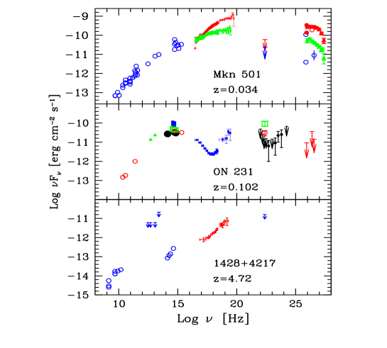
Figure 1: Examples of SED of blazars for which BeppoSAX observations were crucial. Adapted from Pian et. al. (1998), Tagliaferri et al. 2001 and Fabian et al. (2001)

2 The $\gamma$–ray zone

Observations of blazars at high energies showed a strong and (almost always) correlated variability of fluxes at the peaks of the SED. The first consequence of these results was to abandon the idea of a smooth inhomogeneous jet producing high frequencies at its base and lower frequencies in its outer part: most of the radiation we see should instead be produced in a single zone of the jet . In the following subsection I review the basic arguments leading to pinpoint the dimensions and the distance from the black hole of this “$\gamma$–ray zone”.

2.1 Low entropy inner jets

The very fact that blazars are strong $\gamma$–ray emitters implies that the produced $\gamma$–rays are not absorbed, and this in turn implies that:

1. the emitting source cannot be too compact, to avoid absorption of $\gamma$–rays through photon–photon collisions within the source;

2. the $\gamma$–ray emitting source cannot be too close to important sources of X–ray photons, such as a hot accretion disk corona, to avoid absorption of $\gamma$–rays with photons produced externally to the emitting region.

Point 1) leads to the requirement of bulk relativistic motion, since the observed compactnesses are large (i.e. huge luminosities and small dimensions as indicated by the short variability timescales, see e.g. Dondi & Ghisellini 1995). Point 2) leads to the requirement that the $\gamma$–rays we see are produced beyond a critical distance from the black hole and the accretion disk, which is likely to produce X–rays through its hot corona (Ghisellini & Madau 1996). Blandford (1993) and Blandford & Levinson (1995) introduced the concept of “$\gamma$–ray photosphere”, proposing a jet which dissipates energy also very close to the accretion disk. In this model the $\gamma$–rays produced within the $\gamma$–ray photosphere are absorbed and create pairs, loading the jet.

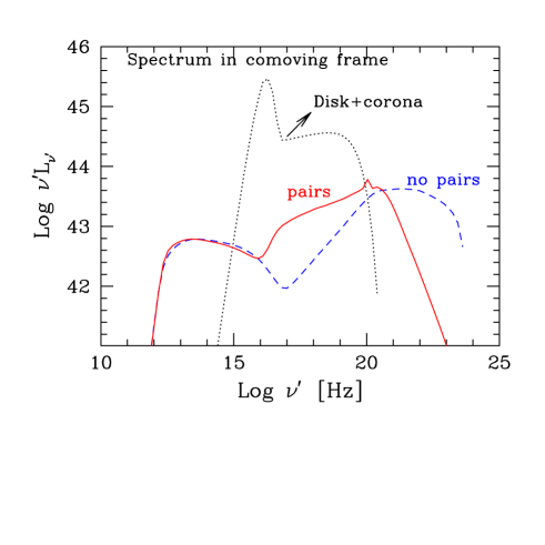
Figure 2: Synchrotron and Inverse Compton spectrum as observed in the frame comoving with the emitting blob, of radius $R=10^{15}$ cm moving with $\Gamma=15$. The blob is $10^{16}$ cm away from an accretion disk assumed to emit $\sim 10^{46}$ erg s^-1. Note how the pair cascade process significantly softens the spectrum, especially at X–ray frequencies.

In this case the jet is dissipative from its start. Ghisellini & Madau (1996) instead argued that the accretion disk, besides providing X–rays which interact with the $\gamma$–rays produced within the $\gamma$–ray photosphere, is producing UV radiation, which cools the just born relativistic pairs through the Inverse Compton process. In this case the pairs emit almost all their energy in (beamed) X–ray radiation, with a luminosity comparable to the observed $\gamma$–ray power. Since this is not observed, this process cannot occur: the jet therefore cannot dissipate much of its kinetic energy at small distances from the accretion disk. Fig. 2 illustrates this point. For simplicity, the optical-UV emission produced by the accretion disk is approximated with a blackbody, while the X–ray flux produced by the corona is assumed to be a power law (of energy index $\alpha_{x}=0.9$) ending with an exponential cut (dotted line in Fig. 2: the power is assumed to be calculated by an observer comoving with a blob moving with $\Gamma=15$). The blob is assumed to be spherical, with a size $R=10^{15}$ cm at a distance of $z=10^{16}$ cm from the accretion disk (whose relevant size is assumed to be $R_{\rm disk}\sim 3\times 10^{15}$ cm). The particle distribution responsible for the emission is calculated through the continuity equation, assuming continuous injection of elecrons distributed as a power law in energy between $\gamma_{1}=100$ and $\gamma_{2}=5\times 10^{3}$. We can see the effects of neglecting (dashed line) or including (solid line) pair production and pair reprocessing. All the energy absorbed in the $\gamma$–ray band is re–emitted, especially at X–ray energies. Observations show instead that in powerful blazars the flux in the X–ray range [2–10 keV] is particularly hard in shape and much much fainter than the $\gamma$–ray flux. We therefore conclude that in the presence of an accretion disk (producing cooling UV radiation) and its corona (producing X–ray photons, which are targets for the $\gamma$–$\gamma\to e^{\pm}$ process), the jet must transport its energy to a few hundreds of Schwarzchild radii before radiating.

On the other hand, the short variability timescales we observe, especially in the X–ray and $\gamma$–ray bands, constrain the size of the emitting region to be of the order of $\sim$1 light–day $\times\delta\sim 10^{16}$ cm or less, where $\delta$ is the Doppler factor. In a conical jet with aperture angle $\sim 0.1$, this dimension corresponds to a distance $z\sim 10^{17}$ cm from the black hole. We therefore conclude that there is a preferred distance where most of the dissipation is taking place.

2.2 No electron–positron pair cascades

The argument about the required absence of pair creation and pair reprocessing is more general than discussed above. In fact, also those models which invoke the existence of ultra–high energy protons, making pairs through interactions with optical–UV photons, face the problem of how to avoid pair cascades with the production of too many X–rays (see also Sikora & Madejski 2001). As an example, Fig. 3 shows the effects of neglecting/including the effects of pairs. For this model, I have assumed two different electron injection functions, one at low energies, responsible for the first peak of the SED through the synchrotron process, and another population of electrons at much higher energies, responsible for the second peak of the SED through, again, the synchrotron process. This second electron population should correspond to those leptons created through the proton–photon interactions, as envisaged in the “proton blazar” model by Mannehim (1993).

For illustration, the resulting spectra are compared to the SED of 0836+710, one of the most distant blazars detected by EGRET, with $z=2.17$. This source has a steep $\gamma$–ray spectrum, which cannot be the result of $\gamma$–absorption, since otherwise the created pairs would overproduce the X–ray flux even if any external radiation is absent and even if the dominant radiation mechanism is synchrotron, i.e. for magnetically dominated jets.

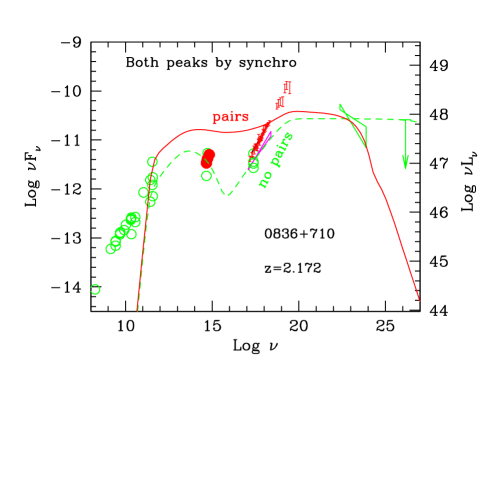
Figure 3: Pair cascades and the associated pair reprocessing can greatly affect the SED of a blazars. The reprocessing tends to fill in the “valley” between the two peaks of the SED. In this example, the spectrum is due to two different electron populations, with different high energy cut–offs and both peaks are due to synchrotron. The magnetic field is required to be large to avoid too much IC radiation (in this example $B=50$ G). If the high energy electrons were created through a pair–cascade of ultra–high energy photons, then too many X–rays would be produced.

3 The blazar sequence extended to low power BL Lacs

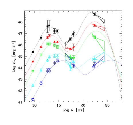
Figure 4: The blazar sequence. From Fossati et al. (1998) as modified by Donato et al. (2001).

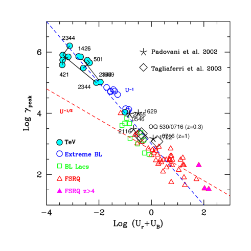
Figure 5: The random Lorentz factor of the electrons emitting at the peaks of the SED, $\gamma_{\rm peak}$, as a function of the comoving energy density (radiative plus magnetic). The dashed lines correspond to $\gamma_{\rm peak}\propto U^{-1/2}$ and $\propto U^{-1}$ (they are not best fits). From Ghisellini et al. (2002), updated with the data fom Padovani et al. (2002) and Tagliaferri et al. (2003).

Fossati et al. (1998), collecting data from three complete sample of blazars, demonstrated that the SED is controlled by the bolometric observed luminosity, with both peaks shifting at smaller frequences when increasing the luminosity (see Fig. 4). Furthermore, the dominance of the high energy peak increases when increasing the bolometric luminosity. This latter inference, however, was based on those few low power BL Lacs detected by EGRET. The new data coming from Cherenkov telescopes suggest instead that, in some cases, also in low power BL Lacs the high energy peak dominates the bolometric output, especially considering that the TeV emission could be severely absorbed by the diffuse IR background through the $\gamma$–$\gamma$ process (see e.g. Stecker & De Jager, 1997; for recent results on TeV sources see Aharonian et al. 2002, Costamante et al. 2003). This “blazar sequence” can be explained by a different degree of radiative cooling: in powerful blazars electrons cool faster, producing a break in the electron distribution functions at smaller and smaller energies when increasing the total (radiation plus magnetic) energy density in the comoving frame.

We (Ghisellini et al. 2002) extended the blazar sequence to include “extreme” BL Lacs, namely those low power BL Lacs which are the best candidate to be TeV emitters. Fig. 5 shows the random Lorentz factor emitting at the peaks of the SED as a function of the energy density as seen in the comoving frame. There are two branches: for “extreme” BL Lacs we have $\gamma_{\rm peak}\propto U^{-1}$, while for the other blazars $\gamma_{\rm peak}\propto U^{-1/2}$. Note that these behaviors corresponds, respectively, to a constant cooling time at $\gamma_{\rm peak}$ [i.e. $t_{\rm cool}(\gamma_{\rm peak})\propto(\gamma_{\rm peak}U)^{-1}$=const], or at a constant cooling rate at $\gamma_{\rm peak}$ [i.e. $\dot{\gamma}(\gamma_{\rm peak})\propto\gamma_{\rm peak}^{2}U=$ const].

We have interpreted this behavior by assuming that in all blazars the acceleration mechanism injects relativistic electrons between $\gamma_{1}$ and $\gamma_{2}$, but only for a finite time, which is of the order of the light crossing time of the source, $R/c$. In a powerful blazars all electrons cool in a timescale shorter than $R/c$, and the resulting particle distribution, after this time, has a break at $\gamma_{\rm peak}=\gamma_{1}$.

In low power BL Lacs, instead, only the very high energy particles can cool in $R/c$, and after this time the particle distribution will have a “cooling” break at some $\gamma_{\rm c}$ (with $\gamma_{\rm c}>\gamma_{1}$) which is the energy where the cooling time is equal to $R/c$, yielding $\gamma_{\rm peak}=\gamma_{\rm c}\propto U^{-1}$.

3.1 Variability above and below the peaks

A “snapshot” taken at the end of the injection time would catch a flare at its maximum. The assumption that the injection of particles lasts only for the finite time $R/c$ implies that the source would always vary on the timescale $\sim R/c$ (shortened by relativist effects) above the “cooling frequencies” $\nu_{\rm c}$ (namely the synchrotron and the inverse Compton frequencies produced by electrons with $\gamma>\gamma_{\rm c}$), while the flux below $\nu_{\rm c}$ should vary with the cooling timescale (i.e. with the characteristic $t_{\rm cool}\propto\nu^{-1/2}$ behavior).

This translates in a simple prediction: in low power BL Lacs, in which the peaks correspond to $\nu_{\rm c}$, we should see a characteristic variability behavior: at frequencies above the peaks of the SED the flux should vary with the same timescale, indicative of the size of the emission region, while at frequencies below the peaks the flux should vary with a timescale given by $ct_{\rm var}\delta\sim(R/c)(\nu_{\rm peak}/\nu)^{1/2}$, where $\delta$ is the Doppler factor.

In powerful blazars, instead, the peaks are determined by the injection energy $\gamma_{1}$, and not by $\gamma_{\rm c}$. This means that at frequencies both above and below the peak the flux should vary on the same timescale given by $ct_{\rm var}\delta\sim R/c$ .

4 Jet power

We believe that powerful blazars are associated with FR II galaxies, with prominent radio lobes. We can use equipartition arguments to find a minimum energy content in these structures, and by dividing it by the source lifetime we have an average power that the lobes require to exist. This is then a lower limit to the power of jets (Rawlings & Sanders 1991). This power is greater than the power radiated by the jet along its way, implying a small (i.e. 10 per cent) efficiency in converting bulk kinetic energy (or Poynting flux) into radiation. The jet energy carriers could be electrons and protons, electron–positrons pairs, or Poynting flux. Recently, the circular polarization discovered in the jet of 3C 279 by Wardle et al. (1998) led these authors to suggest that pairs are dominant, but later work (Ruszkowski & Begelman 2002) demonstrated that this is not necessarily the case. Another uncertainty is if the power of jets changes along the way, which is unlikely in powerful blazars and FR II, but perhaps possible in low power BL Lacs and FR I. It is therefore interesting to measure the power of jets at different scales. Up to now there are three jet scales where an estimate of the jet power is possible:

Figure 6: Distribution of jet powers for the blazars considered in Celotti & Ghisellini (2003). $L_{\rm p}$ is the power carried by protons assuming one proton per emitting electron; $L_{\rm e}$ is the power carried by the emitting electrons; $L_{\rm B}$ is the Poynting flux; $L^{\prime}_{\rm r}\Gamma^{2}$ is the power radiated by the jet and $L_{\rm e,cold}$ is the power carried in the form of electron rest mass (without including the relativistic random energy of the particles).

1. the $\gamma$–ray zone ($\sim$0.1 pc): this is the most dissipative zone, and we can measure the number of particles, the magnetic field, the size and the bulk Lorentz factor through the modeling of the SED (Ghisellini 2001; Ghisellini & Celotti 2002; Maraschi & Tavecchio 2003; Celotti & Ghisellini 2003);

2. the VLBI scale ($\sim$1–10 pc), where we can measure directly the apparent speed and the size (Celotti & Fabian 1993; Celotti et al. 1997);

3. the large scale jet ($\sim 10^{5}$ pc) as recently observed by Chandra in X–rays (Celotti et al. 2001, Tavecchio et al. 2000, Ghisellini & Celotti 2001a).

Fig. 6 shows the results obtained for the $\gamma$–ray zone by Celotti & Ghisellini (2003), considering all blazars with sufficient data to constrain the adopted model, which is a single zone synchrotron inverse Compton model with finite injection time. Due to the limited sensitivity of EGRET and Cherenkov telescopes, this implies that the SEDs we have modeled correspond to a flare state of the sources. Therefore the powers calculated in this way are probably upper values: to estimate the average powers one should know the duty cycle (i.e. the fraction of the time spent during flares). This will be possible with GLAST. From Fig. 6 we note:

• The estimated jet powers are large, and often exceed the power radiated by accretion (which can be estimated, in this beamed sources, through the luminosity of the emission lines).

• For powerful blazars (i.e. FSRQs sources) the power that the jet spends to produce radiation is in some case larger than the power carried in relativistic electrons responsible for the emission.

• Also the Poynting flux is often less then the radiated power. This is to be expected, since sources with a Compton flux dominating over the synchrotron flux cannot have large magnetic fields.

• If we assume that there is a proton for each electron, then the power carried by protons is a factor 10–30 larger than the radiated power, implying efficiencies of 3–10 per cent. In this case the remaining power can reach and energize the radio lobes.

• For low power BL Lacs, instead, there is not much difference between the power in electrons and in protons, since in these sources the average random Lorentz factors of the electrons is $\sim 1000$.

We then conclude that, at least in powerful blazars, the proton component of the jet must be energetically dominant (only 2 or 3 pairs per proton are allowed), unless the magnetic field present in the emitting region is only a fraction of what the jet transports.

5 Chandra jets

Chandra detected X–ray emission from knots in jets at distances of tens to hundreds kpc from the nucleus, both in powerful flat spectrum radio sources whose jet is probably aligned with the line of sight and in radio galaxies whose jets are instead observed at large viewing angles (see Tavecchio et al. 2003 and references therein).

For aligned jets the most popular interpretation of the observed X–ray emission is inverse Compton off the cosmic microwave background (CMB). This interpretation has also the virtue to minimize the energy requirements (Celotti et al. 2001; Tavecchio et al. 2000; Ghisellini & Celotti 2001a). This however requires the jets to be highly relativistic even at the largest scales: in the case of PKS 0637–712 the bulk Lorentz factor $\Gamma$ should still be 10–15, a few hundreds kpc away from the core. Bulk relativistic motion in fact implies that the CMB energy density is seen boosted by a factor $\sim\Gamma^{2}$ in the plasma comoving frame, and therefore can dominate over the local synchrotron and magnetic energy densities.

If this interpretation is correct, it also implies that the electrons producing the X–rays have random Lorentz factors of the order of one hundred with radiative cooling time much longer than the light crossing time. The optical and radio radiation, instead, is believed to be produced by synchrotron, by much more energetic electrons, with cooling times (for the optical) nicely coincident with the size of the knots, as measured by HST. Available observations then pose an interesting problem: outside the bright knots the X–ray flux is dimming as fast as the optical and radio fluxes, despite of the fact that it should be produced by low energy electrons, which do not cool radiatively. Do they cool by adiabatic losses? Is so, we then require several “doubling radii” to “switch off” the X–ray emission. The conclusion then is that the knot cannot be homogeneously filled with the emitting particles, but must be composed by smaller sub–units. In other words, the knot must be clumped: particles injected in each clump can then lose energy by adiabatic losses before reaching the borders of the knot, and produce a negligible amount of X–rays outside it (Tavecchio et al. 2003).

Note also that even if the electrons have lost their random energy once the reach the border of the knot, they still have bulk motion energy, and they continue to scatter CMB radiation. Such “large scale bulk Compton process” produces beamed radiation at frequencies $\nu\sim 3\times 10^{11}\Gamma^{2}$ Hz (the redshift dependence drops out), potentially detectable by ALMA. This could be a powerful test for the idea that these jets are relativistic up to large scales.

6 Internal shocks?

The result on the jet power and on the spectral modeling of blazars mentioned above can have a satisfactory explanation in the internal shock scenario, in which the central engine works intermittently producing blobs moving at slightly different velocities and therefore colliding at some distance from the black hole, transforming a few per cent of the bulk kinetic energy in radiation (see e.g. Ghisellini 1999; Spada et al., 2001). In fact this scenario easily explains:

• The fact that most of the dissipation occurs at $\sim$hundreds of Schwarzchild radii, which is the distance of the first collisions between consecutive shells;

• The observed variability, which is a built–in feature (but requires that the central engine works intermittently);

• The fact that we need particle acceleration lasting for a finite time, to explain the $\gamma_{\rm peak}-U$ correlation, since we have acceleration of particles for about one shell light crossing time;

• The fact that the jet produces radiation all along the way, but with a reduced efficiency. In fact, at large distances from the jet apex, shells that have already collided are moving with Lorentz factors which are intermediate of the original ones. These shell will collide further, but with a reduced contrast between their Lorentz factors, and therefore with a reduced efficiency.

• The blazar sequence, since the first energetic shell–shell collisions occur within the broad line region in powerful blazars, and outside the BLR in BL Lacs (if we assume that the BLR is located at a distance which correlates with the accretion disk luminosity, see e.g. Kaspi et al. 2000). In weak BL Lacs shell–shell collisions occur outside the BLR, in a much less dense external photon environment, implying less severe cooling (i.e. large $\gamma_{\rm peak}$) and a relatively more important SSC emission. Intermediate cases should exist, where the first collisions occurs sometimes within and sometimes outside the BLR. These sources should be characterized by a dramatic variability at high energies, such as observed in BL Lac itself (Bloom et al. 1997; Ravasio et al. 2002).

It is also a relatively simple scenario, allowing quantitative analysis (see Tanihata et al. 2002 for an application to Mkn 421). Besides all that, part of the appeal of this scenario lies on the possibility that $all$ relativistic jets work the same way, therefore including gamma ray bursts and galactic superluminal sources.

On the other hand, Blandford (2003) and Lyutikov & Blandford (2003) have proposed a purely electromagnetic jet, magnetically dominated. This contrasts with our distribution of Poynting fluxes for blazars, shown in Fig. 6, but this could be the results of having localized (clumped) emission regions where the magnetic field is less than the average (because of reconnection?). We need thus a way to distinguish between the two scenarios, bearing in mind that also in the internal shock scenario an acceleration mechanism is required, which might use magnetic forces. However, the matter has to achieve its final bulk Lorentz factor quite rapidly, before the $\gamma$–ray dissipation zone. One possibility to test the presence of a matter dominated jet might be to find a feature in the X–ray spectrum resulting from bulk Comptonization occurring at the base of the jet, as discussed by Sikora et al. (1997) and Sikora & Madejski (2003). In this case some excess emission is expected, at a frequency $\nu_{\rm disk}\Gamma^{2}\sim$1 keV, where $\nu_{\rm disk}$ is the peak frequency of the disk radiation.

7 Parent populations

It is commonly believed that BL Lac objects are aligned FR I sources, while the more powerful FSRQs are aligned FR II sources. This idea, originally put forward by Blandford & Rees (1978), has been tested by Urry and Padovani (see Urry & Padovani 1995 and references therein). Note that there can be “classical” BL Lacs (for instance: PKS 0537–441) which have line equivalenth widths less than the canonical 5 Å  value, but which have very luminous lines nevertheless: these could well be FSRQs with a particularly enhanced non–thermal continuum, and then belonging to the FR II class.

The recent possibility to determine the mass of the black hole through observations of the host galaxy made possible to investigate the black hole masses of both FR I and FR II, to see if they are different. We (Ghisellini & Celotti 2001b) considered the “Ledlow & Owen” (1996) plot, in which the two types of radio galaxies are neatly divided by a line in plane of radio luminosity vs optical luminosity of the host galaxy. In fact the optical luminosity of the host allows to estimate the black hole mass, while the radio luminosity correlates with the accretion disk luminosity. Fig. 7 shows the result: the dividing line between FR I and FR II is indistinguishable from the line corresponding to an accretion luminosity at the 0.6 per cent of the Eddington one. This bears the intriguing possibility that the diversity of jets is due to a property of the very nucleus of the AGN, and not to the different ambient into which the jet propagates. Namely, it is the accretion mode that could be different, since for ratios $L/L_{\rm Edd}<10^{-2}$ one expects that advection dominated accretion becomes important.

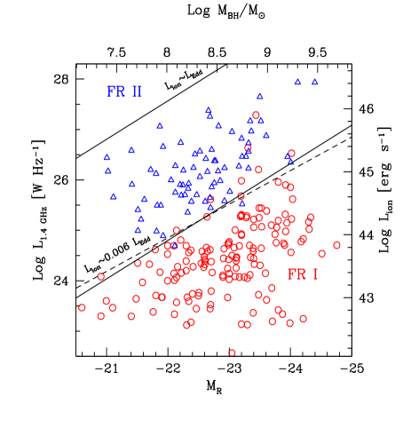
Figure 7: The radio jet power – host optical magnitude plane with the line sharply dividing FR I from FR II (dashed line, from Ledlow & Owen 1996). According to reasonably well established correlations this plane is equivalent to an accretion power vs black hole mass plane (right and upper axis). The central diagonal line represents $L_{\rm ion}\sim 6\times 10^{-3}L_{\rm Edd}$. From Ghisellini & Celotti (2002).

8 Conclusions

Extragalactic jets can have powers of the order of, but even greater then, what radiated by accretion. This is most clear in BL Lac objects, which lack any sign of the accretion activity, but can become dramatically evident if we consider gamma ray bursts (GRB) as jetted sources.

We are starting to understand the phenomenology of extragalactic jets, even if the issue of their formation, collimation and acceleration are still open. It is possible that blazar jets are similar to the jets of galactic superluminal sources and to the jets of GRBs. If true, it is very fruitful to study their similarities, differences, and the scaling laws. After all, the “internal shock” scenario was invented in the AGN field (Rees 1978), then it became the “standard” model to explain the prompt emission of GRBs, and it is again useful for blazars.

After the death of BeppoSAX and CGRO the observational prospects can become favorable again to blazar studies both by satellites (SWIFT, ASTRO–E2, and especially AGILE and GLAST) and by the new generation of ground based Cherenkov telescopes, (H.E.S.S., MAGIC, CANGAROO III and VERITAS), which should be a factor 10 more sensitive and have a smaller energy threshold, enabling them to detect distant (i.e $z>1$) sources. Blazars will be observed in all high energy bands almost without energy gaps, with very important consequences especially on cosmology, through the measurements they will allow on the IR through the UV cosmic backgrounds.

Acknwoledgments — It is a pleasure to thank Annalisa Celotti and Fabrizio Tavecchio for continuous interactions and collaborations.

References

- [1] Aharonian F. et al., 2002, A&A 403, 523
- [2] Blandford R.D. & Rees M.J., 1978, in “Pittsburgh Conference on BL Lac Objects”, (Pittsburgh Univ.) p. 328
- [3] Blandford R.D., 1993, AIP proc. 280, p. 533
- [4] Blandford R.D. & Levinson A., 1995, ApJ, 441, 79
- [5] Blandford R.D., 2003, in “The Physics of Relativistic Jets in the CHANDRA and XMM Era”, Bologna, in press.
- [6] Bloom S.D. et al., 1997, ApJ, 490, L145
- [7] Catanese M. & Weekes T.C., 1999, PASP, 111, 1193
- [8] Celotti, A. & Fabian, A.C. 1993, MNRAS, 264, 228
- [9] Celotti, A., Padovani, P. & Ghisellini, G., 1997, MNRAS, 286, 415
- [10] Celotti, A., Ghisellini, G. & Chiaberge, M. 2001, MNRAS, 321, L1
- [11] Celotti, A. & Ghisellini, 2003, in prep.
- [12] Costamante L. et al., 2003, in “TeV Astrophysics of extragalactic sources”, 2nd Veritas Symp, in press (astro–ph/0308025)
- [13] Donato D. et al. 2001, A&A, 375, 739
- [14] Dondi L. & Ghisellini G., 1995, MNRAS, 273, 583
- [15] Fabian A.C. et al., 2001 MNRAS, 324, 628
- [16] Ferrarese L. & Merrit D., 2000, ApJ, 539, L9
- [17] Fossati G. et al. 1998, MNRAS, 299, 433
- [18] Gebhardt K. et al., 2000, ApJ, 539, L13
- [19] Ghisellini G., 2001, ASP conf. eds. Giacconi R, Stella L. & S. Serio, 234, p. 425
- [20] Ghisellini G. & Madau P., 1996, MNRAS, 280, 67
- [21] Ghisellini G. et al., 1998, MNRAS, 301, 451
- [22] Ghisellini G., 1999, Astronomische Nachrichten, 320, p. 232
- [23] Ghisellini G., Celotti A. & Costamante L., 2002, A&A, 386, 833
- [24] Ghisellini G. & Celotti A., 2001a, MNRAS, 327, 739
- [25] Ghisellini G. & Celotti A., 2001b, A&A, 379, L1
- [26] Ghisellini G. & Celotti A., 2002, ASP Conf. Series, p. 273, (astro–ph/0108110)
- [27] Hartman, R.C. et al., 1999, ApJS, 123, 79
- [28] Kaspi S. et al., 2000, ApJ, 533, 631
- [29] Kormendy J. & Richstone D., 1995, ARAA, 33, 581
- [30] Ledlow M.J. & Owen F.N., 1996, AJ, 112, 9
- [31] Lyutikov M. & Blandford R.D., 2003, in “Beaming and Jets in Gamma Ray Bursts”, 2002, in press (astro–ph/0210671)
- [32] Magorrian J. et al., 1998, AJ, 115, 2285
- [33] Mannheim K., 1993, A&A, 269, 67
- [34] Maraschi L. & Tavecchio F., 2003, ApJ, 593, 667
- [35] Padovani P. et al., 2002, ApJ, 581, 895
- [36] Pian E., et al., 1998, ApJ, 491, L17
- [37] Rees M.J., 1978, MNRAS, 184, P61
- [38] Ravasio M. et al., 2002, A&A, 383, 763
- [39] Rawlings, S.G. & Saunders, R.D.E., 1991, Nature, 349, 138
- [40] Ruszkowski M. & Begelman M.C., 2002, ApJ, 573, 485
- [41] Sikora M. et al. 1997, ApJ, 484, 108
- [42] Sikora M. & Madejski G., 2001, in “High Energy Gamma–Ray Astronomy”, Eds. F. Aharonian and H. Voelk, AIP proc. 558, 275
- [43] Sikora M. & Madejski G., 2003, in “Active Galactic Nuclei: From Central Engine to Host Galaxy”, in press (astro–ph/0211587)
- [44] Spada M. et al., 2001, MNRAS, 325, 1559
- [45] Stecker F.W. & De Jager O.C., 1997, ApJ, 476, 712
- [46] Tagliaferri G. et al., 2001, A&A, 354, 431
- [47] Tagliaferri G. et al., 2003, A&A, 400, 477
- [48] Tanihata C. et al., 2003, ApJ, 584, 153
- [49] Tavecchio F., Ghisellini G. & Celotti A., 2003, A&A, 403, 83
- [50] Tavecchio F. et al., 2000, ApJ, 544, L23
- [51] Urry M.C. & Padovani P., 1995, PASP, 107, 803
- [52] Wardle J.F.C. et al., 1998, Nature, 395, 457