On Recovering the Nonlinear Bias Function from Counts in Cells Measurements

Abstract

We present a simple and accurate method to constrain galaxy bias based on the distribution of counts in cells. The most unique feature of our technique is that it is applicable to non-linear scales, where both dark matter statistics and the nature of galaxy bias are fairly complex. First, we estimate the underlying continuous distribution function from precise counts-in-cells measurements assuming local Poisson sampling. Then a robust, non-parametric inversion of the bias function is recovered from the comparison of the cumulative distributions in simulated dark matter and galaxy catalogs. Obtaining continuous statistics from the discrete counts is the most delicate novel part of our recipe. It corresponds to a deconvolution of a (Poisson) kernel. For this we present two alternatives: a model independent algorithm based on Richardson-Lucy iteration, and a solution using a parametric skewed lognormal model. We find that the latter is an excellent approximation for the dark matter distribution, but the model independent iterative procedure is more suitable for galaxies. Tests based on high resolution dark matter simulations and corresponding mock galaxy catalogs show that we can reconstruct the non-linear bias function down to highly non-linear scales with high precision in the range of $-1\leq\delta\leq 5$. As far as the stochasticity of the bias, we have found a remarkably simple and accurate formula based on Poisson noise, which provides an excellent approximation for the scatter around the mean non-linear bias function. In addition we have found that redshift distortions have a negligible effect on our bias reconstruction, therefore our recipe can be safely applied to redshift surveys.

1 Introduction

The principal aim of statistical analysis of galaxy catalogs is to extract information about the initial fluctuations in the early universe, their subsequent gravitational growth, and processes of galaxy formation. To decipher the available data, the distribution of the underlying dark matter have to be inferred from the distribution of galaxies. The two distributions in principle can be assumed to be quite different, i.e. galaxies are biased tracers of the underlying dark matter statistics (Kaiser, 1984; Bardeen et al., 1986; Lahav & Saslaw, 1992; Dekel & Lahav, 1999). In a class of phenomenological models, galaxy fluctuations $\delta_{g}$ are assumed to be a function of the matter fluctuation field, $f(\delta_{m})$, including the simplest case of linear bias $\delta_{g}=b\cdot\delta_{m}$ (Fry & Gaztañaga, 1993; Szapudi, 1995; Matsubara, 1995, 1999). Accurate knowledge of this function is needed to interpret galaxy statistics in light of theories of structure formation.

The bias function can be extracted from measurements of large scale structure statistics and Cosmic Microwave Background (CMB). One possibility is to use second order statistics from several sources, especially CMB maps together with galaxy catalogs to constrain bias (e.g. Efstathiou et al. 2002; Lahav et al. 2002; Verde et al. 2003). The underlying idea is that fluctuations in the CMB have a direct relationship with density fluctuations in the early universe. The comparison with present day galaxy statistics reveal information on both the gravitational amplification, and galaxy formation. The application of these methods is limited to fairly large scales, since non-linear growth and bias for galaxies, as well as secondary anisotropies for the CMB become more and more complex on smaller scales.

Another class of methods use higher order statistics (Fry & Gaztañaga, 1993; Gaztañaga & Frieman, 1994; Fry, 1994; Szapudi, 1998a; Feldman, Frieman, Fry, Scoccimarro, 2001; Verde et al., 2002) or velocity information (e.g. Branchini, Zehavi, Plionis & Dekel 2000; Zaroubi, Branchini, Hoffman & da Costa 2002) from galaxy catalogs to derive the bias function internally. These methods again are limited to linear to weakly non-linear scales, where both gravitational instability and bias theory is on a well understood. Since the most reliable large scale structure data are available on smaller scales, it is natural to seek methods for constraining bias, applicable on small, non-linear scales. The principal aim of this work is to introduce such technique based on a direct comparison of counts in cells in simulations and data.

We generalize a simple and elegant idea by Sigad, Branchini & Dekel (2000), based on the relation between the (continuous) cumulative probability distribution functions of the galaxy and matter density fluctuation fields, $C_{g}(\delta_{g})$ and $C_{m}(\delta_{m})$,

$$C_{m}(\delta_{m})=C_{g}(f(\delta_{m}))\ ,$$ (1)

where $C(\delta)\equiv\int_{-1}^{\delta}p(\delta^{\prime})d\delta^{\prime}$. The above relation allows in principle the recovery of the bias function, if both cumulative distributions are known:

$$\delta_{g}=f(\delta_{m})=C_{g}^{-1}\left[C_{m}(\delta_{m})\right]\ .$$ (2)

Sigad, Branchini & Dekel (2000) used an approximate form of this relation by simply replacing the cumulative probability distribution with the cumulative distribution of counts in cells $C_{N\leq N_{max}}=\sum_{N<N_{max}}P_{N}$, and postulating that the dark matter cumulative distribution is well described by a lognormal function. Both of these approximations render the original form of this method fairly approximate. Dark matter distribution does not exactly follow a lognormal distribution (as we show later), and discreteness effects (the difference between the continuous and discrete distribution) are important but for the densest galaxy catalogs. We improve the original idea on both counts: we measure the cumulative distribution for both galaxies, and for dark matter; the latter from simulations with the appropriate cosmology. In addition, we achieve accurate reconstruction of the continuous probability distribution function from the discrete counts in cells distribution. This eliminates most of the “stochastic” component of the bias arising from Poisson noise, and improves the accuracy of the reconstruction. Moreover, this means that we can penetrate smaller scales, where discreteness effects are important.

In what follows, we show that our method can recover the bias in a robust fashion with unprecedented precision, even in the non-linear regime. In the next section we present our method to estimate the continuous cumulative distribution function from discrete counts in cells measurements, and thus recover the bias function. In section three we test our technique in a suit of $N$-body simulations in both real and redshift spaces. The final section contains conclusions and discussions of our results.

2 Methods

The technical challenge of the idea outlined in the previous section consists of estimating the continuous probability distribution function from counts in cells measurements (CIC) in a robust way. Note that there are several proved and fast methods to estimate CIC distributions from galaxy catalogs or in simulations ( Szapudi 1998b; Szapudi, Quinn, Stadel & Lake 1999; Colombi & Szapudi 2003). In this work we are using the former method for all measurements.

The count probability distribution function (CPDF) $P_{N}$ is the probability that a certain cell has $N$ objects (galaxies). It is directly related to the continuous function under the locally Poissonian approximation

$$P_{N}=\int_{-1}^{+\infty}p(\delta)\frac{[\langle N\rangle(1+\delta)]^{N}e^{-\langle N\rangle(1+\delta)}}{N!}d\delta\ ,$$ (3)

where $\langle N\rangle$ is the mean CIC. Some models of galaxy formations predict sub-Poissonian scatter for very small halos (e.g. Somerville et al. 2001; Casas-Miranda et al. 2002; Berlind & Weinberg 2002). As long as a specific theoretical model, written in a convolution form similar to the above, is available, our technique can be easily adapted. For most scales, however, the local Poissonian assumption appears to be correct, and we assume it for the rest of this work.

As long as Eq (3) can be inverted, Eq (2) can be used to calculate the bias. The inversion, however, is a fairly delicate process. Most of the technical challenge of our aim was met by devising pair of new methods for deconvolving this somewhat unstable equation in a robust way.

2.1 Richardson-Lucy Deconvolution

To invert Eq (3) in a model independent way, we use the Richardson-Lucy (RL) method (see appendix C in Binney & Merrifield 1998 and reference there in). This iterative method is based on the Bayes theorem. The kernel in Eq.(3) is Poissonian

$$K(N,\delta)=\frac{[\langle N\rangle(1+\delta)]^{N}e^{-\langle N\rangle(1+\delta)}}{N!}\ .$$ (4)

Since $N$ is within $[0,N_{max}]$ in practice, the $K(N,\delta)$ has to be normalized to unity with respect to $N$. In the probabilistic spirit of this method, the functions need rescaling: $\hat{K}=K/\sum_{N}K$ and $\hat{p}=p\cdot\sum_{N}K$. Starting from an initial guess of $\hat{p}_{1}$, we can calculate $P_{N,1}$ via Eq.(3). From this, a better approximation of $\hat{p}$ is obtained,

$$\hat{p}_{2}=\hat{p}_{1}\sum_{N=0}^{N_{max}}\frac{P_{N}}{P_{N,1}}\hat{K}(N,\delta)\ .$$ (5)

This in turn is used as the input for the next iteration. The improvement of the fit $P_{N,i}$ after the $i^{th}$ iteration is quantified by the cost function $\chi^{2}=\sum_{N}(P_{N}/P_{N,i}-1)^{2}$, where $P_{N}$ is the measured CIC distribution. One caveat is the phenomenon of “over-learning”, when the recovered probability distribution starts to fit small fluctuations in the measured $P_{N}$. This can inject artificial features into the results after (too) many iterations. Numerical experiments indicate, that after about $10$ iteration the $\log\chi^{2}$ is becoming fairly small and changes little. The process is illustrated in Figure 1., where a lognormal model for the PDF was used to generate a CPDF curve with noise generated at $5\%$ level. The inverted PDF on the figure is fairly accurate after 12 iteration, while the results of 100 iterations clearly show the sign of over-learning. Figure 2. displays $\log\chi^{2}$ as a function of iteration: indeed, beyond 10-12 iteration it is hardly changing; this is the point of diminishing returns, after which over-learning kicks in. The displayed cost function is fairly typical, and we have found that an inspection of $\log\chi^{2}$ always allows a simple determination of a sensible stopping point. Because of the slow change in the cost function, the inversion is only logarithmically sensitive to finding the optimal number of iterations, therefore this prescription is fairly robust.

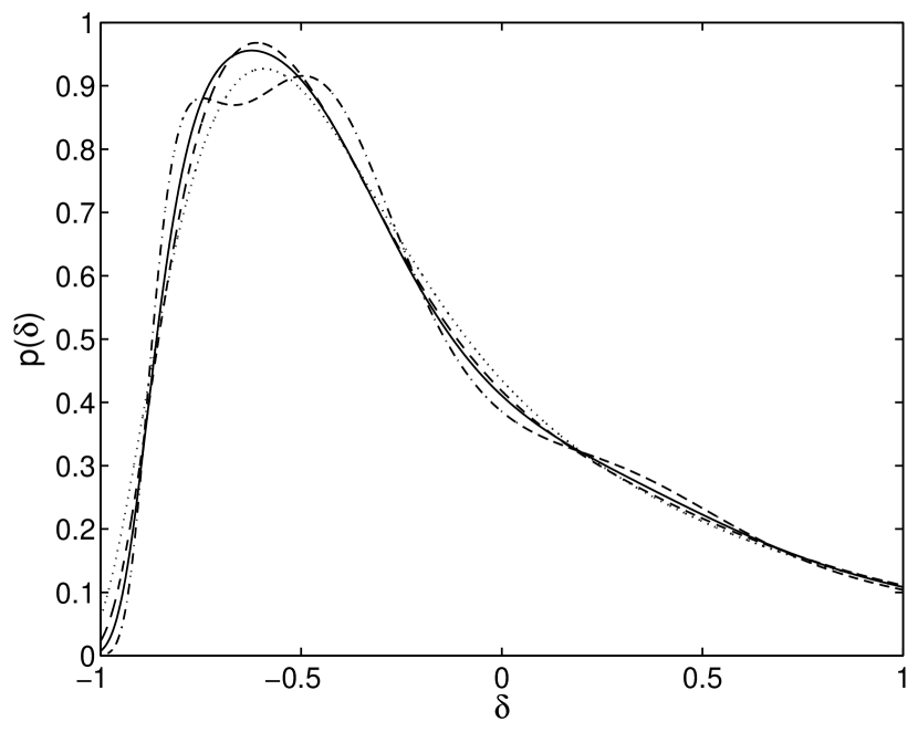
Figure 1: Richardson-Lucy inversion of an artificial PDf is plotted for a number of different iterations. The solid line corresponds lognormal input model from which the CPDF was generated according to Eq.(3). Noise was added to the CPDF at the $5\%$ level. The dotted line is the result after 5 iterations, the dash line corresponds to 12 iterations, while the dash-dots display 100 iterations. After 100 iterations over-learning problems appear (see Figure 2. as well)

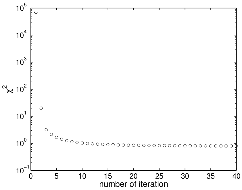
Figure 2: The cost function $\log\chi^{2}$ of the Richardson-Lucy method (see text) as a function of iterations for the example of Figure 1. Note that the change of the cost function becomes very slow after about 10-15 iterations, which would be a sensible stopping range for the iterations.

Numerical experiments show (see next section) that this method converges fairly fast and arrives at a robust result if $\langle N\rangle\lower 2.15277pt\hbox{$\;\buildrel>\over{\sim}\;$}0.1$. For smaller average counts convergence slows down such that a few 100 iterations are needed, as well as Poisson noise starts to dominate. We recommend that our method is used down to this value for robust results.

Another difficulty of the RL inversion is purely computational. Typically $N_{max}\sim 10^{4}$ for a CPDF of dark matter dataset from an N-body simulation, and the kernel is a broad function. For each pair of $N$ and $P_{N}$, we need to sample at least one point at the peak of the kernel $N/\langle N\rangle-1$, and a few hundred points on each side to keep the integration accurate. The last step thus costs about $10^{10}$ calculations of the kernel. Storing the kernel would require an array of floats of dimension $10^{4}\times 10^{6}$. This is unfeasible on a typical small workstation available to us. Similar computational problems arise with other direct inversion methods, such as singular value decomposition, etc. This motivates us to define an alternative, model-dependent method, which i) requires more modest computational resources, ii) it can extend toward even smaller scales, i.e. sparser sampling of the distribution.

2.2 Skewed Lognormal Model Fit

An alternative which naturally lends itself is to use physically motivated parametrized PDF models. This idea was explored by Kim & Strauss (1998),who adopted Gaussian Edgeworth expansions to the third order as model for $p(\delta)$ to deconvolve Eq.(3) and thereby fit for skewness and kurtosis. According to their investigations, such method is severely limited to the weakly non-linear regime, where the Gaussian Edgeworth expansion is good approximation. This is especially important in our application, where not only the first few moments are interesting, but the full behavior of the PDF containing information on very high order moments. Therefore we conclude that the Gaussian Edgeworth expansion is not a viable model for our purposes.

A more promising empirical model can be built based on the lognormal distribution (e.g. Coles & Jones 1991). This model is physically motivated, arising naturally from perturbation theory of the logarithm of the dark matter density field (Szapudi & Kaiser, 2003). Indeed, the skewed lognormal distribution (SLN3) appears to be an excellent approximation for the PDF of the dark matter field in a wide range of scales (Colombi, 1994; Ueda & Yokoyama, 1996). It is plausible then, that SLN3 might be a good approximation for galaxy distributions as well, as long as the bias is moderate; the tests of the next section indeed confirm this idea. Next we outline how one can proceed to invert Equation (3) under the assumption of SLN3.

With the notation $\rho=1+\delta$ (the density field), $\Phi=\log\rho-\langle\log\rho\rangle$ and $\sigma_{\Phi}=\langle\Phi^{2}\rangle$, the SLN3 model reads as

$$p_{3}(\delta)d\delta =\Big{[}1+\frac{1}{3!}T_{3}\sigma_{\Phi}H_{3}(\nu)+\frac{1}{4!}T_{4}\sigma_{\Phi}^{2}H_{4}(\nu)$$ (6)

$$+\frac{10}{6!}T_{3}^{2}\sigma_{\Phi}^{2}H_{6}(\nu)\Big{]}G(\nu)d\nu\ ,$$

where $\nu\equiv\Phi/\sigma_{\Phi}$, $H_{m}(x)$ is an Hermite polynomial of degree $m$, and $G(x)$ is a Gaussian with zero mean and variance of unity. The quantities $T_{3}$ and $T_{4}$ are the renormalized skewness and kurtosis of the field $\Phi$, respectively (Colombi, 1994):

$$T_{3}=\frac{\langle\Phi^{3}\rangle}{\sigma_{\Phi}^{4}}\ \ \ ,\ \ \ T_{4}=\frac{\langle\Phi^{4}\rangle-3\sigma_{\Phi}^{4}}{\sigma_{\Phi}^{6}}\ .$$ (7)

The convolution of $p_{3}(\delta)$ with the Poisson kernel, $\widetilde{P}_{N}$, corresponds to a model of observed $P_{N}$ depending on four parameters $\langle\log\rho\rangle$, $\sigma_{\Phi}$, $T_{3}$ and $T_{4}$. These parameters can be fitted to the observed distribution, which in turn yields the best approximation of the real PDF by $p_{3}(\delta)$. The following Poisson likelihood function was used to fit the parameters:

$${\mathcal{L}}=\prod_{N}\frac{(MP_{N})^{M\widetilde{P}_{N}}e^{-MP_{N}}}{(M\widetilde{P}_{N})!}\ ,$$ (8)

where $M$ be the total number of cells used for the CIC measurements. Minimization of $-\ln{\mathcal{L}}$ with respect to $\langle\log\rho\rangle$, $\sigma_{\Phi}$, $T_{3}$ and $T_{4}$ corresponds to a third order SLN fit, which is realized with the Powell’s method (Press et al., 1992).

Note that we have experimented with other cost functions for fitting the parameters, including the conventional minimal $\chi^{2}$ and a likelihood function of Kim & Strauss (1998), similar to the above, but $MP_{N}$ replaced with $M\widetilde{P}_{N}$. Numerical experience suggests that the above cost function, which is close to $\chi^{2}$ for large $MP(N)$, gives the best bias reconstruction among the variations tested.

3 Application to N-body Simulations

3.1 Simulations

The above described bias reconstruction method, including both inversion methods at its core, was extensively tested in a suit of the dark matter mock galaxy catalogs extracted from N-body simulations by the GIF project of the Virgo Consortium (Kauffman et al., 1999). We used the $z=0$ output for a LCDM universe with $\Omega_{m}=0.3$, $\Omega_{\Lambda}=0.7$, shape parameter, $\Gamma=0.21$, $\sigma_{8}=0.90$ and $h=0.7$, force soft length $20h^{-1}$kpc, the simulation box was of $L=141.3h^{-1}$Mpc. The simulations have $256^{3}$ particles of mass $1.4\times 10^{10}M_{\sun}h^{-1}$. We used two mock galaxy catalogs, the GIF galaxy catalog and the GIF galaxy catalog for SDSS. These artificial galaxy catalogs have been produced using semianalyical galaxy formation models (Kauffman et al., 1999; Somerville et al., 2000; Benson et al., 2000). They have been studied extensively to explore biasing as function of luminosity, scale and redshift by Somerville et al. (2001).

Because of the computational difficulty of the RL inversion for the large dark matter simulations, we used the SLN3 model fit exclusively for the inversion of the their PDFs. We found that above scales $2.21h^{-1}$Mpc SLN3 provides an excellent model for the dark matter distribution, while on smaller scales our model has more and more difficulty to fit the tail of the distribution (see Figure 3). On scales of 2.21 $h^{-1}$Mpc, the measured CPDF develops a very long tail even in log-space, which is not well fit by the polynomial correction of the SLN3 beyond $N>\sim 10^{3}$. However, since $\langle N\rangle=64$ and we aim to use our method up to $\delta<5$, we conclude that SLN3 will be a good approximation for our purposes.

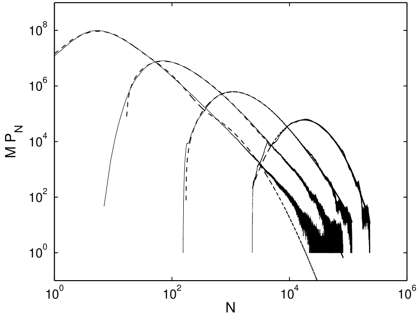
Figure 3: The CPDFs of the diluted dark matter sample on four different scales, from left to right, 2.21, 4.42, 8.83 and 17.66 $h^{-1}$Mpc. Solid lines show the measurements and dash lines represent our SLN3 model fits.

Table 1: parameters of SLN3 for the dark matter sample

Cell Size R ($h^{-1}$Mpc)	$\langle N\rangle$	$\langle\log\rho\rangle$	$\sigma_{\Phi}$	$T_{3}\sigma_{\Phi}$	$T_{4}\sigma_{\Phi}^{2}$
2.21	64	-1.157	1.185	1.110	1.289
4.42	512	-0.798	1.108	0.757	0.781
8.83	4096	-0.463	0.906	0.397	0.300
17.66	32768	-0.201	0.633	-0.008	-0.080

3.2 A null-test of bias reconstruction

In order to test the reliability of the bias extraction based on the SLN3 model fit, we selected several subsamples from the dark matter simulation by by randomly sampling them at 10%, 1% and 0.1%. The null-test consists of recovering $b=1$ from these catalogs; our method passed with flying colors.

As a typical example, fits to the measured CPDFs at 1% dilution level are presented on Figure 4. The fits are excellent approximation to the measurements. Then the recovered $C(\delta)$ is used to reconstruct the bias of our diluted subsamples with respect to the full sample. Except for $R=2.21h^{-1}$Mpc which has a $\sim 10\%$ peak difference, Figure 5. shows that the recovered bias is at most $\sim 5\%$ off from $b=1$ for $\delta<5$. We have performed the same study with several realizations, all giving similar results. The recovered bias at $R=2.21,4.42,8.83$ and $17.66h^{-1}$Mpc are $b=0.96\pm 0.12,1.02\pm 0.02,1.00\pm 0.03,$ and $1.01\pm 0.02$ respectively.

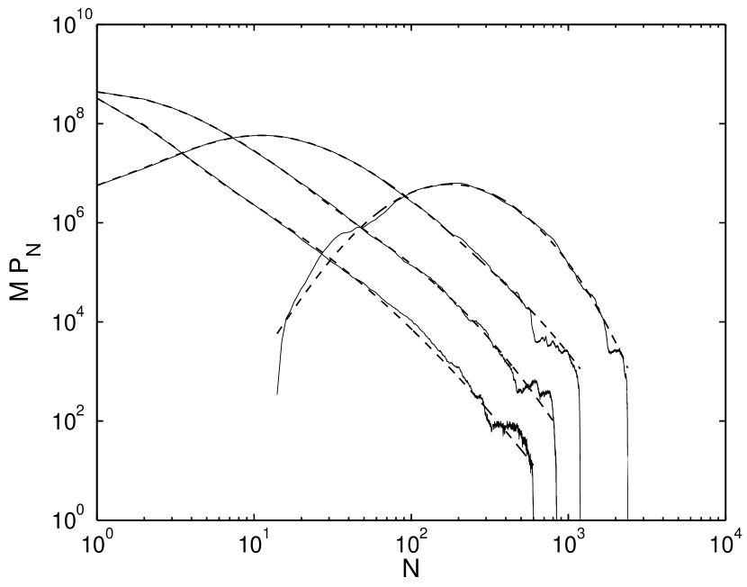
Figure 4: The CPDFs of the 1% diluted dark matter sample on four different scales of 2.21, 4.42, 8.83 and 17.66$h^{-1}$Mpc (from left to right). Solid lines correspond to our measurements, dash lines represent our model fits.

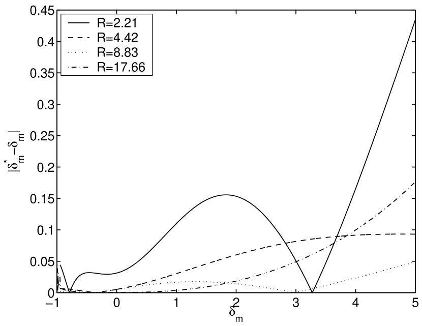
Figure 5: The deviation of the recovered bias function from $b=1$.$|\delta^{*}_{m}-\delta_{m}|=0$, where $\delta_{m}^{*}$ is the density fluctuation of the 1% diluted subsample, as a function of the density fluctuation $\delta_{m}$ of the full dark matter sample. Error-free reconstruction would yield 0. Both PDFs are generated by SLN3 model fits.

In addition, we have applied the Richardson-Lucy method to the 1% diluted subsamples. For $\delta<\sim 4$, the inverted PDFs are identical to the PDFs by SLN3 model fits except for the scale of $2.21h^{-1}$Mpc. Apparent differences occur at large $\delta$. When the SLN3 model PDF is used as a reference of the full dark matter sample, the bias parameter recovered by Richardson-Lucy inversion are 1.16, 1.04, 1.03, 0.94 on scales of $R=2.21,4.42,8.83,17.66h^{-1}$Mpc, respectively for $\delta<5$. From Figure 6. it is clear that on large scales both methods are in good agreement. On smaller scales the deviation is due to the domination of discreteness effects.

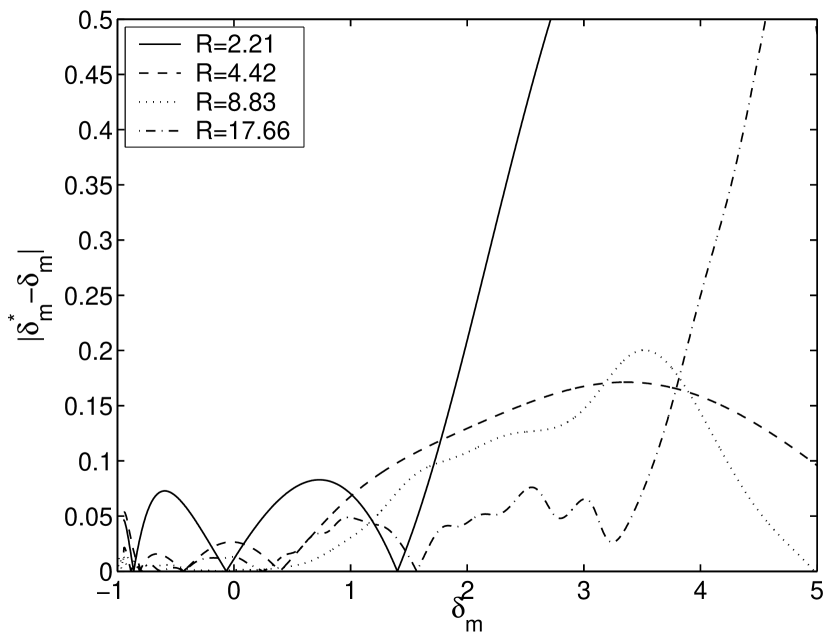
Figure 6: Same as Figure 5, except the PDFs of diluted subsample are inverted by Richardson-Lucy method, while the PDFs of the full dark matter simulation are still modeled by SLN3

3.3 Bias from the GIF Mock Galaxy Catalog

In this section we subject our method to extensive testing. We aim to recover the bias function between a GIF mock galaxy catalog and the underlying dark matter catalog. Since we have both catalogs (obviously not the case with real data), we can test our reconstruction against a density-density scatter plot based on a cell-by-cell comparison of the two catalogs. Note that such direct comparison contains significant Poisson scatter ( apparently the dominant contribution to stochastic bias). Our procedure recovers the main bias, since it is Poisson noise corrected.

Our SLN3 fits to CPDFs of the GIF galaxy catalog are shown in Fig.7. The corresponding cumulative PDFs of the galaxies and dark matter are displayed in Fig. 8. As we have seen in the previous section, SLN3 is a good approximation for the dark matter distribution. For the galaxy distribution, SLN3 fits the tail of the distribution less accurately, even on large scales. As long as the Poisson kernel is not too broad, we can still use the SLN3 fit as estimation of PDF for small $\delta$. We can estimate the limit of the applicability of the SLN3 estimation as $\delta_{max}\lower 2.15277pt\hbox{$\;\buildrel<\over{\sim}\;$}N_{max}/\langle N\rangle-1$, with $N_{max}$ being the $N$ where our fit breaks off from measured tail of the CPDF.

Cumulative PDFs based on the SLN3 model fit of the mock catalog and dark matter are shown in Fig.8. The bias function directly follows from Equation (1). We plot $\delta_{g}$ as function of $\delta_{m}$ in Fig.9. This is contrasted with the galaxy density-mass density scatter plot. Note that errorbars representing the scatter due to “stochastic bias”. The shaded area on the plot represents simple considerations for the stochasticity of the bias based on the assumption that all scatter is due to Poisson noise. It is an excellent approximation to the measured scatter (the errorbars), which appears to show that the scatter is indeed dominated by Poisson noise. We have checked that the measured errorbars are only weakly dependent on the bin width $\Delta\delta$, represented by horizontal errorbars: doubling it produced hardly noticeable effects. We have repeated the calculations using Richardson-Lucy method for the galaxies only, i.e. still SLN3 model for the dark matter. The bias function is displayed on Figure 9. with dash lines, except for the smallest scale, where $\langle N\rangle<0.1$ which we established as the limit of applicability of this method.

Table 2: parameters of SLN3 for the mock galaxy catalog

Cell Size R ($h^{-1}$Mpc)	$\langle N\rangle$	$\langle\log\rho\rangle$	$\sigma_{\Phi}$	$T_{3}\sigma_{\Phi}$	$T_{4}\sigma_{\Phi}^{2}$
2.21	0.059	-1.230	1.183	1.022	4.409
4.42	0.471	-1.318	1.591	0.752	-1.749
8.83	3.771	-0.769	1.389	-0.881	0.902
17.66	30.166	-0.250	0.798	-0.869	2.042

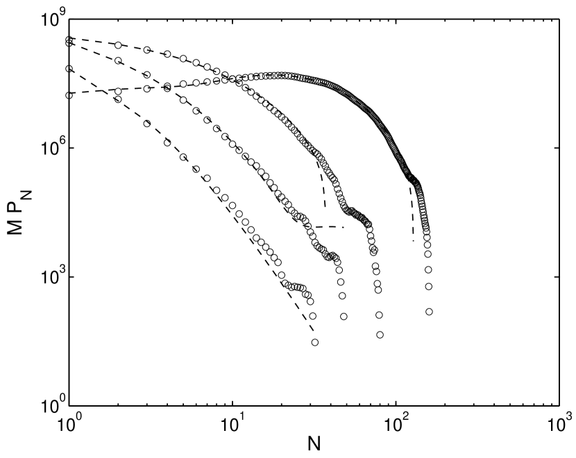
Figure 7: The CPDFs of the mock galaxy catalog on scales of 2.21, 4.42, 8.83 and 17.66$h^{-1}$Mpc (from left to right). Circles are measurements and dash lines are our SLN3 model fits.

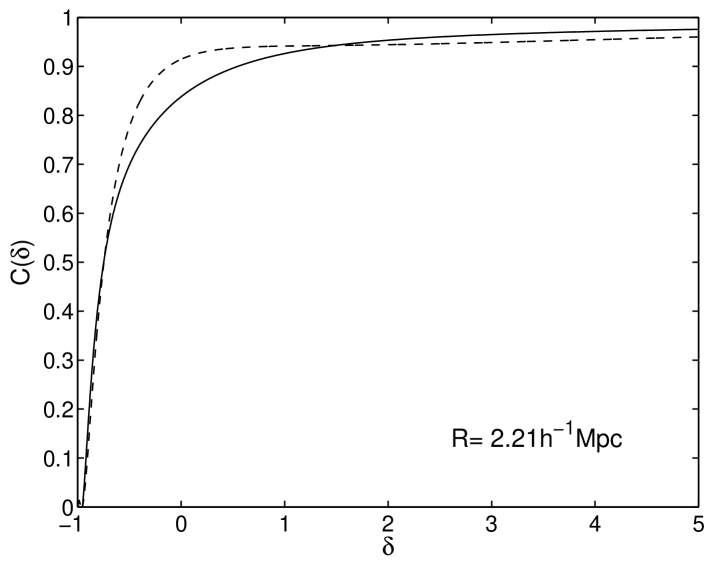
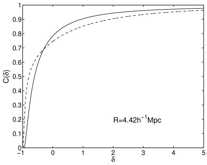
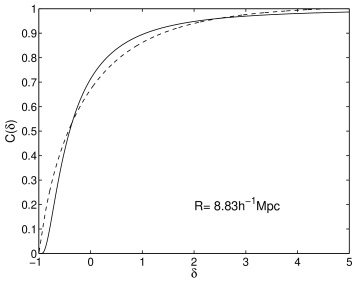
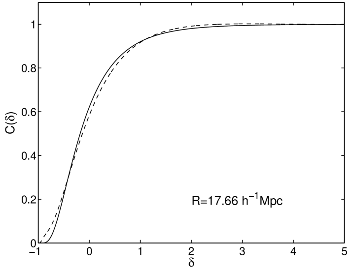
Figure 8: Cumulative PDFs fits based on SLN3 models of the mock galaxy catalog (dashed lines) and dark matter sample (solid lines).

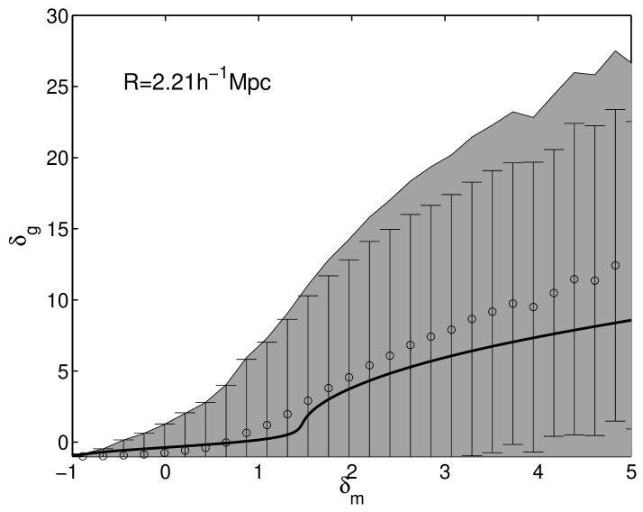
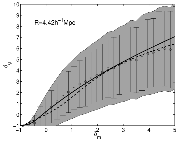
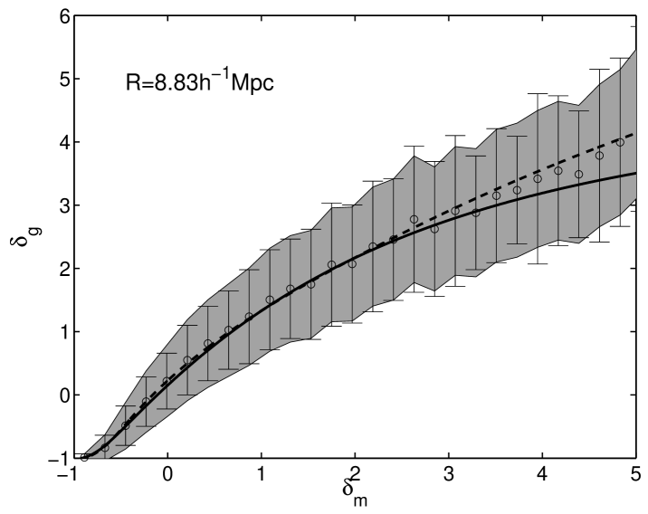
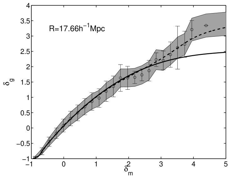
Figure 9: Bias function $\delta_{g}=f(\delta_{m})$ for the mock galaxy catalog. Solid lines are from the SLN3 model galaxy PDFs, dash lines are based on the Richardson-Lucy method. The reference mass PDFs were obtained from an SLN3 fit. Circles are the $\langle\delta_{g}|\delta_{m}\rangle$ measured directly from samples, errorbars show their $1\sigma$ scatter. The full width of $\delta_{m}$ bins of the scatter plot is $\Delta\delta_{m}=0.22$. The shaded area represents a simple Poisson scatter, which appears to be an excellent approximation to the stochasticity of the bias in these simulations.

3.4 Bias from the GIF Mock Galaxy Catalog for SDSS

This mock catalog contains more galaxies than the previous GIF mock galaxy catalog to match the density of the SDSS. The fits with SLN3 to its CPDFs are shown on Fig.10. Fitted parameters of the model are listed in Table 3. Bias functions are displayed in Fig.11.

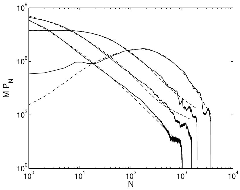
Figure 10: The CPDFs of the GIF mock galaxy catalog for SDSS on scales of 2.21, 4.42, 8.83 and 17.66$h^{-1}$Mpc (from left to right). Solid lines are from CIC measurements, dash lines are from SLN3 fit.

Table 3: parameters of SLN3 for the mock galaxy catalog for SDSS

Cell Size R ($h^{-1}$Mpc)	$\langle N\rangle$	$\langle\log\rho\rangle$	$\sigma_{\Phi}$	$T_{3}\sigma_{\Phi}$	$T_{4}\sigma_{\Phi}^{2}$
2.21	0.7198	-2.446	2.167	0.181	-0.300
4.42	5.758	-1.631	1.971	-0.387	0.557
8.83	46.064	-0.796	1.347	-0.338	0.968
17.66	368.514	-0.318	0.824	-0.231	0.280

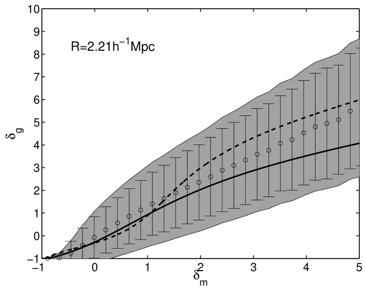
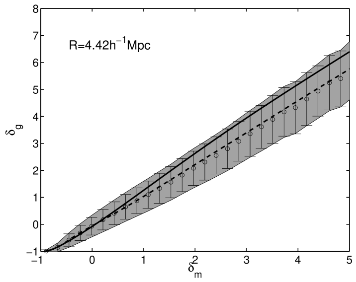
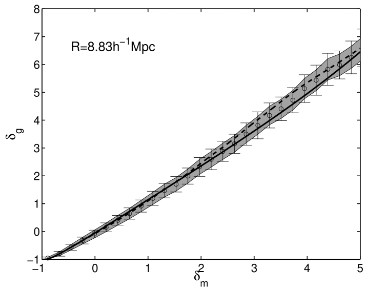
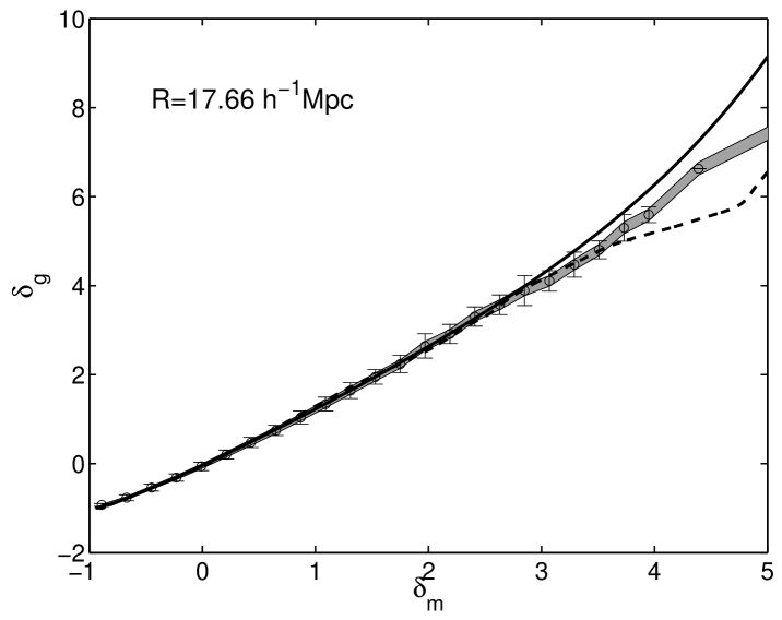
Figure 11: Same as Figure 9 but for the SDSS mock galaxy catalog.

3.5 Redshift space

All the tests we have done so far in real space have been repeated in redshift space. The plausible assumption about the application of our method in redshift space is that, in absence of significant velocity bias, the redshift space CPDFs will be modified similarly in the dark matter and galaxy catalogs. As long as this is correct, the bias function can be obtained by direct application of the method in redshift space. However, even if this assumption is only approximate, the dark matter distribution in redshift space is still recovered, which means that the effects of galaxy formation are decoupled from the evolution of dark matter; this is the principal goal of bias recovery. The tests in this section show that redshift distortions have a small effect on our procedure, thus our recipe can be safely applied to redshift surveys without significant corrections. It has to be born in mind though, that this statement is somewhat model dependent; we assume that the simulations and the semianalytic models used to create mock catalogs are close enough to reality that this statement will hold for real data.

The CPDFs and their SLN3 fits for the dark matter sample, the GIF mock galaxy catalog and the mock galaxy catalog for SDSS are shown in Fig.12, Fig.13 and Fig.14 respectively. The recovered bias functions of the GIF mocks galaxy are displayed in Fig.15, while for the SDSS mocks in Fig.16.

The recovery of bias in redshift space is just as successful as in real space. We have also compared the recovered red shift space bias function to that of the real space. Results based on RL inversion only are shown on Figure 17 (GIF galaxy mock catalog) and Figure 18 (mock galaxy catalog for SDSS). The difference between the two curves is generally small, in fact for $\delta_{m}\lower 2.15277pt\hbox{$\;\buildrel<\over{\sim}\;$}2$, the effect of redshift distortions on the bias function is negligible. The apparent difference between the GIF curves on scale of $4.42h^{-1}$Mpc is mostly due to the fact that the RL inversion is pushed to its limits at $\langle N\rangle=0.47$.

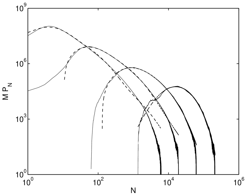
Figure 12: CPDFs and their SLN3 model fits for the dark matter in redshift space. Solid lines correspond to the measurements, while dash lines show SLN3 model fits. For these curves from left to right, cells size at which CPDFs are measured are $R=2.21,4.42,8.83,17.66h^{-1}$Mpc.

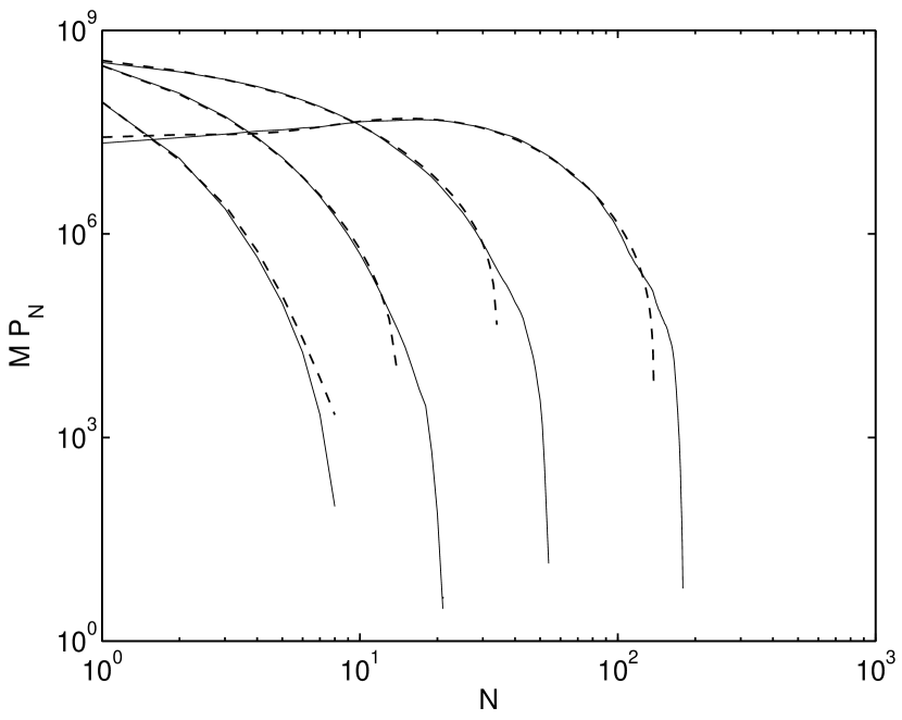
Figure 13: Same as Figure 12. but for the the GIF mock galaxy catalog in redshift space.

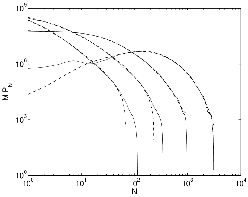
Figure 14: Same as Figure 12. but for the GIF mock galaxy catalog for the SDSS in redshift space

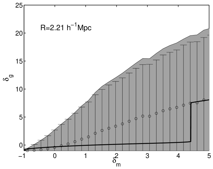
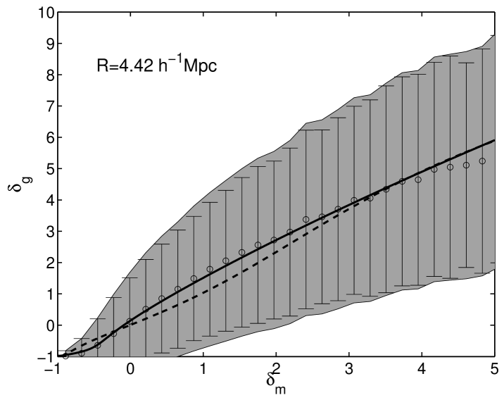
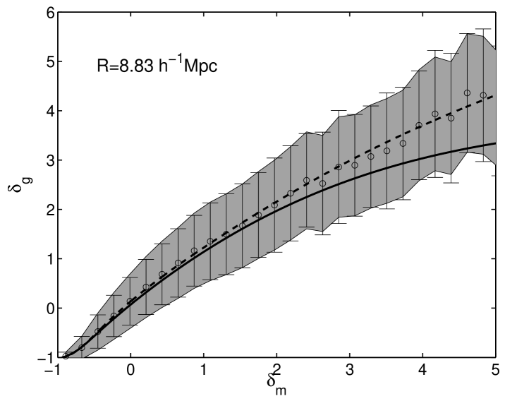
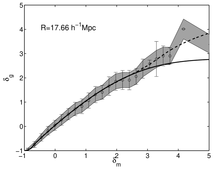
Figure 15: Same as Figure 9. but for the GIF galaxy catalog in redshift space.

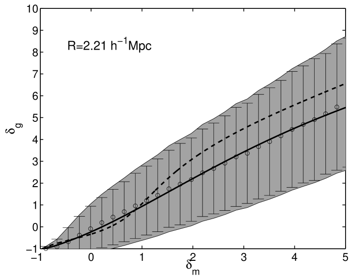
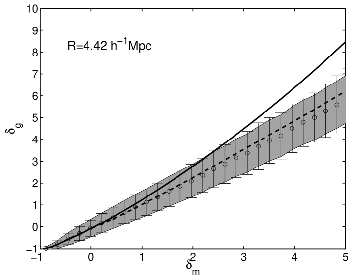
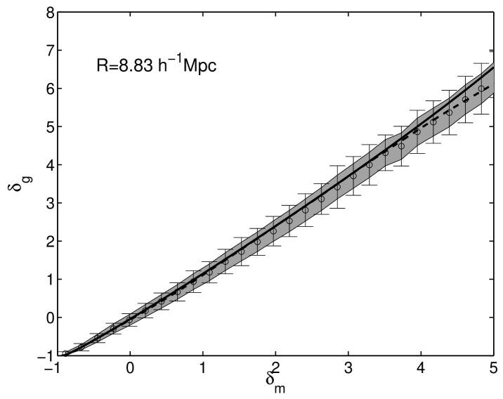
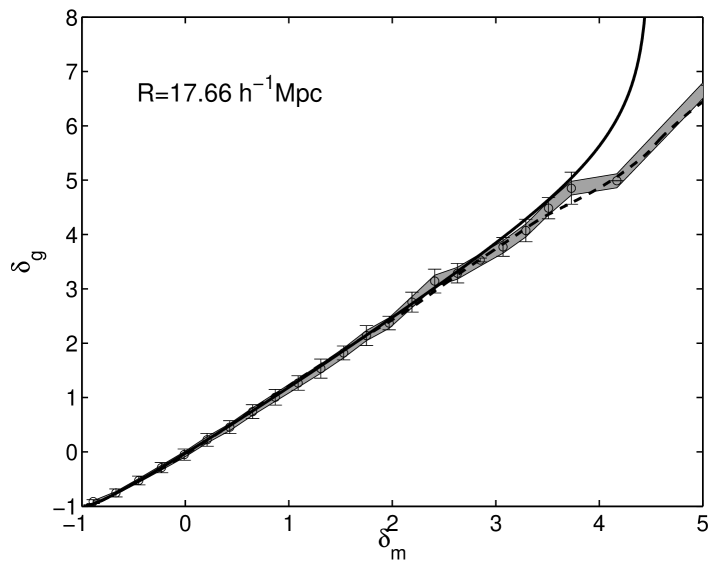
Figure 16: Same as Figure 9. but for the GIF mock galaxy catalog for the SDSS in redshift space

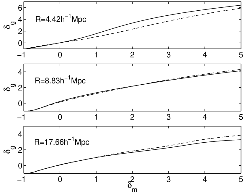
Figure 17: Comparison of recovered bias functions of the GIF galaxy catalog in real space (solid lines) and in redshift space (dashed lines).

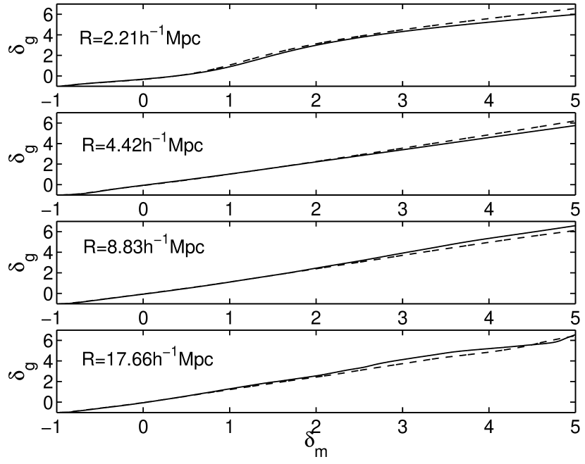
Figure 18: Same as Figure 17, but for the mock galaxy catalog for the SDSS.

4 Conclusion and Discussion

We have presented a new method to extract the bias function from galaxy catalogs. Since our method uses direct comparison statistics extracted from simulations and data, it is applicable to a large range of scales. In particular, its domain of validity includes the nonlinear regime, which has proved to be impenetrable to other previous methods. This is all the more important, since the most reliable data are still available on non-linear scales. In addition, most available data pushing to the largest scales have still significant non-linear “contamination”, to which our method is completely insensitive. In addition to expanding the range of applicability, our method has an accuracy which rivals all other methods. This is due to the fact, that it is using the full counts in cells distribution, which is sensitive to very high order statistics.

The new technique is based on comparing the cumulative probability distribution functions in simulations and data. To turn this idea into a robust and reliable method, a difficult technical challenge had to be met: the reconstruction of the continuous probability distribution of density fluctuations from counts in cells measurements. This is a delicate, and potentially unstable inversion, for which we have proposed two solutions. One is a model independent inversion using a Richardson-Lucy iteration, while the other is model dependent fit based on the skewed lognormal approximation (SLN3). The former method is useful down to scales where $\langle N\rangle\lower 2.15277pt\hbox{$\;\buildrel>\over{\sim}\;$}0.1$, and for relatively smaller number of particles due to computational constrains. The SLN3 fitting is useful possibly to even slightly smaller scales, and it is feasible for large simulations of arbitrarily high particle number. Therefore the former lends itself naturally for fitting the CPDF in galaxy catalogs, while the latter for large simulations. The range of reconstruction of the bias function is $-1\leq\delta\leq 5$, and typically we could recover the bias from fairly realistic simulations at the $5\%$ level. This suggests that our appication of our method to contemporary catalogs, such as the SDSS and 2dF, will constrain bias at an accuracy close to the absolute limit determined by systematic errors.

Most of our efforts have been centered on reconstructing the bias function itself represents the mean bias. We have found, however, that part of the scatter is at least, perhaps dominantly, due to Poisson scatter. Our reconstruction method corrects for this source of error to the fullest possible extent. In addition, we have found that a simple shot noise model gives excellent approximation to the stochastic component of the bias.

The expected number of galaxies in region with galaxy density fluctuation is $\delta_{g}$ is simply $N_{g}=\langle N_{g}\rangle(1+\delta_{g})$. If we assume a Poisson variance around this value (and neglect discreteness in the dark matter catalog which is a good approximation) we have

$$\frac{\Delta N_{g}}{N_{g}}=\frac{\Delta\delta_{g}}{1+\delta_{g}}=\frac{1}{\sqrt{\langle N_{g}\rangle(1+\delta_{g})}}\ .$$ (9)

It follows that $\Delta\delta_{g}=\sqrt{(1+\delta_{g})/\langle N_{g}\rangle}$. This simple formula is shown in Figure 9, 11, 15 and 16 as a shaded area and provides an approximation to the errorbars at typically at the 10% level, with the largest deviation being 50%, mainly at large $\delta$. It appears that Poisson scatter provides the dominant fraction of the stochasticity of the bias. Note that there are signs of sub-Poisson scatter in some of the Figures. The above is hardly more than a toy model, and its degree of success is remarkable.

A convenient parametrization of the (mean) bias function relies on a Taylor series expansion,

$$\delta_{g}=f(\delta_{m})=\sum_{k=0}^{\infty}\frac{b_{k}}{k!}\delta_{m}^{k}\ .$$ (10)

We adopted this form to fit our results empirically from the GIF and GIF-SDSS mock catalogs for $\delta_{m}\in[-1,5]$. We have found that an expansion up to $k=2$ is always sufficient. The results, based on RL inversion, are shown in Table 4 & 5. It also quantifies the difference between redshift and real space. For instance, $b=b_{1}$ is typically within a few percent for the two cases.

A subtlety with the above formula is worth emphasizing again: in this paper we have related the smoothed galaxy density field to the smoothed dark matter density field. Other methods might use “unsmoothed” field, which really means that smoothing is done on a much smaller scales than those scales considered in the measurement. The meaning of a truly unsmoothed galaxy density field, let alone its Taylor series expansion in terms of a truly unsmoothed dark matter density field is somewhat dubious. As well known, bias and smoothing does not commute, which means that our bias coefficients might have slightly different meaning than the quantities notated with the same letters in other works.

Table 4: Bias parameters for the GIF galaxy catalog

	In Real Space				In Redshift Space
R($h^{-1}$Mpc)	$b_{0}$	$b_{1}$	$b_{2}/2!$		$b_{0}$	$b_{1}$	$b_{2}/2!$
4.42	0.17	1.71	-0.085	$\cdots$	0.0029	1.15	0.016
8.83	0.16	1.18	-0.081	$\cdots$	0.10	1.17	-0.066
17.66	0.025	0.96	-0.062	$\cdots$	0.022	1.00	-0.047

Table 5: Bias parameters for the mock SDSS galaxy catalog

	In Real Space				In Redshift Space
R($h^{-1}$Mpc)	$b_{0}$	$b_{1}$	$b_{2}/2!$		$b_{0}$	$b_{1}$	$b_{2}/2!$
2.21	-0.14	1.55	-0.052	$\cdots$	-0.11	1.57	-0.037
4.42	-0.071	1.12	0.01	$\cdots$	-0.084	1.10	0.032
8.83	-0.062	1.20	0.032	$\cdots$	-0.038	1.19	0.013
17.66	-0.015	1.20	0.059	$\cdots$	0.005	1.19	0.014

No statistical method would be complete without a way of placing errorbars on the estimates derived from the method. Since our method is fully non-linear and it relies on direct comparison of galaxy catalogs with simulations, the only robust way of producing errorbars is a Monte Carlo estimate. The procedure is obvious: one has to repeat all the calculations using a suit of simulations representing the data. As matter of fact, we have demonstrated this in section 3.2, when we have measured bias in several realizations of the randomly diluted samples. If the dark matter simulation is large and dense enough, most of the variance will come from data. While for most of our present investigation only one realization was at our disposal, the CPU budget would allow the analysis of a large number of simulations. It took about one hour to measure CIC in dark matter and galaxy catalogs, about 30 minutes for one SLN3 fit, and up to a few hours for RL inversion (typical value in our calculation of the mock SDSS). We have used a 2.4GHz dual Xeon workstation with 2GBytes of memory.

In this work we exclusively used the Poisson model to relate the discrete galaxy distribution to the underlying continuous field. This approximation might break down, especially on very small scales, where halo models are known to predict sub-Poisson scatter (Casas-Miranda et al., 2002; Berlind & Weinberg, 2002). Such theories, once firmly established, can be naturally incorporated into our formalism via simply generalizing the kernel. Another application, where the kernel will need modification is recovery of the bias from two dimensional angular catalogs. In that case the corresponding kernel would depend on the selection function, but the core idea of the method would still work. These generalizations as well as applications to real data are in preparation.

References

- Bardeen et al. (1986) Bardeen, J., Bond, J. R., Kaiser, N., & Szalay, A. 1986, ApJ, 304, 15
- Benson et al. (2000) Benson, A. J., Cole, S., Frenk, C. S., Baugh, C. M. & Lacey, C. G., 2000, MNRAS, 311, 793
- Berlind & Weinberg (2002) Berlind, A. A. & Weinberg, D. H., 2002, ApJ, 575, 587
- Binney & Merrifield (1998) Binney, J. & Merrifield, M., 1998, Galactic Astronomy, Princeton University Press, Princeton
- Branchini, Zehavi, Plionis & Dekel (2000) Branchini, E.; Zehavi, I.; Plionis, M. & Dekel, A., 2000, MNRAS, 313, 491
- Casas-Miranda et al. (2002) Casas-Miranda, R., Mo, H. J., Sheth, Ravi K., & Boerner, G., 2002, MNRAS, 333, 730
- Coles & Jones (1991) Coles, P. & Jones, B., 1991, MNRAS, 248, 1
- Colombi (1994) Colombi, S., 1994, ApJ, 435, 536
- Colombi & Szapudi (2003) Colombi, S. & Szapudi, I., 2003, in preparation
- Dekel & Lahav (1999) Dekel, A. & Lahav, O., 1999, ApJ, 520, 24
- Efstathiou et al. (2002) Efstathiou, G., et al., 2002, MNRAS, 330, L29
- Feldman, Frieman, Fry, Scoccimarro (2001) Feldman, H. A., Frieman, J. A., Fry, J. N., Scoccimarro, R., 2001, PhRvL, 86, 1434
- Fry (1994) Fry, J.N., 1994, PhRvL., 73, 215
- Fry & Gaztañaga (1993) Fry, J.N. & Gaztañaga, E., 1993, ApJ, 413, 447
- Gaztañaga & Frieman (1994) Gaztañaga, E. & Frieman, J. A., 1994, ApJ, 437, 13
- Kaiser (1984) Kaiser, N. 1984, ApJ, 284, L9
- Kauffman et al. (1999) Kauffman, G., Colberg, J. M., Diaferio, A., & White, S. D. M., 1999, MNRAS, 303, 188
- Kim & Strauss (1998) Kim, R. S. J. & Strauss, M. A., 1998, ApJ, 493, 39
- Lahav & Saslaw (1992) Lahav, O., & Saslaw, W. 1992, ApJ, 396, 430
- Lahav et al. (2002) Lahav, O., et al., 2002, MNRAS, 333, 961
- Matsubara (1995) Matsubara, T., 1995, ApJS, 101, 1
- Matsubara (1999) Matsubara, T., 1999, MNRAS, 525, 543
- Press et al. (1992) Press, W. H., Flannery, B. P., Teukolsky, S. A., & Vetterling, W. H. 1992, Numerical Recipes, The Art of Scientific Computing (2nd ed.), Cambridge Univ. Press, Cambridge