A Spectroscopic Technique for Measuring Stellar Properties of Pre–Main Sequence Stars

Abstract

We describe a technique for deriving effective temperatures, surface gravities, rotation velocities, and radial velocities from high resolution near–IR spectra. The technique matches the observed near–IR spectra to spectra synthesized from model atmospheres. Our analysis is geared toward characterizing heavily reddened pre–main sequence stars but the technique also has potential applications in characterizing main sequence and post–main sequence stars when these lie behind thick clouds of interstellar dust. For the pre–main sequence stars, we use the same matching process to measure the amount of excess near–IR emission (which may arise in the protostellar disks) in addition to the other stellar parameters. The information derived from high resolution spectra comes from line shapes and the relative line strengths of closely spaced lines. The values for the stellar parameters we derive are therefore independent of those derived from low resolution spectroscopy and photometry. The new method offers the promise of improved accuracy in placing young stellar objects on evolutionary model tracks. Tests with an artificial noisy spectrum with typical stellar parameters, and signal–to–noise of 50 indicates a 1$\sigma$ error of 100 K in T_eff, 2 km s^-1 in $v\sin i$, and 0.13 in continuum veiling for an input veiling of 1. If the line flux ratio between the sum of the Na, Sc, and Si lines at 2.2 $\mu$m and the (2–0) ¹²CO bandhead at 2.3 $\mu$m is known to an accuracy of 10%, the errors in our best fit value for $\log g$ will be $\Delta\log g$ = 0.1–0.2. We discuss the possible systematic effects on our determination of the stellar parameters and evaluate the accuracy of the results derivable from high resolution spectra. In the context of this evaluation, we explore quantitatively the degeneracy between temperature and gravity that has bedeviled efforts to type young stellar objects using low resolution spectra. The analysis of high resolution near–IR spectra of MK standards shows that the technique gives very accurate values for the effective temperature. The biggest uncertainty in comparing our results with optical spectral typing of MK standards is in the spectral type to effective temperature conversion for the standards themselves. Even including this uncertainty, the 1$\sigma$ difference between the optical and IR temperatures for 3000–5800 K dwarfs is only 140 K. In a companion paper (Doppmann, Jaffe, & White, 2003), we present an analysis of heavily extincted young stellar objects in the $\rho$ Ophiuchi molecular cloud.

1 Introduction

Our understanding of main sequence and post main sequence stellar evolution is a triumph of collaboration between theorists building physical models and observers collecting precise observations. Over many decades, the two groups have compared their results on the common ground of the Hertzsprung–Russell (H–R) diagram. For young stellar objects (YSOs) however, the link between theory and observation is much more tenuous.

There is a well–developed empirical scheme that classifies YSOs by their broad–band spectral energy distributions (Lada, 1987). Class I sources have rising near– to mid–IR spectra. Class II sources have broad, largely flat infrared spectral energy distributions, and Class III sources have spectral energy distributions of hot reddened blackbodies. Since the emission that distinguishes Class I and II objects from Class III sources does not arise from the stellar photosphere, models of pre–main sequence (PMS) evolution are not strongly constrained by matching theoretical and observed spectral energy distributions. Comparison of model tracks with observational H–R diagrams has been possible for visible T Tauri (Class II) stars (TTSs) (e.g. Huang, 1961; Stahler, 1988; Hatmann et al., 1991; Kenyon & Hartmann, 1995; White et al., 1999; Webb et al., 1999; Simon et al., 2000; White & Ghez, 2001). Obscuration by dust makes it difficult to study Class I objects and to observe TTSs in the visible if these objects are in clusters or associations within molecular clouds. The resulting difficulties in comparing tracks with observations leave our understanding of the physics of YSOs on a much less solid footing than our understanding of more evolved objects.

In studying YSOs, our main goal is to understand the history of these objects from their formation to their arrival on the main sequence. We also wish to use the ensemble of such objects to characterize forming clusters and associations; their initial mass functions and star formation histories. To meet these goals, we need to determine parameters of the stars and relate them to other properties of protostellar disks and of the surrounding cloud. The most important stellar parameters to obtain are the effective temperature and the luminosity or surface gravity since this pair permits us to place the YSOs into a theoretical H–R diagram for comparison with theoretical PMS evolution models. (Note that luminosity and $\log g$ are not fully interchangeable since the relationship between these two quantities depends on the not yet well established mass–luminosity–radius relationship for YSOs.) Other useful parameters include the amount of reddening or extinction, the amount of non–photospheric emission as a function of wavelength, and the stellar rotation rate.

Observers have used many techniques to investigate the properties of stars in very young embedded clusters. In well–studied regions like the $\rho$ Ophiuchi cloud core, previous investigators have used photometric surveys in the near–IR (Wilking & Lada, 1983; Greene & Young, 1992; Barsony et al., 1997), in the mid–IR (Bontemps et al., 2001), and low–to–moderate resolution ($R\equiv\lambda/\Delta\lambda=$ 500–2000) near–IR spectroscopy (Casali & Matthews, 1992; Greene & Meyer, 1995; Greene & Lada, 1996; Kenyon et al., 1998; Luhman & Rieke, 1999), to estimate temperatures, luminosities, and the amount of excess (non–photospheric emission) in the infrared for the sources. In embedded clusters, however, even near–IR photometry and low resolution spectroscopy suffer under disadvantages not inflicted upon these techniques when applied to main sequence stars or to less heavily extincted young stars. Problems include extremely high extinction (e.g. the central part of the $\rho$ Ophiuchi molecular cloud where $A_{\rm v}=40\pm 10.9$ magnitudes, Luhman & Rieke, 1999), and excess emission in the near– and mid–IR (from warm dust in the circumstellar disks, Greene et al., 1994; Strom et al., 1995).

Observers recognized long ago that spectral classification in the near–IR was a potentially valuable tool for deriving the properties of obscured stars in the Galactic Plane and young stars obscured by their natal clouds (Merrill & Ridgway, 1979). Young stars are brighter in the infrared both because their photospheres tend to be cool and because it is easier for the stellar infrared emission to penetrate through the dust within the star forming cloud or along the line–of–sight. Also, in TTSs, the ratio of photospheric flux to the hot continuum that produces the excess emission frequently seen in the UV (presumably from accretion shocks, Gullbring et al., 2000) is higher in the infrared than at shorter wavelengths, permitting better detections of photospheric lines.

The near–IR spectra of late–type stars contain useful information about the luminosities of the targets. The strength of the CO overtone bands at 2.3 $\mu$m was recognized early–on as a useful indicator of luminosity, albeit with additional sensitivity to temperature (Baldwin et al., 1973; Kleinmann & Hall, 1986; Lancon & Rocca–Volmerange, 1992). Ramírez et al. (1997) find that an index formed from the equivalent widths of the strong near–IR lines of neutral calcium and sodium and the (2–0) ¹²CO bandhead is a luminosity indicator, independent of temperature, for giants in the range K0 to M6.

Accurate estimates of spectral type are also possible from near–IR spectra. Kleinmann & Hall (1986) calculated equivalent widths of key features from their K–band spectra of MK standards and derived the dependence of these equivalent widths on spectral and luminosity class. Meyer et al. (1998) derived line ratio relations from H–band spectra of MK standards and found that the relations agree with optical spectral types to within $\pm 2$ subclasses. They argue that using line ratios, rather than equivalent widths, makes the T_eff determination less sensitive to the presence of continuum excesses in PMS objects. While most of the efforts to derive spectral types from the IR spectra have focused on empirical equivalent width or line ratio to T_eff relations, there have also been a number of efforts to match low resolution H and K–band spectra to synthetic spectra (Kirkpatrick et al., 1993; Ali et al., 1995; Leggett et al., 1996). Ali et al. (1995) find that they can match the temperatures of dwarfs with an error of $\pm$350 K using this technique.

All of the studies we have described so far were carried out with resolving powers below 3000, where the unsaturated photospheric features are unresolved. At these resolving powers, not only can the depths of the lines get quite small, especially in the presence of excess continuum emission but there can also be problems due to line blending. For example, many of these studies use the equivalent width of the Na features at 2.2 $\mu$m in the determination of spectral type and luminosity class. At $R=1,000$, the typical resolving power for the studies, however, the Na lines are blended with weaker but significant lines of Sc and Si that have very different dependences on T_eff and $\log g$. Existing spectra of the Na interval at a greater resolving power have shown that the relative strengths of the Sc, Si, and Na lines plus the shape of the Na features could potentially be sensitive indicators of effective temperature for dwarfs (Wallace & Hinkle, 1996; Greene & Lada, 1997).

We present here a technique for deriving some of the properties of PMS stars from high resolution near–IR spectra. High resolution spectra are particularly useful because the closely spaced lines (like the Na, Sc, and Si features at 2.206 $\mu$m, see Figures 1 & 2) in late–type stars are observable separately and because it is possible to use the spectra to glean information from the shapes of the absorption lines (Johns–Krull & Valenti, 2001) The stellar parameters we derive include the effective temperature (T_eff), the surface gravity ($\log g$), the rotation rate ($v\sin i$), and the amount of stellar/circumstellar emission in excess of the photospheric emission (r_λ). The method is largely independent of photometric data (except as used to cross–calibrate high resolution spectral segments at different wavelengths and to estimate the small amount of reddening difference between 2.2 $\mu$m and 2.3$\mu$m, see Appendix A) and offers the promise of improved accuracy, especially for derivations of the properties of heavily obscured stars.

In this paper, we present a quantitative derivation of the physical properties of PMS stars from high resolution spectra taken in the K–band (2.0–2.4 $\mu$m). Stars in the mass range from 0.1 to 0.9 M_⊙ will lie in the spectral type range from M6 to K0 from the time they become visible in the near–IR until they reach the main sequence (D’Antona & Mazzitelli, 1997; Baraffe et al., 1998; Palla & Stahler, 1999; Siess et al., 2000). For such late–type stars and even for somewhat earlier types (later than G5), the near–IR spectra are rich in lines of neutral metals and hardy molecules. It is therefore possible to use high resolution spectra from a limited spectral range to provide us with many of the important physical parameters of young or obscured stars. Our analysis involves a comparison of synthetic spectra to the observed high resolution data. The observations and data reduction are described in $\S$ 2. In $\S$ 3, we detail the basic spectral analysis technique with particular emphasis on the features of our method necessary to deal with the peculiarities of PMS objects. In $\S$ 4, we analyze the internal errors and investigate inherent systematic uncertainties. We compare results for standard stars from optical spectroscopy to the results we obtain through the analysis of high resolution near–IR spectra, in $\S$ 5, and discuss the ways in which our derived properties supplement or improve upon properties measured with other techniques. In a companion paper (Doppmann, Jaffe, & White, 2003, hereafter DJW03), we present and analyze near–IR spectra of a sample of Class II YSOs in the core of the $\rho$ Ophiuchi molecular cloud.

2 Observations and Data Reduction

In order to test our technique for derivation of stellar parameters from high resolution spectra in the 2.2 $\mu$m atmospheric window, we have assembled a sample of spectra of MK standards. Table 1 lists the stars in this sample, the instruments used to obtain the data, and various stellar properties obtained from the literature.

We observed part of the sample using the PHOENIX spectrograph (Hinkle et al., 1998), on the Kitt Peak 4 meter in May 2000. The observed spectral interval covered 95 ${\rm\AA}$ centered at 2.2070 $\mu$m. The resolving power for these observations was R $\equiv$ $\lambda$/$\Delta\lambda\cong$ 50,000. Individual pixels covered a range in wavelength of $\lambda$/$\Delta\lambda$ = 240,000.

A partially overlapping set of MK standards was observed using the NIRSPEC instrument (McLean et al., 1995), on the Keck Telescope in May 2000. These spectra were kindly provided to us by Tom Greene. For these observations, NIRSPEC had a slit–limited resolving power of 17,500 and covered a total of 230 nm over 6 non–contiguous orders in the 2 $\mu$m atmospheric window. Observations with both instruments were made by nodding the telescope, placing the target star alternately at two different positions along the slit.

IRAF was used to reduce the spectra from both spectrometers in roughly same way (for details about the NIRSPEC data reduction see Greene & Lada, 2000). With the PHOENIX data, we differenced the source frames taken at alternate slit positions and divided by flat fields using an internal continuum lamp that uniformly illuminated the entire slit. At locations of bad pixels, we substituted values interpolated from neighboring positions. We then optimally extracted the spectra using IRAF’s apall package. We used telluric absorption lines of H₂O and CH₄ to wavelength calibrate the PHOENIX data. The best fit to the low order wavelength solution was accurate to 0.1 pixels along the detector array. We removed the telluric lines from the spectra by dividing the data by spectra of early–type stars taken at the same airmass (typically within 5^o of the target). We produced the final spectra by taking a signal–weighted average of the calibrated spectra from the two beam positions. To prepare the final spectra for comparison with models, we set a continuum level by eye using regions in the observed spectra where synthesis models indicate that strong lines and extended line wings are not present.

3 Method

Ideally, we would like to be able to derive stellar parameters across the whole range of masses and ages present in clusters or associations of newly forming stars. The actual range of surface gravities and effective temperatures for which we can derive parameters from high resolution spectroscopic observations using the technique we outline here is constrained in several ways: we are limited to objects that permit observable amounts of near–IR radiation from the stellar photosphere to escape through the surrounding disk and envelope. In general, photometric studies of YSOs imply that the lowest surface gravities for which objects become visible in the near–IR are $\log g\approx 3.0$ (Comerón et al, 1993; Siess et al., 2000). Our technique requires that the stellar photospheres have a sufficient number of reasonably strong lines and that these lines be sensitive to variations in temperature and surface gravity. Further, it requires that the stellar models and available line lists be adequate to permit us to make accurate high resolution spectral syntheses for comparison with the observed spectra. With the stellar atmospheres and synthesis program we are using, our analysis technique works well within the range $3000\leq T_{\rm eff}\leq 5800~{}{\rm K}$, and $3.5\leq\log g\leq 5.5$. Since H–R diagram evolutionary tracks for low mass PMS objects are largely vertical, the temperature constraint implies a range of masses for which we can position objects in the H–R diagram of roughly 0.1 to 1.6 $M_{\odot}$.

3.1 Technique Overview

The basis for our technique is a grid of synthetic high resolution spectra in the K window (2.0–2.4 $\mu$m). The grid spans the relevant ranges of the important stellar parameters for YSOs: effective temperature, surface gravity, veiling, and $v\sin i$ rotation. The best model fit is chosen by an RMS minimization of the residuals across the photospheric absorption lines in our spectral window. This minimization also includes a fit for the stellar radial velocity.

The 2.0–2.4 $\mu$m atmospheric window contains features that are sensitive to both the temperature and pressure in the stellar photosphere. It is also the longest wavelength band where the photospheric emission from the youngest stars is comparable in flux to the thermal emission from dust in the circumstellar disk. At this wavelength, the sensitivity of ground–based spectrometers with large resolving powers is not yet compromised by thermal emission from the telescope and sky. The 2 $\mu$m band is also not far from the maximum in the photospheric emission from late–type stars.

For the purposes of our spectral matching program, high spectral resolution means sufficient resolution to permit us to resolve most stellar lines (R $\geq$ 20,000). No existing high resolution spectrometer covers the entire 2.0–2.4 $\mu$m atmospheric window with a single exposure. The instrument with the most coverage (NIRSPEC, McLean et al., 1995) gives cross–dispersed spectra covering about 1/3 of the window in disconnected segments. Other existing instruments cover only individual 50–200 Angstrom bands (PHOENIX, Hinkle et al., 1998), (CSHELL, Greene et al., 1993), (CGS4, Mountain et al., 1990; Wright et al., 1993). In order to be generally applicable without enormous expenditure of telescope time, our technique should therefore use only a limited part of the spectrum available within the atmospheric window.

We have used spectral synthesis models to explore the K window to find the spectral intervals that have strong lines that vary significantly with variations in the stellar parameters. Based on this investigation, we chose the region at 2.2070 $\mu$m $\pm$0.0050 (hereafter “the Na interval”, see Figure 1a) which includes two strong neutral sodium lines (4s²S_1/2–4p²P${}^{0}_{3/2}$), and several prominent lines of neutral Si and Sc. We selected a second spectral region at 2.2960 $\mu$m $\pm$0.0035 where the dominant feature is the 2–0 bandhead of ¹²CO (“the ¹²CO interval”, see Figure 1b) for our analysis. Figure 2 presents a sequence of spectral syntheses for the Na interval that illustrates the sensitivity of the line ratios and line shapes in this wavelength band to the photospheric temperature.

We produced a grid of spectra covering the appropriate range in T_eff and $\log g$ using the NextGen non–grey atmosphere models (Hauschildt et al., 1999). These models include TiO and H₂O opacities, critical for cooler atmospheres. We synthesized a high resolution ($R=120,000$) K–band spectrum at 2.2 $\mu$m and 2.3 $\mu$m using the MOOG spectral synthesis code (Sneden, 1973). Atomic and CO line lists came from Kurucz (1994) and Goorvitch & Chackerian (1994), respectively. We have computed all models with solar metallicity. The critical relative abundance in our analysis is [Sc/Si]. Stellar abundances of [Si/Fe] in the local neighborhood are solar (Edvardsson et al., 1993), and we assume the same for [Sc/Fe].

For our analysis, we use synthesis models computed with solar microturbulence values (1 km s^-1). Gray, Graham, & Hoyt (2001) have compared spectral synthesis models to optical spectra of MK standards deriving values of T_eff, log g, and microturbulence for stars with spectral types from A5 to G2 and log gs from 1.2 to 4.5. At all temperatures, they see a trend in the best–fit value of the mircoturbulence. This value decreases as log g increases, approaching a roughly constant value at log g $>$ 3.5. This asymptotic value of log g decreases steadily from $\sim$2.5 km s^-1 at spectral type A6 to $\sim$1.3 km s^-1 at spectral type G1, lending further support to the appropriateness of our use of the solar microturbulence value in our models of late–type stars with dwarf and sub–dwarf gravities.

At cool temperatures (i.e. T${}_{\rm eff}<4000$ K), the wings of the two Na I lines are noticeably pressure broadened. The synthesis code, MOOG, allows for the van der Waals damping parameter to be adjusted in creating the artificial spectra. We have tuned the amount of damping present in the Na I lines to give the best fit to an observed spectrum of the sun (Livingston & Wallace, 1991). The best fit was the Unsöld (1950) approximation used to calculate the van der Waals damping constant.

The strength of the Na lines increases with increasing surface gravity at a fixed temperature, while CO lines decrease in strength. A qualitative way to understand these trends is to examine how the increase in electron presssure drives where the lines and continuum form within the stellar atmosphere. The greater electron pressures at higher gravity results in a larger fractional abundance of neutral sodium, causing the 2.2 $\mu$m lines to form closer to the stellar surface. This effect is larger than the decrease in the depth of continuum formation with increasing electron pressure resulting in larger line depths for Na. In the case of CO, the increase in the continuum opacity of H^- is the dominant effect and the continuum layer moves closer to the line forming region reducing the strength of the bandhead absorption.

We also wish to derive the rotation rate ($v\sin i$), and the amount of “veiling” (non–photospheric excess emission relative to the photospheric flux). At a given wavelength, for example that of the Na interval, this veiling is defined as r${}_{\rm Na}\equiv$ (F${}_{\rm source}-$F${}_{\rm phot})/$F_phot, where F_source and F_phot are the observed flux and the photospheric flux, respectively. Therefore, we added extra dimensions to the T_eff – $\log g$ grid of synthetic spectra to include variations in $v\sin i$ and r_Na as well. To account for $v\sin i$ variations, we convolved the spectra with a rotational broadening profile that had an assumed limb darkening coefficient of 0.6 (Gray, 1992) adding rotation at rates ranging from $v\sin i$ = 1 to 40 km s^-1. The intensity of the non–photospheric emission over the individual narrow spectral intervals has at most a slope of a few percent, so we can treat it with a single parameter. In the presence of such an excess, resolved lines have lower equivalent widths but retain the shapes imparted to them by line transfer in the stellar atmosphere and by rotation. We alter the synthetic spectra to include additional continuum to simulate veiling (r_Na) ranging from 0 to 8.

3.2 Actual technique

While, in all cases, our technique involves precise matching of spectra synthesized from model atmospheres to high resolution observations of limited portions of stellar spectra in the near–IR, the exact procedure and which parameters we can derive depend on the nature of the target stars and on the data available. The interval around the 2.2 $\mu$m sodium lines is particularly rich in diagnostic power. When observations of only this interval are available, we can determine both the size of any excess emission and the rotation velocity in PMS stars, as well as a quite well constrained measure of the stellar effective temperature, all without recourse to stellar photometry that is sensitive to reddening and to the circumstellar excess. We discuss our analysis for stars where only the Na interval has been observed in $\S$ 3.2.1.

With the addition of observations of the ¹²CO interval, it is possible to refine the T_eff determination and to determine the surface gravity of the emitting star, even in the presence of significant veiling and reddening. In $\S$ 3.2.2, we explain how these improvements come about. Throughout the discussion, our focus is on applying the technique to reddened young TTSs (DJW03). When using this method to characterize heavily reddened main sequence stars, only minor modifications (such as dropping the free parameter for near–IR veiling) are needed.

3.2.1 Obtaining T_eff, $v\sin i$, and r_Na from the Na Interval Alone

We begin the spectral matching for the Na interval by using pattern recognition to constrain the effective temperature to a 1000 K range. For YSOs, we fix the value of $\log g=$3.5, which corresponds to $\sim$1–2 Myr old objects in stellar evolutionary models (Baraffe et al., 1998; Siess et al., 2000; Palla & Stahler, 2000), consistent with age estimates of the central embedded cluster in Ophiuchus that includes the sources studied in DJW03 (Wilking et al., 1989; Greene & Meyer, 1995; Luhman & Rieke, 1999; Bontemps et al., 2001). In $\S$ 4 below, we describe in detail how the choice of a particular value of $\log g$ affects the T_eff determination and how to correct T_eff should $\log g$ have a different value.

Once we have the grid of spectral syntheses in place, we need to choose spectral subintervals over which to compare the spectra synthesized from the atmosphere models to the observed spectra. Based on our experience with both MK standards and YSOs, we restrict the subintervals to the regions within the observed spectra where there is measurable line absorption. The upper and lower boundaries of the wavelength range vary with the apparent width of the stronger spectral features.

The next step is to take the continuum normalized observed spectrum and compare it to each synthesized model spectrum calculating the RMS difference over the subintervals chosen in the previous step. Figure 3 illustrates the minimization by showing an artificial noisy spectrum and how the differences between this spectrum and the noiseless synthetic spectra vary as the search routine steps through the correct value of T_eff. We then find the combination of T_eff, r_Na, and $v\sin i$ values that would produce the minimum RMS difference between the model and the observed spectra by interpolation.

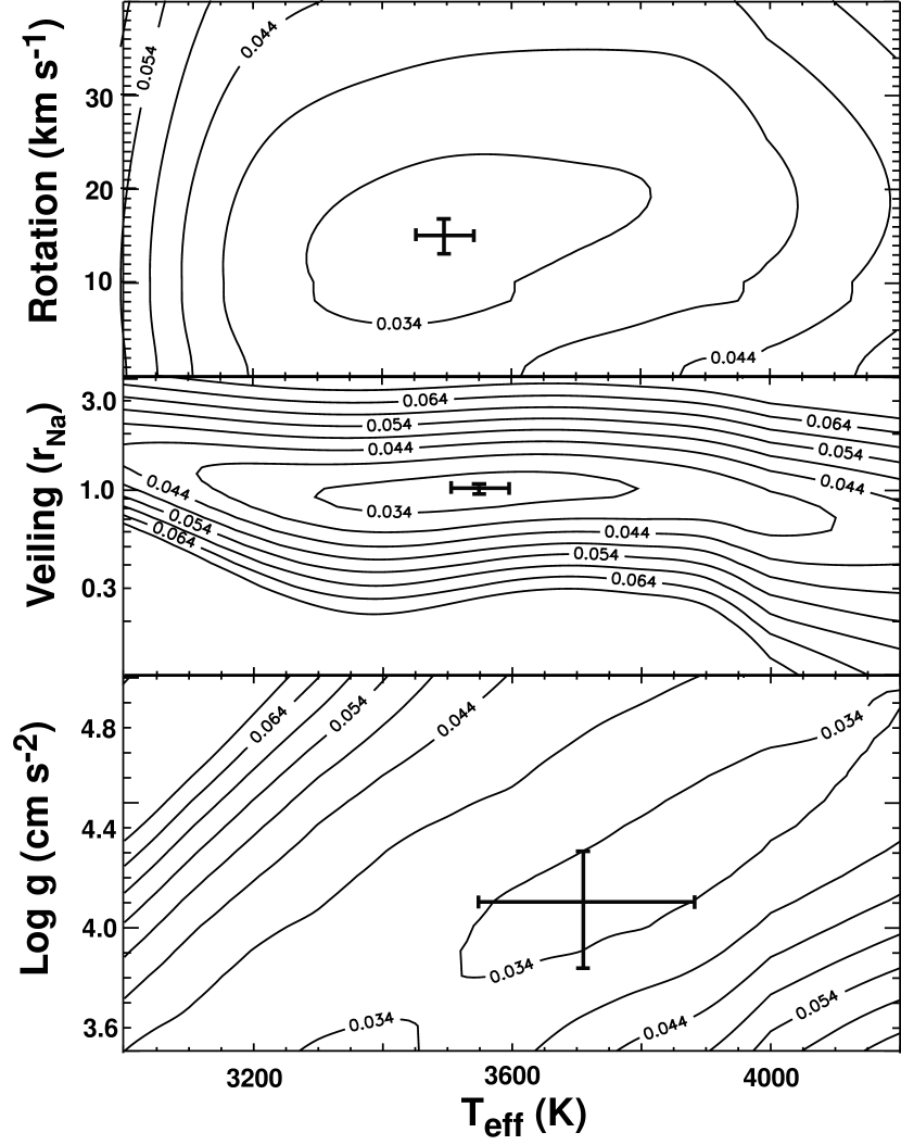
Figure 4: Variations of the RMS error in the T_eff–$v\sin i$, T_eff–r_Na, and T_eff–$\log g$ planes for a comparision of the noisy artificial spectrum from Figure 3 (where fluxes are normalized to one) to noiseless synthetic spectra. The contours show the RMS deviation of the noisy spectrum from the model at each point in the parameter space. We produced each two–parameter plot while holding the other two variables fixed at the values matching the correct values for the target spectrum. The error bar at the RMS minimum in each plot represents the standard deviation of the best fit value for S/N = 30 spectra with different noise seeds.

We illustrate the minimization process in Figure 4 which shows the variation of the RMS difference between an artificial noisy spectrum and various synthesis models of the Na interval as a function of the search parameters. We show variations of $\log g$ even though we would normally fix this parameter at a best–guess value when only Na interval data are available. The figure displays the RMS difference and thereby the shape of the minimum in the T_eff–$v\sin i$ plane, the T_eff–r_Na plane, and the T_eff–$\log g$ plane as the two variables are varied while the other two variables are held fixed at their nominal values. In all three planes, there are well–determined minima in the fits to the spectrum of the Na interval for all variables except $\log g$. The minimum in the T_eff–$\log g$ plane is very shallow. It is the one plane where we do not usually recover the input model. The grid in the $\log g$ direction is fairly coarse ($\Delta\log g=0.5$) and some noise seeds for the artificial spectrum at $\log g=4.0$ even find the lowest RMS value at the edge of the grid ($\log g=3.5$), leaving the exact location of the minimum uncertain. This cut (see bottom panel of Figure 4) illustrates that an incorrect guess of $\log g$ for real target spectra can lead to systematic errors in the derived value of T_eff (see $\S$ 4).

3.2.2 Solving Simultaneously for T_eff and $\log g$

There is a strong inverse dependence of the (2–0) ¹²CO bandhead equivalent width on $\log g$. There is also a weaker but noticeable dependence of the line equivalent width for the Na interval with $\log g$. Figure 5 plots the ratio of (2–0) ¹²CO to Na interval photospheric equivalent width (the equivalent width summed over the lines within the interval after removal of any non–photospheric continuum from the spectrum (see Appendix A) as a function of T_eff for $\log g$ values ranging from 3.5 to 5.0. We derived this ratio from the NextGen photospheric models by creating synthetic spectra for the relevant intervals and integrating the spectra over the bands marked in Figure 1. For T${}_{\rm eff}>$ 3700 K, the ratio varies strongly with $\log g$ and is almost independent of temperature. For lower temperatures, the ratio still varies strongly with $\log g$ but T_eff must also be known to correct for the sensitivity of the equivalent width ratio to temperature.

In $\S$ 3.2.1, we derived T_eff, $v\sin i$, and r_Na from spectra of the Na interval while holding $\log g$ fixed. When we have data available for both the Na and the ¹²CO intervals, we are able to solve for $\log g$ rather than just assume its value. We determine $\log g$ and the other parameters iteratively. We begin by assuming $\log g=3.5$ and derive a best fit for T_eff, r_Na, and $v\sin i$ using the Na observations as in $\S$ 3.2.1. We take the values of T_eff and r_Na that this process produces and use them, together with the integrals over the spectral intervals shown in Figure 1, to compute the ratio of photospheric equivalent widths in the ¹²CO and Na intervals (see Appendix A). With the photospheric equivalent width ratio and the derived value of T_eff, we can use the relations plotted in Figure 5 to estimate $\log g$ and use this new value of $\log g$ in an iteration of the procedure for deriving T_eff, $v\sin i$ and r_Na from the observed spectrum of the Na interval. The iterative procedure converges quickly on a value for $\log g$. The first two panels of Figure 6 illustrate how the derivation of parameters from the Na interval plus the use of the ¹²CO interval photospheric equivalent width work together to produce the correct value for all four parameters. The figure shows how the equivalent width of the CO bandhead varies significantly more than the equivalent width of the Na interval going from (T_eff, $\log g$) = (3600 K, 3.5) to (4000 K, 4.5). Note that at low temperatures and high surface gravities, the Na line wings extend beyond the spectral interval over which we compute the equivalent width for the Na interval. When the data cover a similar or narrower spectral interval, observations of cool and/or high surface gravity stars must be corrected for the fact that the intensity at the edges of the band is not fully at the level of the photospheric continuum. We have applied this correction in Figure 5. Therefore even when data with broader spectral coverage are available, the measured equivalent width should be computed only over the marked intervals in Figure 1 for comparison to Figure 5.

Although our procedure for using the CO interval together with the Na interval to determine $\log g$ does not, in principle, require high spectral resolution observations of the CO bandhead, such observations are very useful. In the youngest YSOs, the excess non–photospheric emission can be many times greater than the emission from the photosphere itself. In such cases, the equivalent widths of the lines not only fail to represent the conditions in the stellar atmosphere but also can be extremely hard to measure. In low resolution spectra, the combination of dilution by non–photospheric emission and dilution because the features are unresolved can make reliable measures of equivalent widths very problematic. Good atmospheric cancellation is also difficult because of the inherent messiness both of the stellar and the telluric spectrum in the region of the (2–0) ¹²CO bandhead. Higher resolution spectra improve the situation because they make it easier to cancel telluric lines and because line–to–continuum ratios are larger.

At high resolution, where we can resolve the CO bandhead and also the adjacent features in the ascending and descending R–branch and where effective telluric line cancellation is possible, we can match the depth and shape of a CO bandhead to obtain useful information about both T_eff and $\log g$ that does not depend strongly on precise determination of the continuum level.

The third panel in Figure 6 illustrates the dependence of the spectral shape in the (2–0) ¹²CO bandhead on $\log g$ and T_eff as it would be seen at high spectral resolution. This panel demonstrates the potential for using detailed spectral shapes in the ¹²CO interval to improve the robustness of the stellar parameter derivation scheme. It shows the difference between the synthetic spectrum for the CO interval for (T_eff, $\log g$)=(3800 K, 4.0) and (4000 K, 4.5) and (3600 K, 3.5). We see that, in addition to the equivalent width changes, there is a change in the individual line depths and in the shape of the envelope of the bandhead at this resolving power (R $=50,000$). In the current work, however, we restrict ourselves to analyzing the results of detailed spectral synthesis matching for the Na interval combined with use of the Na/¹²CO photospheric equivalent width ratio to arrive at accurate values for T_eff, $v\sin i$, r_Na and $\log g$.

4 Analysis of Errors

Now that we have developed a procedure for determining stellar parameters from high resolution spectra, we would like to know how well it works, both the sensitivity of the fitting routine and the uniqueness of the derived solutions. We discuss here four classes of uncertainty: (1) The sensitivity of the model fitting to random noise in the spectra. (2) Internal systematic uncertainties arising from the optimization scheme and from degeneracies between various stellar parameters. (3) External systematic errors introduced by transformations from one theoretical framework to another. (4) Errors arising from non–random effects present in the data. We evaluate the effects of these problems on derived parameters using simulations, real data, and modifications of real data. We first analyze the errors in parameters derived using only the Na interval and then discuss changes in these errors and the uncertainty in the determination of $\log g$ when observations of both the Na and ¹²CO intervals are available.

4.1 Random Errors

A generalized assessment of the sensitivity of our fitting routines to random errors is not possible. The sensitivity of the T_eff, $v\sin i$, and r_Na determinations will be not only a function of the signal–to–noise ratio (S/N) of the spectra but also will depend on the widths of the lines and on their strengths relative to the continuum (that is, effectively on all four parameters). By working with a typical spectrum, however, we can get a rough idea of what S/N we require to reach the point where random noise in the spectra no longer dominates the uncertainty in determining stellar parameters. We illustrate the sensitivity to random errors by taking a synthetic spectrum for the model shown in Figure 1a and adding more and more Gaussian random noise to it. We take each artificially noisy spectrum, find the best–fit values for T_eff, $v\sin i$ and r_Na in the usual way, by calculating the RMS difference between this spectrum and a set of noise–free synthesis models covering a range in all three parameters and then interpolating to obtain the best–fit values. At each S/N level, we re–seed the noisy spectrum 30 times and repeat the fitting procedure. The standard deviation about the mean value of each derived parameter for this ensemble of noisy spectra then reflects the uncertainty due to random noise at a given S/N level. Figure 7 shows how the standard deviation about the mean derived T_eff, $v\sin i$, and r_Na varies for noisy versions of the Na interval spectrum in Figure 1a (with continuum added to make r${}_{\rm Na}=1$) as the S/N decreases. For this particular case, the uncertainty in the T_eff due to random errors is less than 100 K for S/N $>$ 50. Random errors result in uncertainties of less than one spectral subclass as soon as the S/N ratio is greater than 35 at R $=50,000$. At S/N = 50, the random uncertainty in $v\sin i$ is 2 km s^-1 and that in r_Na is 0.13. The curves shown in Figure 7 illustrate the behavior of the random errors with S/N for a spectrum with r_Na=1. For sources with other values of r_Na, we can derive the S/N required for a given uncertainty in T_eff, $v\sin i$, or (1+r_Na) by multiplying the value shown in Figure 7 by (1+r_Na)/2. For a given uncertainty in (1+r_Na), the uncertainty in r_Na itself is (1+r_Na) times larger. Once the S/N exceeds $\sim$35$\times$(1+r_Na), other forms of errors begin to dominate the uncertainty in the derivation of stellar parameters from the K–band spectral fitting technique.

For $v\sin i$, we also tested the dependence of the uncertainty on T_eff. We used models with stellar rotation (25 km s^-1), instrumental smoothing (R $=50,000$) and Gaussian noise (S/N $=30$ per R $=240,000$ channel with r_Na=0) added to simulate real data. We fit the modified synthetic spectra to a set of noiseless models keeping the temperature fixed at the correct value and allowing the RMS minimization algorithm to select the best $v\sin i$ value. This was repeated with 30 noise seeds for each temperature giving a mean and 1 $\sigma$ error for $v\sin i$ for temperatures between 3200 K and 4400 K. The 1$\sigma$ error is less than 2 km s^-1 over the entire temperature range.

4.2 Uncertainties Arising from Internal Systematics

For some pairs of stellar parameters, changes of both parameters simultaneously in a certain sense can keep the line shapes and depths almost unchanged. These partial degeneracies in the output line shapes between different groupings of stellar parameters can have the effect of exaggerating the uncertainties caused by random errors. For minimizations of model–observed spectral differences in the Na interval, this effect is most evident in the broadness of the minimum RMS error along a diagonal in the T${}_{\rm eff}-\log g$ plane (Figure 4, bottom). When the spectra are noisy or imperfect, there is a range of temperature–gravity pairs with very similar RMS values. Similar degeneracies for other lines in the near–IR have caused difficulties when attempting to type YSOs from low resolution near–IR spectra, unless one knows what luminosity class is appropriate for the template stars (Luhman & Rieke, 1999).

The similar line shapes for models along a diagonal in the temperature–gravity plane mean that we can introduce systematic errors in the derived T_eff when we assume a value of $\log g$ and then derive the temperature. We can illustrate and assess this effect with fits to models. Figure 8 summarizes the results of our tests by showing how the derived temperatures deviate from the target spectrum temperature at different target values of T_eff. Typically, our best fits for T_eff using models with a $\log g$ differing by $\pm 0.5$ from the $\log g$ of the target spectra mis–estimate the temperature by about 7%. This difference is approximately 1–2 spectral subclasses over the range of T_eff relevant to our study. If we later obtain an independent estimate of $\log g$, we can correct the derived T_eff. For data where we derive an effective temperature from the Na interval assuming some value of $\log g$, we can correct the derived $\log$ T_eff by $+$0.06 for every $\log g=1$ difference between the assumed and the correct values. Making this correction, we recover the actual value of T_eff to within better than 4%.

The way in which we create the error space from comparisons of observed target spectra and synthesized model spectra may have a systematic effect on the derived parameters. The error space shown in Figure 4 represents the RMS deviation of the target spectrum from the models over selected intervals where line absorption was present (see Figure 3). This scheme allows for variations of feature depths and shapes. Because it is a straight RMS, it weights the stronger features, in particular the Na features, more heavily. One might ask if this is the best scheme, i.e. does it make the uncertainties in the derived parameters larger than they need to be? In its favor is the ability of the Na line depths to distinguish the value of r_Na and the sensitivity of the depth and shape of these lines to T_eff and $\log g$. On the other side of the ledger is the low weight a straight RMS gives to the weaker Sc and Si lines. The ratio of these lines is the most sensitive temperature indicator in the Na interval. More complex schemes that make better use of the information content of the weaker lines and the subtleties of the line shapes are certainly possible. When the S/N gets large enough that systematic errors dominate over random errors, a straight RMS does not do as well as a weighted error scheme, but remains a reasonable approximation. The simple RMS scheme, however, has the great advantage that it finds the right parameters robustly over our whole temperature range at various values of r_Na and $v\sin i$ and that its level of complexity is appropriate to S/N ratios of 30–50 where random errors are just beginning to give way to systematics.

4.3 Errors in the Radial Velocity Determination

When we work with real data, we use the RMS minimization of the difference between the data and the synthesis models to determine the best radial velocity shift of the observed stars along with the best–fit stellar parameters. A narrow search range in radial velocity space is first selected by inspection. The data and models are interpolated to a higher dispersion (R${}_{\rm pix}=360,000$). We then use the minimum RMS of the residuals to the fit to select the best sub–pixel radial velocity shift. Tests with artificial spectra show that random errors in the radial velocity determination due to noise in the spectrum are small ($<0.5$ km s^-1) for spectra with S/N $>$ 30 per pixel (R${}_{\rm pix}=240,000$).

We also examined how errors in the radial velocity fit affect our determination of the stellar parameters. For a S/N $\sim$30 per pixel, noise in the spectra is a much more significant factor in causing errors in $v\sin i$ than the error in the radial velocity determination. Stellar parameters determined mostly from line depths (i.e. effective temperature and veiling), are not sensitive to radial velocity errors at the 5 km s^-1 level.

5 Comparison with Standards and External Systematics

We can use the spectra we have taken in the 2.2 $\mu$m Na interval of MK standard stars to perform a real–world test of our fitting technique. We discuss here the test results for T_eff and $v\sin i$. We also add an artificial infrared excess and rotation velocity to the MK standards in order to look for systematic effects in the determination of r_Na and refine our understanding of such effects on our determination of $v\sin i$.

The high resolution spectra we use to derive stellar parameters are imperfect representations of the source spectra. Systematic problems with the data include imperfect flat–fielding, defects in the cancellation of telluric features and the presence of scattered light or leaked out–of–order stellar radiation. The use of high resolution spectra in our analysis reduces the effect of these problems substantially. By choosing restricted wavelength intervals over which to match the synthetic models to the data, we minimize flat–fielding effects since mismatches in the shapes of the synthetic and observed lines then play a bigger role in influencing the RMS difference. At high spectral resolution, the residuals of telluric lines cover a limited and known part of wavelength space. We simply exclude these regions from our fitting spectral matching intervals. Scattered light is usually removed in the data analysis if the source and sky have been switched regularly between two positions along the slit.

The continuum level for our spectra could be another free parameter in our spectral fitting routine, though we have chosen to leave the continuum fixed when finding the minimum RMS difference between the target and synthetic spectra. For our target spectra, we have normalized the continuum based on a linear fit of two points close to the edges of the spectrum and farthest from Na I lines where the potential influence by any damping wings is minimized. In some cases where the instantaneous spectral coverage of the spectrometer is limited, it can be difficult to set the continuum level in the spectra correctly, particularly for the cooler stars and stars with higher surface gravities where the wings of the Na lines are extended.

Differences between the effective temperatures derived from optical spectral types and the T_eff values we derive from high resolution observations of the Na interval reflect the sum of the internal errors in our determination of T_eff, errors in spectral typing from optical observations, and errors in converting from spectral types to effective temperatures. This last error can be substantial. De Jager & Nieuwenhuijzen (1987) estimate errors of 0.021 in the $\log$ of T_eff in their spectral type–T_eff conversion for dwarfs, corresponding to $\pm$200 K at T_eff=4000 K.

Table 1 lists the effective temperature we derive for MK standards in our sample using the Na interval, as well as temperatures derived from the optical spectral types using the T_eff–spectral type relation of de Jager & Nieuwenhuijzen (1987). In Figure 9, we plot the near–IR T_eff against T_eff determined from optical measurements by a variety of different techniques. For a given target, the spread of different symbols along the horizontal axis illustrates differences in the conversion between spectral type and temperature (de Jager & Nieuwenhuijzen, 1987; Ali et al., 1995; Alonso et al., 1996; Allen, 2000). The figure also includes temperatures derived using observed B–V colors and the conversion relation of Kenyon & Hartmann (1995) which we will also apply to YSOs. The vertical error bars (placed on the de Jager T_eff points) show our estimate of the 1$\sigma$ uncertainty due to random noise in our data. The errors for our T_eff determinations were derived by carrying out an analysis similar to that used to create Figure 7 but at the temperature and S/N ratio appropriate to each MK standard. The size of these errors indicates that systematic effects must dominate any differences between the optical and infrared results.

For the luminosity class V MK standards, a best fit to the T_eff (optical, de Jager & Nieuwenhuijzen, 1987) versus T_eff(Na interval) yields:

$${\rm T_{eff}(Na)}=1.08\times{\rm T_{eff}}(\rm{de~{}Jager})-295$$ (1)

The 1$\sigma$ deviation from this relation is 113 K. For the same sources, the 1$\sigma$ deviation for an “assumed” relation of T_eff(Na)=T_eff(de Jager) is 141 K, which is still less than the quoted uncertainty in the spectral type–temperature conversion.

All of the MK standards in our sample are fairly slow rotators and therefore not particularly useful for tests of the accuracy of our fits to the Na interval for $v\sin i$. Table 1 lists the values of $v\sin i$ from optical spectra as well as the results of our fit to the Na interval. For these near–IR results, we have removed the effect of slit broadening by subtracting it in quadrature from the fitted value to produce the intrinsic widths or upper limits listed in the Table. For 10 of the 11 stars, the optical and near–IR measurements and upper limits are consistent with each other. For the one discrepant source, HD 131976, where we measure $v\sin i$= 10 km s^-1, versus the value of 1.4 km s^-1 measured by Duquennoy & Mayor (1988), the S/N for the infrared measurement is lower than that of any other standard in our sample.

When we study a particular embedded PMS star, we usually do not know its metallicity. Assuming solar metallicity, however, should not cause problems for comparisons between models and stellar spectra since the deviations from solar metallicity are usually quite small, typically $\Delta$[Fe/H] $<$ 0.1 (Padgett, 1996). For the MK standards in the field, differences between the assumed and actual stellar abundance can cause systematic differences in the T_eff scale. Eight of the MK standards we have observed as a test sample have measured abundances ranging from +0.02 dex above solar to $-$0.30 dex below (Table A Spectroscopic Technique for Measuring Stellar Properties of Pre–Main Sequence Stars). For the comparison with MK standards in Figure 9, we fixed r_Na=0 and used the metallicities listed in Table A Spectroscopic Technique for Measuring Stellar Properties of Pre–Main Sequence Stars or solar metallicities when no measurements were available. For MK standards with measured non–solar metallicities, we computed separate grids of synthetic spectra for comparison with the observed spectra. Since the stellar atmosphere models available to us were gridded rather coarsely in metallicity for our purposes (every 0.5 dex), we constructed the spectral synthesis grids for mildly metal–poor stars ($0.3\leq[{\rm Fe/H}]\leq 0$) using solar metallicity model atmospheres but synthesizing the spectra using abundances scaled down by [Fe/H]. This procedure does not account perfectly for metallicity effects. If we constrain the search grid to a fixed veiling (r${}_{\rm Na}=0$) and metallicity determined from the literature, however, the best fit model (as determined by the minimum RMS difference) has a noticeably non–zero residual equivalent width when compared to the observed spectrum of the MK standard.

In order to test the ability of our fitting routine to derive $v\sin i$ and r_Na as well as T_eff from data containing realistic amounts of systematic deviation from ideal spectra, we have altered our PHOENIX observations of MK standards ($\S$ 2). We began with MK standards with very small rotation velocities ($v\sin i\leq 10$ km s^-1). These stars also had no intrinsic veiling (r_Na=0). As we showed above, if we hold r_Na fixed at zero, we recover the T_eff derived from optical spectra from our near–IR observations. To each spectrum, we then added a known amount of rotation ($v\sin i$ = 25 km s^-1) and veiling (tripling the amount of continuum to make r_Na = 2.0). The Na interval spectra of these doctored stars were then analyzed using our standard procedure. For 6 of the 7 objects, we recovered effective temperatures close to those derived from the unaltered stellar spectra, typically within one spectral subclass of the best–fit temperature for the unaltered spectrum (Table 2). The recovered temperature tended, however, to be systematically lower than the values derived holding r_Na fixed and the recovered r_Na values were higher than those we put into the spectra. The seventh object, HD 117176, has a T_eff higher than the range for which the technique is fully reliable. For this source, the fitting routine derived a lower temperature and higher veiling. In all cases, the recovered $v\sin i$ was greater than or equal to but always within 5 km s^-1 of the 25 km s^-1 we put into the spectra.

Table 2 also lists the values of r_Na derived for the MK standards to which we had artificially added an r_Na=2.0. As in the case of T_eff, the fit for HD 117176 differs strongly from the input value. For the remaining luminosity class V sources, the derived r_Na is 2.7 $\pm$0.22. For the two luminosity class IV sources, the average value is 2.4. One possible contributor to this systematic difference may be the damping parameter used in the line synthesis. The parameter that works for the solar spectrum may not be ideal for the cooler target stars. For the YSOs, whose gravities are more comparable to the luminosity class IV MK standards, this systematic problem may lead to an overestimate of r_Na by $\Delta$r_Na= 0.13$\times$(1+ r_Na). Differences between the value of r_Na derived from analysis of the Na interval spectra and values derived by other methods that are smaller than this $\Delta$r_Na are probably not significant. Further analysis with a better sample of MK standards will be needed to understand this effect more fully.

On a real sample of PMS stars, one would be forced to address the effects of possible binary companions. Close companions will be recognizable in high resolution spectra because of their effect on stellar radial velocities. Beyond a few AU, the radial velocity effects will be much less apparent and imaging will be needed. A recent compilation of multiplicity data yields a companion star frequency for TTSs in nearby star forming regions of 24% $\pm$11% (Ophiuchus) and 37% $\pm$9% (Taurus), (Barsony, Koresko, & Matthews, 2003), for bright companions ($\Delta$K $\leq$ 2–3 mag). Of these, 40% have large enough separations to make them readily separable for direct imaging or spectroscopy. Therefore, $\sim$20% of a sample of stars in nearby star forming regions will have spectra that suffer from contamination of a secondary component. Spectroscopy using adaptive optics will eliminate this problem for the vast majority of sources.

Continuum opacity due to molecules not present in our synthesis models is also a likely contributor to the systematic difference in the derived veiling values. Preliminary tests with numerous CO, SiO, OH, and H₂O lines that blanket the Na interval reveal a $\sim$5% decrease in the continuum compared to the continuum determined from our synthesis models (Carbon 2003, private communication). Neglecting this decrease in the continuum relative to the cores of the photospheric lines could cause overestimates in the derived veiling by $\sim$0.05, as well as slightly altering the shapes of the atomic line wings.

6 Conclusions

We have described, demonstrated and evaluated a technique for deriving effective temperatures, surface gravities, rotation rates, and infrared excesses from high resolution spectra of PMS stars in the near–IR. In a companion paper (DJW03), we use this technique to study a sample of YSOs in the $\rho$ Ophiuchi molecular cloud core. Using the Na interval at 2.2 $\mu$m, we can recover the effective temperatures of dwarf MK standards at a level below the uncertainty in the spectral type–temperature conversion. The spectra also give us a good measure of the rotation velocity and continuum veiling. With the addition of a measurement of the relative flux between the (2–0) ¹²CO bandhead and the Na interval, it is possible to determine the surface gravity of YSOs and to remove uncertainties in the temperature caused by a partial degeneracy with $\log g$. The derived parameters are insensitive to extinction along the line–of–sight and need photometric information only to tie together the intensity scales in non–contiguous high resolution spectra and to correct for differential reddening between 2.2 $\mu$m and 2.3 $\mu$m.

It is clear from the results that the ability to work with weak features and to measure line shapes as well as equivalent widths can make high resolution near–IR spectroscopy a valuable tool for studies of highly obscured stars and of young objects with strong excess infrared emission. The technique we develop here is robust enough to deal with sources with a range of different S/N ratios and with excess near–IR emission.

In the future, it will be worthwhile to investigate whether high resolution spectra of other near–IR intervals could add useful information about the stellar parameters. We would also like to investigate more sophisticated matching routines that might make better use of the sensitivity of individual weak features to various stellar parameters. For studies of cooler, lower mass YSOs, it would be useful to produce models and line syntheses for lower temperature objects.

Appendix A Surface Gravity Diagnostics

The ratio of photospheric equivalent widths from the Na doublet at 2.2 $\mu$m and the (2–0) ¹²CO bandhead at 2.3 $\mu$m is sensitive to changes in surface gravity. Figure 5 shows that this ratio gives a good estimate of $\log g$ across the entire range in effective temperature and surface gravity relevant to the study of low mass PMS stars. In that figure, the photospheric equivalent widths in both the Na interval and the ¹²CO interval were calculated from model spectra synthesized from the NextGen stellar atmosphere models for $\log g=3.5$–5.0 and T${}_{\rm eff}=3000$–5000 K.

The problem in studying YSOs is that they suffer both from significant extinction and reddening and often from the presence of excess continuum emission that can be larger than the emission from the photospheres themselves. As a result, the measured equivalent width ratios do not accurately reflect the ratio of photospheric equivalent widths that would be relevant for comparison with Figure 5. What we would like to be able to do is to take the observed equivalent widths and, using as little additional data as possible and in a way as insensitive as possible to the effects of reddening and infrared excess, correct the observed equivalent width ratio to the photospheric equivalent width ratio. We outline here a procedure that uses near–IR photometry to correct for differential reddening between 2.2 $\mu$m and 2.3 $\mu$m and low resolution spectroscopic data (if necessary) to correct for throughput differences between the high resolution spectra in the Na and ¹²CO intervals. In both cases, the corrections are usually quite small. To make it easier to use the equivalent width ratio as a diagnostic for surface gravity, the expressions below are geared to observable quantities.

Starting with an absorption spectrum at high resolution, we define the measured equivalent width (MEW) in terms of the measured flux ($F_{\lambda}$) relative to the measured continuum ($c_{\lambda}$):

$${\rm MEW}=\int{\frac{c_{\lambda}-F_{\lambda}}{c_{\lambda}}}\,d\lambda$$ (A1)

We define the photospheric equivalent width (PEW) to be the equivalent width of a photospheric absorption line without its value being altered by the presence of continuum veiling originating outside of the photosphere (r_λ=(F_source – F_phot)/F_phot). We define, then, photospheric equivalent widths for the regions around the Na features at 2.2 $\mu$m (PEW_Na) and the shortest wavelength part of the (2–0) ¹²CO R–branch at 2.3 $\mu$m (PEW_CO).

$${\rm PEW}_{\rm Na}=\int_{2.202\mu\rm m}^{2.212\mu\rm m}\frac{c_{2.2\mu\rm m}-F(\lambda)}{c_{2.2\mu\rm m}}(1+r_{2.2\mu\rm m})\,d\lambda$$ (A2)

$${\rm PEW}_{\rm CO}=\int_{2.2925\mu\rm m}^{2.3000\mu\rm m}\frac{c_{2.3\mu\rm m}-F(\lambda)}{c_{2.3\mu\rm m}}(1+r_{2.3\mu\rm m})\,d\lambda$$ (A3)

The photospheric continuum $p_{\lambda}$ is altered by infrared excess (increasing the continuum by a factor ($1+r_{\lambda}$)), probably due to thermal emission from a warm surrounding disk, and extinction ($A_{\lambda}$) along the line–of–sight. The corresponding expressions for the measured continuum ($c_{\lambda}$) in the two wavelength regions of interest are:

$$c_{2.2\mu\rm m}=p_{2.2\mu\rm m}(1+r_{2.2\mu\rm m})10^{-0.4A_{2.2\mu\rm m}}~{}~{}{\rm erg}~{}{\rm s}^{-1}~{}{\rm cm}^{-2}~{}\mu\rm m^{-1}$$ (A4)

$$c_{2.3\mu\rm m}=p_{2.3\mu\rm m}(1+r_{2.3\mu\rm m})10^{-0.4A_{2.3\mu\rm m}}~{}~{}\rm erg~{}s^{-1}~{}cm^{-2}~{}\mu m^{-1}$$ (A5)

Knowing the effective temperature (T_eff) allows us to relate the photospheric continua to each other by assuming a blackbody dependence ($B(T,\lambda)$).

$$\chi(T_{\rm eff})=\frac{p_{2.3\mu\rm m}}{p_{2.2\mu\rm m}}=\frac{B_{\lambda}(T_{\rm eff},2.3\mu\rm m)}{B_{\lambda}(T_{\rm eff},2.2\mu\rm m)}$$ (A6)

By taking the ratio of equations A4 & A5 and substitution of equation A6, we arrive at an expression for a quantity we can measure with low resolution spectra or with cross dispersed high resolution spectra covering the full range of the two wavelength intervals: the ratio of measured continua at two different wavelengths.

$$\frac{c_{2.2\mu\rm m}}{c_{2.3\mu\rm m}}=\frac{(1+r_{2.2\mu\rm m})10^{-0.4A_{2.2\mu\rm m}}}{\chi(T_{\rm eff})(1+r_{2.3\mu\rm m})10^{-0.4A_{2.3\mu\rm m}}}$$ (A7)

Re–arranging equation A7 and substituting into the ratio of equations A2 & A3 removes the dependence on any continuum veiling:

$$\frac{{\rm PEW}_{\rm Na}}{{\rm PEW}_{\rm CO}}=\frac{{\rm MEW}_{\rm Na}}{{\rm MEW}_{\rm CO}}\frac{c_{2.2\mu\rm m}}{c_{2.3\mu\rm m}}\chi(T_{\rm eff})10^{-0.4(A_{2.3\mu\rm m}-A_{2.2\mu\rm m})}$$ (A8)

This expression provides terms on the right hand side that we can measure with spectroscopy and photometry allowing us to utilize the surface gravity dependence on photospheric equivalent ratios in models as illustrated in Figure 5.

Figure 1: The intervals within the 2.0–2.4 $\mu$m K window used for spectral synthesis analysis of high resolution data. The spectra are from a synthesis of a T${}_{\rm eff}=4000$ K, $\log g=3.5$ NextGen atmosphere model (Hauschildt et al., 1999), assuming a resolving power $\lambda$/$\Delta\lambda=50,000$. The intensity is normalized to the photospheric continuum. The Na interval shows the numerous neutral atomic species present in the photospheres of cool stars (top). The ¹²CO interval shows the bandhead and the v=2–0 R–branch transitions of ¹²CO (bottom). The vertical lines show the boundaries for the intervals used to compute the equivalent width ratios plotted in Figure 5.

Figure 2: A grid of spectral syntheses based on NextGen (Hauschildt et al., 1999) atmosphere models. These spectra illustrate the change in Na line shape and depth and the variations in Si/Sc for temperatures from 3300 K to 4200 K for $\log g$ fixed at 4.0. Spectra have been smoothed to a R = 50,000.

Figure 3: Fits to a noisy artificial spectrum of the Na interval. The thin solid line shows an artificial spectrum for T${}_{\rm eff}=3600$ K, $\log g=4.0$, $v\sin i=15$ km s^-1, and r${}_{\rm Na}=1.0$. We have smoothed this spectrum to R = 50,000 and added Gaussian random noise to the spectrum to produce a S/N = 30 (per pixel with R = 240,000 pixels). Overlaid on each of the 3 panels is a noiseless synthetic spectrum (bold lines) for $\log g=4.0$, T${}_{\rm eff}=4000$K (top), T${}_{\rm eff}=3600$K (middle), and T${}_{\rm eff}=3200$K (bottom). In each panel, the best fit was found holding T_eff fixed at the listed value but allowing r_Na and $v\sin i$ to vary. The difference between the noisy artificial and noiseless spectra is displayed at the bottom of each panel. The vertical dashed lines are the subintervals chosen in this case to enclose regions with significant line flux over which we will compute the RMS difference between the noisy artificial spectrum and the grid of noiseless synthetic spectra. In the lower left of each panel is the RMS difference between the noisy and noiseless spectrum normalized to the number of points in the two subintervals that enclose the photospheric lines.

Figure 5: The ratio of CO interval equivalent width to Na interval equivalent width as a function of temperature, plotted for surfaces gravities between $\log g=3.5$ and $\log g=5.0$. Equivalent widths were computed over the Na and ¹²CO intervals as defined in Figure 1. The relatively flat shape of these isogravity lines with temperature illustrates the value of the ¹²CO/Na line flux ratio as a good diagnostic of surface gravity.

Figure 6: Demonstration of simultaneous derivation of T_eff and $\log g$. The top panel shows a S/N = 50 synthetic spectrum for (T_eff, $\log g$)= (3800K, 4.0). Below that we show differences between this spectrum and models for (T${}_{\rm eff},\log g)=$ (3500K, 3.5), (3800K, 4.0), and (4000K, 4.5) illustrating the effects of the broad minimum in the errors as T_eff and $\log g$ increase simultaneously. The middle panel shows the difference between the equivalent width of the Na and CO interval for these (T${}_{\rm eff},\log g)$ pairs and (T${}_{\rm eff},\log g)=$ (3800K, 4.0), normalized to the equivalent width of the (3800K, 4.0) spectrum. The bottom panel shows the associated strong variations in the spectra of the CO interval.

Figure 7: Standard deviation of the derived value of T_eff (derived using the Na interval only) as a function of S/N. To construct this plot, we used a noisy artificial spectrum with T_eff=4200K, $\log g$=4.0, $v\sin i$=15 kms^-1, and r_Na=1.0 as the target and fit for the best temperature allowing all parameters except $\log g$ to vary. We compared the target and model spectra at sampling points spaced every $\Delta\lambda$/$\lambda$=(1/240,000) along spectra smoothed to a resolving power of 50,000. The S/N is that appropriate to data binned to channels $\Delta\lambda$/$\lambda$=(1/50,000) wide.

Figure 8: The effect on the best–fit value of T_eff of assuming an incorrect value for $\log g$. At each temperature, a synthetic target spectrum with $\log g$=4.0 and two grids of MOOG models with $\log g$=3.5 and $\log g$=4.5 were created. We then fit for the temperature of the target spectrum using each of the grids with the different values of $\log g$. The solid lines show the difference between the logarithm of the best–fit T_eff to the target spectrum derived by using the $\log g$=3.5 (bottom) or 4.5 (top) grids and the logarithm of the target spectrum T_eff.

Figure 9: Test of our effective temperature determinations (vertical axis) against temperature determinations available in the literature for MK standards (horizontal axis). The small vertical error bars represent $\pm$1$\sigma$ uncertainties due to the noise in the observed spectra, determined by calculations similar to those used in Figure 7 at each temperature and at a S/N comparable to that of the data. The horizontal error bar in the lower right corner of the Figure shows the 1 $\sigma$ uncertainty in the spectral type to T_eff conversion at 4000 K (de Jager & Nieuwenhuijzen, 1987). We placed the symbols in the x direction by converting the spectral types (Table A Spectroscopic Technique for Measuring Stellar Properties of Pre–Main Sequence Stars) to T_eff using various spectral type–T_eff relations: open circles (Alonso et al., 1996), open triangles (Ali et al., 1995), open squares (Allen, 2000) vertical error bars (de Jager & Nieuwenhuijzen, 1987). Unless otherwise marked, all sources are dwarfs, luminosity class V. The open pentagons show the T_eff derived from the reported B–V colors using the conversion relation of Kenyon & Hartmann (1995). The dashed line shows the relation T_eff(near–IR) = T_eff(optical).

Table 1: Observed MK standards

Standard	Spectral	Optical	Near–IR	Optical	Near–IR	Metal-	S/N
Star	Type	$T_{\rm eff}$	$T_{\rm eff}$	$v\sin i$	$v\sin i$	licity
		(K)	(K)	(km s${}^{-1})$	(km s${}^{-1})$	[Fe/H]
HD 117176	G4V	5636	5980	10	$<$3	$-$0.11	120
HR 4496	G8V	5439	5400	$<$15	$<$9	$-$0.14	300
HR 4496	G8V	5439	5460	$<$15	$<$3	$-$0.14	110
HD 185144	K0V	5152	5260	$<$15	$<$3	$-$0.23	120
GL 28	K2V	4838	4880	2.5	$<$9	$-$0.05	180
HR 5568	K4V	4539	4580	$<$12	$<$9	0.016	170
GL 338A	M0V	3837	3660	2.9	$<$9	…	155
GL 338A	M0V	3837	3650	2.9	$<$3	…	110
HD 131976	M1.5V	3589	3610	1.4	10	…	75
GL 15A	M2V	3523	3630	$<$2.9	$<$9	…	150
GL 402	M4V	3289	3290	$<$2.3	$<$9	…	110
HD 188512	G8IV	5100	4700	1.8	$<$3	$-$0.30	130
HD 142091	K1IVa	4800	4680	1.9	$<$3	$-$0.04	100

References. — (1) Keenan & McNeil (1989) (2) Kirkpatrick et al. (1991) (3) Hearnshaw (1974b) (4) Hearnshaw (1974a) (5) McWilliam (1990) (6) Marsakov & Shevelev (1988) (7) Taylor (1995) (8)Glebocki & Stawikowski (2000) (9) Strassmeier et al. (2000) (10) Delfosse et al. (1998) (11) Duquennoy & Mayor (1988) (12) Vogt et al. (1983) (13) de Medeiros & Mayor (1999) (14) Fekel (1997)

Table 2: Recovered parameters with rotation ($v\sin i=25$ km s^-1) and veiling (r${}_{\rm Na}=2.0$) added to MK standards

MK	Best Fit	Recovered	Recovered	Recovered	RMS
Standard	Teff	Teff	$v\sin i$	Veiling
	(K)	(K)	(km s-1)	(rNa)
HD 117176	5980	5240	27.0	3.8	0.00271
HR 4496	5400	5230	29.0	2.6	0.00152
HD 185144	5240	5000	29.0	2.7	0.00189
GL 338A	3650	3765	25.0	3.0	0.00333
HD 131976	3610	3580	30.0	2.5	0.00244
HD 188512	4700	4620	30.0	2.3	0.00165
HD 142091	4680	4620	29.0	2.5	0.00209

References

- Ali et al. (1995) Ali, B., Carr, J.S., DePoy, D.L., Frogel, J.A., & Sellgren, K. 1995, AJ, 110, 2415
- Allen (2000) Allen, C. W. 2000, Allen’s Astrophyical Quantities (New York, Springer–Verlag)
- Alonso et al. (1996) Alonso, A., Arribas, S., & Martinez–Roger, C. 1996, A&A, 313, 873
- Baldwin et al. (1973) Baldwin, J.R., Frogel, J.A., & Persson, S.E. 1973, ApJ, 184, 427
- Baraffe et al. (1998) Baraffe, I., Chabrier, G., Allard, F., & Hauschildt, P. H. 1998, A&A, 337, 403
- Barsony et al. (1997) Barsony, M., Kenyon, S.J., Lada, E.A., & Teuben P.J. 1997, ApJS, 112, 109
- Barsony, Koresko, & Matthews (2003) Barsony, M., Koresko, C., & Matthews, K. 2003, ApJ, 591, 1064
- Bontemps et al. (2001) Bontemps, S. et al. 2001, A&A, 372, 173
- Casali & Matthews (1992) Casali, M. M. & Matthews, H. E. 1992, MNRAS, 258, 399
- Casali & Eiroa (1996) Casali, M. M. & Eiroa, C. 1996, A&A, 306, 427
- Comerón et al (1993) Comerón, F., Rieke, G. H., Burrows, A., & Rieke, M. J. 1993, ApJ, 416, 185
- D’Antona & Mazzitelli (1997) D’Antona, F. & Mazzitelli, I. 1997, Mem. Soc. Astron. Italiana, 68, 823
- Delfosse et al. (1998) Delfosse, X., Forveille, T., Perrier, C., & Mayor, M. 1998, A&A, 331, 581
- de Jager & Nieuwenhuijzen (1987) de Jager, C. & Nieuwenhuijzen, H. 1987, A&A, 177, 217
- de Medeiros & Mayor (1999) de Medeiros, J. R. & Mayor, M. 1999, VizieR Online Data Catalog, 413, 990433
- Doppmann et al. (2003) Doppmann, G.W., Jaffe, D.T., White, R.J. 2003 AJ, submitted (DJW03)
- Duquennoy & Mayor (1988) Duquennoy, A. & Mayor, M. 1988, A&A, 200, 135
- Duquennoy & Mayor (1991) Duquennoy, A. & Mayor, M. 1991, A&A, 248, 485
- Edvardsson et al. (1993) Edvardsson, B., Andersen, J., Gustafsson, B., Lambert, D. L., Nissen, P. E., & Tomkin, J. 1993, A&A, 275, 101
- Fekel (1997) Fekel, F.C. 1997, PASP, 109, 514
- Ghez et al. (1993) Ghez, A. M., Neugebauer, G., & Matthews, K. 1993, AJ, 106, 2005
- Glebocki & Stawikowski (2000) Glebocki, R. & Stawikowski, A. 2000, Acta Astronomica, 50, 509
- Goorvitch & Chackerian (1994) Goorvitch, D. & Chackerian, C. Jr. 1994, ApJS, 91, 483
- Gray (1992) Gray, D. F. 1992, The Observation and Analysis of Stellar Photospheres, (New York, Cambridge Univ. Press)
- Gray, Graham, & Hoyt (2001) Gray, R. O., Graham, P. W., & Hoyt, S. R. 2001, AJ, 121, 2159
- Greene & Young (1992) Greene, T.P., & Young, E.T. 1992, ApJ, 395, 516
- Greene et al. (1993) Greene, T. P., Tokunaga, A. T., Toomey, D. W., & Carr, J. B. 1993, Proc. SPIE, 1946, 313
- Greene et al. (1994) Greene, T. P., Wilking, B. A., André, P., Young, E. T., & Lada, C. J. 1994, ApJ, 434, 614
- Greene & Meyer (1995) Greene, T. P. & Meyer, M. R. 1995, ApJ, 450, 233
- Greene & Lada (1996) Greene, T. P. & Lada, C. J. 1996, AJ, 112, 2184
- Greene & Lada (1997) Greene, T. P. & Lada, C. J. 1997, ApJ, 114, 2157
- Greene & Lada (2000) Greene, T. P. & Lada, C. J. 2000, ApJ, 120, 430
- Greene & Lada (2002) Greene, T. P. & Lada, C. J. 2002, AJ, 124, 2185
- Gullbring et al. (2000) Gullbring, E., Calvet, N., Muzerolle, J., & Hartmann, L. 2000, ApJ, 544, 927
- Hatmann et al. (1991) Hartmann, L., Stauffer, J. R., Kenyon, S. J., & Jones, B. F. 1991, AJ, 101, 1050
- Hauschildt et al. (1999) Hauschildt P.H., Allard, F. & Baron, E. 1999, ApJ, 512, 377
- Hearnshaw (1974a) Hearnshaw, J. B. 1974, A&A, 34, 263
- Hearnshaw (1974b) Hearnshaw, J. B. 1974, A&A, 36, 191
- Hinkle et al. (1998) Hinkle, K. H., Cuberly, R. W., Gaughan, N. A., Heynssens, J. B., Joyce, R. R., Ridgway, S. T., Schmitt, P., & Simmons, J. E. 1998, Proc. SPIE, 3354, 810
- Huang (1961) Huang, S. 1961, ApJ, 134, 12
- Johns–Krull & Valenti (2001) Johns–Krull, C. M. & Valenti, J. A. 2001, ApJ, 561, 1060
- Keenan & McNeil (1989) Keenan, P. C. & McNeil, R. C. 1989, ApJS, 71, 245
- Kenyon & Hartmann (1995) Kenyon, S. J. & Hartmann, L. 1995, ApJS, 101, 117
- Kenyon et al. (1998) Kenyon, S. J., Brown, D. I., Tout, C. A., & Berlind, P. 1998, ApJ, 115, 2491
- Kirkpatrick et al. (1991) Kirkpatrick, J. D., Henry, T. J., & McCarthy, D. W. 1991, ApJS, 77, 417
- Kirkpatrick et al. (1993) Kirkpatrick, J.D., Kelly, D.M., Rieke, G.H., Liebert, J. Allard, F., & Wehrse, R. 1993, ApJ, 402, 643
- Kleinmann & Hall (1986) Kleinmann, S. G., & Hall, D. N. B. 1986, ApJS, 62, 501
- Kurucz (1994) Kurucz, R. L. 1994, Atomic Data for Opacity Calculations, Kurucz CD–ROM No. 1
- Lada (1987) Lada, C. J. 1987, IAU Symp. 115: Star Forming Regions, 115, 1
- Lancon & Rocca–Volmerange (1992) Lancon, A., & Rocca–Volmerange, B. 1992, A&AS, 96, 593
- Leggett et al. (1996) Leggett, S.K., Allard, F., Berriman, G., Dahn, C.C., and Hauschildt, P.H. 1996, ApJS, 104, 117
- Livingston & Wallace (1991) Livingston, W. & Wallace L. 1991 An Atlas of the Solar Spectrum in the Infrared from 1850 to 9000 cm-1 (1.1 to 5.4 microns), N.S.O. Technical Report #91-001, July 1991
- Luhman & Rieke (1999) Luhman. K. L. & Rieke, G. H. 1999, ApJ, 525, 440
- Marsakov & Shevelev (1988) Marsakov, V. A. & Shevelev, Y. G. 1988, Bulletin d’Information du Centre de Donnees Stellaires, 35, 129
- McCaughrean (2001) McCaughrean, M. J. 2001, IAU Symposium, 200, 169
- McLean et al. (1995) McLean, I. S., Becklin, E. E., Figer, D. F., Larson, S., Liu, T., & Graham, J. 1995, Proc. SPIE, 2475, 350
- McWilliam (1990) McWilliam, A. 1990, ApJS, 74, 1075
- Merrill & Ridgway (1979) Merrill, K.M., & Ridgway, S.T. 1979, ARA&A, 17, 9
- Meyer et al. (1998) Meyer, M. R., Edwards, S., Hinkle, K. H., & Strom, S. E. 1998, ApJ, 508, 397
- Mountain et al. (1990) Mountain, C.M., Robertson, D.J., Lee, T.J., & Wade, R. 1990, in Instrumentation in Astronomy, Proc. SPIE, p. 25
- Padgett (1996) Padgett, D. L. 1996, ApJ, 471, 847
- Palla & Stahler (1999) Palla, F. & Stahler, S. W. 1999, ApJ, 525, 772
- Palla & Stahler (2000) Palla, F. & Stahler, S. W. 2000, ApJ, 540, 255
- Ramírez et al. (1997) Ramírez, S.V., DePoy, D.L., Frogel, J.A., Sellgren, K., & Blum, R.D. 1997, AJ, 113, 1411
- Siess et al. (2000) Siess, L., Dufour, E., & Forestini, M. 2000, A&A, 358, 593
- Simon et al. (1995) Simon, M. et al. 1995, ApJ, 443, 625
- Simon et al. (2000) Simon, M., Dutrey, A., & Guilloteau, S. 2000, ApJ, 545, 1034
- Sneden (1973) Sneden, C. 1973, Ph.D. Thesis, University of Texas at Austin
- Stahler (1988) Stahler, S. W. 1988, PASP, 100, 1474
- Strassmeier et al. (2000) Strassmeier, K. W. A., Granzer, T., Scheck, M., & Weber, M. 2000, A&AS, 142, 275
- Strom et al. (1995) Strom, K. M., Kepner, J., & Strom, S. E. 1995, ApJ, 438, 813
- Taylor (1995) Taylor, B. J. 1995, PASP, 107, 734
- Unsöld (1950) Unsöld, A. 1955, Physik der Sternatmosphären (2nd ed.; Berlin: Springer–Verlag)
- Vogt et al. (1983) Vogt, S. S., Penrod, G. D., & Soderblom, D. R. 1983, ApJ, 269, 250
- Wallace & Hinkle (1996) Wallace, L., & Hinkle, K. 1996, ApJS, 107, 312
- Webb et al. (1999) Webb, R. A., Zuckerman, B., Platais, I., Patience, J., White, R. J., Schwartz, M. J., & McCarthy, C. 1999, ApJ, 512, L63
- White et al. (1999) White, R. J., Ghez, A. M., Reid, I. N., & Schultz, G. 1999, ApJ, 520, 811
- White & Ghez (2001) White, R. J. & Ghez, A. M. 2001, ApJ, 556, 265
- Wilking & Lada (1983) Wilking, B. A., & Lada, C. J. 1983, ApJ, 274, 698
- Wilking et al. (1989) Wilking, B. A., Lada, C. J., & Young, E. T. 1989, ApJ, 340, 823
- Wright et al. (1993) Wright, G. S., Mountain, C. M., Bridger, A., Daly, P. N., Griffin, J. L., & Ramsay Howat, S. K. 1993, Proc. SPIE, 1946, 547