The Dark Side of the Halo Occupation Distribution

Abstract

We analyze the halo occupation distribution (HOD) and two-point correlation function of galaxy-size dark matter halos using high-resolution dissipationless simulations of the concordance flat $\Lambda$CDM model. The halo samples include both the host halos and the subhalos, distinct gravitationally-bound halos within the virialized regions of larger host systems. We find that the HOD, the probability distribution for a halo of mass $M$ to host a number of subhalos $N$, is similar to that found in semi-analytic and $N$-body$+$gasdynamics studies. Its first moment, $\langle N\rangle_{M}$, has a complicated shape consisting of a step, a shoulder, and a power-law high-mass tail. The HOD can be described by Poisson statistics at high halo masses but becomes sub-Poisson for $\langle N\rangle_{M}\lesssim 4$. We show that the HOD can be understood as a combination of the probability for a halo of mass $M$ to host a central galaxy and the probability to host a given number $N_{s}$ of satellite galaxies. The former can be approximated by a step-like function, while the latter can be well approximated by a Poisson distribution, fully specified by its first moment. The first moment of the satellite HOD can be well described by a simple power law $\langle N_{s}\rangle\propto M^{\beta}$ with $\beta\approx 1$ for a wide range of number densities, redshifts, and different power spectrum normalizations. This formulation provides a simple but accurate model for the halo occupation distribution found in simulations. At $z=0$, the two-point correlation function (CF) of galactic halos can be well fit by a power law down to $\sim 100h^{-1}\ \rm kpc$ with an amplitude and slope similar to those of observed galaxies. The dependence of correlation amplitude on the number density of objects is in general agreement with results from the SDSS survey. At redshifts $z\gtrsim 1$, we find significant departures from the power-law shape of the CF at small scales, where the CF steepens due to a more pronounced one-halo component. The departures from the power law may thus be easier to detect in high-redshift galaxy surveys than at the present-day epoch. They can be used to put useful constraints on the environments and formation of galaxies. If the deviations are as strong as indicated by our results, the assumption of the single power law often used in observational analyses of high-redshift clustering is dangerous and is likely to bias the estimates of the correlation length and slope of the correlation function.

1 Introduction

Understanding the processes that drive galaxy clustering has always been one of the main goals of observational cosmology. In particular, the physical explanation for the approximately power-law shape of the galaxy two-point correlation function (e.g., Peebles, 1980, and references therein) is still an open problem. High-resolution cosmological simulations over the past decade have shown that on small scales ($\lesssim 1-2$ Mpc) the correlation function of matter strongly deviates from the power-law shape. The direct implication of this result is that the spatial distribution of galaxies on small scales is biased with respect to the overall distribution of matter in a non-trivial scale-dependent way (e.g., Klypin et al., 1996; Jenkins et al., 1998). In view of this, it is very interesting to understand whether the power-law shape of the correlation function is a fortuitous coincidence or a consequence of some fundamental physical process.

The physics of galaxy formation, which almost certainly plays a role in determining how galaxies of different types and luminosities are clustered, is complicated and still rather poorly understood. Galaxy mergers, gas cooling, and star formation are just a few of the many processes that can potentially affect the clustering statistics of a galaxy sample. Nevertheless, despite the apparent complexity, there is evidence that gravitational dynamics alone may explain the basic features of galaxy clustering, at least in the simple case of galaxies selected above a luminosity or mass threshold. Building on several pioneering studies (e.g., Carlberg, 1991; Brainerd & Villumsen, 1992; Brainerd & Villumsen, 1994a, b; Colín et al., 1997), Kravtsov & Klypin (1999) and Colín et al. (1999) used high-resolution $N$-body simulations that resolved both isolated halos and dark matter substructure within virialized halos to show that the correlation function of galactic halos has a power-law shape with an amplitude and slope similar to those measured in the APM galaxy catalog (Baugh, 1996). More recently, Neyrinck et al. (2003) showed that dark matter subhalos identified in a different set of dissipationless simulations have a correlation function and power spectrum that matches that of the galaxies in the PSCz survey.

These results suggest that the spatial distribution of galaxies can be explained to a large extent simply by associating galaxies brighter than a certain luminosity threshold with dark matter halos more massive than a certain mass corresponding to that threshold. In practice, however, we can expect a considerable band-dependent scatter between galaxy luminosity and halo mass. The scatter in general needs to be accounted for in the model.

Although the power spectrum and correlation functions provide a relatively simple and useful measure of galaxy clustering, the implications for the physics of galaxy formation are often difficult to extract using these statistics alone. The halo occupation distribution (HOD) formalism, developed during the last several years, is a powerful theoretical framework for predicting and interpreting galaxy clustering. The formalism describes the bias of a class of galaxies using the probability $P(N|M)$ that a halo of virial mass $M$ contains $N$ such galaxies and additional prescriptions that specify the relative distribution of galaxies and dark matter within halos. If, as theoretical models seem to predict (Bond et al., 1991; Lemson & Kauffmann, 1999; Berlind et al., 2003), the HOD at a fixed halo mass is statistically independent of the halo’s large-scale environment, this description of galaxy bias is essentially complete. Given the HOD, as well as the halo population predicted by a particular cosmological model, one can calculate any galaxy clustering statistic at both linear and highly non-linear scales. In addition, the HOD can be more easily related to the physics of galaxy formation than most other statistics.

Several aspects of the HOD model have been studied using semi-analytic galaxy formation models (Kauffmann et al., 1997; Governato et al., 1998; Jing et al., 1998; Kauffmann et al., 1999a, b; Benson et al., 2000b, a; Sheth & Diaferio, 2001; Somerville et al., 2001; Wechsler et al., 2001; Berlind et al., 2003) and cosmological gasdynamics simulations (White et al., 2001; Yoshikawa et al., 2001; Pearce et al., 2001; Berlind et al., 2003). Berlind et al. (2003) present a detailed comparison of the HOD in a semi-analytic model and gasdynamics simulations. They find that, despite radically different treatments of the cooling, star formation, and stellar feedback in the two approaches to galaxy formation modeling, for galaxy samples of the same space density the predicted HODs are in almost perfect agreement. This result lends indirect support to the idea that the HOD, and hence galaxy clustering, is driven primarily by gravitational dynamics rather than by processes such as cooling and star formation. It is therefore interesting to study the HOD that is predicted in purely dissipationless cosmological simulations. The probability distribution, $P(N|M)$, in this case is measuring the probability for an isolated halo of mass $M$ to contain $N$ subhalos within its virial radius. As the observational constraints on the HOD and its evolution improve, the predictions of the halo HOD can be compared to the HOD of galaxies in order to determine to what extent gravity alone is responsible for galaxy clustering.

In this paper we use high resolution dissipationless simulations of the concordance $\Lambda$CDM model to study the HOD of dark matter halos and its evolution. The paper is organized as follows: in § 2 and § 3 we describe the simulations and the halo identification algorithm that we use. In § 4 we describe the halo samples used in our analyses. In § 5 we review the main features of the HOD formalism and the associated halo model of dark matter clustering. In § 6.1 we present HOD predictions for dark matter substructure and in § 6.2 we show the corresponding predictions for the two-point correlation function. In § 7 and § 8 we discuss and summarize our results.

Table 1: Simulation parameters

Name	$\sigma_{8}$	$L_{\rm box}$	$N_{\rm p}$	$m_{\rm p}$	$h_{\rm peak}$
		$h^{-1}\rm Mpc$		$h^{-1}\rm\ M_{\odot}$	$h^{-1}\rm\ kpc$
$\Lambda$CDM60	1.0	60	$256^{3}$	$1.07\times 10^{9}$	$1.9$
$\Lambda$CDM80	0.75	80	$512^{3}$	$3.16\times 10^{8}$	$1.2$

2 Simulations

We analyze the halo occupation distribution and clustering in the concordance flat $\Lambda$CDM model: $\Omega_{0}=1-\Omega_{\Lambda}=0.3$, $h=0.7$, where $\Omega_{0}$ and $\Omega_{\Lambda}$ are the present-day matter and vacuum densities, and $h$ is the dimensionless Hubble constant defined as $H_{0}\equiv 100h{\ }{\rm km\ s^{-1}\,Mpc^{-1}}$. This model is consistent with recent observational constraints (e.g., Spergel et al., 2003). To study the effects of the power spectrum normalization and resolution we consider two simulations of the $\Lambda$CDM cosmology. The first simulation followed the evolution of $256^{3}\approx 1.67\times 10^{7}$ particles in a $60h^{-1}{\ }{\rm Mpc}\approx 85.71$ Mpc box and was normalized to $\sigma_{8}=1.0$, where $\sigma_{8}$ is the rms fluctuation in spheres of $8h^{-1}{\ }{\rm Mpc}$ comoving radius. This simulation was used previously to study the halo clustering and bias by Kravtsov & Klypin (1999) and Colín et al. (1999) and we refer the reader to these papers for further numerical details. This simulation was also used to study halo concentrations (Bullock et al., 2001b), the specific angular momentum distribution (Bullock et al., 2001a), and the accretion history of halos (Wechsler et al., 2002). The second simulation followed the evolution of $512^{3}\approx 1.34\times 10^{8}$ particles in the same cosmology, but in a $80h^{-1}{\ }{\rm Mpc}\approx 114.29$ Mpc box and with a power spectrum normalization of $\sigma_{8}=0.75$. This normalization is suggested by several recent measurements (e.g., Borgani et al., 2001; Pierpaoli et al., 2001; Lahav et al., 2002; Schuecker et al., 2003; Jarvis et al., 2003).

The simulations were run using the Adaptive Refinement Tree $N$-body code (ART; Kravtsov et al., 1997; Kravtsov, 1999). The ART code reaches high force resolution by refining all high-density regions with an automated refinement algorithm. The refinements are recursive: the refined regions can also be refined, each subsequent refinement having half of the previous level’s cell size. This creates an hierarchy of refinement meshes of different resolution covering regions of interest. The criterion for refinement is the mass of particles per cell. In the $\Lambda$CDM₆₀ the code refined an individual cell only if the mass exceeded $n_{th}=5$ particles independent of the refinement level. In terms of overdensity, this means that all regions with overdensity higher than $\delta=n_{th}{\ }2^{3L}/\bar{n}$, where $\bar{n}$ is the average number density of particles in the cube, were refined to the refinement level $L$. Thus, for the $\Lambda$CDM₆₀ simulation , $\bar{n}$ is $1/8$. The peak formal dynamic range reached by the code in this simulation is $32,768$, which corresponds to the peak formal resolution (the smallest grid cell) of $h_{\rm peak}=1.83h^{-1}{\ }{\rm kpc}$; the actual force resolution is $\approx 2h_{\rm peak}=3.7h^{-1}{\ }{\rm kpc}$ (see Kravtsov et al., 1997). In the higher-resolution $\Lambda$CDM₈₀ simulations the refinement criterion was level- and time-dependent. At the early stages of evolution ($a<0.65$) the thresholds were set to 2, 3, and 4 particle masses for the zeroth, first, and second and higher levels, respectively. At low redshifts, $a>0.65$, the thresholds for these refinement levels were set to 6, 5, and 5 particle masses. The lower thresholds at high redshifts were set to ensure that collapse of small-mass halos is followed with higher resolution. The maximum achieved level of refinement was $L_{\rm max}=8$, which corresponds to the comoving cell size of $1.22h^{-1}{\ }{\rm kpc}$. As a function of redshift the maximum level of refinement was equal to $L_{\rm max}=6$ for $5<z<7$, $L_{\rm max}=7$ for $1<z<5$, $L_{\rm max}\geq 8$ for $z<1$. The peak formal resolution was $h_{\rm peak}\leq 1.2h^{-1}{\ }{\rm kpc}$ (physical). The parameters of the simulations are summarized in Table 1.

     

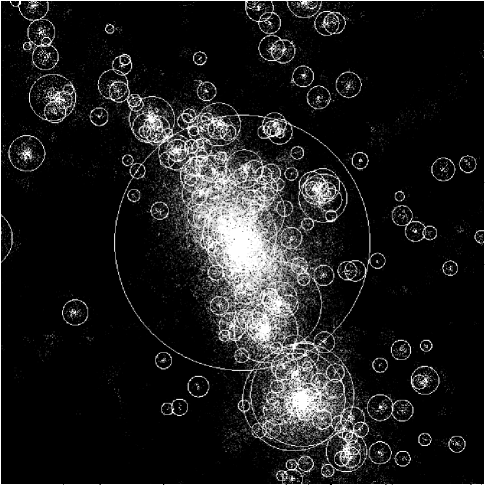
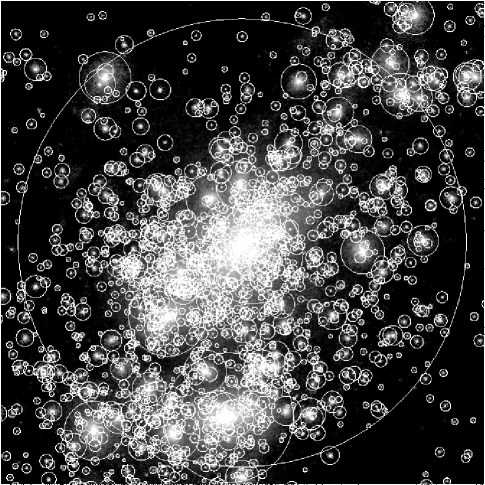
Figure 1: Distribution of dark matter particles (points) and dark matter halos (circles) identified by our halo finding algorithm centered on the most massive halo in the $\Lambda$CDM₈₀ simulation at $z=3$ (left) and $z=0$ (right). The radius of the largest circle indicates the actual virial radius, $R_{180}$, of the most massive halo ($R_{180}=0.67h^{-1}$ comoving Mpc at $z=3$ and $R_{180}=2.1h^{-1}$ Mpc at $z=0$); the radii of all other halos are scaled using the halo’ maximum circular velocities ($r_{\rm h}=0.65V_{\rm max}$ kpc with $V_{\rm max}$ in $\rm km\ s^{-1}$).

3 Halo identification

Identification of DM halos in the very high-density environments of groups and clusters is a challenging problem. The goal of this study is to investigate the halo occupation distribution and clustering of the overall halo population. Therefore, we need to identify both host halos with centers that do not lie within any larger virialized system and subhalos located within the virial radii of larger systems. Below we use the terms satellites, subhalos, and substructure interchangeably.

To identify halos and the subhalos within them we use a variant of the Bound Density Maxima (BDM) halo finding algorithm Klypin et al. (1999, hereafter KGKK). We start by calculating the local overdensity at each particle position using the SPH smoothing kernel of 24 particles. The number of kernel particles roughly corresponds to the lowest halo mass that we hope to identify. We then sort particles according to their overdensity and use all particles with $\delta\geq\delta_{\rm min}=2000$ as potential halo centers. The specific value of $\delta_{\rm min}$ was chosen after experimentation to ensure completeness of the halo catalogs on the one hand while maximizing the efficiency of the halo finder.

Starting with the highest overdensity particle, we surround each potential center by a sphere of radius $r_{\rm find}=50h^{-1}\ \rm kpc$ and exclude all particles within this sphere from further center search. The search radius is defined by the size of smallest systems we aim to identify. We checked that results do not change if this radius is decreased by a factor of two. After all potential centers are identified, we analyze the density distribution and velocities of surrounding particles to test whether the center corresponds to a gravitationally bound clump. Specifically, we construct density, circular velocity, and velocity dispersion profiles around each center and iteratively remove unbound particles using the procedure outlined in Klypin et al. (1999). We then construct final profiles using only bound particles and use them to calculate properties of halos such as maximum circular velocity $V_{\rm max}$, mass $M$, etc.

The virial radius is meaningless for the subhalos within a larger host as their outer layers are tidally stripped. The definition of the outer boundary of a subhalo and its mass are thus somewhat ambiguous. We adopt the truncation radius, $r_{\rm t}$, at which the logarithmic slope of the density profile constructed from the bound particles becomes larger than $-0.5$, as we do not expect the density profile of the CDM halos to be flatter than this slope. Empirically, this definition roughly corresponds to the radius at which the density of the gravitationally bound particles is equal to the background host halo density, albeit with a large scatter. For some halos $r_{\rm t}$ is larger than their virial radius. In this case, we set $r_{\rm t}=R_{\rm vir}$. For each halo we also construct the circular velocity profile $V_{\rm circ}(r)=\sqrt{GM(<r)/r}$ and compute the maximum circular velocity $V_{\rm max}$.

Figure 1 shows the particle distribution in the most massive halos identified at $z=0$ and $z=3$ along with the halos (circles) identified by the halo finder. The particles are color-coded on a grey scale according to the logarithm of their density to enhance visibility of substructure clumps. The radius of circles is proportional to the halo’s $V_{\rm max}$. The figure shows that the algorithm is efficient in identifying substructure down to small masses. Note that the smallest halos plotted in Fig. 1 have masses smaller than our completeness limit of $\approx 50$ particles. This approximate limit corresponds to the mass below which cumulative mass and velocity functions start to flatten significantly. In the following analysis, we will consider only halos with masses $M>50m_{\rm p}$ (corresponding to $1.6\times 10^{9}$ $h^{-1}{\ }{\rm M_{\odot}}$ and $5.4\times 10^{10}$ $h^{-1}{\ }{\rm M_{\odot}}$ in the $\Lambda$CDM₈₀ and $\Lambda$CDM₆₀ boxes respectively).

To classify the halos, we calculate the formal boundary of each object as the radius corresponding to the enclosed overdensity of 180 with respect to the mean density around its center. The halos whose center is located within the boundary of a larger mass halo we call subhalos or satellites. The halos that are not classified as satellites are identified as host halos. Note that the center of a host halo is not considered to be a subhalo. Thus, host halos may or may not contain any subhalos with circular velocity above the threshold of a given sample. The host centers, however, are included in clustering statistics because we assume that each host harbors a central galaxy at its center. Therefore, the total sample of galactic halos contains central and satellite galaxies. The former have positions and maximum circular velocities of their host halos, while the latter have positions and $V_{\rm max}$ of subhalos.

In the observed universe, the analogy is simple. The Milky Way, for example, would be the central galaxy in a host halo of mass $M_{\rm h}\sim 10^{12}h^{-1}\ \rm M_{\odot}$ because its center is not within any larger virialized system. The host halo of the Galaxy contains a number of satellites, which would or would not be included in a galaxy sample depending on how deep the sample is. In a rich cluster, the brightest cluster galaxy that typically resides near the cluster center would be associated with the cluster host halo in our terminology. All other galaxies within the virial radius of the cluster would be considered “satellites” associated with subhalos.

4 Halo Samples

To construct a halo catalog, we have to define selection criteria based on particular halo properties. Halo mass is usually used to define halo catalogs (e.g., a catalog can be constructed by selecting all halos in a given mass range). However, the mass and radius are very poorly defined for the satellite halos due to tidal stripping which alters a halo’s mass and physical extent (see KGKK). Therefore, we will use maximum circular velocity $V_{\rm max}$ as a proxy for the halo mass. This allows us to avoid complications related to the mass and radius determination for satellite halos. Moreover, when a halo gets stripped $V_{\rm max}$ changes less dramatically than the mass, and is therefore a more robust “label” of the halo. For isolated halos, $V_{\rm max}$ and the halo’s virial mass are directly related. For the suhalos $V_{\rm max}$ will experience secular decrease but at a relatively slow rate.

Instead of selecting objects in a given range of $V_{\rm max}$, at each epoch we will select objects of a fixed set of number densities corresponding to (redshift-dependent) thresholds in maximum circular velocity: $n_{i}(>V_{\rm max})$. Note that the number density here includes all the centers of the isolated host halos and the subhalos within the hosts (see eq. 21 in § 7.3).

The threshold selection is somewhat arbitrary, except that the limited box size puts a lower limit on the number densities we can consider. The completeness limit of our catalogs imposes an upper limit on the number densities we can consider. The number densities probed in this simulation span a representative range of galaxy number densities. We chose to focus on a set of number densities corresponding to a representative set of luminosity cuts for SDSS galaxies. Namely, we use the Schechter fit to the SDSS $r$-band luminosity function presented by Blanton et al. (2003) and select the set of galaxy number densities corresponding to the absolute magnitude thresholds $M_{r}=-16$, $-18$, $-19$, $-20$, and $-21$ (the magnitudes quoted are $M-5\log h$). The number densities and corresponding numbers of galactic halos in the analyzed simulations are listed in Table 2. Note that the median redshift of galaxies in the sample of Blanton et al. (2003) is $z=0.1$, while we use simulation outputs at $z=0$. However, using halos at the $z=0.1$ output instead of z=0.0 results in only 2% change in the values of threshold $V_{\rm max}$.

Figure 2: The maximum circular velocity of halos in the $60h^{-1}{\ }{\rm Mpc}$ (dashed line) and $80h^{-1}{\ }{\rm Mpc}$ (solid line) $\Lambda$CDM simulations vs. the $r$-band absolute magnitude of the SDSS galaxies of the same number density. The curves are obtained by matching the cumulative velocity functions $n(>V_{\rm max})$ (at $z=0$) to the SDSS luminosity function $n(<M_{r})$. The dashed lines show the power-law luminosity–circular velocity relation, $L_{r}\propto V_{\rm max}^{a}$, for $a=7$ and $a=3$.

Figure 2 shows the maximum circular velocity of the halos in our simulations with the same number density as the SDSS galaxies with a given $M_{r}$. For comparison the dotted lines show the power law luminosity–circular velocity relation, $L_{r}\propto V_{\rm max}^{a}$, with $a=7$ and $a=3$. Note that the relation does not have a power law form at any circular velocity. For $100<V_{\rm max}<200\rm\ km\ s^{-1}$, the slope is $a\approx 3$, while for $V_{\rm max}<100\rm\ km\ s^{-1}$ the slope is much steeper: $a\approx 7$. Such steepening is of course required to match the shallow faint-end of the galaxy luminosity function with the relatively steep circular velocity function. At $V_{\rm max}\gtrsim 300\rm km\,s^{-1}$, the relation becomes shallow because the number density of halos at these masses is dominated by the central “galaxies” which are assigned maximum circular velocity of their group- or cluster-size host halo. The overall shape of the $M_{r}-V_{\rm max}$ relation thus likely reflects the non-monotonic dependence of the mass-to-light ratio $M_{\rm h}/L$ on the host mass (e.g., Benson et al., 2000b; van den Bosch et al., 2003). The detailed comparisons with the observed Tully-Fisher, however, require more detailed modeling which takes into account effects of baryon cooling on $V_{\rm max}$. At $V_{\rm max}>300\rm\ km\ s^{-1}$, the maximum circular velocity is measured for the host group and cluster-size systems, rather than for the central object, as it is impossible to unambiguously separate the central object from the host group in dissipationless simulations.

Figure 3: Bottom panels: cumulative mass functions of the halo samples (left panel: $\Lambda$CDM₈₀, right panel: $\Lambda$CDM₆₀) used in our analysis at different redshifts. Note that the number density here includes all the centers of the isolated host halos and the subhalos located within the hosts (see eq. 21 in § 7.3). The horizontal dotted lines indicate the number density thresholds adopted in our analysis. The curves were plotted down to the minimum halo mass of 50 particles. Top panels: the fraction of halos with masses larger than $M$ classifed as subhalos: $f_{\rm sub}=(n-n_{\rm host})/n$.

Figure 3 shows the cumulative mass functions for the $\Lambda$CDM₆₀ and $\Lambda$CDM₈₀ simulations at the analyzed epochs. The functions include both centers of the host halos and subhalos and are only plotted down to the mass corresponding to $50$ particles, below which our halo catalogs are incomplete. The horizontal dotted lines show the number density thresholds adopted for the subsequent analysis. Note that at high redshifts the halo catalogs are incomplete at the highest number densities. The figure also shows the fraction of $n(>M)$ that is in objects classified as subhalos. Note that in our samples of galaxy-size halos, about $15-25\%$ of all the halos are in subhalos at any epoch. This is comparable to the observed fraction of $\sim 20\%$ of galaxies located in groups and clusters.

Table 2: Number density thresholds

$n$	SDSS $M_{r}$	$N_{\rm halo}^{80}$	$N_{\rm halo}^{60}$
$h^{3}\ \rm Mpc^{-3}$
$5.86\times 10^{-2}$	-16	30003	12657
$2.79\times 10^{-2}$	-18	14285	6026
$1.52\times 10^{-2}$	-19	7782	3282
$5.89\times 10^{-3}$	-20	3016	1272
$1.11\times 10^{-3}$	-21	568	240

5 The Halo Model

The description of different elements of the halo model can be found in several recent papers (e.g., Seljak, 2000; Ma & Fry, 2000; Peacock & Smith, 2000; Scoccimarro et al., 2001; Sheth et al., 2001a, b; Berlind & Weinberg, 2002; Cooray & Sheth, 2002; Yang et al., 2003). The model has quickly proven to be a very convenient analytic formalism for predicting and interpreting the nonlinear clustering of dark matter and galaxies. The main idea behind the model is that all dark matter is bound up in halos that have well-understood properties. The dark matter distribution is then fully specified by 1) the halo mass function, 2) the linear bias of halos as a function of halo mass, and 3) the radial density profiles of halos as a function of halo mass. These three elements have been relatively well studied using N-body simulations and they can be computed analytically, given a cosmological model. In order to specify the galaxy distribution, two additional ingredients are required: 4) the probability distribution $P(N|M)$ that a halo of virial mass $M$ contains $N$ galaxies and 5) the relative distribution of galaxies and dark matter within halos. These last two elements are called the halo occupation distribution (HOD) and they are only now becoming the focus of much attention both theoretically and observationally (Berlind et al. 2003 and references therein). $P(N|M)$ is the most important piece of the HOD in terms of its effect on galaxy clustering and it is the main focus of this study. We refer to this element when we use the term HOD henceforth.

In the halo model the two-point correlation function of the galaxy distribution is a sum of two terms: the “1-halo” term due to galaxy pairs within a single halo and the “2-halo” term due to pairs in separate distinct halos:

$$\xi_{\rm gg}(r)=\xi^{\rm 1h}_{\rm gg}(r)+\xi^{\rm 2h}_{\rm gg}(r)+1.$$ (1)

At scales larger than the virial diameter of the largest halos, all pairs consist of galaxies in separate halos ($\xi^{\rm 1h}\ll\xi^{\rm 2h}$), while at smaller scales most pairs consist of galaxies within the same halo ($\xi^{\rm 1h}\gg\xi^{\rm 2h}$). The two terms are given by

$$1+\xi^{\rm 1h}_{\rm gg}(r)=\frac{1}{2}\,\bar{n}_{\rm g}^{-2}\int n(M)\langle N(N-1)\rangle_{M}\lambda(r|M)\,dM;$$ (2)

$$\xi^{\rm 2h}_{\rm gg}(r) = \xi^{\rm lin}_{\rm mm}(r)\,\,\bar{n}_{\rm g}^{-2}\int n(M_{1})b_{h}(M_{1})\langle N\rangle_{M_{1}}\,dM_{1}$$ (3)

$$\int n(M_{2})b_{h}(M_{2})\langle N\rangle_{M_{2}}\lambda(r|M_{1},M_{2})\,dM_{2}$$

where $\bar{n}_{\rm g}$ is the mean number density of galaxies in the sample, $n(M)$ is the halo mass function, $b_{h}(M)$ is the large-scale linear bias of halos, $\lambda(r|M)$ is the convolution of the radial profile of galaxies within halos with itself, $\lambda(r|M_{1},M_{2})$ is the convolution of two different radial profiles, and $\xi^{\rm lin}_{\rm mm}(r)$ is the linear dark matter correlation function (also see Sheth et al., 2001b, a; Berlind & Weinberg, 2002). The integration is over the mass limit corresponding to the galaxy sample under consideration.

On large scales, the 2-halo term reduces to $\xi^{\rm 2h}_{\rm gg}(r)=b^{2}\xi^{\rm lin}_{\rm mm}(r)$, where $b$ is the large-scale bias factor of galaxies. Equations 2 and 3 represent the halo model in its most basic form, but variations do exist (see, e.g., Zehavi et al., 2003; Magliocchetti & Porciani, 2003). The halo model is most easily applied in Fourier space because the calculation of the correlation function in real space involves convolutions, which turn into multiplications in Fourier space. For our purposes, however, it suffices to express galaxy clustering in terms of the real-space correlation function.

Equations  2 and 3 show that $\xi^{\rm 2h}$ depends on the average number of galaxies per halo of a given mass,

$$\langle N\rangle_{M}=\sum_{N}NP(N|M),$$ (4)

while $\xi^{\rm 1h}$ depends on the second moment of $P(N|M)$

$$\langle N(N-1)\rangle_{M}=\sum_{N}N(N-1)P(N|M).$$ (5)

Higher order correlations depend on the higher order moments of $P(N|M)$. Both the mean $\langle N\rangle_{M}$ and the shape of $P(N|M)$ are thus key components of the halo model.

For galaxy samples defined by a minimum luminosity threshold, the mean halo occupation $\langle N\rangle_{M}$ is usually assumed to be a power law at high halo masses ($M\gtrsim 10^{13}$ $h^{-1}{\ }{\rm M_{\odot}}$). This is supported both by theoretical models (Berlind et al. 2003 and references therein) and by halo model fits to observational data (e.g., Scoccimarro et al., 2001; Zehavi et al., 2003; Magliocchetti & Porciani, 2003). At low halo masses, $\langle N\rangle_{M}$ is expected to reach a plateau $\langle N\rangle\sim 1$, where each halo contains on average only one galaxy, and then cut off below a minimum mass threshold.

An alternative approach is to assume the existence of two separate galaxy populations: central halo galaxies (zero or one per halo) and satellite galaxies within halos. These populations can then be modeled separately (e.g., Guzik & Seljak, 2002). In particular, in the most simple case the HOD of central galaxies can be modeled as a step function $\langle N_{c}\rangle_{M}=1$ with $\langle N_{c}\rangle_{M}=0$ for $M<M_{\rm min}$, while the HOD of the satellite galaxies can be modeled as a power law, $\langle N_{s}\rangle_{M}\propto M^{\beta}$. The motivation for the separation of central and satellites galaxies comes partly from the analysis of hydrodynamic simulations (Berlind et al., 2003), and partly from studies of central bright elliptical galaxies in groups and clusters, which are often considered as a separate population from the rest of galaxies. As we show below, such a separation greatly simplifies the HOD analysis.

Several simple distributions have been considered for the shape of the HOD. The Poisson distribution is fully specified by its first moment $\langle N\rangle$, as the high-order moments are simply

$$\langle N(N-1)...(N-j)\rangle=\langle N\rangle^{j+1}.$$ (6)

For the nearest integer distribution with $N_{l}\lesssim\langle N\rangle<N_{l}+1$ (where $N_{l}$ is an integer), the second and third moments are

$$\langle N(N-1)\rangle = \langle N\rangle^{2}\left(1+\bar{\xi}_{2}\right)$$

$$\langle N(N-1)(N-2)\rangle = \langle N\rangle^{3}\left(1+3\bar{\xi}_{2}+\bar{\xi}_{3}\right),$$ (7)

where the volume-averaged connected correlations, $\bar{\xi}_{2}(M)$ and $\bar{\xi}_{3}(M)$, are (Berlind et al., 2003)

$$\bar{\xi}_{2} = -\frac{N_{l}(N_{l}+1)}{\langle N\rangle^{2}}+\frac{2N_{l}}{\langle N\rangle}-1,$$

$$\bar{\xi}_{3} = -\frac{2N_{l}(N_{l}^{2}-1)}{\langle N\rangle^{3}}+\frac{6N_{l}^{2}}{\langle N\rangle^{2}}-\frac{6N_{l}}{\langle N\rangle}+2.$$ (8)

For the binomial distribution

$$P(N=n|M)=\frac{{\cal N}_{M}}{n!({\cal N}_{M}-n)!}\,p_{M}^{n}(1-p_{M})^{{\cal N}_{M}-n},$$ (9)

with mean $\langle N\rangle_{M}={\cal N}_{M}p_{M}$, the second moment is $\langle N(N-1)\rangle_{M}={\cal N}_{M}p_{M}({\cal N}_{M}p_{M}-p_{M})$ and the higher-order moments are given by

$$\langle N(N-1)...(N-j)\rangle=\alpha^{2}(2\alpha^{2}-1)...(j\alpha^{2}-j+1)\langle N\rangle^{j+1},$$ (10)

where the parameter $\alpha$ is defined as

$$\alpha^{2}_{M}\equiv\langle N(N-1)\rangle_{M}/\langle N\rangle_{M}^{2}.$$ (11)

The function $\alpha^{2}_{M}$ is a convenient measure of how different $P(N|M)$ is from the Poisson distribution, for which $\alpha^{2}_{M}=1$. For distributions narrower than the Poisson $\alpha^{2}_{M}<1$, while for broader distributions $\alpha^{2}_{M}>1$. Semi-analytic models and hydrodynamic simulations predict a significantly sub-Poisson $P(N|M)$ distribution at low $\langle N\rangle$ (Berlind et al. 2003 and references therein). Moreover, it has been shown that a sub-Poisson $P(N|M)$ distribution is required in order to produce a correlation function of the observed power-law form. (Benson et al., 2000b; Seljak, 2000; Peacock & Smith, 2000; Scoccimarro et al., 2001; Berlind & Weinberg, 2002)

6 Results

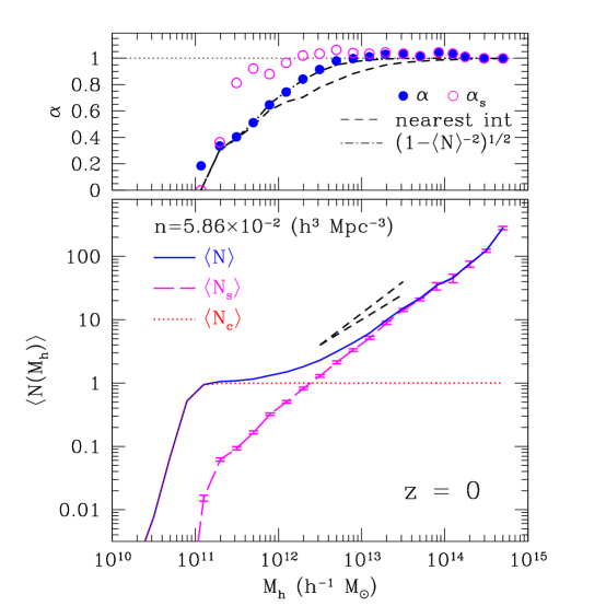
Figure 4: Bottom panel: the first moment of the halo occupation distribution, as a function of host mass for the halo sample with number density $n=5.86\times 10^{-2}h^{3}\rm Mpc^{-3}$ in the $\Lambda$CDM₈₀ simulation at $z=0$. The solid line shows the mean total number of halos including the hosts, while the long-dashed line shows the mean number of satellite halos. The error bars show the uncertainty in the mean. The dotted line shows the step function corresponding to the mean number of “central” halos. Note that by definition, the solid line is the sum of the dotted and long-dashed lines. The two short-dashed lines indicate the dependencies $\propto M_{\rm h}$ and $M_{\rm h}^{0.8}$. Upper panel: the parameter $\alpha\equiv\langle N(N-1)\rangle^{1/2}/\langle N\rangle$ for the full HOD (solid points) and the HOD of satellite halos (open points). The dotted line at $\alpha=1$ shows the case of a Poisson distribution. Note that the HOD becomes sub-Poisson at small host masses. However, the HOD of satellites remains close to Poisson down to masses an order of magnitude smaller than for the full HOD. Indeed, if the satellite HOD is Poisson, $\alpha=(1-1/\langle N\rangle^{2})^{1/2}$ for the full HOD [see eq. (17)]. This expression is shown by the dot-dashed line, which describes the points very well. The full HOD at small $M_{\rm h}$ is also well described by the nearest integer distribution [see eqs. (7) and (8)] shown by the dashed line.

6.1 The Halo Occupation Distribution

We start discussion of our results with the factorial moments of the HOD defined in the previous section. Figure 4 shows the first moment of the HOD for the halo sample with number density of $5.86\times 10^{-2}h^{3}\ \rm Mpc^{-3}$ ($V_{\rm max}>70\ \rm km\,s^{-1}$). Given that the halo samples are constructed by simply selecting all halos with circular velocities larger than a threshold value, the HOD will have a trivial component corresponding to the host halo:

$$N_{\rm c}=\left\{\begin{array}[]{ll}1&\mbox{for $M_{\rm h}\geq M_{\rm min}$}\\ 0&\mbox{for $M_{\rm h}<M_{\rm min}$}\end{array}\right.$$ (12)

where $M_{\rm min}$ is the mass corresponding to the threshold of the maximum circular velocity of the sample. The first moment of this component is simply a step-like function shown in the bottom panel of Figure 4 by the dotted line. Note that halo samples are defined using a threshold $V_{\rm max}$, while the HOD is plotted as a function of halo mass. The transition from zero to unity is therefore smooth because certain scatter exists between $V_{\rm max}$ and halo mass (Bullock et al., 2001b). We find that the scatter is approximately gaussian and its effect on $\langle N_{\rm c}\rangle$ can be described as

$$\langle N_{\rm c}\rangle={\rm erf}(5\,[1-M/M_{\rm min}]).$$ (13)

The second HOD component corresponds to the probability for a halo of mass $M$ to host a given number of subhalos $N_{s}=N-1$: $P_{s}(N_{s}|M)\equiv P(N_{s}+1|M)$. The first moment of this component is shown by the long-dashed line. As we noted above, this separation is equivalent to differentiating between central and satellite galaxies in observations or in semi-analytic models.

The first three moments of $P_{s}(N_{s}|M)$ are related to the moments of the overall HOD as follows

$$\langle N_{s}\rangle = \langle N\rangle-1;$$ (14)

$$\langle N_{s}(N_{s}-1)\rangle = \langle N(N-1)\rangle-2\langle N\rangle+2;$$ (15)

$$\langle N_{s}(N_{s}-1)(N_{s}-2)\rangle = \langle N(N-1)(N-2)\rangle-$$ (16)

$$3\langle N(N-1)\rangle+6\left(\langle N\rangle-1\right).$$

As can be seen from Figure 4, $\langle N_{s}\rangle$ has a simple power law form, while the shape of the full $\langle N\rangle$ (shown by the solid line) is complicated and consists of a step, a shoulder, and the high-mass power-law tail. The parameter $\alpha$ plotted in the upper panel indicates that both $P(N|M)$ and $P_{s}(N_{s}|M)$ are close to Poisson at high masses and become sub-Poisson as the host mass approaches the minimum mass of the sample. However, the satellite HOD can be described by the Poisson distribution down to host masses an order of magnitude smaller than the full HOD. The latter is well described by the nearest integer distribution (see eqs. [7] and [8]) at small $M_{\rm h}$. This result suggests a simple model for the HOD: every host halo contains one halo (itself) and a number of satellite subhalos drawn from a Poisson distribution whose mean is a power-law function of the host halo mass.

Note that the Poisson shape of the subhalo HOD at small masses implies a non-Poisson shape for the overall HOD, as can be seen from equations (14)–(16). For example, for masses where $P_{s}(N_{s}|M)$ is Poisson, we have

$$\alpha^{2}\equiv\frac{\langle N(N-1)\rangle}{\langle N\rangle^{2}}=1-\frac{1}{\langle N\rangle^{2}},$$ (17)

which shows that the shape is Poisson ($\alpha^{2}=1$) at high masses but drops to zero at low masses. The HOD thus starts to deviate from Poisson significantly at $\langle N\rangle\lesssim 4$: e.g, $\alpha^{2}=0.81$ for $\langle N\rangle=2.3$, while $\alpha^{2}=0$ for $\langle N\rangle=1$. As can be seen in the upper panel of Figure 4, equation (17) describes $\alpha$ measured in the simulation very well.

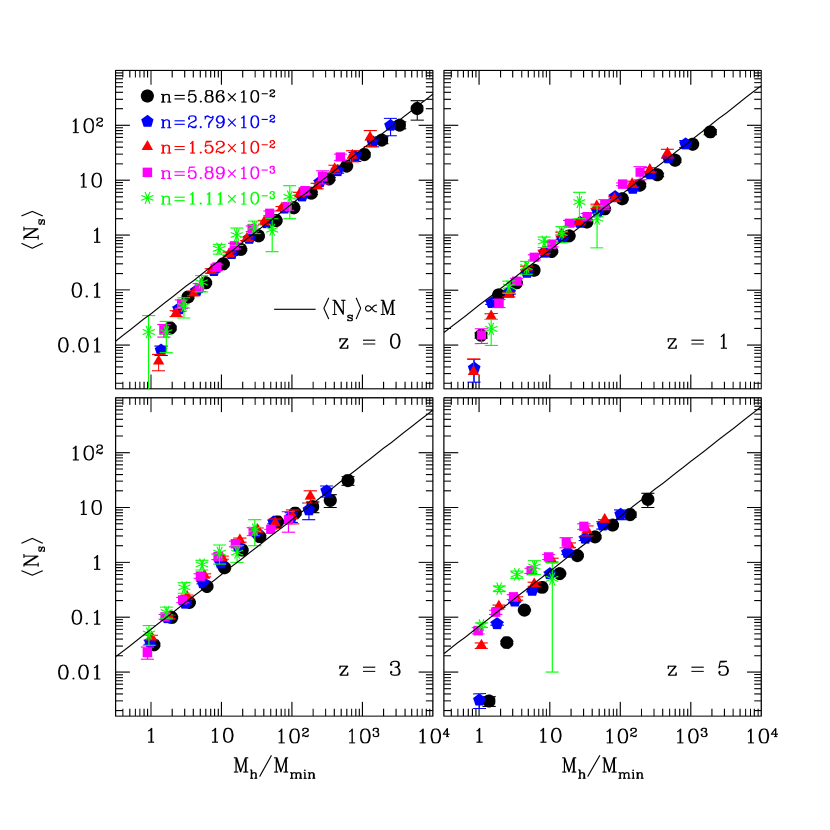
Figure 5: The mean number of subhalos $\langle N_{s}\rangle$ as a function of host mass for the halo samples of different number densities (symbols of different type) at different redshifts. The error bars show the uncertainty in the mean. The mean is plotted as a function of host mass in units of the minimum mass of the sample (see Fig. 3; note that, by definition, $\langle N_{s}\rangle=0$ at $M_{\rm h}/M_{\mathrm{min}}=1$ and non-zero points shown at or below $M_{\rm h}/M_{\mathrm{min}}=1$ are caused by binning). The mass $M_{\rm h}$ in the $x$-axis is the mass within the radius corresponding to overdensity 180 with respect to the mean density of the universe. The number densities in units of $h^{3}\rm Mpc^{-3}$ are indicated in the legend. The solid line in each panel shows the linear relation $\langle N_{s}\rangle\propto M_{h}$. The figure shows that the mean number of subhalos at different number densities is remarkably similar and shows only a mild evolution. The mass dependence is approximately linear $\langle N_{s}\rangle\propto M_{\rm h}$ for masses $M_{\rm h}/M_{\rm min}\gtrsim 5$ (or $\langle N_{s}\rangle\gtrsim 0.2).$

Figure 5 shows the mean of the subhalo HOD, $\langle N_{s}\rangle$, for different epochs and samples of different number densities. The mean is plotted as a function of mass in units of the minimum mass of the sample, $\mu\equiv M_{\rm h}/M_{\rm min}$. The figure shows that the mean number of subhalos as a function of $\mu$ at different number densities is remarkably similar and exhibits only a weak evolution with time. The mass dependence is approximately linear $\langle N_{s}\rangle_{\mu}\propto\mu$ for masses $\mu\gtrsim 5$ (or $\langle N_{s}\rangle\gtrsim 0.2).$ The formal linear fits to the $\langle N_{s}\rangle_{M}$ of individual samples result in best fit slopes close to unity for $M_{\rm h}/M_{\rm min}\gtrsim 5$ with rather small deviations from the linear behavior. The best fit slopes for the samples of different number densities at $z=0$ are $0.99\pm 0.01$, $0.92\pm 0.03$, $0.96\pm 0.08$, $1.04\pm 0.08$, and $0.61\pm 0.21$ in the order of the decreasing number density. As a function of redshift, the best fit slopes for the sample of $n=5.86\times 10^{-2}h^{3}\rm\ Mpc^{-3}$ are $1.03\pm 0.01$, $1.05\pm 0.02$, $1.18\pm 0.05$, $1.28\pm 0.04$, for $z=0,1,3,5$, respectively.

Although $\langle N_{s}\rangle$ is close to the power law for most of the most of the mass range, the deviations from power law are evident at $M\sim M_{\rm min}$, especially at low redshifts. A more accurate formula describing the first moment is

$$\langle N_{s}\rangle=(M/M_{1}-C)^{\beta},$$ (18)

where $M_{1}$ is normalization, defined as $\langle N_{s}(M_{1})\rangle=1$, and $C$ is a constant for a given redshift. Parameters $M_{1}$ and $C$ exhibit mild evolution with redshift. For $z=0$, $C\approx 0.045$ or $M_{1}/M_{\rm min}\approx 22$.

The slope of the high-mass tail of $\langle N\rangle_{M}$, $\beta$, is one of the key factors determining galaxy clustering statistics. In our results the asymptotic slope of $\langle N_{s}\rangle$ in the total mean $\langle N\rangle$ is reached only at relatively high masses. A linear fit at intermediate masses is likely to result in a shallower slope. Thus, for example, a power-law fit $\langle N\rangle\propto M^{\beta}$ to the full HOD shown in Figure 4 for $\langle N\rangle>4$ gives $\beta=0.87\pm 0.01$, while the fit to $\langle N_{s}\rangle$ for the same range of masses gives $\beta_{s}=1.03\pm 0.01$. This may explain the smaller than unity slopes of the mean occupation number obtained in several theoretical and observational analyses (e.g., Berlind et al. 2003; Zehavi et al. 2003). These estimates may therefore be underestimates of the true asymptotic high-mass slope.

Figure 6 shows a comparison of the $\langle N_{s}\rangle_{M}$ for the $n=2.79\times 10^{-2}h^{3}\rm\ Mpc^{-3}$ halo sample in the $\Lambda$CDM₈₀ and $\Lambda$CDM₆₀ simulations at $z=0$ and $z=3$. The subhalo HODs in the two runs agree well over the most of the mass range at both epochs. The shape of $P_{s}(N_{s}|\mu)$, therefore, is not sensitive to the normalization of the power spectrum. The systematically lower values of $\langle N_{s}\rangle$ at low $M_{\rm h}/M_{\rm min}$ in the $\Lambda$CDM₆₀ simulation are expected. Halos in this higher-$\sigma_{8}$ cosmology form earlier and disruption processes have more time to operate and lower the number of satellites with masses comparable to that of the host. This difference can also be partly due to the limited mass resolution of the simulations.

Figure 6: The mean number of subhalos $\langle N_{s}\rangle$ as a function of host mass for the halo samples with number density $n=2.79\times 10^{-2}h^{3}\rm Mpc^{-3}$ in the $\Lambda$CDM₆₀ (open circles) and $\Lambda$CDM₈₀ (filled circles) at $z=0$ (top panel) and $z=3$ (bottom panel). The error bars show the uncertainty in the mean and are smaller than the symbols. The mean is plotted as a function of host mass in units of the minimum mass of the sample (see Fig. 3). The solid line in each panel shows the linear relation $\langle N_{s}\rangle\propto M_{h}$. The figure shows that the HOD for a given $M_{\rm h}/M_{\rm min}$ is not sensitive to normalization of the power spectrum.

In Figure 7 we plot the square root of the second and the cube root of the third moments of the subhalo HOD for the samples and epochs shown in Figure 5. For comparison the solid lines show the linear function $\langle N_{s}\rangle\propto\mu$ of the same amplitude as in the corresponding panel of Figure 5. Figure 7 shows that $\langle N_{s}\rangle\approx\langle N_{s}(N_{s}-1)\rangle^{1/2}\approx\langle N_{s}(N_{s}-1)(N_{s}-2)\rangle^{1/3}$ for $\mu\gtrsim 5$, as expected for the Poisson distribution (eq. [6]). Therefore, $P_{s}(N_{s}|\mu)$ can be described by the Poisson distribution at these masses. As in the case of the mean, the higher moments of the subhalo HOD have similar shape and amplitude as a function of $\mu$ for different number densities and redshifts.

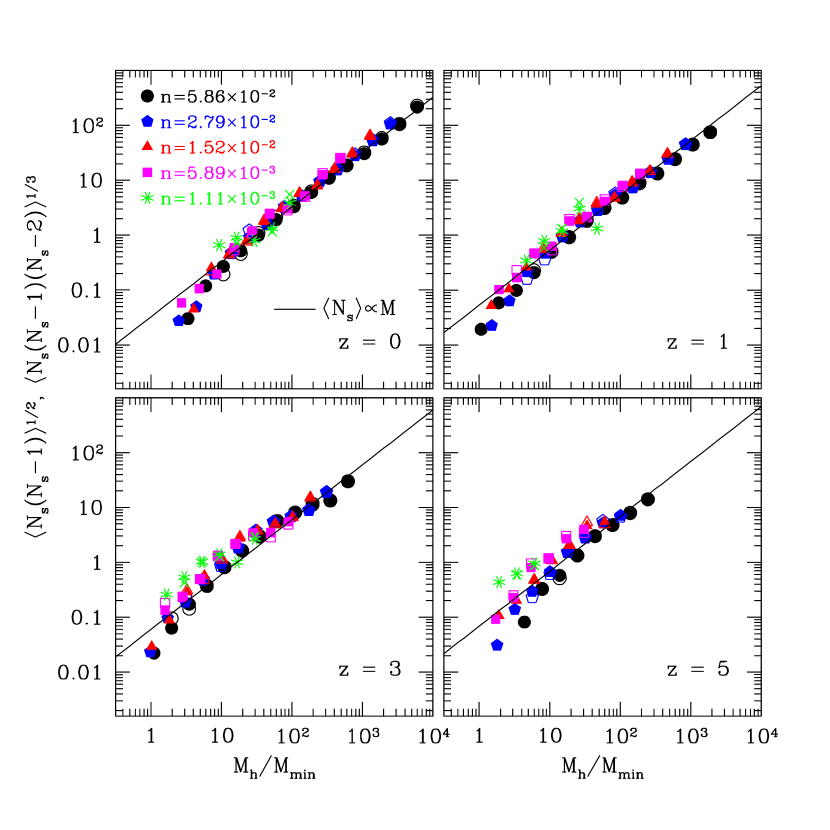
Figure 7: The square root of the second moment, $\langle N_{s}(N_{s}-1)\rangle^{1/2}$ (filled symbols), and the cube root of the third moment$\langle N_{s}(N_{s}-1)(N_{s}-2)\rangle^{1/3}$ (open symbols, except for the lowest number density which is shown by crosses) for the halo samples of different number densities (symbols of different type) at different redshifts. The moments are plotted as a function of host mass in units of the minimum mass of the sample. The number densities in units of $h^{3}\rm Mpc^{-3}$ are indicated in the legend. The solid line in each panel shows the linear relation $\langle N_{s}\rangle\propto M_{h}$ of the same amplitude as the solid line in the corresponding panel of Figure 5. The figure shows that the HODs at different number densities and epochs are remarkably similar and are close to the Poisson distribution at $M_{\rm h}/M_{\rm min}\gtrsim 5$ (or $\langle N_{s}\rangle\gtrsim 0.2-0.3$).

6.2 The halo 2-point correlation function

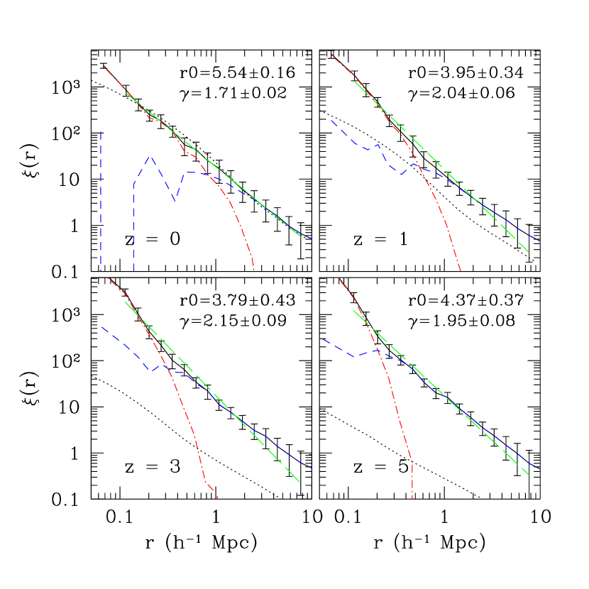
Figure 8: Evolution of the two-point correlation function in the $80h^{-1}\ \rm Mpc$ simulation. The solid lines with error bars show the clustering of halos of fixed number density $n=5.89\times 10^{-3}h^{3}\ \rm Mpc^{-3}$ at each epoch. The error-bars indicate the “jack-knife” one sigma errors, computed using the eight octants of the simulation cube, and are larger than the Poisson error at all scales. The dot-dashed and dashed lines show the corresponding one- and two-halo term contributions. The long-dashed lines show the power-law fit to the correlation functions in the range of $r=\left[0.1-8h^{-1}\ \rm Mpc\right]$. Although the correlation functions can be well fit by a power law at $r\gtrsim 0.3h^{-1}\ \rm Mpc$ in each epoch, at $z>0$ the correlation function steepens significantly at smaller scales due to the one-halo term. For comparison, the dotted lines show the correlation function of the dark matter.

In this section we present the two-point correlation functions (CFs) for the halo samples used in the analysis of the HODs. Figure 8 shows the CFs for the sample of $n=5.89\times 10^{-3}h^{3}\ \rm Mpc^{-3}$ at $z=5$, $3$, $2$, and $0$, as well as their one- and two-halo components. The error bars shown for the CFs are the errors in the mean, estimated from jack-knife resampling using the eight octants of the simulation cube (see Weinberg et al., 2003), and they are dominated by the “cosmic variance” of the finite number of coherent structures in the simulation volume. Several interesting features are immediately apparent. First, at scales $\gtrsim 0.3h^{-1}\ \rm Mpc$ the CFs at all epochs can be well described by a power law, $\xi(r)=(r/r_{0})^{-\gamma}$, with only mildly evolving amplitude and slope. The amplitude of the dark matter correlation function, on the other hand, increases with redshift revealing strongly time-dependent bias. At the present-day epoch, there is a slight antibias at $r\lesssim 1h^{-1}\ \rm Mpc$. Interestingly, the magnitude of the anti-bias is considerably smaller than in the higher-normalization ($\sigma_{8}=1$) simulation (see Fig. 7 in Colín et al. (1999) as well as Fig. 9 in this paper). This is consistent with the picture where the anti-bias is caused by the halo disruption processes in high-density regions (Kravtsov & Klypin, 1999), as groups and clusters in the low-normalization model form later and the disruption processes have less time to operate. The exclusion effect in the two-halo component is significant at $z=0$, but diminishes at earlier epochs. This is due mainly to the systematic decrease in the minimum mass of the sample for the same number density at higher $z$. The smaller minimum mass means smaller halo sizes. The smaller size is also due to the definition of the virial radius with respect to the mean density. Even for the same mass higher mean density of the Universe at higher redshifts results in a smaller virial radius. Smaller sizes of halos in the sample result in smaller minimum pair separation for isolated objects. Thus, 2-halo term extends to smaller $r$.

At $z=0$ the halo CF can be well approximated by a power law at all probed scales ($0.1-10h^{-1}\ \rm Mpc$). The approximate power-law shape is due to the relatively smooth transition between the two- and one-halo components of the CF. At higher redshifts, however, the transition is more pronounced and occurs at progressively smaller scales. This results in a significant steepening of the CF at $\sim 0.3-1h^{-1}\ \rm Mpc$. The halo model analysis shows that contribution of pairs in massive galaxy clusters is critical for a smooth transition between 1- and 2-halo contributions (Berlind & Weinberg, 2002). At earlier epochs, clusters are rare or non-existent which explains a more pronounced transition.

Indeed, power-law fits using the range of scales $0.1-8h^{-1}\ \rm Mpc$ give systematically smaller values of the scale radius $r_{0}$ and steeper slope $\gamma$ than the fits over range $\sim 0.3-8h^{-1}\ \rm Mpc$, as can be seen in Figure 12. All of the fits for the $\Lambda$CDM₈₀ simulations are performed at $r\leq 8h^{-1}\ \rm Mpc$, as the CF shape becomes affected at scales larger $>0.1L_{\rm box}$ (Colín et al., 1997, 1999). We also checked this by comparing matter correlation functions in the simulation to the model of Smith et al. (2003). We find that simulation results agree well with the model at scales $<0.1L_{\rm box}$ at $z=0$ and at $<0.2-0.3L_{\rm box}$ at higher redshifts.

The power-law shape of the correlation function is rather remarkable, as it appears to result from a sum of non-power law components. We checked the components of the correlation function due to pairs of different types: central-satellite, satellite-satellite, and central-central pairs. The component CFs have a variety of shapes all deviating strongly from power law. Yet, the sum is close to the power law. This indicates that the power-law shape of the galaxy correlation function may well be a coincidence, as noted by Benson et al. (2000b) and Berlind & Weinberg (2002).

Figure 9: The correlation function and bias for the $n=1.52\times 10^{-2}h^{3}\ \rm Mpc^{-3}$ sample in the $\Lambda$CDM₆₀ (dashed) and $\Lambda$CDM₈₀ (solid) simulations. Top panel: The bias $b(r)\equiv\sqrt{\xi_{\rm hh}(r)/\xi_{\rm mm}(r)}$. Bottom panel: The halo-halo correlation function in the two simulations compared to the correlation function of the APM galaxies (Baugh, 1996). The error-bars indicate the “jack-knife” one sigma errors, computed using the eight octants of the simulation cube, and are larger than the Poisson error at all scales.

Figure 10: The projected correlation function of the bright ($M_{r}<-21$) galaxies in the SDSS volume-limited sample (Zehavi et al., 2003) compared to the $z=0$ projected correlation function of halo samples of three different number densities indicated in the legend. Note that $M_{r}<-21$ galaxies have number density of $1.1\times 10^{-3}h^{3}\ \rm Mpc^{-3}$. The figure shows that the correlation functions of galaxies and halos of the same number density are in good agreement (see text for discussion).

Comparing the correlation functions in the $\Lambda$CDM₆₀ and $\Lambda$CDM₈₀ simulations (Figure 9), we find that the correlation functions of objects with the same number density are similar. This is not surprising in light of the approximate universality of the HOD demonstrated in the previous section (see Figs. 5 and 6). Figure 9 also shows that the amplitude and shape of the CF at $z=0$ is in good agreement with that of the galaxies in the APM survey. As noted by Kravtsov & Klypin (1999) and Colín et al. (1999), the close agreement of halo and galaxy correlation functions indicates that the overall clustering of the galaxy population is determined by the distribution of their dark matter halos.

Figure 10 shows a comparison of the projected correlation functions:

$$w_{p}(r_{p})=2\int\limits^{r_{\rm max}}_{0}\xi([r_{p}^{2}+y^{2}]^{1/2})dy,$$ (19)

in the volume-limited sample of bright, $M_{r}<-21$, galaxies (Zehavi et al., 2003) and halo samples of three representative number densities in the $\Lambda$CDM₈₀ simulation. The upper integration limit was set to $r_{\rm max}=40h^{-1}\ \rm Mpc$, to mimick the procedure used to estimated the observed CF. In taking the projection integral, we extrapolate the simulated CF from $8h^{-1}$ Mpc (the largest reliable scale of the simulation) to large scales using the correlation function of dark matter predicted by the Smith et al. (2003) model rescaled to match the amplitude of the halo correlation function at $8h^{-1}$ Mpc. Note that the SDSS galaxies have a number density of $1.1\times 10^{-3}h^{3}\ \rm Mpc^{-3}$ and their CF should therefore be compared to the solid line. The figure shows that the correlation functions of galaxies and halos in our simulations agree remarkably well. In particular, the steepening of the observed correlation function at $r\lesssim 1h^{-1}\ \rm Mpc$ is reproduced. The difference at large scales is not significant given the large sample variance errors in the halo correlation function that result from the small size of the simulation cube (see Figures 8 and 9).

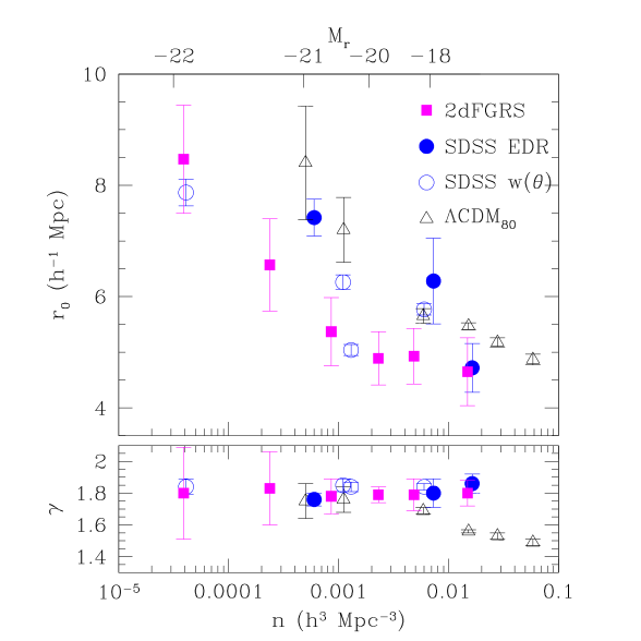
Figure 11: Top panel: the best-fit correlation scale $r_{0}$ as a function of number density at the present day epoch. The results for the dark matter halos (open triangles) are compared to the recent measurements of galaxy clustering in the SDSS (solid circles are from the analysis of the Early Data Release by Zehavi et al. (2002), while open circles are derived from the analysis of the angular correlations by Budavari et al. (2003)) and 2dF surveys (solid squares; Norberg et al., 2002). The upper axis shows the $r$-band absolute magnitude for the SDSS galaxies corresponding to each number density. The power-law fits were done over the range of scales from $0.3$ to $8h^{-1}\ \rm Mpc$. Bottom panel: the best-fit slope of the correlation function as a function of number density.

Large galaxy redshift surveys have been used to detect a luminosity dependence of galaxy clustering (e.g., Guzzo et al., 1997; Willmer et al., 1998; Norberg et al., 2001; Zehavi et al., 2002). There are indications that a similar dependence exists at early epochs (e.g., Giavalisco & Dickinson, 2001). As the luminosity of galaxies is expected to be tightly correlated with the halo maximum circular velocity or mass, the luminosity-dependence of clustering should be reflected in the mass-dependence of halo clustering. Figures 11 and 12 show the best-fit correlation length $r_{0}$ and slope $\gamma$ as a function of sample number density, with lower number densities corresponding to samples of halos with larger mass (i.e., larger values of threshold $V_{\rm max}$). Figure 11 shows the $z=0$ results compared to the 2dF (Norberg et al., 2001) and SDSS galaxy surveys (Zehavi et al., 2002; Budavari et al., 2003). The figure shows that the dependence of halo clustering on sample number density in our simulation is in general agreement with the SDSS Early Data Release results (Zehavi et al., 2002).

The simulation points are systematically higher than the 2dF and Budavari et al. (2003) results. Note, however, that the upturn in the clustering amplitude occurs at approximately the same number density, $n\approx 2-4\times 10^{-3}h^{3}\ \rm Mpc^{-3}$, in the simulation and 2dF survey. The difference in amplitude can likely be attributed to the fact that 2dF galaxies are selected using a blue-band magnitude, since several recent studies have shown that redder galaxies are clustered more strongly (e.g., Norberg et al., 2001; Zehavi et al., 2002). In addition, the halo samples include all objects above a threshold circular velocity, while most of the observational points in Figure 11 are defined for galaxies in (broad) luminosity ranges.

Interestingly, all of the observational estimates indicate that the slope of the CF does not depend strongly on the luminosity. The slope of the halo CF is in agreement with observations for $n<0.01h^{3}\ \rm Mpc^{-3}$ but becomes shallower for smaller mass objects. At $n\approx 0.02h^{3}\ \rm Mpc^{-3}$ the slope for the halo sample is significantly shallower than that for the galaxies in the 2dF and SDSS surveys. This indicates that luminosity dependence of the CF slope may provide additional useful constraints on galaxy formation. The exercise demonstrates that both slope and correlation length should be compared when model predictions are confronted with observations.

Mass dependence of the clustering amplitude is also found at earlier epochs (Fig. 12). The clustering of halos at $z=3$ is in reasonable agreement with clustering of Lyman break galaxies (LBGs, Adelberger, 2000; Adelberger et al., 2003). The detailed comparison is complicated due to the often contradictory results from analyses that use different LBG samples and methods (for a summary of recent results see Bullock, Wechsler, & Somerville, 2002, and § 7 below). An important point is that, as we noted above, at higher redshifts the steepening of the CF at small scales biases results if a single power-law is fit down to small scales. This bias can be clearly seen in Figure 12, which shows the best-fit scale radius and slope for the power-law fits down to both $0.1h^{-1}\ \rm Mpc$ and $0.3h^{-1}\ \rm Mpc$. At both $z=1$ and $z=3$, fits to smaller scales result in smaller $r_{0}$ and larger absolute values of the slope $\gamma$.

7 Discussion

7.1 Implications for galaxy clustering

The results presented in the previous sections show that the main properties of the observed clustering of galaxies are imprinted in the distribution of their surrounding halos. The term halo here includes both the isolated halos and the distinct gravitationally-bound subhalos within the virialized regions of larger systems.

The shape and evolution of the two-point correlation function and the mass-dependence of clustering amplitude for these subhalos are in good agreement with constraints, for galaxies of similar number densities, from recent observational surveys at a range of redshifts. In addition, the halo occupation distribution derived in this study for the subhalos is similar to the HOD obtained for the galaxies in semi-analytic analyses and for cold gas clumps in gasdynamics simulations (Berlind et al., 2003). All of these are consistent with present observational constraints on the galaxy HOD (e.g., Zehavi et al., 2003), for galaxies of similar number densities; however, observational measurements of the HOD are not yet robust enough to make a meaningful comparison. The test of our predictions against real data must thus await future measurements.

This result has several implications. First and foremost, it means that the formation of halos and their subsequent merging and dynamical evolution are the main processes shaping galaxy clustering. This appears to be true for the clustering of halo samples with maximum circular velocities larger than a given threshold value, which were the focus of the present and other recent studies (Kravtsov & Klypin, 1999; Colín et al., 1999; Neyrinck et al., 2003). This type of halo sample should correspond to volume-limited samples of galaxies with luminosities above a certain threshold value because the maximum circular velocity of a halo is expected to be tightly correlated with the luminosity of the galaxy it hosts. The caveat, of course, is that we can expect a considerable band-dependent scatter between galaxy luminosity and $V_{\rm max}$, which needs to be accounted for in the model. The inclusion of scatter is relatively straightforward and future analysis will show just how large the effect of scatter is.

Useful constraints on galaxy evolution and better understanding of galaxy clustering can be obtained by more sophisticated analyses. For example, it would be interesting to compare the HOD of galaxies of different colors (e.g., Zehavi et al., 2002) with that of halos with different merger histories or environments, which would likely provide insight into the formation of galaxies of different types.

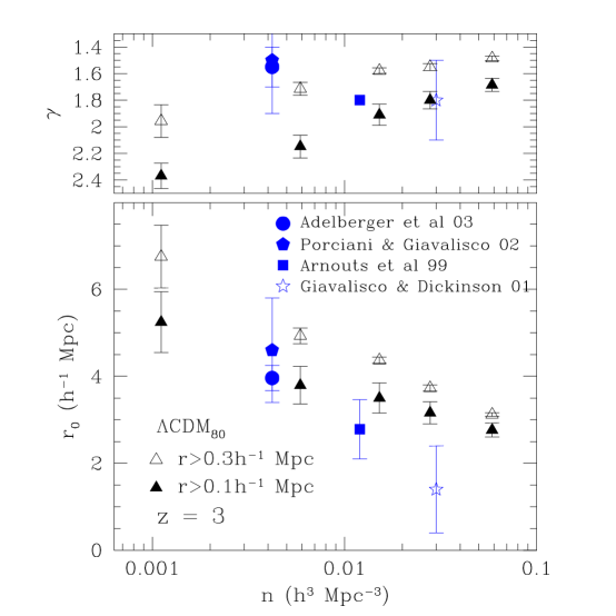
Figure 12: The same as in Fig. 11 but for $z=1$ and $z=3$. At high redshifts the correlation function significantly steepens at small separations due to the one-halo correlations (see Fig. 8). This makes the results of the power-law fit sensitive to the minimum separation $r_{\rm min}$ used in the fit. The figure shows results for two values $r_{\rm min}$: $100h^{-1}\ \rm kpc$ (solid triangles) and $300h^{-1}\ \rm kpc$ (open triangles). At $z=3$ the results are compared to the recent observational measurements of Lyman Break Galaxy clustering at $z\sim 3$.

One of the most interesting features of galaxy clustering is the approximately power-law shape of the two-point correlation function. Although departures from a power law have been found (Zehavi et al., 2003), they are quite small. This has been and still is a major puzzle in galaxy formation studies, especially in light of the strong deviations from the power-law behavior seen in the dark matter correlation function (Klypin et al., 1996; Jenkins et al., 1998). In the framework of the recently developed halo model, there also does not seem to be a generic way to produce a purely power-law CF (Berlind & Weinberg, 2002). The power-law shape thus appears to be somewhat of a coincidence.

Without a doubt, the fact that the (approximately) power-law CF observed for galaxies is reproduced with subhalo populations identified in simulations with the correct slope and amplitude at $z=0$ down to scales $<100h^{-1}\ \rm kpc$ can be viewed as a significant success. The power-law nature of the correlation fucntion is due to a relatively smooth transition between its one- and two-halo terms. At higher redshifts this transition is more pronounced and the CF steepens at small scales. The transition scale decreases with increasing redshift, reflecting the decrease in the average halo size with time. The key to the puzzle of the power-law shape of the CF thus appears to be in understanding the transition between the one- and two-halo terms.

Interestingly, if similar large departures from a power law exist for real high-redshift galaxies, this may bias observational power-law fits and explain some of the discrepancies between observational analyses. For example, as can be seen in Figure 12, single power-law fits to smaller radii result in systematically smaller values of $r_{0}$ and steeper slopes $\gamma$. If the slope is kept fixed, as is often done in analyses of high-$z$ galaxy clustering, the derived correlation length may be artificially large. Using the halo model formalism, Zheng (2003) recently showed that the large correlation length inferred for red galaxies at $z\approx 3$ by Daddi et al. (2003) can be explained by the steepening of the CF at small scales, as observed for subhalos in our simulation. Daddi et al. (2003) studied clustering of red galaxies in the Hubble Deep Field South. The number density and range of radii probed in their study are $n\approx 7\times 10^{-3}h^{3}\ \rm Mpc^{-3}$ and $\sim 0.04-1h^{-1}$, with the statistically significant correlations detected only for $r\lesssim 400h^{-1}\ \rm kpc$. All scales here and below are computed assuming the flat $\Lambda$CDM cosmology adopted in this paper. Given a limited number of radial bins, Daddi et al. (2003) used a power-law fit to the angular correlation function with a fixed slope of $-0.8$ and obtained the best fit correlation length of $r_{0}\approx 8h^{-1}\ \rm Mpc$.

As a comparison, for the halo sample with the number density of $6\times 10^{-3}h^{3}\ \rm Mpc^{-3}$ in our simulation, a weighted least squares fit over the interval $40-400h^{-1}\ \rm kpc$ with the slope fixed to $-1.8$ gives $r_{0}=7.85\pm 0.77h^{-1}\ \rm Mpc$, remarkably close to the value derived by Daddi et al. (2003). This, however, is simply a reflection of steepening of the CF at small scales. If both the slope and the correlation length are allowed to vary, best fit values for the same range of scales are $r_{0}=2.04\pm 0.76h^{-1}\ \rm Mpc$ and $\gamma=2.69\pm 0.18$. At the same time, the correlation function is unity at $r_{0}\approx 5h^{-1}\ \rm Mpc$ and the power-law fit over the interval $0.3-8h^{-1}\ \rm Mpc$ gives $r_{0}=4.93\pm 0.49h^{-1}\ \rm Mpc$ and $\gamma=1.72\pm 0.13$ (see Fig. 12), in very good agreement with the halo model calculations of Zheng (2003).

Similar biases may explain some of the discrepant results on the clustering of Lyman break galaxies (LBGs), virtually all of which have assumed a power-law correlation function, and many of which have fixed the power-law slope during fits. Many studies presented seemingly contradictory measurements of correlation lengths ranging from 1 to $5h^{-1}$ Mpc (Giavalisco & Dickinson, 2001; Bullock et al., 2002; Adelberger et al., 2003; Porciani & Giavalisco, 2002; Arnouts et al., 1999). The variety of values and discrepancies of the correlation length and slope could be explained by departures of the high-$z$ CF from the single power law. Thus, for example, the power-law fit over the smallest angular scales in the HDF sample by Giavalisco & Dickinson (2001) gives the smallest value of $r_{0}$ and the steepest slope $\gamma$. The analysis of Arnouts et al. (1999) fits the CF over a larger range of scales with the slope fixed at a relatively low value and results in a larger value of $r_{0}$. This would be expected if the CF steepens at small scales, as observed in our simulations. All of the studies perform the Limber deprojection assuming a power-law CF, which may further bias results. The implication is that if the deviations from the power law for the galaxy CF are as strong as indicated by our results, the assumption of the single power law is dangerous and is likely to bias results. The magnitude of the bias depends on the range of scales probed and the analysis method.

On the positive side, the sharper transition from one- to two-halo components of the CF at early epochs means that departures from the power law may be easier to detect in high-redshift surveys than they are at $z=0$. Such features can be useful in understanding the environments and nature of galaxies because the one-halo term contains information about $P(N|M)$ and the radial distribution of galaxies in halos. For example, we can expect the distribution of red galaxies to be biased toward the high-density regions of groups and clusters. Their correlation function is therefore expected to have a more pronounced one-halo term. Although the sizes of samples are still relatively small at present, it is interesting that the projected CF of the largest LBG galaxy samples to date presented by Adelberger et al. (2003) (their Fig. 23; see also Hamana et al., 2003) indicates a departure from the power law similar to that in $z=3$ panel of Fig. 8.

7.2 The shape of the halo occupation distribution

The main result of our study is the approximate universality of the halo occupation distribution, $P_{s}(N_{s}|\mu)$ where $\mu\equiv M/M_{\rm min}$, for the subhalos in our samples. We show that the overall HOD can be split into the probability for a halo of mass $M$ to host a central galaxy and its probability to host a given number $N_{s}$ of satellite galaxies, which significantly simplifies the halo model. The former can be approximated by a step function, while the latter is well approximated by the Poisson distribution fully specified by its first moment $\langle N_{s}\rangle$ for $\mu\gtrsim 5$. The first moment of the distribution is well represented by a simple power law $\langle N\rangle\propto\mu^{\beta}$ for $\mu\gtrsim 5$ with $\beta$ close to unity for a wide range of number densities and redshifts. We also find that the form of the satellite HOD is not sensitive to the normalization of the power spectrum. Note that although the amplitude of $\langle N\rangle(\mu)$ changes little for different number densities, redshifts, and spectrum normalizations, some weak dependencies do exist. Thus, for example, the first moment for the lower number density (i.e., higher mass) samples have a systematically higher amplitude. Moreover, there is a factor of three increase in the normalization from $z=0$ to $z=5$. The HOD moment in the lower-normalization simulation has a slightly higher amplitude than in the higher normalization run (Fig. 6).

It is worth noting that results presented here for the dark matter halos are in good agreement with the results of semi-analytic and gasdynamics simulations obtained by Berlind et al. (2003). In particular, we checked that our results on the HOD of the satellite galaxies are in very good agreement with the results of these simulations.

The approximately linear dependence of the first moment on the host mass, $\langle N_{s}\rangle\propto M$, is related to the shape of the subhalo mass and velocity functions: $N_{s}(>V_{\rm sub})=A({V_{\rm sub}/V_{\rm h})^{-\eta}}$, where $N_{s}$ is the number of subhalos within the virial radius of the host and $V_{\rm sub}$ and $V_{\rm h}$ are the maximum circular velocity of subhalos and the host, respectively. High-resolution simulations give $\eta\approx 3$ (Klypin et al., 1999; Moore et al., 1999) and normalization approximately independent of mass $A\approx{\rm const}$ (Moore et al., 1999; Colín et al., 2003). Therefore, the number of subhalos with $V_{\rm sub}$ above a certain threshold $V_{\rm th}$ scales as $N_{s}(>V_{\rm th}|M_{h})=AV_{\rm th}^{-\eta}V_{\rm h}^{\eta}$. The circular velocity of isolated host halos is tightly correlated with their mass $M_{\rm h}=CV_{\rm h}^{a}$ with $a\approx 3-3.3$ (e.g., Avila-Reese et al., 1999; Bullock et al., 2001b). We thus have $N(>V_{\rm th}|M_{h})\propto M_{\rm h}^{\beta}$ with $\beta={\eta/a}\sim 1$.

The simple combination of a step function representing the central galaxies and a Poisson distribution for the satellite galaxies can be compared to the sum of the HODs for the two, which is in general significantly more complicated, consisting of a step, a shoulder, and a power-law high mass tail, as observed in our simulations and in simulations studied by Berlind et al. (2003). This shape is sometimes approximated simply by a power law (e.g., Bullock et al., 2002) or by the combination of a step function and a power law for masses larger than some $M_{p}$ (e.g., Zehavi et al., 2003). However, these are only crude approximations, as the first moment of the HOD in simulations is almost never flat, especially at high redshifts. Modeling of the HOD as a combination of host and satellite HODs provides a considerably more accurate prescription without increasing the number of parameters. It is also more physically motivated because it is reasonable to expect that the processes that control the formation of the central galaxy are different from those that control the abundance of satellite galaxies.

Most importantly, the simple form of the satellite HOD hints at some simple physical processes that control the satellite population. Understanding these processes is well within the capabilities of current numerical simulations or semi-analytic models for satellite accretion and orbital evolution (e.g., Bullock et al., 2000; Zentner & Bullock, 2003). Further theoretical studies of the satellite HOD should thus provide key clues to the understanding of small-scale galaxy bias and the power-law shape of the correlation function.

7.3 Halo occupation distribution model

Our results suggest a simple yet accurate model for the halo occupation distribution for samples selected with a given mass or luminosity threshold, which could be used in theoretical modeling and model fits to the observational data. The probability for a halo of mass $M$ to host $N$ galaxies, $P(N|M)$, is split into probability to host one central galaxy $P_{\rm c}(M)$ and $N_{s}$ satellite galaxies $P_{s}(N_{s}|M)\equiv P(N_{s}+1|M)$. In the simplest case when halos are selected using a quantity tightly correlated with mass (e.g., the maximum circular velocity in our analysis), the distribution $P_{\rm c}(M)$ can be approximated by a step function (eq. [12]) changing from zero to unity at $M_{\rm min}$, the mass corresponding to the threshold quantity. If selection is done using a quantity correlated with mass with a significant scatter, such as galaxy luminosity, the transition from zero to unity at $M\gtrsim M_{\rm min}$ will be smoother. The transition can be modeled to take into account the scatter in the mass-luminosity relation and other sample selection effects. For example, equation (13) above shows how a gaussian scatter between luminosity and mass could be taken into account.

The probability distribution $P_{s}(N_{s}|M)$ is Poisson for $M>M_{\rm min}$ and is defined by its first moment, given by

$$\langle N_{s}\rangle=(M/M_{1})^{\beta},$$ (20)

and by higher moments, given by eq. (6). Our results (Figs. 5 and 7) give $M_{1}\approx 30M_{\rm min}$ for $z=0$, $20M_{\rm min}$ for $z=1$, $10M_{\rm min}$ for $z=3,5$ and $\beta\approx 1$ for all number densities and redshifts. A more accurate formula describing the first moment is given by equation (18).

To relate this HOD model to a population of galaxies with a known spatial number density $\bar{n}$ in a given cosmology we have:

$$\bar{n}(>M_{\rm min}) = \int_{M_{\rm min}}^{\infty}\langle N\rangle(M,M_{\rm min})n_{\rm h}(M)dM$$ (21)

$$\approx \int_{M_{\rm min}}^{\infty}\left[1+(M/M_{1})^{\beta}\right]n_{\rm h}(M)dM,$$

where $n_{\rm h}(M)$ is the theoretical mass function of host halos (e.g., Sheth & Tormen, 1999). This function can be inverted to estimate $M_{\rm min}$. An approximate estimate of $M_{\rm min}$ can be obtained by using the approximation to the subhalo$+$host mass function: $n(>M_{\rm min})\approx n_{\rm h}(>M)(1-f_{\rm sub})^{-1}$, instead of the integral in eq. (21). Here, $f_{\rm sub}\approx 0.15-0.25$ for masses in galactic range (see Fig. 3).

The first moment of the HOD distribution is $\langle N\rangle=\langle N_{s}\rangle+1$, while the second and third moments and higher moments can be specified completely in terms of moments of $P_{s}(N_{s}|M)$ as

$$\langle N(N-1)\rangle = \langle N_{s}(N_{s}-1)\rangle+2\langle N_{s}\rangle$$

$$= \langle N_{s}\rangle(\langle N_{s}\rangle+2),$$

$$\langle N(N-1)(N-2)\rangle = \langle N_{s}\rangle^{2}(\langle N_{s}\rangle+3),{\rm etc.}$$ (22)

The HOD moments can be used to calculate clustering statistics in the framework of the halo model.

The model has at most three free parameters: the minimum mass $M_{\rm min}$ of a halo that can host a galaxy in the sample, and the normalization and slope of the first moment of the satellite galaxy HOD $(M/M_{1})^{\beta}$, where $M_{1}$ is the halo mass corresponding to the average of one satellite galaxy. The model provides more accurate description of the HOD in simulations and semi-analytic models compared to other models used in the literature, without an increase in the number of free parameters.

8 Conclusions

In this study we analyze the halo occupation distribution (HOD) and two-point correlation function (CF) of dark matter halos using high-resolution dissipationless simulations of the concordance $\Lambda$CDM model. Our main conclusions can be summarized as follows.

• We find that the shape of the HOD, the probability distribution for a halo of mass $M$ to host a number of subhalos $N$, $P(N|M)$, is similar to that found for galaxies in semi-analytic and $N$-body$+$ gasdynamics studies (Berlind et al., 2003).

• The first moment of the HOD, $\langle N\rangle_{M}$, has a complicated shape consisting of a step, a shoulder, and a power-law high mass tail. The HOD can be described by Poisson statistics at high halo masses but becomes sub-Poisson for $\langle N\rangle_{M}\lesssim 4$. We show, however, that this behavior can be easily understood if the overall HOD is thought of as a combination of the probability for a halo of mass $M$ to host a central galaxy, $P_{\rm h}(M)$, and the probability to host a given number $N_{s}$ of satellite galaxies, $P_{s}(N_{s}|M)$. The former can be approximated by a step-like function, with $\langle N_{c}\rangle=1$ for $M_{h}>M_{\mathrm{min}}$, while the latter can be well approximated by the Poisson distribution, fully specified by its first moment. The first moment can be well described by a simple power law $\langle N_{s}\rangle\propto\mu^{\beta}$ for $\mu\gtrsim 5$ ($\mu\equiv M/M_{\rm min}$) with $\beta$ close to unity for a wide range of number densities and redshifts.

• We find that the satellite HOD, $P_{s}(N_{s}|\mu)$, has a similar amplitude and shape for a wide range of halo number densities and redshifts. It is also not sensitive to the normalization of the power spectrum for objects of a fixed number density.

• We study the two-point correlation function of galactic halos at scales $0.05-8h^{-1}\ \rm Mpc$. We confirm and extend results of our previous studies (Kravtsov & Klypin, 1999; Colín et al., 1999) based on lower resolution simulations, in which we found that 1) the halo correlation function can be well described by a power law at scales $\gtrsim 300h^{-1}\ \rm kpc$ at all epochs; 2) the amplitude of the correlation function evolves only weakly with time; and 3) the evolution results in a small-scale anti-bias at the present day epoch.

• We find that the small-scale anti-bias is considerably smaller in the low-normalization, $\sigma_{8}=0.75$, simulation than in the $\sigma_{8}=1$ model. This is consistent with the picture that the anti-bias is caused by the halo disruption processes in clusters (Kravtsov & Klypin, 1999), as the clusters in the low-$\sigma_{8}$ model form later and the disruption processes have less time to operate.

• The halo clustering strength depends on the maximum circular velocities of the halos (and hence their mass). The dependence is weak for $V_{\rm max}<200\ \rm km\,s^{-1}$, but becomes stronger for higher circular velocities. The dependence of correlation length, $r_{0}$, on the number density of the halo sample is in general agreement with the clustering of galaxies in the SDSS survey.

• We study the one- and two-halo components of the two-point correlation function of halos at different epochs. At $z=0$, the transition between these components is relatively smooth and the CF can be well fit by a single power law down to $\approx 100h^{-1}\ \rm kpc$. At higher redshifts the transition becomes more pronounced and occurs at smaller scales. The significant departures from the power law may thus be easier to detect in high-redshift galaxy surveys than at the present epoch. These departures can be used to put useful constraints on the environments and formation of galaxies.

• If the deviations from a power law for the galaxy CF are as strong as indicated by our results, the assumption of the single power law often used in observational analyses of high-redshift clustering is dangerous and is likely to bias the estimates of the correlation length and/or slope of the correlation function. For the halos in our samples at $z=3$ the correlation function steepens at $r\sim 300h^{-1}$ comoving kpc. There are indications that the clustering strength of $z=3$ LBGs becomes stronger than the large scale power-law at a similar scale (Adelberger et al., 2003).

References

- Adelberger (2000) Adelberger, K. 2000, in ASP Conf. Ser. 200: Clustering at High Redshift, 13
- Adelberger et al. (2003) Adelberger, K. L., Steidel, C. C., Shapley, A. E., & Pettini, M. 2003, ApJ, 584, 45
- Arnouts et al. (1999) Arnouts, S., Cristiani, S., Moscardini, L., Matarrese, S., Lucchin, F., Fontana, A., & Giallongo, E. 1999, MNRAS, 310, 540
- Avila-Reese et al. (1999) Avila-Reese, V., Firmani, C., Klypin, A., & Kravtsov, A. V. 1999, MNRAS, 310, 527
- Baugh (1996) Baugh, C. M. 1996, MNRAS, 280, 267
- Benson et al. (2000a) Benson, A. J., Baugh, C. M., Cole, S., Frenk, C. S., & Lacey, C. G. 2000a, MNRAS, 316, 107
- Benson et al. (2000b) Benson, A. J., Cole, S., Frenk, C. S., Baugh, C. M., & Lacey, C. G. 2000b, MNRAS, 311, 793
- Berlind & Weinberg (2002) Berlind, A. A. & Weinberg, D. W. 2002, ApJ, 575, 587
- Berlind et al. (2003) Berlind, A. A., Weinberg, D. W., Benson, A. J., Baugh, C. M., Cole, S., Davé, R., Frenk, C. S., Jenkins, A., Katz, N., & Lacey, C. G. 2003, ApJ, 593
- Blanton et al. (2003) Blanton, M. R., Hogg, D. W., Brinkmann, J., Connolly, A. J., Csabai, I., Bahcall, N. A., Fukugita, M., Loveday, J., Meiksin, A., Munn, J. A., Nichol, R. C., Okamura, S., Quinn, T., Schneider, D. P., Shimasaku, K., Strauss, M. A., Tegmark, M., Vogeley, M. S., & Weinberg, D. H. 2003, ApJ, 592, 819
- Bond et al. (1991) Bond, J. R., Cole, S., Efstathiou, G., & Kaiser, N. A. 1991, ApJ, 378, 440
- Borgani et al. (2001) Borgani, S., Rosati, P., Tozzi, P., Stanford, S. A., Eisenhardt, P. R., Lidman, C., Holden, B., Della Ceca, R., Norman, C., & Squires, G. 2001, ApJ, 561, 13
- Brainerd & Villumsen (1992) Brainerd, T. G. & Villumsen, J. V. 1992, ApJ, 400, 398
- Brainerd & Villumsen (1994a) —. 1994a, ApJ, 431, 477
- Brainerd & Villumsen (1994b) —. 1994b, ApJ, 425, 403
- Budavari et al. (2003) Budavari, T., Connolly, A. J., Szalay, A. S., Szapudi, I., & the SDSS collaboration. 2003, ApJ, submitted, astro-ph/0305603
- Bullock et al. (2001a) Bullock, J. S., Dekel, A., Kolatt, T. S., Kravtsov, A. V., Klypin, A. A., Porciani, C., & Primack, J. R. 2001a, ApJ, 555, 240
- Bullock et al. (2001b) Bullock, J. S., Kolatt, T. S., Sigad, Y., Somerville, R. S., Kravtsov, A. V., Klypin, A. A., Primack, J. R., & Dekel, A. 2001b, MNRAS, 321, 559
- Bullock et al. (2000) Bullock, J. S., Kravtsov, A. V., & Weinberg, D. H. 2000, ApJ, 539, 517
- Bullock et al. (2002) Bullock, J. S., Wechsler, R. H., & Somerville, R. S. 2002, MNRAS, 329, 246
- Carlberg (1991) Carlberg, R. G. 1991, ApJ, 367, 385
- Colín et al. (1997) Colín, P., Carlberg, R. G., & Couchman, H. M. P. 1997, ApJ, 490, 1
- Colín et al. (2003) Colín, P., Klypin, A., Valenzuela, O., & Gottlöber, S. 2003, ApJ submitted, astro-ph/0308348
- Colín et al. (1999) Colín, P., Klypin, A. A., Kravtsov, A. V., & Khokhlov, A. 1999, ApJ, 523, 32
- Cooray & Sheth (2002) Cooray, A. & Sheth, R. 2002, Phys. Rep., 372, 1
- Daddi et al. (2003) Daddi, E., Röttgering, H. J. A., Labbé, I., Rudnick, G., & et al. 2003, ApJ, 588, 50
- Giavalisco & Dickinson (2001) Giavalisco, M. & Dickinson, M. 2001, ApJ, 550, 177
- Governato et al. (1998) Governato, F., Baugh, C. M., Frenk, C. S., Cole, S., Lacey, C. G., Quinn, T., & Stadel, J. 1998, Nature, 392, 359
- Guzik & Seljak (2002) Guzik, J. & Seljak, U. 2002, MNRAS, 335, 311
- Guzzo et al. (1997) Guzzo, L., Strauss, M. A., Fisher, K. B., Giovanelli, R., & Haynes, M. P. 1997, ApJ, 489, 37
- Hamana et al. (2003) Hamana, T., Ouchi, M., Shimasaku, K., Kayo, I., & Suto, Y. 2003, MNRAS submitted, astro-ph/0307207
- Jarvis et al. (2003) Jarvis, M., Bernstein, G. M., Fischer, P., Smith, D., Jain, B., Tyson, J. A., & Wittman, D. 2003, AJ, 125, 1014
- Jenkins et al. (1998) Jenkins, A., Frenk, C. S., Pearce, F. R., Thomas, P. A., Colberg, J. M., White, S. D. M., Couchman, H. M. P., Peacock, J. A., Efstathiou, G., & Nelson, A. H. 1998, ApJ, 499, 20
- Jing et al. (1998) Jing, Y. P., Mo, H. J., & Boerner, G. 1998, ApJ, 494, 1
- Kauffmann et al. (1999a) Kauffmann, G., Colberg, J. M., Diaferio, A., & White, S. D. M. 1999a, MNRAS, 303, 188
- Kauffmann et al. (1999b) —. 1999b, MNRAS, 307, 529
- Kauffmann et al. (1997) Kauffmann, G., Nusser, A., & Steinmetz, M. 1997, MNRAS, 286, 795
- Klypin et al. (1999) Klypin, A., Kravtsov, A. V., Valenzuela, O., & Prada, F. 1999, ApJ, 522, 82
- Klypin et al. (1996) Klypin, A., Primack, J., & Holtzman, J. 1996, ApJ, 466, 13
- Klypin et al. (1999) Klypin, A. A., Gottlöber, S., Kravtsov, A. V., & Khokhlov, A. M. 1999, ApJ, 516, 530
- Kravtsov (1999) Kravtsov, A. V. 1999, PhD thesis, New Mexico State University
- Kravtsov & Klypin (1999) Kravtsov, A. V. & Klypin, A. A. 1999, ApJ, 520, 437
- Kravtsov et al. (1997) Kravtsov, A. V., Klypin, A. A., & Khokhlov, A. M. 1997, ApJS, 111, 73
- Lahav et al. (2002) Lahav, O., Bridle, S. L., Percival, W. J., & the 2dF team. 2002, MNRAS, 333, 961
- Lemson & Kauffmann (1999) Lemson, G. & Kauffmann, G. 1999, MNRAS, 302, 111
- Ma & Fry (2000) Ma, C. & Fry, J. N. 2000, ApJ, 543, 503
- Magliocchetti & Porciani (2003) Magliocchetti, M. & Porciani, C. 2003, MNRAS, submitted, astro-ph/0304003
- Moore et al. (1999) Moore, B., Ghigna, S., Governato, F., Lake, G., Quinn, T., Stadel, J., & Tozzi, P. 1999, ApJ, 524, L19
- Neyrinck et al. (2003) Neyrinck, M. C., Hamilton, A. J. S., & Gnedin, N. Y. 2003, MNRAS, submitted, astro-ph/0302003
- Norberg et al. (2001) Norberg, P., Baugh, C. M., Hawkins, E., Maddox, S., & the 2dF Team. 2001, MNRAS, 328, 64
- Norberg et al. (2002) Norberg, P., Baugh, C. M., Hawkins, E., & the 2dF collaboration. 2002, MNRAS, 332, 827
- Peacock & Smith (2000) Peacock, J. A. & Smith, R. E. 2000, MNRAS, 318, 1144
- Pearce et al. (2001) Pearce, F. R., Jenkins, A., Frenk, C. S., White, S. D. M., Thomas, P. A., Couchman, H. M. P., Peacock, J. A., & Efstathiou, G. 2001, MNRAS, 326, 649
- Peebles (1980) Peebles, P. J. E. 1980, The Large Scale Structure of the Universe (Princeton University Press)
- Pierpaoli et al. (2001) Pierpaoli, E., Scott, D., & White, M. 2001, MNRAS, 325, 77
- Porciani & Giavalisco (2002) Porciani, C. & Giavalisco, M. 2002, ApJ, 565, 24
- Schuecker et al. (2003) Schuecker, P., Böhringer, H., Collins, C. A., & Guzzo, L. 2003, A&A, 398, 867
- Scoccimarro et al. (2001) Scoccimarro, R., Sheth, R. K., Hui, L., & Jain, B. 2001, ApJ, 546, 20
- Seljak (2000) Seljak, U. 2000, MNRAS, 318, 203
- Sheth & Diaferio (2001) Sheth, R. K. & Diaferio, A. 2001, MNRAS, 322, 901
- Sheth et al. (2001a) Sheth, R. K., Diaferio, A., Hui, L., & Scoccimarro, R. 2001a, MNRAS, 326, 463
- Sheth et al. (2001b) Sheth, R. K., Hui, L., Diaferio, A., & Scoccimarro, R. 2001b, MNRAS, 325, 1288
- Sheth & Tormen (1999) Sheth, R. K. & Tormen, G. 1999, MNRAS, 308, 119
- Smith et al. (2003) Smith, R. E., Peacock, J. A., Jenkins, A., White, S. D. M., Frenk, C. S., Pearce, F. R., Thomas, P. A., Efstathiou, G., & Couchman, H. M. P. 2003, MNRAS, 341, 1311
- Somerville et al. (2001) Somerville, R. S., Lemson, G., Sigad, Y., Dekel, A., Kauffmann, G., & White, S. D. M. 2001, MNRAS, 320, 289
- Spergel et al. (2003) Spergel, D. N., Verde, L., Peiris, H. V., Komatsu, E., Nolta, M. R., Bennett, C. L., Halpern, M., Hinshaw, G., Jarosik, N., Kogut, A., Limon, M., Meyer, S. S., Page, L., Tucker, G. S., Weiland, J. L., Wollack, E., & Wright, E. L. 2003, ApJ, submitted, astro-ph/0302209
- van den Bosch et al. (2003) van den Bosch, F. C., Yang, X., & Mo, H. J. 2003, MNRAS, 340, 771
- Wechsler et al. (2002) Wechsler, R. H., Bullock, J. S., Primack, J. R., Kravtsov, A. V., & Dekel, A. 2002, ApJ, 568, 52
- Wechsler et al. (2001) Wechsler, R. H., Somerville, R. S., Bullock, J. S., Kolatt, T. S., Primack, J. R., Blumenthal, G. R., & Dekel, A. 2001, ApJ, 554, 85
- Weinberg et al. (2003) Weinberg, D. H., Dave, R., Katz, N., & Hernquist, L. 2003, ApJ, submitted, astro-ph/0212356
- White et al. (2001) White, M., Hernquist, L., & Springel, V. 2001, ApJ, 550, L129
- Willmer et al. (1998) Willmer, C. N. A., da Costa, L. N., & Pellegrini, P. S. 1998, AJ, 115, 869
- Yang et al. (2003) Yang, X., Mo, H. J., & van den Bosch, F. C. 2003, MNRAS, 339, 1057
- Yoshikawa et al. (2001) Yoshikawa, K., Taruya, A., Jing, Y. P., & Suto, Y. 2001, ApJ, 558, 520
- Zehavi et al. (2002) Zehavi, I., Blanton, M. R., Frieman, J. A., Weinberg, D. H., & SDSS. 2002, ApJ, 571, 172
- Zehavi et al. (2003) Zehavi, I., Weinberg, D. H., Zheng, Z., Berlind, A. A., Frieman, J. A., Scoccimarro, R., Sheth, R. K., Blanton, M. R., Tegmark, M., Mo, H. J., & the SDSS collaboration. 2003, ApJ, submitted, astro-ph/0301280
- Zentner & Bullock (2003) Zentner, A. R. & Bullock, J. S. 2003, ApJ, in press, astro-ph/0304292
- Zheng (2003) Zheng, Z. 2003, ApJ, submitted, astro-ph/0307030