The Chandra Multiwavelength Project:
Optical Followup of Serendipitous Chandra Sources

Abstract

We present followup optical $g^{\prime}$, $r^{\prime}$, and $i^{\prime}$  imaging and spectroscopy of serendipitous X-ray sources detected in 6 archival Chandra  images included in the Chandra  Multiwavelength Project (ChaMP). Of the 486 X-ray sources detected between $3\times 10^{-16}$ and $2\times 10^{-13}$ (with a median flux of $3\times 10^{-15}$)  erg cm^-2 s^-1, we find optical counterparts for 377 (78%), or 335 (68%) counting only unique counterparts. We present spectroscopic classifications for 125 objects, representing 75% of sources with ${r^{\ast}}<21$ optical counterparts (63% to ${r^{\ast}}=22$). Of all classified objects, 63 (50%) are broad line AGN, which tend to be blue in $(g^{\ast}-r^{\ast})$ colors. X-ray information efficiently segregates these quasars from stars, which otherwise strongly overlap in these SDSS colors until $z>3.5$. We identify 28 sources (22%) as galaxies that show narrow emission lines, while 22 (18%) are absorption line galaxies. Eight galaxies lacking broad line emission have X-ray luminosities that require they host an AGN (log$L_{X}>43$). Half of these have hard X-ray emission suggesting that high gas columns obscure both the X-ray continuum and the broad emission line regions. We find objects in our sample that show signs of X-ray or optical absorption, or both, but with no strong evidence that these properties are coupled. ChaMP’s deep X-ray and optical imaging enable multiband selection of small and/or high-redshift groups and clusters. In these 6 fields we have discovered 3 new clusters of galaxies, two with $z>0.4$, and one with photometric evidence for a similar redshift.

1. Introduction

1.1. X-ray Surveys and the Cosmic X-ray Background

X-ray surveys provide fundamental advances in our knowledge of the X-ray universe and indeed the universe as a whole (e.g., the Einstein Medium Sensitivity Survey (Stocke et al., 1991); the Cambridge-Cambridge ROSAT Serendipitous Survey (Boyle et al., 1997); ROSAT International X-ray/Optical Survey (Page et al., 1996), the ASCA Large Sky Survey (Akiyama et al., 2000). ROSAT (0.1-2.4 keV) and more recently Chandra  (0.3-8 keV) have resolved 80-90% of the Cosmic X-ray background (CXRB) into discrete sources (Hasinger et al. 1998; Rosati et al. 2002; Moretti et al. 2003) most of which are the unobscured AGN familiar from optical and soft X-ray surveys. However, the high energy spectrum of the CXRB is much harder ($\Gamma\sim 1.4$) than that of known AGN ($\Gamma\sim 1.9$). Population synthesis models that satisfy both the CXRB spectrum and the observed X-ray number counts vs. flux relation (logN-logS; Comastri et al. 1995; Hasinger et al. 1998; Tozzi et al. 2001) favor absorbed AGN as a dominant component of the CXRB. In these models, most of the accretion luminosity in the universe is from obscured sources (Hasinger et al., 2000; Fabian & Iwasawa, 1999), which appear to have hard X-ray spectra because circumnuclear gas absorbs low energy X-rays. X-ray spectral analyses and optical follow-up of faint hard X-ray sources detected by Chandra and XMM have confirmed this interpretation generally (Brandt et al., 2001; Alexander et al., 2001) but also presented some surprises. Type 2 active galactic nuclei are mostly found at $z<1$, and the required space density of such objects must be much greater (Rosati et al., 2002; Alexander et al., 2001; Hornschemeier et al., 2001) than those of standard unabsorbed broad-line AGN (BLAGN). For the standard AGN unification model to survive, wherein optical Type 1 and Type 2 classifications represent different viewing angles on identical objects (Antonucci, 1993), it must begin to encompass the population of X-ray absorbed AGN and its evolution in number density, covering fraction and/or optical depth of absorbers.

Absorption may be increasing with luminosity or redshift (Elvis et al., 1998; Reeves et al., 1997), and could be associated with early circumnuclear starbursts (Guainazzi et al., 2000). The intriguing suggestions of a $z\sim 1$ peak in X-ray-selected (X-S) galaxies (Barger et al., 2002; Tozzi et al., 2001) has been suggested as evidence for an epoch of enhanced activity related to the assembly of massive galaxies (Franceschini, Braito, & Fadda, 2002). At high redshift ($z>4$), a significant dropoff in the co-moving space density of quasars seen in optical (e.g., Schmidt 1995; Warren et al. 1994; Osmer 1982) and radio surveys (Shaver et al., 1996) hints at either the detection of the onset of accretion onto supermassive black holes, or a missed high-redshift population, possibly due to intrinsic absorption. Based on preliminary evidence for constant space densities of X-ray selected quasars beyond a redshift of 2, deep (ROSAT) soft X-ray surveys (Miyaji et al., 2000) have been used to support the latter interpretation. Unfortunately, the sample size is small with only 8 quasars beyond a redshift of 3. At these early epochs, higher rates of galaxy interactions and mergers are expected to have triggered nuclear activity in galaxies (e.g. Blain et al. 1999, Osterbrock 1993). As gas-rich protogalaxies grow by merging, they may induce growth in the central black holes. Preliminary models tie together AGN evolution with hierarchical growth of clustering (e.g., Cole & Kaiser 1989) and galaxy formation models. Wilman, Fabian & Nulsen (2000) use the assumption that seed blocks for clustering each contain black holes of mass $1.6\times 10^{6}{M_{\odot}}$. During these early high accretion phases, quasars may be self-cloaking, naturally copious producers of metals (Kuraszkiewicz et al., 2002) and dust (Elvis, Marengo, & Karovska, 2002). A truncation of growth in baryonic mass is perhaps achieved by the wind-driven gas from the AGN, yielding today’s observed black hole/bulge mass correlation (Merrit & Ferrarese, 2001).

At more recent epochs, the bright optically-selected (O-S) quasar population appears to fall dramatically between $z\sim 2.5$ and the present, on a timescale of about 2 Gyr, quite rapid compared to the fading of galaxy formation in hierarchical clustering models. Strong luminosity evolution dominates the luminosity function (LF) during this epoch across radio, optical, and X-rays, possibly associated with depletion of gas reservoirs by accretion of smaller group companions (Cavaliere & Vittorini, 2000).

1.2. The need for the Chandra Multiwavelength Project (ChaMP)

To understand the formation and evolution of accretion onto supermassive black holes, and its links to galaxy formation, an accurate census of accreting objects is required. Effectively, we must account for the accretion radiation energy density across cosmic time consistent with the mass density of supermassive black holes in the Universe (e.g., Yu & Tremaine 2002; Elvis, Risaliti & Zamorani 2002; Mainieri et al. 2002). Galaxies without a dominant active nucleus also produce X-rays from by-products of star formation such as low- and high-mass X-ray binaries (LMXBs and HMXBs), supernova remnants, and hot diffuse gas. The distinction between star-formation and AGN-induced emission is a subject of long debate that relates intimately to the above discussion. Progress on the composition of the CXRB, and the accretion and star formation history of the universe all require a wide area, multiwavelength survey with greater sensitivity and completeness than previously achieved, and with reduced bias against absorbed objects.

Both soft X-ray and optical surveys suffer strong selection effects due to intrinsic obscuration and the intervening Ly$\alpha$ forest. Consistent with the hypothesis that the CXRB is dominated by absorbed AGN, a substantial population of reddened AGN is being found in IR (Gregg et al., 2002; Cutri, 2001; Masci, Drinkwater, & Webster, 1999; Wilkes et al., 2002) and radio (Becker et al., 1997; Masci, 1999; Vester et al., 2001) surveys. While radio surveys are least affected by intrinsic absorption, radio-loud objects constitute a minority of AGN. Optical classification rests on secondary properties (e.g. emission lines from ionized plasma). By contrast, the primary signature of accretion is emission from close (10-100 gravitational radii) to the supermassive black hole, which is why only sensitive hard X-ray selection samples all known varieties of AGN. Furthermore, for Chandra  and XMM, sensitivity to emission up to 10 keV (observed frame) can reveal hidden populations of active galactic nuclei (AGN) including heavily obscured quasars (Norman et al., 2002; Stern et al., 2001). Absorption ($\sim 10^{22-23}$ cm^-2) has $10-3000\times$ less impact on detection by Chandra  (0.3-8 keV) than on ROSAT (0.3-2.4 keV). High-$z$ objects can be detected through an even larger intrinsic absorbing column of gas and dust because the observed-frame X-ray bandpass corresponds to higher energy, and hence more penetrating X-rays at the source. Therefore, optical and X-ray surveys will complement each other, providing a fair census of mass accretion onto black holes at high redshift.

With its low background and tight PSF ($\buildrel<\over{\sim}$$1\arcsec$ FWHM on axis) Chandra  is probing the high energy universe with unparalleled sensitivity and resolution. The Chandra Multiwavelength Project (ChaMP) is a wide-area study of a large sample of serendipitous X-ray sources detected in Chandra  archival images. The ChaMP has selected more than 100 Chandra  images, in which we will detect several thousand serendipitous (non-target) extragalactic sources. A first X-ray catalog of these sources and early results are published in accompanying papers (Kim et al. 2003a, b). The ChaMP AGN sample includes faint nearby AGN, absorbed quasars to $z\sim 3$ and unobscured AGN to $z\sim 5$, populating new regions of $L-z$ space, and providing a broad census of the population that will reap statistically significant samples for rare source types. The two 0.1deg² Chandra  1Msec Deep Fields probe far too little volume at low redshift where many of the absorbed AGN probably reside (Barger et al., 2001; Fiore et al., 2000) and contain few bright examples to easily characterize these sources. The ChaMP will effectively bridge the gap between flux limits achieved with the Chandra  deep field (CDF) observations and those of past surveys. The flux regime where the ChaMP has greatest sky area ($10^{-14}{\rm\,erg~{}cm}^{-2}~{}{\rm s}^{-1}$) coincides with the break between power-law slopes fitting the hard (2-10 keV) logN-logS (Rosati et al., 2002). Furthermore, as shown in Figure 1 of Kim et al. 2003b, a gap in coverage remains between deep ASCA and Chandra surveys near the break. The wide-area and medium depth of Chandra fields included in the ChaMP will span these fluxes with good statistics.

A number of new high galactic latitude serendipitous surveys are underway both with the XMM-Newton X-ray observatory and Chandra. The XMM-Newton Survey Science Center (Watson, 2001) targets several flux ranges, including a medium sensitivity survey ($f$90.5-4.5keV)$>2\times 10^{-14}$ erg cm^-2 s^-1) with first results described by Barcons et al. (2002). The XMM EPIC instrument covers a large ($\sim 15\arcmin$ radius) field of view and has sensitivity out to higher energies than Chandra. However, given the higher background and larger PSF of XMM (5-7″ FWHM), the minimum detectable flux for an on-axis point source with a typical AGN spectrum is similar. For cross-correlation to faint sources in other wavebends, the tight Chandra PSF is a great advantage.

While the Chandra  Multiwavelength Project (ChaMP) emphasizes study of the nature and evolution of active galaxies, as sketched above, it will also provide to the scientific community well-defined wide-area survey products suitable for detailed multiwavelength studies of quasars, stars, star formation, galaxies, clusters of galaxies, and clustering.

We have chosen to analyze a subsample of 6 ChaMP fields for this paper as an example of what can be expected from the full ChaMP sample. After describing in §2 the overall ChaMP field selection process, we briefly describe the processing and analysis of the X-ray images in §3, which is detailed in our companion X-ray paper (Kim et al., 2003a). We then outline our ongoing optical imaging campaign (§4), X-ray/optical source matching (§5), and optical spectroscopy (§6). We describe overall sample results in §7, with separate emphasis on AGN, galaxies, and clusters of galaxies. Prospects and plans for ChaMP science are sketched in §9. We discuss selected individual objects in each of the 6 fields in Appendix 1. Throughout this paper, we assume H_∘=70 km s^-1 Mpc^-1, $\Omega_{\Lambda}=0.7$, and $\Omega_{M}=0.3$.

2. Field Selection and X-ray Image Processing

Our field selection, and X-ray image processing strategies are detailed in the companion X-ray paper of Kim et al. (2003a), Briefly, fields are restricted to high Galactic latitudes ($|b|>20^{\circ}$). We omit a handful of pointings from other serendipitous surveys like the Chandra  Deep Fields, and exclude fields with large bright optical or X-ray sources. This selection yields 146 ACIS exposures in Cycles 1 & 2, with Chandra  exposure times ranging from 2 to 190 ksec, and covering about 14 deg². The sky placement of these fields is shown in an equatorial Aitoff projection in Figure 1. The full field list is public, available at
http://hea-www.harvard.edu/CHAMP/.

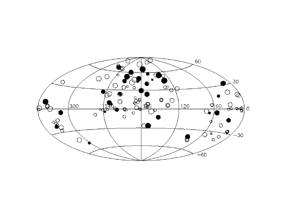
Figure 1.— Location of all 137 ChaMP high latitude ($|b|>20\deg$) fields is shown in an Aitoff equatorial projection, with RA and Dec in decimal degrees. Filled circles represent ACIS-I at the aimpoint, and open circles ACIS-S. The average area for ChaMP-selected ObsIDs corresponds to 5.8 CCDs turned on, each of which is 8.3′ on a side. Point size crudely indicates Chandra  exposure times, varying from 2 to 190 ksec.

The fields studied in this pilot paper include 6 early (Cycle 1) fields listed in Table 1 for which we have already reduced and calibrated both archival X-ray images and photometric NOAO 4 meter/Mosaic imaging. These 6 fields represent about 12% of ChaMP fields of similar exposure time or greater. Four of the 6 fields have clusters as their intended Chandra  targets. We do not include the intended (PI) targets in our analysis, their presence may bias the sample of source types analyzed here. The large number of fields in the full ChaMP and the variety of PI target types allow important tests for possible sample biases. While an excess of point sources in cluster fields has been claimed anecdotally (Cappi et al., 2001; Martini et al., 2002), no significant difference is found using the larger sample of Chandra images (29 with clusters and 33 without) in Kim et al. (2003b).

Table 1Chandra  Fields

ObsID	PI Target	Exposure	ACIS CCDs	RA	DEC	UT Date	Galactic $N_{H}$
		(ksec)		J2000			($10^{20}$cm-2)
536	MS1137.5+6625	114.6	012367	11:40:23.3	+66:08:42.0	1999 Sep 30	1.18
541	V1416$+$4446	29.8	01237	14:16:28.8	+44:46:40.8	1999 Dec 02	1.24
624	LP944$-$20	40.9	23678	03:39:34.7	$-$35:25:50.0	1999 Dec 15	1.44
861	Q2345$+$007	65.0	23678	23:48:19.6	+00:57:21.1	2000 Jun 27	3.81
914	CLJ0542$-$4100	48.7	01237	05:42:50.2	$-$41:00:06.9	2000 Jul 26	3.59
928	MS2137$-$2340	29.1	23678	21:40:12.7	$-$23:39:27.0	1999 Nov 18	3.57

3. X-ray Image Processing and Analysis

We have used Chandra archival data reprocessed (in April 2001) at CXC. The foundation of the ChaMP rests on our own Chandra  image analysis pipeline XPIPE (Kim et al., 2003a), built mainly with CIAO tools (http://asc.harvard.edu/ciao), and designed to uniformly and carefully screen and analyze the X-ray data. Details of XPIPE can be found in our X-ray companion paper, Kim et al. (2003a). Briefly, XPIPE screens high particle background periods, cosmic rays and hot pixels from each ACIS CCD exposure. Wavelet transform detection is performed (using wavdetect; Freeman et al. 2002) at 7 scales from 0.5 to 32″  thus accommodating the Chandra  PSF variation as a function of off-axis angle from the mirror axis. We select a significance threshold parameter of $10^{-6}$ per pixel, which corresponds to about one spurious pixel detection per CCD. We have confirmed this rate by an extensive simulation showing that the number of spurious sources detected is always less than this rate. An additional flux criterion of signal to noise ($\frac{S}{N}$) greater than 2 from our X-ray photometry further decreases the number of spurious sources in the sample. We avoid spurious sources near detector edges by generating an exposure map for each CCD with the appropriate aspect histogram, and then applying a minimum exposure threshold of 10% to all pixels included for analysis.

The absolute celestial positions of sources detected with wavdetect are accurate to about 1″, which is the specified absolute position accuracy for the Chandra observatory. To check for and minimize any systematic offset in the absolute source positions returned by wavdetect, the positions of X-ray sources are correlated to optical sources in the field. The average position offset from X-ray sources to matched optical sources is then applied to each X-ray source position. This procedure is described in more detail in §5.1.

We visually inspect all the X-ray images to validate sources and flag them for contamination (by hot pixels, readout streaks, bad bias values) or excessive uncertainty due to contamination of source or background regions. Throughout this paper and for ChaMP statistics, the target sources are flagged and excluded from analysis in all fields. Source catalogs and FITS images are being made publicly available, with details at the ChaMP web site, http://hea-www.harvard.edu/CHAMP/.

At the X-ray source positions derived from wavdetect, we perform aperture photometry. We use a circular source aperture whose radius encompasses 95% of deposited energy, determined at 1.5 keV, but restrict this radius to the range $3\arcsec<r_{ap}<40\arcsec$. We use a background annulus extending from 2 to 5 times $r_{ap}$, excluding flux within $r_{ap}$ of any other detected sources in the annulus. We perform photometry in 3 energy bands: soft ($S$; 0.3-2.5 keV), hard ($H$; 2.5-8 keV), and broad ($B$; 0.3-8 keV). We calculate net count rates using the effective exposure and vignetting factors both at the source and background regions.

Only sources with ${\frac{S}{N}}>2$ in at least one of the bands $B$, $S$, or $H$ are included for analysis here. Flux is calculated from the net count rate in the $B$, or if necessary from another ($H$ or $S$) band to satisfy our ${\frac{S}{N}}$ criterion. We assume a power-law of photon index $\Gamma=1.4$ absorbed by a neutral Galactic column density $N_{H}$ taken from Dickey & Lockman (1990) for the Chandra  aimpoint position on the sky. The effect of varying the source model between reasonable powerlaw slopes from $\Gamma=1.0$ to 2.5 causes (for ${N_{H}^{Gal}}=3\times 10^{20}$cm^-2) an increase in the derived $f_{X}$(0.5-2 keV) of $\sim 12\%$ for FI chips, and 6% for BI chips.

The input bandpass energy range is passed to PIMMS (Mukai 1993; v3.2d, which includes Chandra  Cycle 4 effective area curves) along with the adjusted count rate and spectral model parameters to calculate a de-absorbed flux $f_{X}$ in the 0.5-2 keV band, since this bandpass is most useful for comparison to numerous published results from ROSAT, XMM, and Chandra. The error in $f_{X}$ is computed by applying the same counts-to-flux conversion factor to the error in counts, increased by a further 15% to qualitatively account for errors induced by the spectral model assumptions. These results are listed on-line along with other quantities described below.

For every source, we wish to calculate an effective on-axis ACIS-I hardness ratio

$$HR=\frac{H-S}{H+S}$$

that may be fairly compared among sources to study their X-ray properties even in the low counts regime. Many (especially weak) sources have derived $H$ or $S$ counts that are formally $<2\sigma$, or even negative. Naive inclusion of these yields nonsensical $HR$ values outside the physical range from -1 to 1. Therefore, we first replace such counts by a $2\sigma$ upper limit. This yields for $HR$ either a ‘detection’ (when both $H$ and $S$ counts are $>2\sigma$), an upper limit (when $H<2\sigma_{H}$), a lower limit (when $S<2\sigma_{S}$), or very rarely an indeterminate value (both).

Mirror reflectance changes as a function of energy and of the angle $\theta$ between the source and Chandra’s aimpoint, causing energy-dependent vignetting. A different energy dependence arises from the detecting CCD - the quantum efficiency of backside- (BI) vs. frontside-illuminated (FI) chips. Therefore, for an identical source spectrum, different $HR$ values result, depending on $\theta$ and chip. To correct for this, we perform a second adjustment of $H$ and $S$ counts, normalizing them to refer uniformly to an on-axis source falling on an FI chip. To do this, we have modified the PIMMS code to include vignetting. Where the integration of source model is convolved with the instrument effective area (EA), we incorporate an extra multiplicative factor - the percentage of the on-axis EA as a function of photon energy and $\theta$. We interpolate between analytic fits (courtesy Diab Jerius) to EA as a function of $\theta$ from 0 to 30′, performed for 4 energies (0.49, 1, 1.48, 2.02, 2.99, and 6.4 keV). Similar curves are shown in the CXC Proposer’s Guide Rev4.0 (CXC v4.0, 2001).

To derive the corrected hardness ratio $HR_{0}$, we first convert counts to de-absorbed flux in each band using our standard source model, the source $\theta$ and chip. Using the same source model, we then convert the derived flux back counts at $\theta=0$ on an FI chip. The resulting corrections in $HR_{0}$ do not depend strongly on the assumed $\Gamma$; the difference in the mean $HR_{0}$ derived assuming $\Gamma=0.5$ and 3.0, is only 0.02 (3%) out to 15′  off-axis.

We have performed a series of simulations to derive the expected $HR_{0}$ values for high ${\frac{S}{N}}$ sources across a grid of $\Gamma$ and $N_{H}$ values, as shown in Figure 2. A comparison to the median corrected value of $\overline{HR_{0}}=-0.5$ for all sources detected in both $H$ and $S$, and assuming no absorption implies $\Gamma\sim 1.4$.

Finally, if at least one of $H$ and $S$ are significant, then we calculate errors for $HR_{0}$ from the $H$ and $S$ counts (or limits) as

$$\sigma_{HR}=\frac{2}{(H+S)^{2}}\sqrt{S^{2}\sigma^{2}_{H}+H^{2}\sigma^{2}_{S}}.$$

Figure 2.— Simulated on-axis FI chip Hardness Ratios for high ${\frac{S}{N}}$ sources. Top. The family of curves show the resulting $HR$ for different ($z=0$) absorbing columns as a function of power-law Photon Index $\Gamma$. Bottom. The family of curves show the resulting $HR$ for different values of power-law Photon Index $\Gamma$ as a function of absorbing column.

4. Optical Imaging

Optical imaging is crucial to provide optical fluxes, preliminary source classification, and accurate centroiding for spectroscopic followup. Optical centroids supersede X-ray centroids for extended or multiple objects, for cluster galaxies, or for Chandra  sources with large off-axis angles and hence less accurate X-ray positions. Multiband colors can provide source classifications and photometric redshifts for the majority of fainter ChaMP sources (${r^{\ast}}>22$) for which high quality spectra are more difficult to obtain.

4.1. Exposure Times

For every ChaMP field, we scale our optical exposure times to the Chandra  X-ray exposure times, to provide a uniform sensitivity to X-ray/optical flux ratios. Our color-limited survey thus minimizes optical telescope usage, while accessing for every field a similar fraction of every object type. To convert X-ray counts to flux, we first assume 80% of the exposure time remains after cleaning high particle background periods. The low background and small PSF of Chandra allows high confidence detection of point sources with as few as 4-5 photons, but to reduce uncertainties on $~{}f_{X}$  and thereby improve object class discrimination, we adopt 10 counts as the ChaMP minimum detection limit. We convert the detectable number of counts for each Chandra  field to an X-ray flux limit, and then scale the corresponding optical magnitude limit to include $>90\%$ of ROSAT AGN even at the X-ray flux limit, based on 1448 ROSAT-detected quasars from Yuan et al. (1998). The typical resulting magnitude limit as a function of Chandra  exposure time $T$ can be expressed as $V=14.17+2.5\,{\rm log}T$. This criterion (${\rm log}\frac{f_{X}}{f_{V}}<0.9$) should include larger fractions of other source types with brighter relative optical emission like stars and most galaxies. Sources that are relatively weak optically compared to ROSAT quasars will have a lower completeness and a brighter effective limiting magnitude in our survey (e.g., sources suffering from substantial optical extinction). Details of our optical imaging for these 6 fields are presented in Table 2. The resulting desired limits range from $V$ mags (note that $V\sim(g^{\prime}+r^{\prime})/2$) of 21 to 26 with a median of 23.5 mag for all ChaMP fields. However, to achieve reasonable limits on the amount of required optical imaging time, we limit our maximum desired optical magnitude limit to $V\sim 25$ in any field.

Table 2Optical Imaging

ObsID	E(B-V)	Telescope	UT Date	Filter	Dithers	Exposure	Airmass	FWHM	mTO	m5σ
						(total sec)	(Mean)	(″)	Limit	Limit
536	0.0131	KPNO 4m	12 Jun 2000	$g^{\prime}$	2	1200	1.39	2.2	22.875	23.9
				$r^{\prime}$	2	1200	1.43	2.0	22.875	24.2
				$i^{\prime}$	2	1200	1.48	1.9	22.625	23.8
541	0.008	KPNO 4m	12 Jun 2000	$g^{\prime}$	2	1000	1.33	1.9	22.875	23.9
				$r^{\prime}$	1	500	1.40	2.0	22.125	23.7
				$i^{\prime}$	1	500	1.50	1.7	22.125	23.5
624	0.014	CTIO 4m	28 Sep 2000	$g^{\prime}$	3	810	1.05	1.2	24.875	25.9
				$r^{\prime}$	3	630	1.01	1.1	24.125	25.3
				$i^{\prime}$	3	720	1.00	1.1	23.375	24.4
861	0.0246	CTIO 4m	28 Sep 2000	$g^{\prime}$	3	1260	1.23	1.4	24.625	25.8
				$r^{\prime}$	3	1080	1.17	1.4	24.375	25.3
				$i^{\prime}$	3	1170	1.17	1.1	23.375	24.3
914	0.0383	CTIO 4m	28 Sep 2000	$g^{\prime}$	3	990	1.04	1.2	25.125	26.1
				$r^{\prime}$	3	810	1.06	1.2	24.375	25.4
				$i^{\prime}$	3	900	1.09	1.2	23.375	24.2
928	0.051	CTIO 4m	28 Sep 2000	$g^{\prime}$	3	900	1.01	1.6	24.375	25.6
				$r^{\prime}$	3	720	1.02	1.3	24.125	25.2
				$i^{\prime}$	3	810	1.05	1.0	23.375	24.3

NOAO 4-meter imaging with the Mosaic CCD cameras (Muller et al., 1998) is key to the ChaMP, since it provides adequate depth, spatial resolution ($\sim 0.26\arcsec$/pixel), and a large field of view ($36\arcmin\times 36\arcmin$) over the full Chandra  FoV. For shallower northern fields, for secondary calibration of deep imaging from non-photometric 4 meter (4m) nights, and for imaging bright objects within deep fields, the ChaMP also uses the FLWO 1.2m with the 4shooter CCD on Mt Hopkins ($0.32\arcsec$/pixel, 22′  field). In this paper, we report only deep 4m fields observed in photometric conditions.

We dither the 4m/Mosaic pointings to allow for better sky flat construction, averaging over defects, cosmic ray removal, and gap coverage. While the optical data reduction is conceptually straightforward, it is in practice complicated by the size of the data set (285 MB per image), and by the need to interactively manage bad pixel flagging. After photometric analysis, our final reduced images are stored in (short) integer format, which reduces their size by a factor of two, with $<1\%$ effect on measured magnitudes.

4.2. Filter Choice

The ChaMP uses Sloan Digital Sky Survey (SDSS) $g^{\prime}$, $r^{\prime}$, and $i^{\prime}$ filters (Fukugita et al., 1996), whose steep transmission cutoffs improve object classification and photometric redshift determination (Gonzalez & Maccarone, 2002; Richards et al., 2001). While $\frac{f_{X}}{f_{opt}}$  is clearly our primary discriminant of AGN from stars, at least 2 optical filters are required to also constrain stellar spectral class. Still, with just 2 filters, high-z, reddened or obscured AGN may share the stellar locus with M dwarfs (Lenz et al., 1998), so we chose 3 filters to separate such quasars from stars because these types of AGN represent a prime science goal of the ChaMP. Furthermore, it has already been demonstrated that AGN of redshift $3.5<z<5$ can be constrained to $\Delta z\sim 0.2$ with SDSS $g^{\prime},r^{\prime},$ and $i^{\prime}$ colors (Richards et al., 2001). Since $g^{\prime}$ and $r^{\prime}$ also bracket the 4000Å  break in $z>0.8$ cluster ellipticals, this aids distance estimation and cluster membership evaluation. The bright $\lambda 5577$ night sky line falls between the $g^{\prime}$ and $r^{\prime}$ filters, allowing fainter limits to be achieved in shorter integration times. Finally, someday the need for NOAO northern imaging followup will be relieved by the SDSS itself for the shallower ChaMP fields. The huge database of SDSS magnitudes and colors help with deeper fields and core science as well by offering (1) bootstrap calibration of deep ChaMP imaging observed in non-photometric conditions (2) calibration and testing of accurate photometric redshifts (Richards et al., 2001) and source classification (Newberg, 1999) (3) detailed comparisons between SDSS optical and ChaMP X-ray sample selection.

4.3. Optical Image Reduction

The reduction of the raw optical CCD images is primarily done using standard techniques in IRAF. The Mosaic cameras utilize the multi-extension FITS format, allowing the eight individual CCD images to be treated as a single image for most reduction purposes. The IRAF package mscred (Valdes, 2002) is used to properly handle the multi-extension FITS images and to simplify the data reduction. Although an overview is presented here, a detailed reduction walkthrough is available for the NOAO Deep Wide Field Survey (NDWFS) data (Jannuzi & Dey, 1999) using the same instruments.

Standard calibration images are taken at the telescope (bias, dome flats, etc.) excluding twilight sky flats. We construct a master super-sky flat by combining multiple object frames, thereby rejecting real objects in the frame and leaving us with a high ${\frac{S}{N}}$ image of “blank” sky. These improve the flat-field correction provided by conventional dome flats, mostly by accounting for differences in each filter between the night-sky and our dome lamp color. Before the super-sky flat can be made, images from the KPNO 4m also require subtraction of a pupil ghost caused by light back-scattered from the telescope optics, which affects primarily the inner four CCDs. Because the pupil ghost changes with the amount of light entering the telescope, its strength varies with the filter used, and with ambient light from the moon or bright stars near the field of view. For this reason we create a template pupil ghost seperately for each filter, taking care to exclude images with extremely bright saturated objects near the center of the field of view. Once a template pupil has been generated, it must be scaled and subtracted from individual object frames in each filter, a process that is now largely automated.

4.4. Astrometry and Photometry

We first derive ($\sim 0.3\arcsec$ RMS) astrometry from our optical imaging to enable accurate X-ray source matches, and optimal positioning of spectroscopic fibers or slits. The (J2000) position of the optical sources are referenced to the Guide Star Catalog II. Final positions used by the ChaMP for all matched sources are the average of positions measured from all optical filters in which an object is detected.

We use SExtractor (Bertin & Arnouts, 1996) to detect sources, and measure their positions and magnitudes. A first run of SExtractor is used to measure the mode $\Gamma$ of the FWHM of stellar objects in each image. For this step, our filters first remove objects that are unreliable (any with processing error flag $>3$ – cosmic rays, spurious blended, or contaminated sources, or sources near a chip edge), sources that are too faint (typically $<2\times 10^{4}$ net counts) or too bright (typically $>2\times 10^{5}$ counts), and extended sources (SExtractor stellarity $<$ median). For program fields, we typically use a minimum detection threshold (SExtractor detect_thresh) of $0.8\sigma$ above background per pixel, and require a minimum grouping (detect_minarea) of $\Gamma^{2}/4$ pixels at this threshold for a detection. Since we are cross-correlating to X-ray sources - rare on the sky compared to optical sources - we are somewhat more concerned with completeness than with spurious source rejection. From detailed comparisons of dithered and deep stacked images of the same fields, we find that these parameter settings forge a good compromise between detecting most real sources, but not too many spurious sources.

A second run of SExtractor measures 3 instrumental magnitudes: one from a circular aperture with diameter FWHM (for highest ${\frac{S}{N}}$; see Howell et al. 1989), another with 4 times the FWHM (which we find encompasses 95% flux for point sources), and finally SExtractor’s mag_auto. The latter is a elliptical aperture magnitude (alà Kron 1980) that is robust to seeing variations, as described in Nonino et al. (1999). Following the convention of the early data release of the SDSS quasar catalog (Schneider et al., 2002), we present the optical photometry here as $g^{\ast}$, $r^{\ast}$ and $i^{\ast}$ since the SDSS photometry system is not yet finalized and the NOAO filters are not a perfect match to the SDSS filters. Standard stars calibrated for the SDSS are available from Smith et al. (2002) but are generally too few per field to practically allow for a complete photometric calibration, especially given the long readout times for the Mosaic. To facilitate the use of the many standard stars listed by Landolt (1992), we transform them to the SDSS photometric system using Fukugita et al. (1996) to derive our nightly photometric solutions. In the standard star fields, we find standard stars automatically by positional matching of accurate coordinates for Landolt standards (Henden, 2002) to SExtractor source positions, using a high ($\sim 7\sigma$) SExtractor detection threshold to provide unambiguous detections.

We merge instrumental photometry results from each filter into a multicolor file by positional matching using a search radius of 1″. If multiple matches are found within this radius, the closest match is retained. If no matching detection is found in some filter, the RMS of the background for that filter at that object’s position is recorded for later conversion to a limiting magnitude. In these 6 fields, our merged catalog of Mosaic photometry contains about 343,000 objects with flags $<4$ indicating good photometry in at least one band.

We then perform photometric calibration of the standard stars for each night via a 2-step multilinear method (Hardie, 1962), adapted from an implementation written in IDL by James Higdon. For a given night, for the instrumental magnitude $v$ in each filter, we solve the linear equation

$$v_{0}-v=(k_{0}+k_{1}X)+e(c_{0})+z$$

where $v_{0}$ and $c_{0}$ are the standard star’s cataloged magnitude and color, respectively, $e$ the color coefficient, $z$ a zeropoint correction, and $k_{0}$ and $k_{1}$ are extinction coefficients. We iteratively solve for these 4 coefficients, first freezing $k_{0}$ and $k_{1}$ and solving for $e$ and $z$, then freezing $e$ and $z$ and solving for $k_{0}$ and $k_{1}$, until the solution converges (typically 3 or 4 iterations). We then delete measurements with residuals exceeding $3\sigma$, and repeat the solution until no such residuals remain.

Similarly, for each color $c$ we iteratively solve the linear equation

$$c_{0}=e(c+k_{0}+k_{1}X)+z$$

for the four coefficients $e,z,k_{0}$ and $k_{1}$, deleting measurements with residuals exceeding $3\sigma$ as before. We tested the final results from our procedure against that of Harris, Fitzgerald, & Reed (1981) as implemented in the IRAF photcal procedure, and find results identical to within the errors. Our calibrations produce $e,z,k0,k1$ coefficients for each of $g^{\ast}$, $r^{\ast}$, $i^{\ast}$, $(g^{\ast}-r^{\ast})$, and $(r^{\ast}-i^{\ast})$. Since these calibrations for these NOAO filters have not been published previously, we list them in Table 3 as a reference. The final transformations are applied to the standard stars to derive RMS residuals for each night for $g^{\ast}$, $r^{\ast}$, $i^{\ast}$, $(g^{\ast}-r^{\ast})$, and $(r^{\ast}-i^{\ast})$. These are listed in Table 3 for each night. The nightly transformations applied to our program objects are

$$c^{\ast}=e(c+k_{0}+k_{1}X)+z$$

$$v^{\ast}=v+(k_{0}+k_{1}X)+e(c\prime)+z$$

where $c^{\ast}$ and $v^{\ast}$ are the final calibrated color and magnitude, respectively.

Table 3Nightly Photometric Calibration Coefficients

Fit Variable	$e$	$z$	$k_{0}$	$k_{1}$	N Stars	Fit RMS
	(mag)					(mag)
KPNO 4m 12 June 2000
$g^{\ast}$	0.060	25.314	0.284	-0.217	52	0.057
$r^{\ast}$	-0.055	25.424	0.207	-0.155	49	0.068
$i^{\ast}$	-0.185	25.194	0.191	-0.117	54	0.250
$g^{\ast}$–$r^{\ast}$	1.021	-0.087	0.044	-0.036	54	0.111
$r^{\ast}$–$i^{\ast}$	0.978	0.362	0.064	-0.050	47	0.031
CTIO 4m 28 September 2000
$g^{\ast}$	0.038	25.695	0.257	-0.210	43	0.027
$r^{\ast}$	-0.020	25.794	0.145	-0.118	43	0.033
$i^{\ast}$	0.083	25.358	0.089	-0.072	41	0.041
$g^{\ast}$–$r^{\ast}$	1.011	-0.087	0.110	-0.090	41	0.037
$r^{\ast}$–$i^{\ast}$	0.903	0.410	0.078	-0.064	43	0.027

For objects not detected in any optical filter, we assign a magnitude limit $m_{5\sigma}$ corresponding to a flux of $5\sigma$ detection where $\sigma$ is the background RMS at that position. Starting from the standard CCD equation, we find

$$m_{D\sigma}=-2.5\,{\rm log}\Bigl{(}\frac{D~{}\Gamma~{}\sigma}{T}\Bigr{)}+z$$

Here, $D$ is the desired $\frac{S}{N}$. The RMS noise at the position of an object on the CCD is denoted as $\sigma$; $\Gamma$ is again the FWHM in pixels, $T$ is the total exposure time, and $z$ indicates that the photometric calibration is applied, for which we assume the mean color for objects in the field. This limiting point source magnitude is listed for each field in Table 2 for the median background RMS in the field. Objects at these magnitudes are not detected with high completeness. From our comparisons of individual dithered and deep stacked images, we find that the magnitude where the number counts peak in a differential (0.25 mag bin) number counts histogram corresponds approximately to 90% completeness in the magnitude range 20 – 25. This turnover magnitude $m_{\rm TO}$ is typically about 1 mag brighter than the $5\sigma$ limiting magnitude. Both magnitude limits are listed in Table 2.

We perform several sanity checks on the final photometry. First, we plot color-color diagrams against a crude mean stellar locus from the SDSS Early Data Release (EDR). The locus we derive by eye (from objects with $<0.1$mag error among 30,000 high latitude objects) in the SDSS EDR corresponds to one line primarily following the SDSS halo/thick disk locus (Chen, 2001; Yasuda et al., 2001)

$${(r^{\ast}-i^{\ast})}\sim 0.4029{(g^{\ast}-r^{\ast})}-0.007$$

and another following the thin disk locus

$${(r^{\ast}-i^{\ast})}\sim 14.286{(g^{\ast}-r^{\ast})}-18.5$$

An example of these color loci is shown in Figure 10, to be discussed in more detail in § 7.3. By studying a variety of SDSS fields at 7 different galactic latitudes ($b=$ 30, 35, 45, 60, –45, –55, –65) we find variations of about 0.2mag in $(r^{\prime}-i^{\prime})$ occur in the thin disk locus.

We also compare our magnitudes in $g^{\ast}$  and $r^{\ast}$  to magnitudes derived from the GSC2.2. We have derived the transformation between SDSS EDR and GSC2.2 magnitudes by direct comparison of the two surveys, using only stars between 17th and 19th magnitude. After $3\sigma$ clipping, the typical residuals are 0.2 mag, with zeropoints differing by $\sim 1\%$.

$${g^{\ast}}=1.032\,J+0.1255(J-F)-0.851$$

$${r^{\ast}}=0.982\,F+0.1518(J-F)+0.451$$

$${i^{\ast}}=0.994\,F-0.1235(J-F)+0.281$$

We note that most optical point sources brighter than 18th mag suffer from saturation effects in our NOAO 4m imaging. While these objects constitute a small fraction ($\sim 6\%$) of our optically identified X-ray sources, they are a larger fraction ($\sim 10\%$) of our spectroscopically-classified objects. We expect a full release of the SDSS will substantially alleviate this problem, as will our ongoing imaging study of these fields with the SAO FLWO1.2m and 4-shooter CCD on Mt Hopkins.

Since most of our X-ray sources are extragalactic, before calculations of optical luminosities, we correct the optical magnitude measurements for Galactic extinction using the maps of Schlegel, Finkbeiner, & Davis (1998). We assume an $R_{V}=3.1$ absorbing medium, and absorption in the SDSS bands as given by Schneider et al. (2002).

5. X-ray to Optical Source Matching

For the ChaMP, Kim et al. (2003a) have carried out extensive simulations of point sources generated using the SAOSAC raytrace program (http://hea-www.harvard.edu/MST/) and detected using CIAO/wavdetect (Freeman et al. 2002). For weak sources of $\sim 20$ counts between 8-10′  off-axis from the aim point, the reported X-ray centroid position is correct within $1.8\arcsec$, corresponding to a $1\sigma$ confidence contour.

The source naming convention of the ChaMP as officially registered with the IAU is given with a prefix CXOMP (Chandra X-ray Observatory Multiwavelength Project) and affixed with the truncated J2000 position of the X-ray source (CXOMP Jhhmmss.s$\pm$ddmmss) after a mean field offset correction is applied, derived from the positional matching of optical and X-ray sources in each field.

5.1. Matching criteria

5.1.1 Automated Matching

We obtain candidate optical identifications of X-ray sources in each field using a 2-stage automated position matching process between optical and X-ray source positions. In the first stage, the subset of X-ray sources within 5′ of the Chandra aimpoint and with X-ray $B$ (0.3–8 keV) detections $>20$ counts are matched to optical sources from our CCD imaging, using position matching with a radial offset matching tolerance, in arcsec, $R_{\rm match}=\theta/\log_{10}(B)$, where $\theta$ is the off-axis angle in arcminutes, and $B$ is the X-ray source counts, but $R_{\rm match}$ is limited to a minimum of 3″ for all sources. This matching tolerance encompasses the wavdetect centroid positional uncertainty variation with off-axis angle and source counts, using the refined source position estimator described in Kim et al. (2003a). The optical position errors are neglegible in comparision. In those cases where there are multiple optical matches, the closest match is used. The median X-ray to optical position translational offset of these matched sources is then applied to all the X-ray sources for the field, to bring the optical and X-ray source lists onto the same coordinate frame. The X-ray position corrections are typically less than 1″, which is consistent with the specified absolute position accuracy for the Chandra observatory and wavdetect source positions. Figure 3 shows optical matches overlaid directly on the ACIS-I image of ObsID 536.

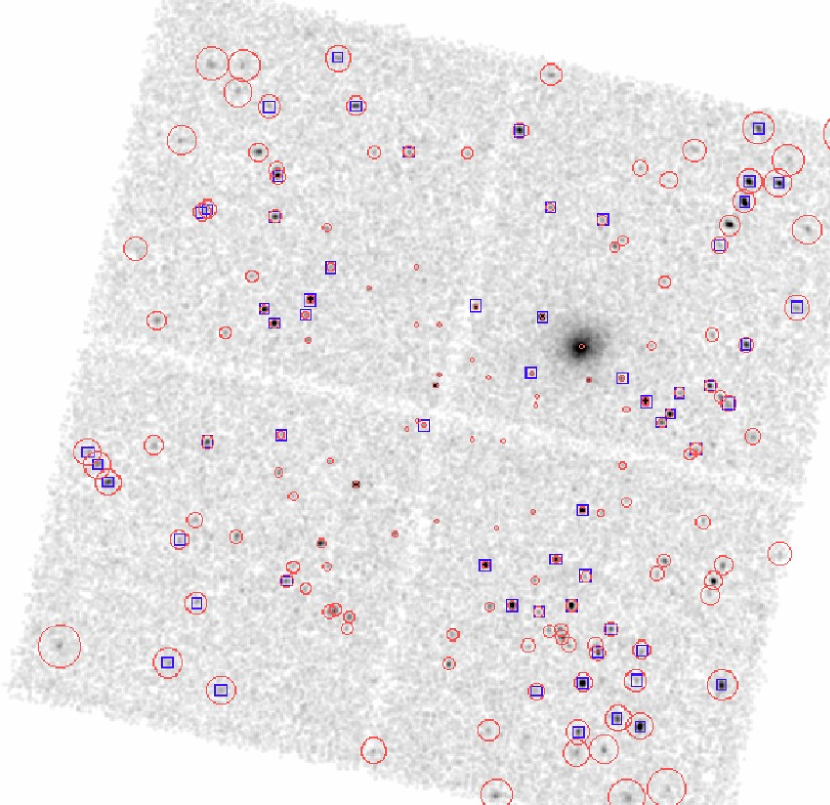
Figure 3.— Chandra  image of the field of ObsID 536 (target MS1137.5+6625). The $16\arcmin\times 16\arcmin$ ACIS-I (0.3-5 keV) image (N up, E to the left as in all images) was smoothed with a 3 pixel (1.5$\arcsec$) gaussian for clarity. 156 X-ray sources detected to $2\times 10^{-16}~{}{\rm erg~{}cm}^{-2}~{}{\rm s}^{-1}$ using the ChaMP’s X-ray pipeline are marked with circles sized to the Chandra  PSF (90% EE). To the 125 ${\frac{S}{N}}>2$ X-ray sources detected in these 4 chips, we have matched 80 optical sources detected in our combined 4m/Mosaic images to ${r^{\ast}}\sim 25$, indicated by 15″ boxes. The target cluster is easily visible as the extended source NW of center, and is detected as a single source by XPIPE, but like all target objects is excluded from ChaMP analysis.

In the second stage of position matching, optical matching is performed for all X-ray sources with X-ray $B$ detections $>5$ counts, using the same matching tolerance $R_{\rm match}$ as above. Multiple optical matches for an X-ray source are allowed in this stage, and are passed to the visual inspection process described next. Extended X-ray source centroids may have larger position errors than are predicted by our point source formula. Furthermore, in some cases no corresponding optical cluster galaxy may exist close to the cluster X-ray centroid. If no optical counterpart is found in the automated matching routine for these or other cases, visual inspection provides a second chance to identify counterparts.

5.1.2 Visual Inspection

After our automated O/X matching between detected sources from XPIPE and SExtractor source positions has been performed, we examine the images by eye. An example of the plots used for visual inspection is shown in Fig 4. In many cases, no obvious optical counterpart can be detected, while in other cases there are several (source confusion). Even with typical astrometric accuracy of an arcsec, at these faint optical magnitudes and X-ray fluxes we frequently find several optical counterpart candidates. Beyond ${r^{\ast}}\sim 20$, galaxies dominate the optical number counts, and at by 24th magnitude, cumulative source counts are near $10^{5}\,$deg^-2 (Kümmel & Wagner, 2001). At these faint magnitudes, the probability of finding an unrelated optical source by chance within any 3″  circle becomes $\sim 20\%$. The small PSF and accurate centroiding of Chandra  become crucial at these faint magnitudes, as does careful source inspection.

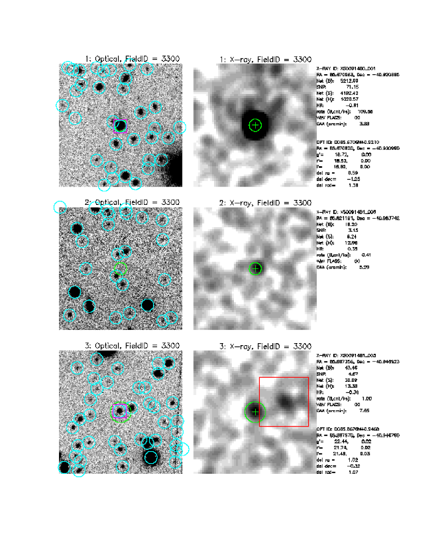
Figure 4.— An example from ObsID 914 (target CL J0542.8-4100) of the pages used for initial visual inspection of X-ray source matches. RIGHT PANELS: A 1′  field centered on a detected X-ray source is shown, with N up and E to the left. The 0.3-8  keV X-ray image is smoothed with a 2 pixel (1$\arcsec$) gaussian for clarity, which facilitates source inspection and examination of background and confusion effects. Green circles around the X-ray source have size equal to the PSF (50% EE) at the source position. Crosses show the wavdetect X-ray centroid. If other X-ray sources are detected within the field, they are marked by a 20″  box. LEFT PANELS: The corresponding optical $r^{\ast}$  images shows all optical sources detected by SExtractor, marked with $3\arcsec$ circles. The Chandra 50% EE circle is reproduced at the X-ray source position. When our automated matching procedure finds an optical counterpart, the optical source is marked with a 3″  box. X-ray and optical photometric data are displayed to the far right.

5.2. Fraction with Optical Counterparts

During visual inspection of the optical field of each X-ray source, we assign a match confidence to each plausible counterpart. To consider a sample as uncontaminated as possible by incorrect matches, we have removed from further optical analysis below 45 X-ray sources with poor or ambiguous counterpart assignments.

The resulting fraction of X-ray sources with confidently matched optical counterparts is shown in Table 4. We have not yet achieved the desired optical magnitude limits (set to match optical counterparts for 90% of ROSAT AGN) in all these deep Chandra  fields, but the imaging has served to facilitate spectroscopy to ${r^{\ast}}\sim 21$, and to provide fluxes and colors to still deeper limits. Lower achieved match fractions also reflect the inclusion by Chandra of new $\frac{f_{X}}{f_{opt}}$ populations atypical for ROSAT such as heavily absorbed AGN.

Table 4Source Matching

ObsID	$N_{X}$	$N_{XO}$	$f_{XO}$	$N_{XOS}$	$f_{XOS}$
			%		%
536	140	77	55	33	70
541	65	45	69	24	72
624	58	45	78	19	74
861	80	57	71	14	59
914	88	65	74	20	50
928	55	42	76	15	50
Total	486	331	71	125	63

Excluding the $\sim 10\%$ of sources with more than 200 X-ray counts, the mean/median X-ray flux for matched sources (3.5/2.4 in units of 10^-15  erg cm^-2 s^-1) exceeds the flux for unmatched sources (2.6/1.6) as expected, but not strongly. The mean off-axis angle of unmatched sources ($\theta=6.7\pm 3.9$′) is indistinguishable from that of matched sources ($6.2\pm 3.2$′; both quoted errors are 1$\sigma$ RMS).

For a typical ChaMP source in these fields, the median X-ray (0.5 - 2 keV) flux is $2.4\times 10^{-15}$  erg cm^-2 s^-1, where according to the logN-logS, the cumulative (0.5-2 keV) X-ray source density attains about 30deg^-2 (e.g., Rosati et al. (2002)). The probability of two X-ray sources falling within 10″  of each other by chance is $<0.001$. On the other hand, the number of true multiple sources is of great interest; they may either be lensed images or perhaps binary AGN, possibly interaction-triggered (e.g., Green et al. 2002). Since these latter types are expected to be rare, a large-area survey like the ChaMP is needed to find them. New close pairs of X-ray sources with optical counterparts are described in Appendix A.

6. Optical Spectroscopy

The nature of many individual sources, especially those with unusual properties, cannot be reliably determined until spectroscopy is obtained. Our spectroscopy targets all objects in a representative subset of 40 ChaMP Cycle1+2 fields, yielding $\sim 1000$ objects for which we will obtain the most detailed information. With our spectroscopic subsample, we will classify sources by type, determine redshifts and hence luminosities and look-back times for evolutionary studies, and test photometric determinations of redshift and classification.

The mean magnitude of optical counterparts is $r^{\prime}\sim 22$ for a 23 ksec high galactic latitude Chandra  exposure, and so fields of this Chandra  exposure or larger typically have at least 15 sources suitable for fiber spectroscopy. Multi-fiber spectroscopy, even on 4 to 6m telescopes, allows us to consistently obtain source classification and redshifts to $r^{\prime}\sim 20$, and up to 1.5mag fainter for objects with strong emission lines. Our overall spectroscopic observing strategy has been to use single-slit (FLWO1.5m w/ FAST) spectroscopy for isolated $r^{\prime}<17$ sources in shallow Chandra  fields, and in our deeper fields, which might otherwise introduce scattered light problems for multi-object spectroscopy. Multi-fiber wide-field spectroscopy with the HYDRA spectrographs (Barden, 1994) on the WIYN 3.5m and CTIO 4m telescopes enables us to acquire spectra for sources with $17<r^{\prime}<$21. A subset of faint ChaMP sources ($21<r^{\prime}<$23) in fields designated for spectroscopic follow-up are being observed with 6m class telescopes such as Magellan and the MMT. Table 5 lists the technical specifications and configurations for each spectroscopic facility used for results presented herein.

Table 5Spectroscopic Facilities

Telescope	Instrument	Mode	Grating/Grism	$\lambda$ range	R	Spectral
				(Å)	($\lambda/\Delta\lambda$)	Resolution (Å)
WIYN	HYDRA/RBS	multi-fiber	316@7.0	4500-9000	950	7.8
CTIO Blanco 4m	HYDRA	multi-fiber	KPGL3	4600-7400	1300	4.6
MMT	Blue Channnel	single slit	300 l/mm	3500-8300	800	8.8
Magellan	Boller & Chivens	single slit	1200 l/mm	4200-5800	2083	2.4
Magellan	LDSS-2	single slit	med/red	4000-8500	520	13.5
Keck	LRIS	multi slit	300 l/mm	4000-9000
FLWO 1.5m	FAST	single slit	300 l/mm	3600-7500	850	5.9

Of the 6 fields studied here, each has been observed with a multi-fiber spectrograph on either the WIYN or CTIO 4m through 2″ fibers (Table 6). An average of 15 spectra per field are acquired with this configuration. We obtained multi-slit observations for 17 sources with Keck-I/LRIS or Magellan/LDSS2. Single slit observations of 19 sources were acquired with the FLWO 1.5m when optically bright (${r^{\ast}}<17$) and MMT or Magellan when faint. We perform standard optical spectroscopic reductions within the IRAF environment. For multi-fiber reductions, we use the IRAF task dohydra. To optimize sky subtraction, we cross-correlated all dispersion-corrected (wavelength calibrated) sky spectra from random sky locations in the field against the object+sky spectrum from each object fiber using the task xcsao within the external IRAF package rvsao. We then median-combine the 9 sky fibers whose spectra correlate most closely with the total object+sky spectrum. We found this method to be superior to removal of a simple field-averaged sky spectrum for faint objects. Slit spectra were reduced using the IRAF task apall with a background signal measured locally for each object within the same slit. The multi-fiber spectra are only nominally flux-calibrated, since we use just 1 or 2 standards per night down a single central fiber. One or two standards are used for the single slit spectra.

Table 6Optical Spectroscopy

ObsID	Telescope	Instrument	UT Date	# of spectra
536	Keck	LRIS	15 May 2000	5
	WIYN	HYDRA	07 Apr 2001	7
	WIYN	HYDRA	30 Jan 2003	13
	WIYN	HYDRA	31 Jan 2003	4
541	WIYN	HYDRA	02 Apr 2001	12
	WIYN	HYDRA	07 Apr 2001	9
	MMT	Blue Channel	26 May 2001	1
	MMT	Blue channel	12 July 2002	2
624	CTIO 4m	HYDRA	16 Oct 2001	11
	Magellan	LDSS-2	03 Dec 2002	5
861	WIYN	HYDRA	19 Sep 2001	10
	WIYN	HYDRA	20 Sep 2001	2
	MMT	Blue channel	11 July 2002	1
	FLWO 1.5m	FAST	15 Oct 2001	2
914	CTIO 4m	HYDRA	17 Oct 2001	15
	Magellan	LDSS-2	01 Dec 2002	5
928	CTIO 4m	HYDRA	15 Oct 2001	7
	Magellan	LDSS-2	21 May 2001	1
	Magellan	BSC	15 July 2002	5
	Magellan	BSC	15 July 2002	1

6.1. Object types & Redshifts

We classify objects spectroscopically simply as broad line AGN (BLAGN; FWHM$>1000~{}{\rm km~{}s}^{-1}$) narrow emission line galaxy (NELG; FWHM$<1000~{}{\rm km~{}s}^{-1}$; some of which may be AGN), absorption line galaxy (ALG), or Star. Objects with high $\frac{S}{N}$ ($>20$) and no identifying features are denoted as BL Lac candidates, as are those whose identified CaII 4000Å  region shows a break contrast of $<0.25$ (see § 7.4.3). Our classification confidence level is denoted as well (0 for not classifiable, 1 insecure, 2 secure). These are all strictly optical classifications.

Redshifts are measured for extragalactic objects using the radial velocity package rvsao under the IRAF environment. This method depends on the optical classification. Quasar spectra are quite similar over a broad range of redshifts and luminosities (Forster et al., 2001), so that - absent the effects of broad absorption lines (BALs) or a strong Ly$\alpha$ forest absorption - a single high ${\frac{S}{N}}$ composite serves well as a redshift template. For BLAGN, we use the quasar template created from over 2200 quasar spectra collected by the SDSS (Berk et al., 2001). We run xcsao over the full redshift range in 0.1 redshift intervals, choosing the strongest correlation as the true redshift. Since the correlation strength depends strongly on ${\frac{S}{N}}$ and artifacts such as poorly subtracted sky lines, we inspect and visually verify all redshifts and classifications by comparison with overplotted templates. For ALG we use xcsao with a synthetic absorption line template. Whenever narrow emission lines are present, we elect to measure the redshift from these features to reduce the associated error. For NELG, the task emsao is used to identify emission lines using a line list. For stars, we assume an effective radial velocity of zero and allow xcsao to correlate against stellar template spectra from Jacoby, Hunter, & Christian (1984). Our comparisons between by-eye classifications and these automated results suggest an uncertainty of about one full spectral type.

For X-ray sources with ${r^{\ast}}<22$ optical counterparts, we have already achieved 54% completeness. All sources with $r>21$ that we have identified spectroscopically to date are BLAGN or NELG, because their strong emission lines facilitate classification and redshift determination. We are currently extending to 90% completeness at ${r^{\ast}}=21$ in at least 20 ChaMP fields specifically to map the space density of X-S AGN.

7. Results

7.1. Fluxes, Redshifts, and Object Types

Figure 5 shows a plot of the $r^{\ast}$  band magnitude against log$~{}f_{X}$  calculated in the 0.5–2  keV band. Overplotted are 3 lines of constant $\frac{f_{X}}{f_{r}}$  at 10, 1, and 0.1. We calculate this X-ray to optical flux ratio similarly to Hornschemeier et al. (2001) or Manners et al. (2002), using our SDSS $r^{\ast}$  magnitudes:

$${\rm log}\frac{f_{X}}{f_{r}}={\rm log}f_{X}+5.67+0.4\,{r^{\ast}}$$

and use this as our measure of $\frac{f_{X}}{f_{opt}}$ throughout. For comparison, we also plot a line showing the typical relation expected for O-S quasars (Green et al., 1995), assuming a constant ${\alpha_{ox}}=1.5$, which corresponds to ${\rm log}\,\frac{f_{X}}{f_{r}}=-0.57$. ChaMP quasars clearly differ from O-S quasars in the expected sense - X-S objects have typically stronger X-ray emission relative to optical ($\overline{{\rm log}\,\frac{f_{X}}{f_{r}}}=-0.15$). Alternatively, even optically ’dull’ quasars are still detected by the ChaMP, since luminous X-ray emission is the primary signature of AGN activity. BLAGN are X-ray bright, being largely limited to $\frac{f_{X}}{f_{r}}>0.1$. Galaxies tend to appear towards fainter X-ray fluxes but span a wide range of optical brightness. Stars are essentially limited to $\frac{f_{X}}{f_{r}}<0.1$ and ${r^{\ast}}<20$, which corresponds to a typical M dwarf at distances of $400-1000$ pc.

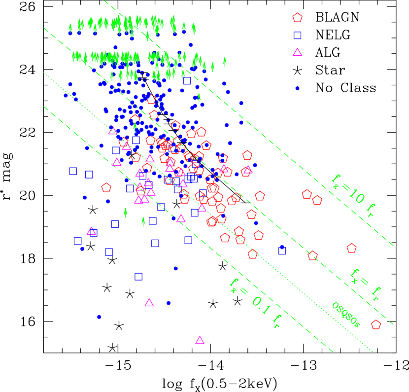
Figure 5.— SDSS $r^{\ast}$  band magnitudes vs. Chandra  log$~{}f_{X}$  (calculated for the 0.5–2  keV band from the broadband 0.3 - 8 keV counts) for all X-ray sources in the 6 fields studied here. Overplotted are 3 dashed lines of constant $\frac{f_{X}}{f_{r}}$  at 0.1, 1, and 10 calculated as described in § 7.1. A fourth (dotted) line marked OSQSOs shows the typical mean values for optically-selected quasars (${\rm log}\,\frac{f_{X}}{f_{r}}=-0.57$). Large symbols for different optical source types are shown as determined from our spectroscopy: broad line AGN (BLAGN), narrow emission line galaxies (NELG), absorption line galaxies (ALG) and stars. Any X-ray source not detected in our $r^{\ast}$-band images is marked with an arrow at the position of its $r^{\ast}$ magnitude limit. Small filled circles indicate sources with an optical counterpart in at least one filter. The curve traces the mean expected quasar track for $z=0.5$ redshift bins for the simulation described in § 7, imposed flux limits of ${\rm log}~{}f_{X}=-15$ and ${r^{\ast}}=25$. The bright end point has $\overline{z}=0.37$, while the faint end has $\overline{z}=4.6.$ Many of the optically faint objects are likely to be high$-z$ AGN. Magnitudes of point sources brighter than 18 suffer from saturation effects.

Apparent trends between fluxes or colors in any survey can be due to a combination of survey sensitivity limits. To investigate selection effects in a first approximation, we have generated a very deep simulated SDSS quasar catalog as described in (Fan, X., 1999), based on their observed optical luminosity function and its evolution, and including the effects of emission lines and intervening absorption. We have extended the simulation to include AGN with $M_{B}<-21$ out to a redshift of 6, corresponding to ${z^{\prime}}$ magnitudes to 28. We then assume that the mean observed ratio ${\rm log}\,\frac{f_{X}}{f_{r}}$  has a constant value of –0.14 with a dispersion $\sigma_{xr}=0.4$. (These are the actual values we find for all 41 quasars in our sample in the flux regime $f_{X}>5\times 10^{-15}$ erg cm^-2 s^-1 where our optical matching rate is high.) From the ${r^{\prime}}$ mag for each simulated quasar, we then generate X-ray fluxes, luminosities, etc. Finally, we can cut the sample at any desired mag or X-ray flux. Primarily, we use a cut of ${r^{\prime}}<25$ and ${\rm log}~{}f_{X}=-15$, similar to our actual final sample limits. For most figures which require redshifts, we use a cut of ${r^{\prime}}<22$ more appropriate to the spectroscopic sample. The simulated sample is thus based on a quasar OLF with an assumed constant observed $\frac{f_{X}}{f_{r}}$ for an X-S sample, rather than on the actual quasar XLF. Indeed, a prime goal of the ChaMP is to measure the XLF of X-S quasars with improved statistics at fainter fluxes where it is not yet well-characterized, and to compare the XLF and OLF particularly at redshifts beyond two.

In Figure 5, we plot the mean ${r^{\prime}}$ vs. log$~{}f_{X}$ values of quasars in this simulation subsample, derived in redshift bins of $\Delta z=0.5$. The track matches well with the overall trend of BLAGN. There is large dispersion in both optical and X-ray fluxes about this mean track. Substantial incompleteness in optical IDs sets in fainter than ${r^{\ast}}\sim 23.5$, where a decreasing fraction of X-ray sources have optical counterparts. However, as discussed below in § 7.2, the characteristics of X-S quasars clearly differ from the O-S quasars on which the OLF is based.

The proportional representation of different object types changes strongly with redshift. Figure 6 shows the overall redshift distribution of objects classified in our spectroscopy. BLAGN are from $z\sim 0.2$ to beyond $z\sim 3$. We can detect and classify quasars to $r^{\ast}$ magnitudes considerably fainter than galaxies due to their strong broad emission lines. We only see galaxies (both NELGs and ALGs) to $z\sim 0.8.$ This effect is due primarily to magnitude limits; our spectroscopic limit so far is ${r^{\ast}}\sim 21$ for objects with no strong emission lines within the covered optical wavelength range. Figure 7 highlights this by showing that the faintest classified ALGs are at ${r^{\ast}}=21$.

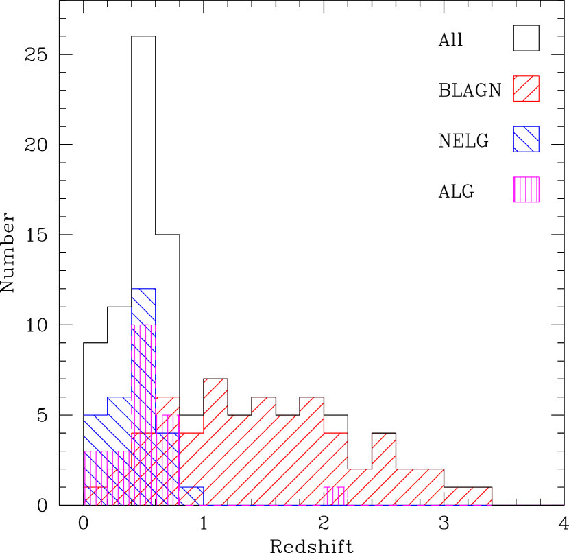
Figure 6.— Redshift histogram of classified extragalactic sources in these 6 fields. Most objects showing no broad line component are below $z=0.8$, likely caused by our typical spectroscopic magnitude limit near 21.

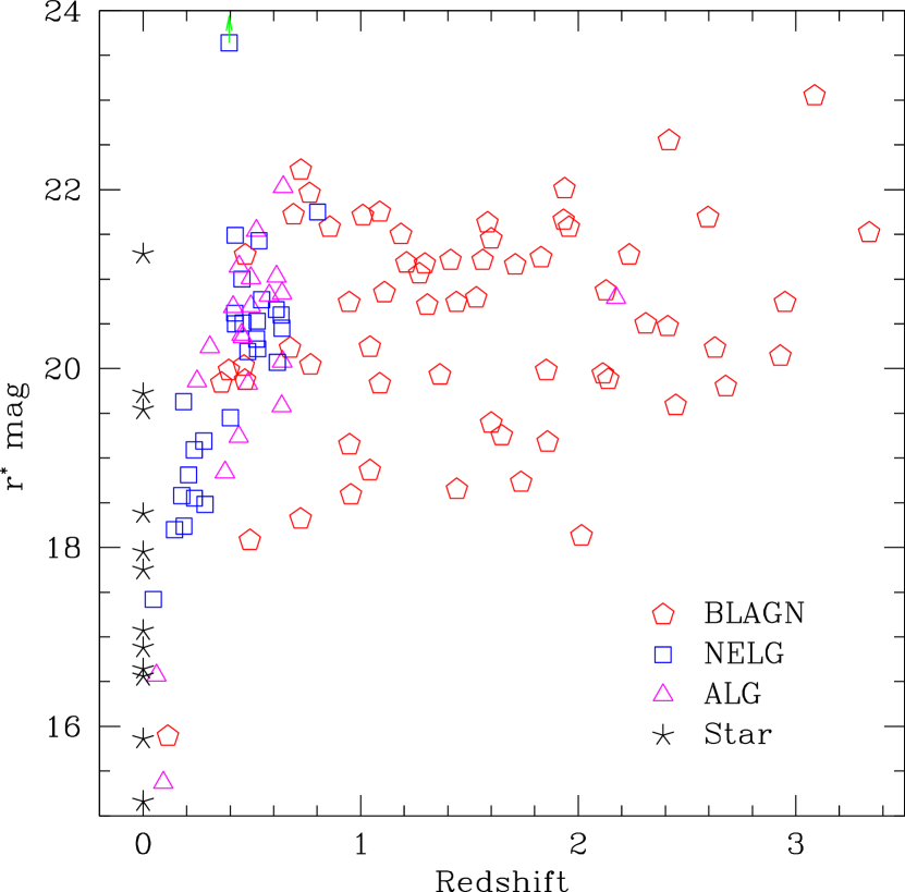
Figure 7.— SDSS $r^{\ast}$  band magnitudes vs. redshift. Galaxies of all types are seen out to $z\sim 0.8$, beyond which they are typically too faint for spectroscopic classification. BLAGN can be detected at all redshifts and extend well beyond our nominal ${r^{\ast}}=21$ spectroscopic limit due to their strong broad emission lines. The wide range of $r^{\ast}$ mags at each redshift reflects both the breadth of object types detected, and the range of exposure time across and between fields.

From galaxies in the Hubble Deep Field with good completeness to $R=23$ (Cohen et al., 2000), the median redshift of galaxies at $R=21$ is about 0.5. By contrast, our median ${r^{\ast}}$ mag for $z=0.5$ galaxies is significantly brighter at that redshift. This may not be due to incompleteness of optical followup; given both the possibility of an AGN contribution and the known correlation between bulge luminosity and black hole mass, we note that X-S galaxies are likely to be atypically luminous in the optical band.

7.2. Luminosities and X-ray/Optical Ratio

Figure 8 shows the 0.5-2 keV X-ray luminosity of spectroscopically classified galaxies and AGN as a function of redshift. BLAGN span a higher range of luminosities than do galaxies, but with some overlap. Overplotted is the sensitivity of the ROSAT Deep Survey assuming their quoted limit $f_{x}=5.5\times 10^{-15}$; (Lehmann et al., 2001). The ChaMP samples luminosities 5–10 times fainter at a given redshift even assuming a more optimistic limit (from their Figure 3) of $2\times 10^{-15}$.

Figure 8.— Wide coverage of the log$~{}L_{X}$  vs. redshift plane highlights the advantages of varying depths and wide sky area of the ChaMP. BLAGN span a higher range of $~{}L_{X}$  than galaxies but with some overlap. The dashed line shows the minimum luminosity corresponding to which the ROSAT Deep Survey was sensitive (see § 7.2).

The slope of a hypothetical power law connecting 2500Å  and 2 keV is defined as ${\alpha_{ox}}\,=0.384~{}{\rm log}\frac{L_{opt}}{L_{X}}$ (where these are monochromatic luminosities at 2500Å  and 2 keV), so that $\alpha_{ox}$  is larger for objects with stronger optical emission relative to X-ray. We note that our definition of $\alpha_{ox}$ here includes no mean $k$-corrections for emission lines, intervening or intrinsic absorbers, so $\alpha_{ox}$ is directly related to ${\rm log}\,\frac{f_{X}}{f_{r}}$ , which we prefer.

O-S AGN samples show typical $\alpha_{ox}$ values of about 1.5 (Green et al., 1995) corresponding to ${\rm log}\,\frac{f_{X}}{f_{r}}=-0.57$. We find for the current sample of ChaMP BLAGN a somewhat lower value of $\overline{{\alpha_{ox}}}=1.36\pm 0.15$ (${\rm log}\,\frac{f_{X}}{f_{r}}=-0.19$). La Franca et al. (1995) found a similar mean $\alpha_{ox}$ of 1.3 for X-S AGN (${\rm log}\,\frac{f_{X}}{f_{r}}=0)$. X-ray surveys select X-ray bright objects by definition, and so are complementary to O-S samples.

A significant correlation between optical luminosity and $\alpha_{ox}$ has been noted in many studies based on O-S quasars (Vignali et al. 2001, 2003; Yuan et al. 1998; Green et al. 1995; Wilkes et al. 1994). One cause might be low-energy X-ray absorption as reported in quasars at higher redshifts (Vignali et al. 2001, Yuan et al. 2000; Fiore et al. 1998; Elvis et al. 1994). Hypothesized to be due to the presence of large gas quantities in primeval galaxies, such absorption might also be related to strong dense gas outflows akin to those seen in broad absorption line (BAL) QSOs. However, the trend in these samples is primarily with $L_{opt}$ and not redshift. Another cause of the apparent trend may be a combination of wider intrinsic population dispersions in $L_{opt}$ than in $L_{X}$ along with superposed selection effects (Yuan et al. 1998, La Franca et al. 1995).

We detect no discernible dependence of $\alpha_{ox}$ on either redshift (Mathur, 2002) or optical luminosity. Figure 9 shows no correlation between ${\rm log}\,\frac{f_{X}}{f_{r}}$  and optical luminosity (which we calculate as $\nu L_{\nu}$ at 2500Å, assuming optical spectral slope $\alpha=-0.5$). Galaxies span a lower but equally wide range of ${\rm log}\,\frac{f_{X}}{f_{r}}$  as do BLAGN. The curve in Figure 9 traces the simulated mean quasar track with $\Delta z=0.5$ redshift bins and imposed limits of ${\rm log}~{}f_{X}=-15$ and ${r^{\ast}}<22$. All input simulated quasars have constant ${\rm log}\,\frac{f_{X}}{f_{r}}=-0.12$ (${\alpha_{ox}}\sim 1.4$). The high luminosity point has $\overline{z}=0.37$, while the faint end has $\overline{z}=4.2.$ No trend is seen in BLAGN for either data or simulation, because the accretion dominates the spectral energy distribution. By contrast, Figure 9 shows a strong correlation between ${\rm log}\,\frac{f_{X}}{f_{r}}$  and X-ray luminosity for galaxies. The trend is likely a combintation of 2 effects, one intrinsic, and one extrinsic: (1) The wide range of ${\rm log}\,\frac{f_{X}}{f_{r}}$  for galaxies may reflect the unlinking of nuclear X-ray luminosity from the optical luminosity, where the latter is strongly affected by host galaxy contributions. (2) The current optical spectroscopic magnitude limit excludes sources that are very weak in optical relative to X-ray emission (have large $\frac{f_{X}}{f_{r}}$) and have small $~{}f_{X}$.

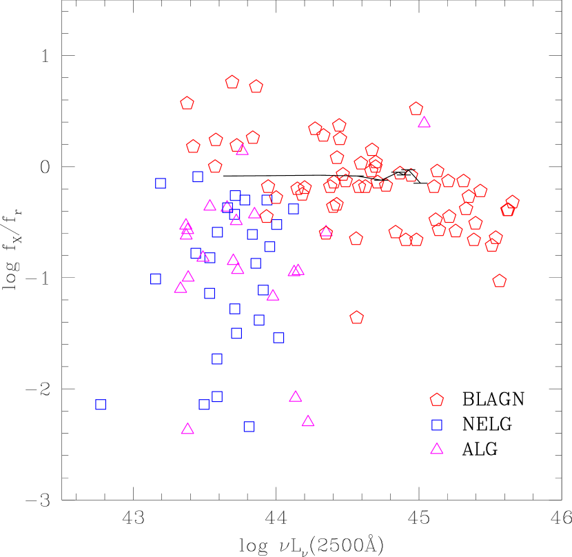
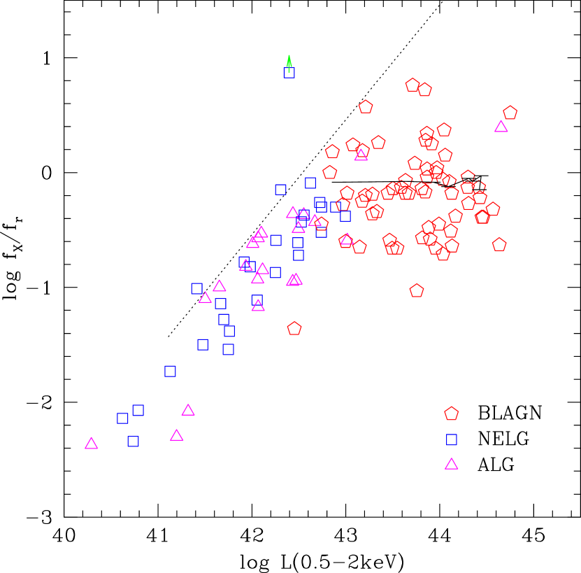
Figure 9.— LEFT: ${\rm log}\,\frac{f_{X}}{f_{r}}$  vs. log$~{}L_{opt}$  shows that galaxies span a range of X-ray to optical flux ratio at least as wide as do BLAGN. The curve traces the mean expected quasar track for $z=0.5$ redshift bins for the simulation described in § 7 and imposed limits of ${\rm log}~{}f_{X}=-15$ and ${r^{\ast}}<22$. All input simulated quasars have constant ${\rm log}\,\frac{f_{X}}{f_{r}}=-0.3$ (corresponding to ${\alpha_{ox}}\sim 1.4$). The high luminosity point has $\overline{z}=0.37$, while the faint end has $\overline{z}=4.2.$ RIGHT: ${\rm log}\,\frac{f_{X}}{f_{r}}$  vs. log$~{}L_{X}$  correlates strongly for galaxies but not BLAGN. The dashed line corresponding to ${r^{\ast}}=22$ and $z=0.5$ is shown for a range of log$~{}f_{X}$  from –16 to –12 to illustrate the effect of our spectroscopic limit. The wide range of ${\rm log}\,\frac{f_{X}}{f_{r}}$  for galaxies may reflect the unlinking of nuclear X-ray luminosity from the optical luminosity, because the latter is strongly affected by host galaxy contributions.

7.3. Colors

The optical colors of ChaMP sources depend on object type, redshift, and reddening. The SDSS provides excellent statistics on the colors of the objects that fall into their spectroscopic sample. The ability to compare the photometric and color properties of X-S sources with SDSS sources is an important ChaMP feature which will be treated in upcoming papers.

Figure 10 shows the optical color distribution of ChaMP sources. The mean stellar locus in these SDSS colors is shown as two light short-dashed lines. The range of BLAGN is similar to O-S quasars, where the expected span of $z<3$ quasars in both $(g^{\ast}-r^{\ast})$ and $(r^{\ast}-i^{\ast})$ is from about –0.5 to 1 (Richards et al., 2001). We plot the curve of the simulated mean quasar track for $z=0.5$ redshift bins for our simulation (with imposed flux limits of ${\rm log}~{}f_{X}=-15$ and ${r^{\ast}}=25$). The first point on the track to leave the stellar locus is at $\overline{z}=3.2$. Without X-ray information, normal quasars are virtually indistinguishable from stars in this color plane until higher redshifts, where quasars redden significantly in $(g^{\ast}-r^{\ast})$, with less change in $(r^{\ast}-i^{\ast})$. The reddest $(g^{\ast}-r^{\ast})$ point on the track corresponds to $\overline{z}=4.6$. Galaxies are generally redder than BLAGN. For ALGs, the 4000Å  break is the strongest color determinant. The mean track of an E/S0 galaxy is shown as a red long-dashed line, using the HyperZ code of Bolzonella, Miralles, & Pelló (2000), assuming a Bruzual-Charlot E/S0 galaxy spectrum and typical E(B-V)$=0.05$ for Galactic dereddening. The $(g^{\ast}-r^{\ast})$ colors of E galaxies redden to ${(g^{\ast}-r^{\ast})}\sim 2$ as the break moves redward from the $g^{\prime}$ to the $r^{\prime}$ band at $z\sim 0.4$, and the track achieves its reddest $(g^{\ast}-r^{\ast})$  at about $z=1$ before looping back blueward to end at $z=1.2$. Several ALGs with $0.4<z<0.6$ are shown with ${(g^{\ast}-r^{\ast})}$ close to 3; with ${\rm log}~{}L_{X}\sim 42$, these are likely to be dust-reddened, low luminosity AGN.

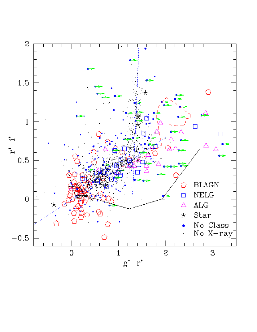
Figure 10.— SDSS $(g^{\ast}-r^{\ast})$  vs. $(r^{\ast}-i^{\ast})$ color-color diagram for objects in 6 ChaMP fields. Optical objects with no X-ray detection are shown as small black points. The typical mean locus of SDSS objects that we use for a sanity check of our photometric calibrations is plotted as 2 short-dashed straight lines. The reddest BLAGN in both colors is at $z=4.93$ (Silverman et al., 2002). The solid curve traces the mean expected quasar track for $z=0.5$ redshift bins for the simulation described in § 7, with imposed flux limits of ${\rm log}~{}f_{X}=-15$ and ${r^{\ast}}=25$. The first point on the track that is away from the stellar locus is at $z=3.2$, while the reddest $(g^{\ast}-r^{\ast})$ point on the track corresponds to $\overline{z}=4.6$. Without X-ray information, normal quasars are virtually indistinguishable from stars in this color plane until $z>3.5$. The mean track of an E/S0 galaxy is shown as a red long-dashed line, using the HyperZ code of Bolzonella, Miralles, & Pelló (2000). The $(g^{\ast}-r^{\ast})$ colors of E galaxies redden to ${(g^{\ast}-r^{\ast})}\sim 2$ as the break moves redward from the $g^{\prime}$ to the $r^{\prime}$ band at $z\sim 0.4$. The loop back blueward in $(g^{\ast}-r^{\ast})$ occurs at $z\sim 1$, where an $L^{*}$ E/S0 has ${r^{\ast}}=23.5$ (Blanton et al., 2001).

The distribution of optical colors changes with X-ray flux as shown in Figure 11. In our spectroscopic sample to date, BLAGN inhabit the full range of X-ray fluxes, but a narrow range of $(g^{\ast}-r^{\ast})$. The brightest X-ray sources are all blue in $(g^{\ast}-r^{\ast})$. The curve in Figure 11 traces the simulated quasar track with imposed flux limits of ${\rm log}~{}f_{X}=-15$ and ${r^{\ast}}=25$. The X-ray bright end point has $\overline{z}=0.37$, while the faint end has $\overline{z}=4.6$ Many of the faint red objects are likely to be high redshift and/or highly absorbed AGN. X-ray faint blue objects may be the wings of the low-redshift quasar $\frac{f_{X}}{f_{r}}$ distribution.

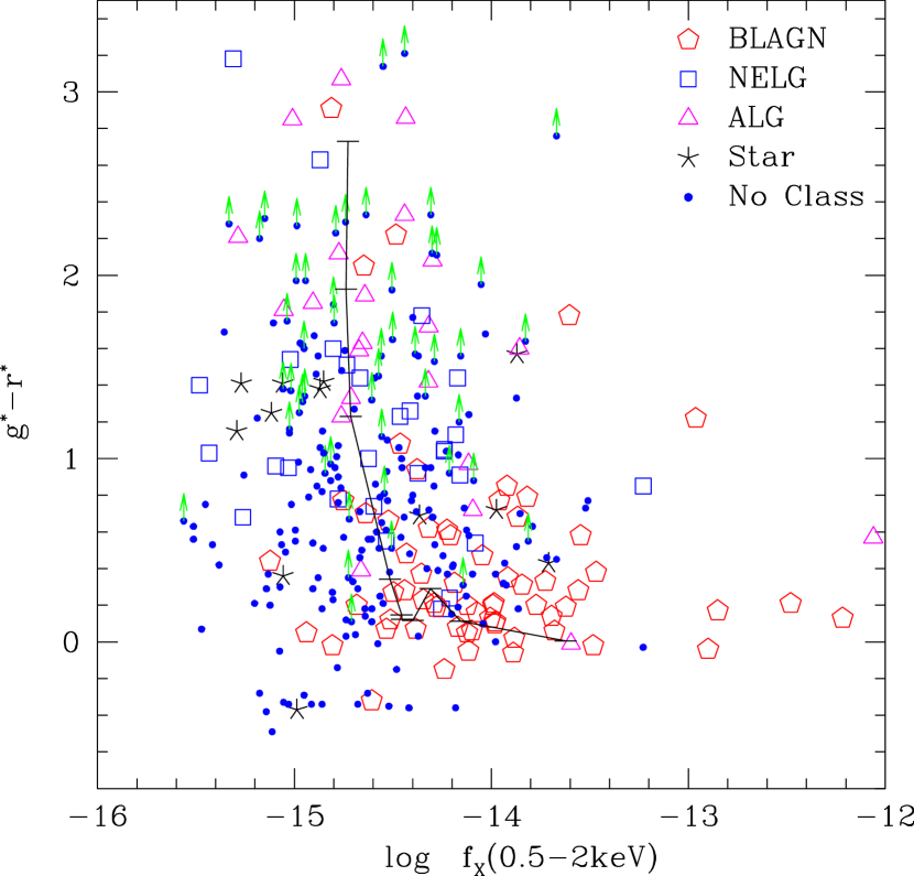
Figure 11.— SDSS $(g^{\prime}-r^{\prime})$  colors derived from our NOAO Mosaic imaging vs. Chandra log$~{}f_{X}$  calculated in the 0.5–2  keV band. Colors include limits (denoted by arrows) when the object is only detected in a single optical filter. The brightest X-ray sources are blue in $(g^{\ast}-r^{\ast})$. The curve traces the mean expected quasar track for $z=0.5$ redshift bins for the simulation described in § 7, with imposed flux limits of ${\rm log}~{}f_{X}=-15$ and ${r^{\ast}}=25$. The bright end point has $\overline{z}=0.37$, while the faint end has $\overline{z}=4.6$

Figure 12 shows SDSS $(g^{\prime}-r^{\prime})$  colors plotted against ${\rm log}\,\frac{f_{X}}{f_{r}}$   in the 0.5–2  keV band. Stars are all at ${\rm log}\,\frac{f_{X}}{f_{r}}<-1$ and ${(g^{\ast}-r^{\ast})}<1.6$. Bright BLAGN cluster strongly at high ${\rm log}\,\frac{f_{X}}{f_{r}}$  and blue $(g^{\prime}-r^{\prime})$ colors. Objects in this part of the plot are largely consistent with O-S quasars and can be classified as such with high confidence even without spectroscopy; a suggested demarcation is shown as the line ${(g^{\ast}-r^{\ast})}<0.3\,{\rm log}\,\frac{f_{X}}{f_{r}}\,+0.7$ in Figure 12. Redder objects with ${\rm log}\,\frac{f_{X}}{f_{r}}>-1$ but ${(g^{\ast}-r^{\ast})}>1$ (many undetected in our $g^{\ast}$-band imaging here) could be one of 2 types. The simulated quasar track shows that some are high redshift ($z>4$) quasars, but many will be obscured AGN, as shown by the high fraction of objects without broad lines in this region.

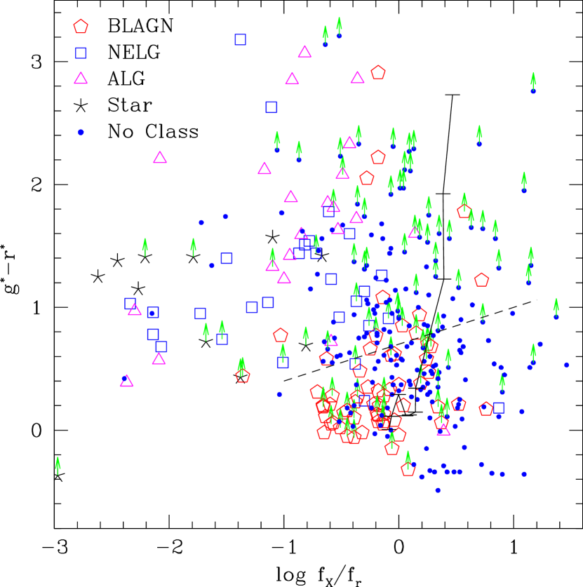
Figure 12.— SDSS $(g^{\prime}-r^{\prime})$  colors derived for Chandra sources from our Mosaic imaging plotted against ${\rm log}\,\frac{f_{X}}{f_{r}}$   in the 0.5–2  keV band. The solid curve traces the mean expected quasar track for $z=0.5$ redshift bins for the simulation described in § 7, with imposed flux limits of ${\rm log}~{}f_{X}=-15$ and ${r^{\ast}}=25$. The bright end point has $\overline{z}=0.37$, while the faint end has $\overline{z}=4.6.$ All input simulated quasars have constant ${\rm log}\,\frac{f_{X}}{f_{r}}=-0.3$, so the shift towards larger ${\rm log}\,\frac{f_{X}}{f_{r}}$  arises only from the imposed flux limits. Objects in the lower right part of the plot are largely consistent with O-S quasars and can be classified as such with high confidence even without spectroscopy; a possible demarcation is shown as the dotted line ${(g^{\ast}-r^{\ast})}<0.3\,{\rm log}\,\frac{f_{X}}{f_{r}}\,+0.7$. Clustered with stars at low ${\rm log}\,\frac{f_{X}}{f_{r}}$   are galaxies that likely have little X-ray contribution from an active nucleus.

7.4. X-ray Bright Galaxies with no Emission Lines

A small number of X-ray bright, optical normal galaxies (Comastri et al., 2002) have also been found in XMM and Chandra  surveys. These objects show at best weak optical emission lines. We propose three possible explanations for X-ray luminous objects showing no broad optical emission lines. (1) A ’buried AGN’ - a nucleus that is intrinsically similar to that of a quasar but whose optical continuum and broad emission line region are shrouded by a large obscuring column. (2) A low luminosity AGN (LLAGN) where the host galaxy light dominates light in the spectral aperture. One such type of LLAGN may host a nucleus with a massive black hole accreting at very low rates, i.e., an advection dominated accretion flow (ADAF). (3) A BL Lac object.

7.4.1 Buried AGN

The unified model explains the Seyfert classes 1 & 2 as different views of the same phenomenon (Antonucci, 1993). Quasars are thought to be luminous versions of Seyfert galaxies, so this unified (orientation + obscuration) scheme should hold for quasars, i.e., they should have a similar nucleus and dusty torus system in their center. Seyfert 2 galaxies outnumber Seyfert 1 galaxies 4:1 in the local universe, which is consistent with the covering factor of the obscuring tori (Maiolino & Rieke, 1995), and if that ratio can be extrapolated to higher luminosities, then we should expect many Type 2 quasars to be detectable in the high-redshift universe. Only a few Type 2 quasars have been convincingly detected to date (Akiyama et al. 2002, Norman et al. 2002, Stern et al. 2001, Schmidt et al. 2002), implying a strong, perhaps luminosity-dependent evolution (Franceschini, Braito, & Fadda, 2002). However, infrared surveys are currently finding bona fide Type 2 quasars. Several of the IRAS Hyperluminous Galaxies (Beichman et al. 1986; Low et al. 1988, 1989) have been shown to be Type 2 quasars (e.g., Wills et al. 1992; Hines & Wills 1995; Hines et al. 1995). More recently, samples selected from the 2MASS include a large number of Type 2 objects with quasar-like near-IR luminosities. Fully 1/3 of the spectroscopically confirmed AGN in the 2MASS are Type 2 objects (Cutri, 2001). Extrapolating to the entire sky, 2MASS should detect roughly 5,000 such objects with $K<15$, many of which will have IR luminosities in the quasar range (Smith et al., 2002). Near-IR surveys are less biased against absorption and less sensitive to orientation than optical surveys, but will preferentially select samples with high star formation rates and copious dust.

The X-ray characteristics of 2MASS quasars suggest strong absorption (${\rm N_{H}}\sim 10^{22}{\rm~{}cm^{-2}}$; Wilkes et al. 2002) with contributions from direct and unabsorbed, scattered, and/or extended emission. The possibility remains that they are intrinsically X-ray-weak. The sample of 2MASS quasars studied with Chandra by Wilkes et al. (2002) are all at $z<0.3$ (due to the 2MASS $K\sim 14.5$ limit). At higher redshifts, the reduced effective column in the X-ray bandpass should be effective in discovering Type 2 quasars, and help resolve the question of their intrinsic X-ray luminosities. How can and should a Type 2 quasar be recognized in an X-ray survey? Not simply on the basis of X-ray hardness. High column density X-ray-absorbing gas (e.g., a warm absorber) may be interior to the putative obscuring torus, so that even normal optical Type 1 (broad line) quasars may show low luminosity and/or high column absorption in the X-rays (however in these cases absorption in the restframe UV is usually apparent; Green et al. 2001; Brandt, Laor, & Wills 2000). Luminosity criteria may be subtle, since the claim for high-$L$ could be based on either $L_{opt}$ or $L_{X}$, perhaps including large absorption-corrections. We find objects in our sample that show signs of X-ray or optical absorption, or both, but with no strong evidence that these properties are coupled.

If an X-S AGN is found showing no broad emission lines, oftentimes the search for broad lines may be very limited, including only what is seen on a discovery optical spectrum. A search for broad H$\alpha$ is sometimes possible from the ground, and may reveal instead a luminous Type 1.9 quasar (Akiyama, Ueda, & Ohta, 2002), but the classification is by nature somewhat arbitrary. Spectropolarimetry can reveal broad line flux, but since those same photons must also be in the total flux spectrum, broad line detection becomes a question of adequate $\frac{S}{N}$. Indeed, many IR-selected Type 2 quasars show lower fractional polarization than Type 1 quasars, presumably because of strong stellar light contributions (Smith et al., 2002). Furthermore, there are few objects for which we can convincingly claim an optical Type 2 classification without examining line ratios in detail in spectra of higher $\frac{S}{N}$. Instead we define a “buried AGN” here as an object that has either no or only narrow emission lines in optical spectra, strong evidence for log${\rm N_{H}}>22$ in the rest-frame, and ${\rm log}~{}L_{X}>43$ without absorption-correction. If the signature of X-ray absorption is clearly detected, then an absorption-corrected ${\rm log}~{}L_{X}>44$ qualifies as a Type 2 quasar candidate, with confirmation pending high ${\frac{S}{N}}$ followup spectroscopy. We find no such objects in these 6 fields.

7.4.2 Low-Luminosity AGN

Many of these X-ray selected galaxies are so distant that their angular diameters are comparable to the slit (or fiber) widths used in ground-based spectroscopic observations. Using integrated spectra of a sample of nearby, well-studied Seyfert 2 galaxies, Moran, Filippenko, & Chornock (2002) demonstrate that the defining spectral signatures of Seyfert 2s can be hidden by light from their host galaxies. At $z\sim 0.6$, a 1.5″  slit encompasses a region about 10 kpc, which includes a substantial fraction of the host starlight emission. Some 60% of the observed objects would not be classified as Seyfert 2s on the basis of their integrated spectra, which is comparable to the fraction of Chandra  sources identified as “normal galaxies” in deep surveys (Hornschemeier et al. 2001; Barger et al. 2002).

These ’buried AGN’ may host low rate (advection dominated) accretion flows (ADAFs; Narayan & Yi 1995). The X-ray spectra produced by ADAFs are relatively hard, so ADAF sources may contribute a fair share of the hard ($>$2 keV) background (Yi & Boughn, 1998). Half of the 2-10 keV CXRB could consist of low-luminosity ($L_{X}<10^{41}$ ergs/s) sources if the comoving number density is $\sim 3\times 10^{-3}$ Mpc^-3, comparable to the density of $L^{*}$ galaxies (e.g., Peebles 1993). ADAF sources should be characterized by inverted radio spectra $I_{\nu}\propto\nu^{0.4}$

There are 8 optical counterparts to X-ray sources in the current sample that have hard band luminosities log$L$(2–8 keV) $>43$ and no signs of broad optical emission lines in their spectra. The luminosity in this band is plotted against hardness ratio in the right panel of Figure 13. (A similar $L_{X}$ criterion in the 0.5–2 keV band would be log$L$(0.5-2 keV) $>42.4$) Half of these Type 2 candidates are hard, with $HR_{0}>0$. Optical spectra of this sample are shown in Figure 14. Several of these objects have spectra of absorption line galaxies with only a weak narrow [OII] emission line. Several counterparts are also classified as narrow emission line galaxies with strong lines of [OII], [OIII] and H$\beta$. All these objects are at redshifts less than unity.

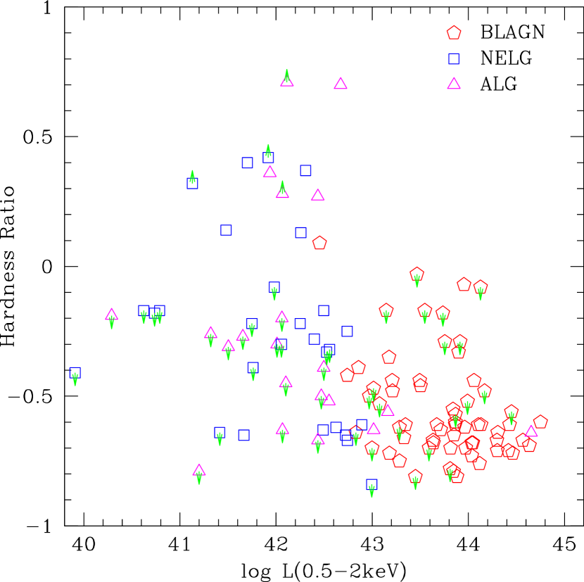
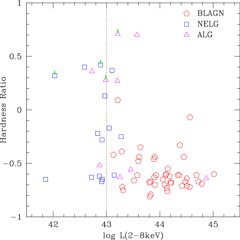
Figure 13.— Hardness ratio vs. X-ray luminosity in 2 bands. Most of the luminous objects (quasars) are soft. This may arise both because they are at high redshift (where absorption causes smaller changes in hardness) and because they are intrinsically less obscured. RIGHT: Plotting against a harder $L_{X}$(2-8 keV) does not significantly change the plot. A dashed line shows our criterion for objects with no broad lines to be classified as ’buried AGN’; log$L_{X}$(2-8  keV)$=43$.

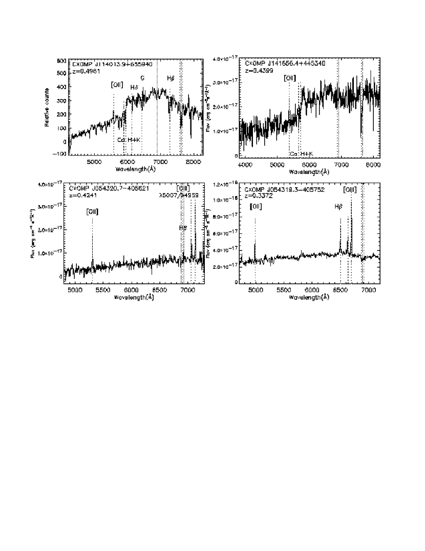
Figure 14.— Spectra of ChaMP candidate absorbed AGN. These optical spectra correspond to 4 X-ray sources with luminosities (log$L_{X}$(2-8 keV)$>43$ erg s^-1), hard X-ray spectra, and no signs of broad emission lines characteristic of optically-selected quasars. Grey regions mark the telluric absorption bands.

Newer CXRB models attempt to include the observation that most hard faint sources from Chandra and XMM Newton surveys are objects at $z<1$, which requires a very different evolution rate for Type 1 and Type 2 objects. This must at least modify the meaning of Unification; all Type 2 AGN are not necessarily Type 1 from a different angle. The covering fraction of the putative obscuring torus may also change, and probably evolves statistically with cosmic time. The relative dearth of high redshift Type 2 quasars could be explained by selection effects. As discussed in § 7.1, these objects may simply fall below our optical detection limits, or at least our ${r^{\ast}}=22$ spectroscopic limit. Since these objects have low surface densities, as the ChaMP area grows, a volume-limited subsample will help define their relative space densities.

7.4.3 BL Lacs?

The first known BL Lacs provided the three observational characteristics of the class (e.g., Stein, Odell, & Strittmatter 1976; Angel & Stockman 1980), repeated here as presented by Jannuzi, Smith & Elston (1993): ”1.) They are intrinsically luminous with strong and ‘rapid’ variability. (BL Lac objects have been observed to vary at X-ray, optical, infrared, and radio wavelengths.) 2.) They have ‘featureless’ optical spectra. (How to define ”featureless” has been a question for debate […]). 3.) The electro-magnetic radiation from BL Lac objects is observed to be linearly polarized.” In general the polarization requirement has been for the observed degree of polarization to be larger than that possible from differential extinction (at most wavelengths a percentage polarization of greater than 3%) or for the degree and/or position angle of the polarization to be variable. Together, these observationally based criteria reflect what we now know is the distinguishing physical characteristic of all BL Lacs, the presence of a strong source of synchrotron radiation in these sources.

We are interested in the identification of BL Lacs because it is possible that with only single epoch photometry and spectroscopy (and no polarimetry data), objects which we have currently identified as buried AGN might be BL Lac objects. Lacking strong emission lines, the optical and near-IR spectra of many BL Lacs (particularly X-ray selected objects; see EMSS survey results of Morris et al. 1991 and Jannuzi, Elston & Smith 1994) can be dominated by host galaxy starlight and look very similar to what we call absorption line galaxies.

While more data on these objects would be advantageous, we have checked whether BL Lacs might be hidden in our absorption line galaxy sample. First, we checked for known radio emission from our X-ray sample. Since all known BL Lac objects are strong radio sources (e.g. Jannuzi 1990; Stocke et al. 1990), the presence of strong emission (from a compact synchrotron core) might indicate the presence of a BL Lac. Unfortunately, no data are available of sufficient sensitivity for our ALGs. Our cross-correlation of our X-ray source list to the FIRST (White et al., 1997) and NVSS (Condon et al., 1998) radio surveys with a 5″  search radius did yield 2 matches to other sources. One is a bright nearby radio-quiet Sy 1 and the other is likely to be a distant radio-loud quasar (see Appendix A). Second, we checked the strength of the 4000Å  break in our spectra of all sources we classed as ALGs or BL Lacs (all those with the strongest emission line equivalent width $W_{\lambda}<5$Å). As discussed by the EMSS team, a weak break might indicate the presence of non-thermal (featureless) emission contributing to the total emission – again a possible sign of a BL Lac being present in the source. We measured the 4000Å  break contrast using the using the definition of Dressler & Shechtman (1987)

$${\rm Br}_{4000\AA}=\frac{f^{+}-f^{-}}{f^{+}}$$

where $f^{+}$ is the average flux in the rest wavelength range 4050–4250Å and $f^{-}$ the average flux between 3750–3950Å. As long as the $\frac{S}{N}$ in this wavelength region exceeds 5 per pixel, we count break strengths $<0.25$ as BL Lac candidates pending confirmation from any of the 3 criteria listed above.

We found just one optical spectroscopic BL Lac candidate; CXOMP J05421.5-410206, with ${r^{\ast}}=19.6$ at $z=0.637$. While in the same range of luminosity as known BL Lac objects, it has a relatively low ${\rm log}\,\frac{f_{X}}{f_{r}}=-0.6$. We note that for optical magnitudes $V<20$, the optical luminosity function for X-ray-selected BL Lacs yields a surface density of about 160 steradian^-1 or about 0.05 deg^-2 (Wolter et al., 1994). The optical QSO surface density is about 600 times as high at similar magnitudes (Meyer et al., 2001), so few BL Lacs are expected overall in the ChaMP.

7.5. Signs of Absorption?

Figure 15 shows $HR$ values corrected as described in § 3. Many previous studies have assumed that when total source counts exceed 30 or 50, that the $HR$ values are reliable without accounting for errors. In fact, the combination of source spectrum and telescope effective area may require a surprisingly large number of counts just to achieve detection in all the bands composing an $HR$ calculation. The fraction of limits (mostly upper limits, since Chandra’s $H$ band sensitivity is significantly lower) decreases below 10% only above about 120 counts (for these observations typically at about ${\rm log}~{}f_{X}=-14$ in Figure 15). About half the sources have $HR_{0}$ upper limits even for sources with 30 counts or more. Analysis of only those points detected in both bands would lead to an apparent hardening at low fluxes. Correctly incorporating the upper limits via survival analysis (ASURV Rev 1.1 Isobe & Feigelson 1990; LaValley, Isobe & Feigelson 1992), we find no significant evidence for hardening of the spectra toward lower fluxes. Excluding sources with fewer than 30 (0.3-8 keV) counts, the median (mean) of $HR_{0}$ for sources with $<120$ counts is –0.66 ($-0.58\pm 0.02$), while for sources with more counts we find –0.62 ($-0.56\pm 0.03$). This is not inconsistent with the conclusion in Kim et al. (2003b) that spectral hardening at faint fluxes is significant only in the softest band (S1; 0.3-0.9 keV) and thus most likely due to absorption. While spectral hardening towards fainter fluxes may be real, careful accounting for errors in hardness ratios is important: spectral stacking (e.g., Brandt et al. 2001; Tozzi et al. 2001) is a powerful alternative for these analyses.

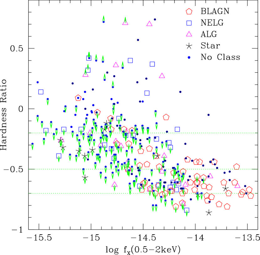
Figure 15.— Corrected hardness ratios $HR=(H-S)/(H+S)$ as a function of X-ray flux. $HR$ values here are corrected to represent a source on-axis on a front-illuminated (FI) chip, and to include upper or lower limits to $HR_{0}$ (arrows), based on $2\sigma$ upper limits to $H$ or $S$ counts, respectively. Horizontal dashed lines show the $HR_{0}$ corresponding to a typical unabsorbed AGN (bottom; $\Gamma=1.9/{\rm N_{H}}=0$ cm^-2), the average hardness ratio of the total CXRB spectrum (middle; $\Gamma=1.4/{\rm N_{H}}=0$ or $\Gamma=1.9/{\rm log\,N_{H}}\geq 21.5$), and a highly absorbed AGN (top; $\Gamma=1.9/{\rm log\,N_{H}}\geq 22$). Most BLAGN likely suffer some moderate absorption, whereas a large fraction of NELG and ALG show evidence for ${\rm log\,N_{H}}\geq 22$. The brightest 8 sources between $-13.4<{\rm log}~{}f_{X}<-12$ (typically soft) are left outside the plot range for clarity.

Assuming that $\Gamma\sim 1.9$ for most BLAGN, the hardness ratios indicate that most BLAGN likely suffer some absorption, whereas strong absorption is rare. A much larger fraction of NELG and ALG show evidence for ${\rm log\,N_{H}}\geq 22$.

X-S quasar samples may be less biased against absorbers (both intrinsic and line-of-sight) than are O-S samples. This advantage is expected to be especially important at high redshifts for two reasons. First, X-rays from high-$z$ objects can be detected through a larger intrinsic absorbing column of gas and dust because the observed-frame X-ray bandpass corresponds to higher energy, more penetrating X-rays at the source; the observed-frame, effective absorbing column is $N_{\rm H}^{\rm eff}\sim N_{\rm H}/(1+z)^{2.6}$ (Wilman & Fabian, 1999). Second, optical color criteria for high-$z$ candidates (e.g., blue filter dropouts) tend to select objects with strong Ly$\alpha$ forest decrements.

Do red optical colors reliably predict hard X-ray spectra or vice-versa? Figure 16 shows two quantities, $HR_{0}$ and $(g^{\ast}-r^{\ast})$, which may serve as crude proxies for absorption measurements. While $(g^{\ast}-r^{\ast})$ is affected by dust via optical reddening, it is also strongly dependent on object type, host galaxy fraction, and redshift. While the hardness ratio $HR_{0}$ is affected by the total X-ray absorbing column, it is also dependent on redshift since the effective column decreases as noted above. We find no overall correlation between these two absorption indicators, as is evident from Figure 16. X-ray and optical absorption are effectively decoupled for several physical reasons: 1) The gas-to-dust ratio varies, depending on densities, abundances, and ionization level (Maiolino et al., 2001). 2) Physically distinct absorbing regions (Weingartner & Murray, 2002). 3) Variations in geometry, reflection, and self-shielding (Elvis, 2000).

We note that for the 35 X-ray hard objects ($HR_{0}>0$) suggestive of strong absorption, there is some weak evidence for a trend in Figure 16. Using ASURV (LaValley, Isobe & Feigelson, 1992), we include the limits in both axes, and find no significant correlation (probability of no correlation is $9.8\%$). At high columns, other scatter-inducing factors such as redshift, orientation, and/or reflection may be overcome by the effects of intrinsic dusty absorbers. This suggests that the correlation should be tested with a larger sample, as will become rapidly available from the ChaMP.

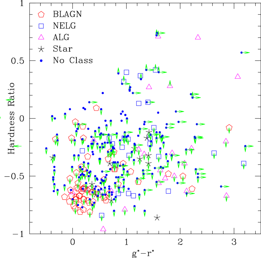
Figure 16.— SDSS $(g^{\prime}-r^{\prime})$  colors derived from our 4m Mosaic imaging vs. corrected Chandra hardness ratio $HR_{0}$. Since a range of redshifts and optical object types may pertain, $(g^{\ast}-r^{\ast})$ is at best a crude measure of optical reddening - as is $HR_{0}$ for X-ray absorbing column. Nevertheless, above $HR_{0}\sim 0$ a weak correlation exists between these indicators ($P=10\%$; see § 7.5). This suggests that at high columns, the effects of intrinsic dusty absorbers may dominate the dispersion induced by factors such as redshift, orientation, and/or reflection.

Hard red objects in the upper right hand corner of the plot (e.g., $HR_{0}>0$ and ${(g^{\ast}-r^{\ast})}>1.5$) likely contain a high fraction of obscured AGN; none with spectral classifications to date are BLAGN. Soft red objects in the lower right (e.g., $HR_{0}<0$ and ${(g^{\ast}-r^{\ast})}>1.5$) could be high redshift AGN (where unabsorbed X-rays are shifted into the Chandra passband) or soft galaxies above $z\sim 0.3$. Spectra of the hard blue BLAGN (e.g., $HR_{0}>-0.2$ and ${(g^{\ast}-r^{\ast})}<0.5$) show mostly weak narrow emission lines, and several appear to have significant blueshifted CIV absorption. These objects are similar to BALQSOs, which are only slightly reddened (Reichard et al., 2003) but known to be heavily absorbed in X-rays (Green et al., 2001).

7.6. Clusters of Galaxies

Clusters are important probes of cosmology, especially at high mass and redshift. In general, a surface density of $>0.003\,$deg^-2 for clusters more massive than Coma above $z>1$ violates $\Lambda$CDM cosmologies at 95% confidence (Evrard et al., 2002). Evolution of and correlations between X-ray temperature, luminosity, and gas mass in clusters (Vikhlinin et al., 2000) enables the strongest available constraints on hierarchical models. Chandra’s high sensitivity, low background and good spatial resolution facilitate the detection of spatially extended emission which at high galactic latitudes corresponds to emission from groups or clusters of galaxies.

Our prototype X-ray extended source detection algorithm works by performing photometry in annuli around sources detected by wavdetect, and compares the best-fit gaussian and beta models to the expected PSF size. All of the targeted clusters are detected. Some clusters also have point-like emission from a cD galaxy or quasar, which can confuse the automated algorithm. These are generally noticed during our visual inspection, which also provides an opportunity to flag any X-ray source surrounded by a concentration of optical galaxies. Using this approach, we have found 3 serendipitous clusters in these 6 fields, each of which described further below. The ChaMP makes feasible simultaneous optical and X-ray searches for clusters. Further refinement and testing of cluster selection is underway (Perley et al., 2004) that combines automated and by-eye X-ray source extent determinations, Voronoi Tesselation and Percolation analysis on color-filtered optical images, and red sequence identification in optical color-magnitude plots.

7.6.1 CXOMP J033912.2-352614

During our standard visual inspection of each X-ray source, we noted extended X-ray emission centered near $03^{h}39^{m}12.2^{s}\,-35^{\circ}26\arcmin\ 15.0\arcsec$. Figure 17 shows the X-ray and optical $r^{\prime}$ band image of the region. A $\beta$ model to fit the cluster profile is unconstrained, but fixing to an average cluster value of $\beta=0.6$ (Jones & Forman, 1984), we derive a core-radius $r_{c}=47\pm 12\arcsec$ and 2821 counts (0.7-2 keV). The (0.5-2 keV) flux is therefore $3\times 10^{-13}$ erg cm^-2 s^-1. This estimate may be affected (at the $\sim 20\%$ level) by emission from the extended halo of the central bright (10th mag) galaxy of the Fornax cluster, NGC 1399, which lies $9\arcmin$ to the west outside the Chandra field of view (Paolillo et al. 2002).

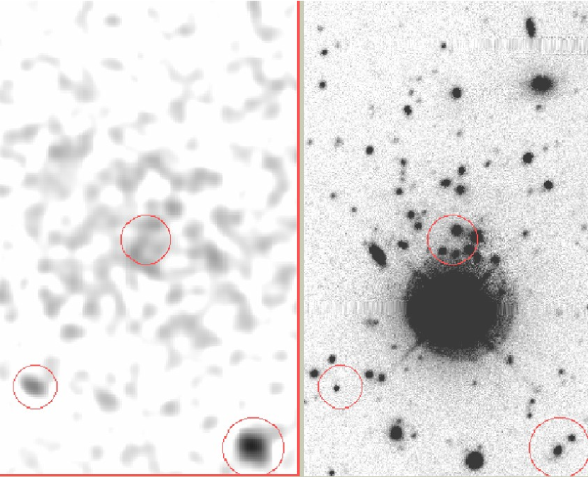
Figure 17.— CXOMP J033912.2-352614. LEFT: We note extended X-ray emission centered near $\alpha=03~{}39~{}12.2,~{}\delta=-35~{}26~{}15$ in this ACIS-S image from ObsID 624. The field is approximately 2′ NS, and 1.3′ EW. The orientation (in this and all images herein) is N up and E to the left. Circles show the positions of detected X-ray sources, with circle size corresponding to the Chandra 95% EE at this off-axis angle. RIGHT: Our CTIO4m/Mosaic imaging indeed shows a cluster of galaxies just N of a $V=12$ star. The bright star is not the X-ray source since it is 19.5″ South of the X-ray centroid, and stars do not generally produce diffuse X-ray emission.

In our optical imaging, the source corresponds to what appears to be a cluster of galaxies just N of a bright ($V=12$ mag) star. Figure 17 shows the optical $r^{\prime}$ band image of the cluster next to the (2-pixel gaussian) smoothed X-ray image. We are confident that the X-ray emission does not originate from the star. Stars do not produce significantly extended X-ray emission. Even if they did, the star could not reasonably be associated with the diffuse emission situated as it is at 1.7 core radii (20″) from the emission centroid. As explored by Perley et al. (2004), the $(g^{\ast}-r^{\ast})\sim 2.5$ colors of galaxies within 18″  of the X-ray centroid define a red sequence corresponding to cluster elliptical galaxies at $z\sim 0.4-0.5.$

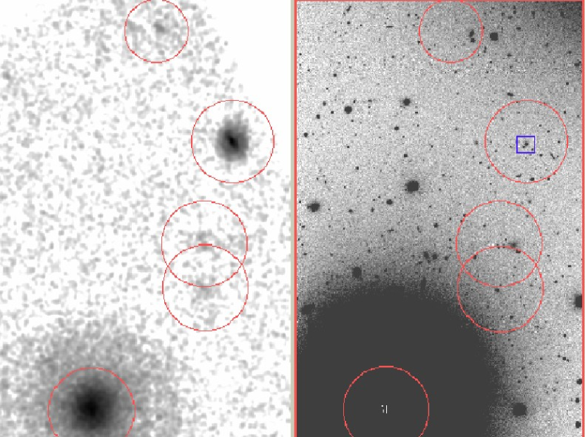
Figure 18.— CXOMP J033841.4-353133. Smoothed ACIS-I (LEFT) and optical $r^{\prime}$ image (RIGHT) of the field in ObsID 624 containing a bright background quasar (see § A.3). Each image is oriented N up, E to the left, covering 6.7′N-S and 4.3′E-W. The BLAGN at $z=0.3597$ is marked by a box in the optical image. Circles represent the Chandra 95% EE radius. The large (37″) EE radius and apparent non-point morphology of the X-ray source reflect the PSF at this large (12.6′) off-axis angle.

7.6.2 CXOMP J054240.9-405515

The bright EXOSAT and ROSAT All-Sky Survey X-ray source EXO 0541.0-4056 was studied in the ASCA Medium Sensitivity Survey as 1AXG J054242-4054. Our spectrum reveals a BLAGN at $z=0.7243$, but the X-ray image clearly shows extended emission out to $\geq 40\arcsec$ from the quasar (Figure 19). A different stretch and zoom of the same region is shown at the top of Figure 4. To better examine the cluster emission, we first created an image in the 0.7-2 keV band only, and masked out all point sources and the quasar with a circle of 4.5″radius. After smoothing the masked image with a 6″ Gaussian, we determined the peak of the diffuse emission to be at $05^{h}42^{m}40.4^{s}\,-40^{\circ}55\arcmin\ 7.0\arcsec$, the NE of the quasar, corresponding to a projected distance of $\sim 80$kpc, assuming the quasar and cluster are at the same redshift. Since the cluster emission centroid is offset by nearly $r_{c}$ from the brightest cluster galaxy (the quasar), this cluster is not relaxed, and is most likely still sloshing from a merger. The fraction of such offsets as a function of redshift is potentially a powerful probe of cluster evolution (Cohn, Bagla, & White, 2001).

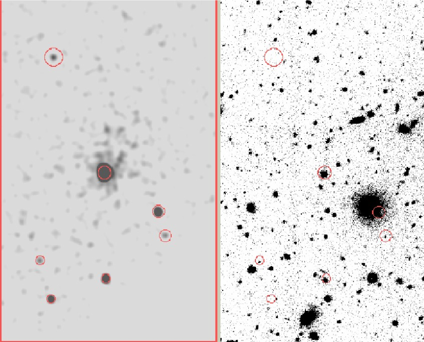
Figure 19.— CXOMP J054240.9-405515. This source has well over 5000 counts in this ACIS-I image (LEFT), and shows a sharp peak with significant ($\sim 40\arcsec$) extent (see also the top panel of Figure 4 for a close-up). Our optical spectrum of the corresponding ${r^{\ast}}=18.3$ object (RIGHT) centered in each of these images (230″ N-S, 140″ E-W) reveals a $z=0.724$ BLAGN (see § 7.6.2). The extended emission quite likely arises in a cluster of galaxies whose members are several mag fainter than the quasar.

Extracting a profile around the cluster centroid, we find the cluster is well-fit with a $\beta$-model of core radius $r_{c}=12\pm 2.5\arcsec$, with $\beta=0.6\pm 0.07$ and total flux of $340\pm 40$ counts, fitting down to the background intensity of 0.03 counts/pixel. The corresponding cluster flux of $3.6\times 10^{-14}$ erg cm^-2 s^-1corresponds to a cluster luminosity of $10^{44}$erg s^-1.

Deep imaging at fine spatial resolution also reveals evidence in the optical and near-infrared for clusters of galaxies around (radio loud) quasars (Yee & Ellingson, 1993) at similar redshifts (Sanchez & Gonzalez-Serrano, 2002). These quasars often do not inhabit the cluster cores, which may support the interaction/merger hypotheses for their fueling, since lower velocities at large radii enhance merging efficiency (Bekki & Noguchi, 1994).

7.6.3 CXOMP J234815.7+005350

The X-ray emission from this object is consistent with a point source, but the optical image looks convincingly like an intermediate redshift group or cluster of galaxies (Figure 20). We tentatively assign a redshift of $z=0.41$ to the cluster, based on a spectrum (Magellan 6.5m with LDSS2 03 Dec 2002) of the brightest ${r^{\ast}}=19.7$ galaxy. The source flux of $f_{X}=1.0\times 10^{-15}$ erg cm^-2 s^-1  at this redshift corresponds to ${\rm log}~{}L_{X}=41.84$. If there is no significant contribution from cluster emission, the evidence suggests that an X-ray bright elliptical galaxy dominates the group. The object is not likely to be a BL Lac because the CaII break strength is normal for an elliptical galaxy ($0.57\pm 0.1$). Some diffuse optical emission may be from the bright extended disk of the host galaxy ($\sim 15$ kpc in radius), in which case a knot of optical emission near the X-ray centroid suggests the possibility of an ultraluminous X-ray source (ULX) in the host. However, this would be 30 times brighter than the brightest known ULX in the Antenna galaxies (Zezas & Fabbiano, 2002) or M82 (Kaaret et al., 2001). Also, we would expect to see strong optical emission lines from the associate star formation regions in the disk.

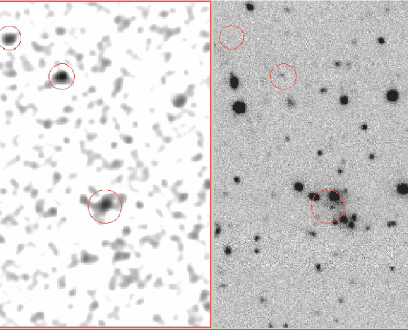
Figure 20.— CXOMP J234815.7+005350. LEFT: The X-ray source has just $31\pm 8$ counts in this ACIS-S image and morphology consistent with a point source. Circles show the 95% EE PSF size, which has radius 6″ at this off-axis angle (4.8′). RIGHT: The $r^{\prime}$ band image shows a group of galaxies coincident near the X-ray centroid. From our optical spectrum (Magellan 6.5m with LDSS2 03 Dec 2002), we tentatively identify the brightest ${r^{\ast}}=19.7$ galaxy just NW of the X-ray centroid as a $z=0.4$ absorption line galaxy (see § 7.6.3). Both images are 240″ N-S, 90″ E-W in size.

8. Multiple Sources

Close X-ray sources ($<10\arcsec$) with optical counterparts are good lens candidates, especially if there is also extended emission signifying a massive potential. They are also interesting for study of the effects of interactions/mergers on activity (Green et al., 2002). Sources with larger separations where one lacks an optical counterpart are good candidates for X-ray jets, whose emission barely dims at all with distance (Schwartz, 2002). We have so far identified 2 close pairs of X-ray sources in these 6 fields.

We find a new close pair of X-ray sources with optical counterparts in the field of ObsID 861, as shown in Figure 21. A Magellan spectrum from 14 July 2002 reveals that the brighter object CXOMP J234835.3+005832 is a $z=0.95$ BLAGN. Since the 90% encircled energy (EE) PSFs of these sources overlap, we estimated their individual counts as follows. We first measure the counts for each source in a core radius of 3pixels. We then measure the total counts in the union of 2 aperture of radius of 10.4 pixels (5″) encompassing both sources, and apportion the total counts to each according their core counts ratio. The fainter source CXOMP J234835.5+015836 is beyond our spectroscopic survey limit, but should be followed up as a lens candidate. The 2 objects’ $\frac{f_{X}}{f_{r}}$ values differ significantly, (with ${\rm log}\,\frac{f_{X}}{f_{r}}=0.72$ and 0.34 for the fainter and brighter object, respectively) so we believe that they are unlikely to be lensed. However, not all lensed objects are achromatic across a wide range in frequency; microlensing, time variability and differential absorption are possible reasons (e.g., Green et al. 2002; Morgan et al. 2001).

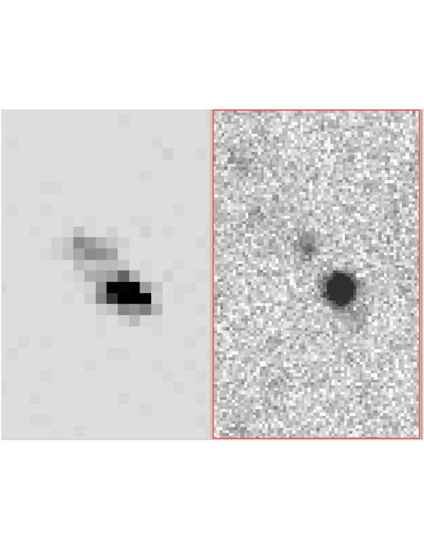
Figure 21.— The pair of X-ray sources shown here - CXMOP J234835.3+005832 and CXOMP J234835.5+005836 - are separated by 4.9″ in the ACIS-S image (LEFT), and both have reliable optical counterparts in our Mosaic $r^{\prime}$band image (RIGHT). The field shown is approximately 30″ NS, and 18″ EW. Our spectrum of the brighter more southern object shows it to be a BLAGN at $z=0.9469$. Spectroscopic follow-up of the fainter object ${i^{\ast}}=23.3$ should help determine whether the system is lensed.

CXOMP J234758.0+010329 is an ${r^{\ast}}=20.1$ ALG at $z=0.2481$. As shown in Figure 22, CXOMP J234758.9+010343 and CXOMP J234758.0+010329 are separated by only 10″, and both appear to belong to a group of galaxies. We detected no extended emission from the group.

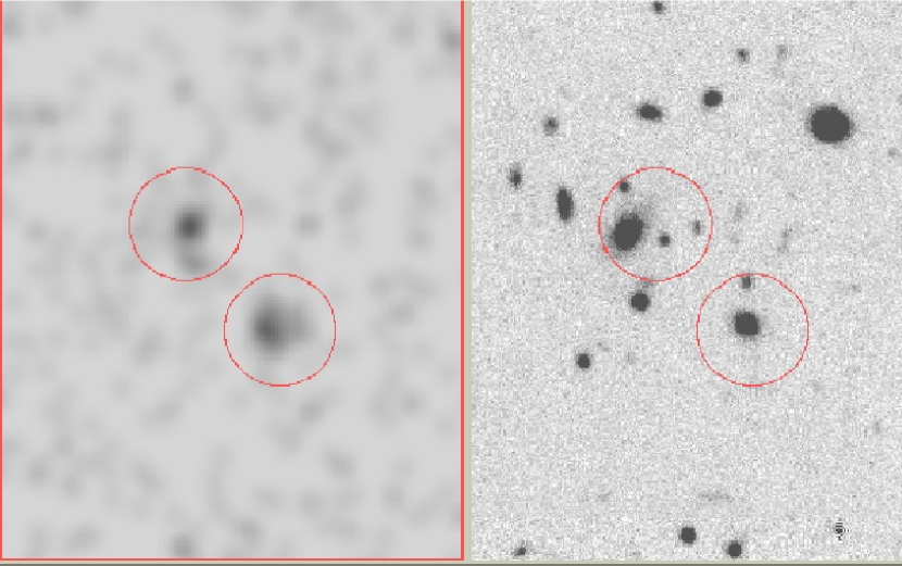
Figure 22.— X-ray (LEFT) and optical $r^{\prime}$-band (RIGHT) images of CXOMP J234758.9+010343 and CXOMP J234758.0+010329. Circles show the PSF size (50% EE) at this (7′) off-axis angle. Each image is 90″NS and 70″ EW. The apparent X-ray extent of the individual sources is consistent with the Chandra PSF. The southern object CXOMP J234758.0+010329 is a ${r^{\ast}}=20.1$ ALG at $z=0.2481$. The optical counterpart centroids are separated by 19″. While these X-ray emitting objects may belong to a group or cluster, we detect no significant extended emission.

9. Plans and Prospects

Significant ($>10\%$) cosmic variance occurs between the logN-logS  in imaged X-ray fields (Rosati et al., 2002) at brighter fluxes (${\rm log}~{}f_{X}>-14.3$ cgs; 0.5-2 keV), where cumulative source densities are just 130deg^-2  ($\sim$10 sources per ACIS-I field). How strong is the X-ray cosmic variance, and is it associated with cluster-mass lenses? Using Chandra data, an X-ray point-source excess over the expectations of blank fields in the fields of several clusters has been claimed (Cappi et al., 2001; Martini et al., 2002). In the field of A2104, Martini et al. (2002) found an unexpectedly high fraction of these sources to be red cluster member galaxies both with and without optical spectroscopic signatures of AGN. The ChaMP has a large fraction of target clusters in the field list, and so is well-suited for testing for any such effect. Kim et al. (2003b) examine ChaMP cluster and non-cluster field subsamples and compare the co-added logN-logS, finding no significant difference in point source counts.

In these 6 fields we have discovered 3 new clusters of galaxies. At least two are above $z=0.4$, while the third still lacks a redshift. Two show X-ray extent, of which one hosts a bright quasar. Further spectroscopy is needed to verify membership of faint galaxies seen optically. Our optical imaging program will allow a new generation of studies of the clustering of X-S AGN and of AGN-galaxy correlations. With their low surface density and high luminosities, do AGN trace high peaks of the density field, or do they randomly sample the galaxy distribution? Is there a change in form of the AGN correlation function at small separations, implying interactions, or triggering (Efstathiou & Rees, 1988; Kochanek, Falco & Munoz, 1999)? What is the lifetime of activity in galactic nuclei? With the assumption that luminous quasars reside in the most massive host halos, weaker clustering implies shorter quasar lifetimes (Haiman., & Hui, 2001; Martini & Weinberg, 2001).

Multi-wavelength data, beyond the optical and X-ray, is also being planned in the longer term. A subset of ChaMP sources are too faint optically to be identified in our imaging program, but we have initiated ground-based near-IR imaging. This reveal many sources which are optically faint due to obscuration likely including a significant subset of the AGN population. We have also begun a program to obtain high resolution radio followup observations of the bright radio sources (NVSS and/or FIRST identifications) in the ChaMP sample using the VLA A array at 3.5 cm. This not only allows us to study the radio properties of the X-S sample, but also assists in source classification. Most of the sources observed to date are unresolved in the radio, as expected for typical broad-lined AGN. However a significant subset have complex double/triple structure and another subset prove to be mis-identifications due to the low resolution of the radio survey data. Once these observations are complete, we anticipate both extending the wavelength coverage for these bright radio sources to 20 cm and planning deeper observations to study the radio-quieter part of the X-ray sample.

Beyond the mechanics of source identification and classification, a primary science goal of the ChaMP is to obtain an AGN sample which is more representative of the AGN population as a whole than previous samples, due to selection in a broad, hard X-ray band. With this sample we seek to understand the intrinsic population, study the range of spectral energy distributions and fractions of various source types in order to better constrain models for the geometry and physics of the inner regions. To some extent such studies will be facilitated by the multi-wavelength data described above, but in the longer term we also expect to follow-up one/more well-defined subsets in more detail to better understand the emission mechanisms involved in the various wavebands.

9.1. Public Data

Quantities discussed and plotted here are available in catalog form along with image data for the 6 fields in this paper through our web site http://hea-www.harvard.edu/CHAMP/. For scientists using ChaMP catalog or image data, we appreciate an acknowledgment: “This work made use of images and/or data products provided by the Chandra Multiwavelength Project (ChaMP; Green et al. 2002), supported by NASA. Optical data for the ChaMP are obtained in part through the National Optical Astronomy Observatory (NOAO), operated by the Association of Universities for Research in Astronomy, Inc. (AURA) under cooperative agreement with the National Science Foundation.”

Appendix A Individual Objects in 6 ChaMP Fields

Below we note idiosyncracies of particular fields and objects therein, if they were not discussed previously. We also mention previously known sources, based on a NED search within 12″ of all X-ray sources. We do not tabulate or reference sources that have been detected in the growing number of all-sky or serendipitous surveys (e.g., ROSAT, SDSS, 2MASS, APM) unless a spectroscopic classification has been published.

A.1. MS1137.5+6625

At $z=0.7824$, the target cluster MS1137.5+6625 (Leon van Speybroek, PI) is the second most distant of the EMSS clusters (Donahue, 1999), and is part of a GTO program to combine X-ray and radio measurements to constrain $H_{0}$ and $q_{0}$ through the Sunyaev Zel’dovich effect. The Chandra image of the target cluster has been analyzed by Grego et al. (2002).

CXOMP J114148.0+660603, with 125 $H$ and 19 $S$ band counts, this is the hardest amongst all the sources in this study ($HR=0.74\pm 0.08$). It is relatively bright (${r^{\ast}}=21.9,~{}{i^{\ast}}=20.5$), but not detected (${g^{\ast}}>25.3$) in the $g^{\prime}$ band.

CXOMP J114013.9+655940: The very red color (${(g^{\prime}-r^{\prime})}>2.9$) of this ${r^{\ast}}=21$ absorption line galaxy is unexpected for a $z=0.5$ elliptical galaxy such as this (Eisenstein, 2001), and even more so given that the object has a very soft X-ray spectrum ($HR_{0}<-0.67$). With log $L_{X}=42.56$, this galaxy certainly contains an AGN, but the optical light may be dominated by a reddened host galaxy.

A.2. V1416+4446

V1416+4446 is a $z=0.40$ cluster included in the same GTO program (Leon van Speybroek, PI) as MS1137+6625.

Included within the ACIS-I field is the bright $z=0.114$ Seyfert 1 galaxy PG 1415+451. Here there are 5067$\pm 72$ ACIS counts, corresponding to $9\times 10^{-13}$ erg cm^-2 s^-1  (0.5-2keV). This source is also detected in the Faint Images of the Radio Sky at Twenty cm (FIRST) survey (White et al., 1997), with $1\pm 0.14$ mJy, but is nevertheless radio-quiet (Xu, Livio, & Baum, 1999). Using a 5″  search radius, the only other FIRST source we find in these 6 fields is CXOMP J141655.7+445452. With ${r^{\prime}}=20.94$, an (0.5-2keV) flux $2\times 10^{-14}$ erg cm^-2 s^-1  and $1.37\pm 0.34$ mJy in the FIRST survey, it is likely to be a radio-loud quasar.

A.3. LP944-20

While the target of this observation (PI Gibor Basri; see Rutledge et al. 2000) is a brown dwarf star, the field is near ($\sim 13\arcmin$ from) the center of the Fornax cluster, which includes the two bright galaxies NGC 1399 and NGC 1404. The field has been studied in the optical in detail recently by Hilker et al. (1999a,b) who discovered a background galaxy cluster at z=0.11 behind the center of the Fornax cluster as part of the 2dF Fornax Cluster Spectroscopic Survey (FCSS; Drinkwater et al. 2000).

FCSS J033922.5-352530 (CXOMP J033922.4-352530) is a $B_{J}=17$, ${r^{\ast}}=17.56$ galaxy at $z=0.04664.$

NGC 1404 at $v=1947$ km s${}^{-1}~{}$ is an 11th mag elliptical galaxy detected in the field with 10710 counts. ROSAT HRI, PSPC and Chandra data on the field were studied by Paolillo et al. (2002), in which they find that the NGC 1404 halo is well represented by a single symmetric $\beta$-model and follows the stellar light profile within the inner 8kpc. While it decreases the effective sky area available in this ObsID for serendipitous sources, our analyses do not include this object.

CXOMP J033841.4-353133; Our HYDRA-CTIO spectroscopy of this bright (1710 count, $r^{\prime}$=20, $HR=-0.675$) X-ray source shown in Figure 18 reveals a BLAGN at $z=0.3597$. Since it is in the background of the Fornax cluster, the X-ray spectrum of this quasar provides a direct measure of all the gas both neutral and ionized, along one line of sight through the cluster, the halos of both of its giant member galaxies, and the immediate environment of the quasar. We use the ACISABS model within CIAO Sherpa to account for the time-dependent quantum efficiency degradation of ACIS and fit an absorbed power-law model to the X-ray spectrum of the quasar. This yields a standard AGN slope of $\Gamma=1.81\pm 0.06$ (90% confidence limits), with a marginal excess absorbing column of $1.6\pm 1.5$ over the local Galactic column (which is 1.5, all columns in units of $10^{20}$ cm^-2). Our result is consistent with those of Waugh et al. (2002) who find a considerable deficit of HI-rich galaxies in the centre of the cluster, but our fit further suggests that little ionized gas may be present, which is worthy of further investigation.

CXOMP J033942.9-352410 is a previously known ${r^{\ast}}=19.0$, $z=1.04295$ quasar FCSS J033942.9-352410. From our HYDRA-CTIO spectra, we measure $z=1.0417$

FCSS J033943.1-352200 (CXOMP J033943.0-352159) is listed as an $r=17.3$ NELG at $z=0.06208$

FCSS J034015.4-352850 (CXOMP J034015.4-352849) is a ${r^{\ast}}=18.8$ quasar listed at $z=0.85504$, which assumes the bright emission line at 5225Å to be MgII. Instead, we classify this as a $z=1.74$ BLAGN, because on the blue side of this emission line we detect the characteristic shoulder of AlIII superposed on CIII]$\lambda$1909.

A.4. Q2345+007

The target of this Chandra image (Green et al. 2002) is a wide ($7\arcsec$.3) separation quasar pair Q2345+007A,B ($z=2.15$), whose components have strikingly similar optical spectra (Steidel & Sargent 1991). A deep search for a lensing cluster revealed nothing, and differences in the absorption X-ray hardness led the authors to posit that the system is a binary and not a lens. Evidence for or against the lens hypothesis has been sought in optical photometric variability studies, allowing a search for variable objects other than the quasars.

Three of the X-ray sources fainter than ${r^{\prime}}=20$ in this field are flagged as highly variable in Kochanski et al. and as such are likely to be AGN. CXOMP J234811.6+005700: This $B_{J}=22$ highly variable object (G5158) has 269 counts in our ACIS image. CXOMP J234811.9+010301 (G7676) with just 14 ACIS counts is another such source. CXOMP J234812.8+005750 (G5740) has 203 ACIS counts.

CXOMP J234813.8+005640: We classify this ${r^{\ast}}=20.46$ object as a $z=1.0416$ quasar based on a single broad emission line at 5715Å.

CXOMP J234840.1+010753: A $z=0.71868$ quasar published in the SDSS Early Data Release (2001) as SDSS J234840.05+01075 quasar. We include the SDSS redshift in our tabulations.

A.5. CLJ0542.8-4100

The intended target of this field (Harald Ebeling, PI) is a high redshift cluster.

CXOMP J054320.2-410156.1: The extremely X-ray bright cataclysmic variable TX Col is imaged in this field. TX Col is a highly variable member of the intermediate polar subclass of CVs. A complete study of the Chandra observation of TX Col is in preparation (Salinas, Schlegel, & Beckerman, 2003).

CXOMP J054328.5-410119: Our imaging reveals an ${i^{\ast}}=21$ object with complicated morphology, possibly 3 objects. A spectrum of the object shows an NELG at $z=0.3987$.

A.6. MS2137.3-2353

This $z=0.313$ cluster was chosen as a target (PI Mike Wise) for study of cooling flows. None of the X-ray sources in this field yielded matches in NED.

CXOMP J213945.0-234655 is an X-ray selected $z=4.930$ QSO discovered by (Silverman et al., 2002) from the ChaMP.

CXOMP J214018.0-234920 has an extremely blue optical spectrum, and only 1 broad line at 6735Å, which we take to be rest-frame Mg II$\lambda\,2800$ at $z=1.402\pm 0.002$.

References

- Akiyama et al. (2000) Akiyama, M., et al. 2000, ApJ, 532, 700
- Akiyama, Ueda, & Ohta (2002) Akiyama, M., Ueda, Y., & Ohta, K. 2002, ApJ, in press
- Alexander et al. (2001) Alexander, D. M., et al. 2001, AJ, 122, 2156
- Angel & Stockman (1980) Angel, J. R. P., & Stockman, H. S. 1980, ARA&A, 8, 321
- Antonucci (1993) Antonucci, R., 1993, ARA&A, 31, 473
- Barcons et al. (2002) Barcons, X. et al. 2002, A&A, 382, 522
- Barden (1994) Barden, S. C., Armandroff, T., Muller, G., Rudeen, A. C., Lewis, J., & Groves, L. 1994, Proc. SPIE, 2198, 87
- Barger et al. (2001) Barger, A. J., et al. 2001, AJ, 121, 662
- Barger et al. (2002) Barger, A. J., et al. 2002, AJ, 124, 1839
- Bechtold et al. (2003) Bechtold, J. et al. 2003, ApJ, 588, 119
- Becker et al. (1997) Becker, R., et al 1997, ApJ, 479, 93
- Bekki & Noguchi (1994) Bekki, K. & Noguchi, M. 1994, A&A, 290, 7
- Berk et al. (2001) Berk, V., et al 2001, AJ, 122, 549
- Bertin & Arnouts (1996) Bertin, E., & Arnouts, S. 1996 A&AS 117, 393
- Blanton et al. (2001) Blanton, M. R. et al. 2001, AJ, 121, 2358
- Bolzonella, Miralles, & Pelló (2000) Bolzonella, M., Miralles, J.-M., & Pelló, R. 2000, A&A, 363, 476
- Boyle et al. (1997) Boyle, B.J., et al 1997, MNRAS, 285, 511
- Brandt et al. (2001) Brandt, W. N., et al 2001, AJ, 122, 2810
- Brandt, Laor, & Wills (2000) Brandt, W. N., Laor, A., & Wills, B. J. 2000, ApJ, 520, 91
- Cappi et al. (2001) Cappi, M., et al 2001, ApJ, 548, 624
- Cavaliere & Vittorini (2000) Cavaliere, A., & Vittorini, V. 2000, ApJ, 54, 599
- CXC v4.0 (2001) Chandra Proposers’ Observatory Guide Rev 4.0, 2001, December, (Cambridge, MA: Chandra X-ray Center)
- Chen (2001) Chen, B., et al 2001, ApJ, 553, 184
- Comastri et al. (2002) Comastri, A., et al 2002, ApJ, 571, 771
- Comastri et al. (1995) Comastri, A., Setti, G., Zamorani, G., & Hasinger, G. 1995, A&A, 296, 1
- Cohen et al. (2000) Cohen, J. G., et al 2000, ApJ, 538, 29
- Cohn, Bagla, & White (2001) Cohn, J. D., Bagla, J. S., & White, M. 2001, MNRAS, 325, 1053
- Cole & Kaiser (1989) Cole, S., & Kaiser, N. 1989, MNRAS, 237, 1127
- Condon et al. (1998) Condon, J. J., Cotton, W. D., Greisen, E. W., Yin, Q. F., Perley, R. A., Taylor, G. B., & Broderick, J. J. 1998, AJ, 115, 1693.
- Cowie et al. (2002) Cowie, L., et al 2002, ApJ, 566, L8
- Crenshaw et al. (1999) Crenshaw, D. M., Kraemer, S. B., Boggess, A., Maran, S. P., Mushotzky, R. F., & Wu, C-C 1999, ApJ, 516,750
- Cutri (2001) Cutri, R.M, Nelson, B.O., Kirkpatrick, J.D., Huchra, J.P., & Smith, P.S. 2001, The New Era of Wide Field Astronomy, ASP Conference Series, vol. 232, eds. R.G. Clowes, A.J. Adamson, & C.E. Bromage, 78
- Dickey & Lockman (1990) Dickey, J. M., & Lockman, F. J. 1990, ARA&A, 28, 215
- Drinkwater et al. (2000) Drinkwater M.J., et al., 2000, A&A, 355, 900
- Donahue (1999) Donahue, M., et al 1999, ApJ, 527, 525
- Dressler & Shechtman (1987) Dressler, A. & Schechtman, S. 1987, 1987, AJ, 94, 899
- Efstathiou & Rees (1988) Efstathiou, G., & Rees, M. 1988, MNRAS, 299, 229
- Eisenstein (2001) Eisenstein, D. J., et al 2001, AJ, 122, 2267
- Elvis (2000) Elvis, M. 2000, ApJ, 545, 63
- Elvis et al. (1998) Elvis, M., et al 1998, ApJ, 492, 91
- Elvis, Marengo, & Karovska (2002) Elvis, M., Marengo, M., & Karovska, M. 2002, ApJ, 567, L107
- Elvis, Risaliti & Zamorani (2002) Elvis, M., Risaliti, G., & Zamorani, G. 2002, ApJ, 565, L75
- Evrard et al. (2002) Evrard, A. E., et al 2002, ApJ, 573, 7
- Fabian & Iwasawa (1999) Fabian A., & Iwasawa K. 1999, MNRAS, 303, L34
- Fan, X. (1999) Fan, X. 1999, AJ, 117, 2528
- Fiore et al. (2000) Fiore, F., et al 2000, New Astronomy, 5, 143
- Fiore et al. (2003) Fiore, F. 2003, in Proceedings of X-ray Surveys, in the light of the new observatories, eds. X. Barcons (Wiley-VCH Verlag GmbH)
- Forster et al. (2001) Forster, K., Green, P. J., Aldcroft, T. L., Vestergaard, M., Foltz, C. B., & Hewett, P. C. 2001, ApJS, 134, 35
- Fukugita et al. (1996) Fukugita, M., Ichikawa, T., Gunn, J. E., Doi, M., Shimasaku, K., & Schneider, D. P. 1996, AJ, 111, 1748
- Franceschini, Braito, & Fadda (2002) Franceschini, A., Braito, V., & Fadda, D. 2002, MNRAS, 335, 51
- Freeman et al. (2002) Freeman, P. E., Kashyap, V., Rosner, R., & Lamb, D. Q. 2002, ApJS, 138, 185
- Giacconi et al. (2001) Giacconi, R., et al 2002, ApJS, 139, 369
- Gonzalez & Maccarone (2002) Gonzalez, A.H., & Maccarone, T.J. 2002, ApJ, 581, 155
- Green et al. (2002) Green, P. J., et al 2002, ApJ, 571, 721
- Green et al. (2001) Green, P. J. et al 2001, ApJ, 558, 109
- Green et al. (1995) Green, P. J., et al. 1995, ApJ, 450, 51
- Gregg et al. (2002) Gregg, M. D., Lacy, M., White, R. L., Glikman, E., Helfand, D., Becker, R. H., & Brotherton, M. S. 2002, ApJ, 564, 133
- Grego et al. (2002) Grego, L. Vrtilek, J. M., Van Speybroeck, L., Carlstrom, J. E., Reese, E. D., Joy, M. K., David, L. P., Forman, W. R., & Holzapfel, W., 2002 ApJ, submitted
- Guainazzi et al. (2000) Guainazzi, M., et al 2000, A&A, 356, 463
- Haiman., & Hui (2001) Haiman, Z., & Hui, L. 2001, ApJ, 547, 27
- Harris, Fitzgerald, & Reed (1981) Harris, W. E., Fitzgerald, M. P., & Reed, B. C. 1981, PASP, 93, 507
- Hardie (1962) Hardie R.H., 1962, in: Astronomical Techniques, Hiltner WA (ed.). Univ. of Chicago Press, p. 178
- Hasinger et al. (2000) Hasinger, G., et al 2000, A&A, 365, 45
- Hasinger et al. (1998) Hasinger, G., et al 1998, A&A, 329, 482
- Henden (2002) Henden, A. 2002, ftp://ftp.nofs.navy.mil/pub/outgoing/aah/phot/landolt.std
- Hilker et al. (1999a) Hilker, M., Kissler-Patig, M., Richtler, T., Infante, L., & Quintana, H. 1999, A&AS, 134, 59
- Hilker et al. (1999b) Hilker, M., Infante, L., Viera, G., Kissler-Patig, M., & Richtler, T. 1999, A&AS, 134, 75
- Hornschemeier et al. (2001) Hornschemeier, A. E. et al. 2001, ApJ, 554, 742
- Hornschemeier et al. (2000) Hornschemeier, A. E. et al. 2000, ApJ, 541, 49
- Howell (1989) Howell, S. B. 1989, PASP, 101, 616
- Jacoby, Hunter, & Christian (1984) Jacoby, G. H., Hunter, D. A, & Christian, C. A. 1984, ApJS, 56, 257
- Jannuzi (1990) Jannuzi, B. T. 1990, Ph.D. thesis, Univ. Arizona
- Jannuzi, Smith & Elston (1993) Jannuzi, B. T., Smith, P. S., & Elston, R. 1993, ApJS, 85, 265
- Jannuzi, Elston & Smith (1994) Jannuzi, B. T., Elston, R., & Smith, P. S. 1994, ApJ, 428, 130
- Jannuzi & Dey (1999) Jannuzi, B. T., & Dey, A., 1999, ”Photometric Redshifts and the Detection of High Redshift Galaxies”, ASP Conference Series, Vol. 191, Edited by R. Weymann, L. Storrie-Lombardi, M. Sawicki, and R. Brunner. ISBN: 158381-017-X, p. 111
- Jones & Forman (1984) Jones, C., & Forman, W. 1984, ApJ, 276, 38
- Kaaret et al. (2001) Kaaret, P. et al. 2001, MNRAS, 321, 29L
- Kennicutt (1992) Kennicutt, R. 1992, ApJS, 79, 255
- Kim et al. (2003a) Kim, D.-W., et al. 2003, ApJS, submitted
- Kim et al. (2003b) Kim, D.-W., et al. 2003, ApJ, submitted
- Kochanek, Falco & Munoz (1999) Kochanek, C., Falco, & Muõz, J. A. 1999, ApJ, 521, 17
- Kron (1980) Kron, R. G. 1980, ApJS, 43, 305
- Kümmel & Wagner (2001) Kümmel, M. W., & Wagner, S. J. 2001, A&A, 370, 384
- Kuraszkiewicz et al. (2002) Kuraszkiewicz, J., Green, P., et al 2002, ApJ, in press
- La Franca et al. (1995) La Franca, F., Franceschini, A., Cristiani, S, & Vio, R. 1995, A&A, 299, 19
- Landolt (1992) Landolt, A. U. 1992, AJ, 104, 340
- Lenz et al. (1998) Lenz, D. D., Newberg, H. J., Rosner, R., Richards, G. T., Stoughton, C. 1998, ApJS, 119, 121
- LaValley, Isobe & Feigelson (1992) LaValley, M., Isobe, T., & Feigelson, E. D. 1992, ADASS, 1, 245
- Lehmann et al. (2001) Lehmann, I. et al. 2001, A&A, 371, 833
- Mainieri, V., et al (2002) Mainieri, V. et al. 2002, A&A, 393, 425
- Maiolino & Rieke (1995) Maiolino, R., & Rieke, G. H. 1995, ApJ, 454, 95
- Maiolino et al. (2001) Maiolino, R., Marconi, A., Salvati, M., Risaliti, G., Severgnini, P., Oliva, E., La Franca, F., & Vanzi, L. 2001, A&A, 365, 28
- Manners et al. (2002) Manners, J. C., et al 2002, MNRAS, in press (astro-ph/0207622)
- Martini & Weinberg (2001) Martini, P., & Weinberg, D. H. 2001, ApJ, 547, 12
- Martini et al. (2002) Martini, P., Kelson, D. D., Mulchaey, J. S., Trager, S. C. 2002, ApJ, 576, L109
- Masci, Drinkwater, & Webster (1999) Masci, F. J., Drinkwater, M. J., & Webster, R. L. 1999, ApJ, 510, 703
- Mathur (2002) Mathur, S., Wilkes, B.J., & Ghosh, H. 2002, ApJL, 570, 5
- Masci (1999) Masci, F. J., Drinkwater, M. J., & Webster, R. L. 1999 ApJ, 510, 703
- Merrit & Ferrarese (2001) Merritt, D., & Ferrarese, L. 2001, MNRAS, 320, 30
- Meyer et al. (2001) Meyer, M. J., Drinkwater, M. J., Phillipps, S., & Couch, W. J. 2001, MNRAS, 324, 343
- Miyaji et al. (2000) Miyaji et al. 2000, A&A, 353, 25
- Moran, Filippenko, & Chornock (2002) Moran, E. C., Filippenko, A. V., & Chornock, R. 2002, ApJ, 579, L71
- Moretti et al. (2003) Moretti, A., Campana, S., Lazzati, D., Tagliaferri, G. 2003, ApJ, in press (astro-ph/0301555)
- Morgan et al. (2002) Morgan, N. D., Chartas, G., Malm, M., Bautz, M. W., Burud, I., Hjorth, J., Jones, S. E., & Schechter, P. L. 2001, ApJ, 555, 1
- Morris et al. (1991) Morris, S. L., Stocke, J. T., Gioia, I. M., Schild, R. E., Wolter, A., Maccacaro, T., & della Ceca, R. 1991, ApJ, 380, 49
- Muller et al. (1998) Muller, G. P., Reed, R., Armandroff, T., Boroson, T. A., & Jacoby, G. H. 1998, Proc. SPIE, 3355, 577
- Mukai (1993) Mukai, K. 1993, HEASARC Newsletter, (Legacy) 3, 21
- Murray & Chiang (1997) Murray, N., & Chiang, J. 1997, ApJ, 454, L105
- Murray & Chiang (1995) Murray, N., & Chiang, J. 1995, ApJ, 454, L105
- Narayan & Yi (1995) Narayan, R. & Yi, I. 1995, ApJ, 444, 231
- Newberg (1999) Newberg, H. J. 1999, ApJS, 123, 377
- Nonino et al. (1999) Nonino, M. et al. 1999, A&AS, 137, 51
- Norman et al. (2002) Norman, C., et al. 2002, ApJ, 571, 218
- Osmer (1982) Osmer, P.S. 1982, ApJ, 253, 28
- Page et al. (1996) Page, M.J., et al 1996, MNRAS, 281, 579
- Perley et al. (2004) Perley, D. A., et al 2004, in preparation.
- Reeves et al. (1997) Reeves, J. N., et al 1997, MNRAS, 292, 468
- Reichard et al. (2003) Reichard, T. A. et al. 2003, AJ, 125, 1711
- Richards et al. (2001) Richards, G. T., et al 2001,
- Rosati et al. (2002) Rosati, P., et al. 2002, ApJ, 566, 667
- Rutledge et al. (2000) Rutledge, R. E., Basri, G., Mart n, E. L., & Bildsten, L. 2000, ApJ, 538, L141
- Salinas, Schlegel, & Beckerman (2003) Salinas, A., Schlegel, E. M., & Beckerman, E. 2003, in preparation.
- Sanchez & Gonzalez-Serrano (2002) Sanchez, S. F. & Gonzalez-Serrano, J. I., 2002, A&A, 396, 773
- Schartel et al. (1996) Schartel, N. R., et al 1996, MNRAS, 283, 1015
- Schlegel, Finkbeiner, & Davis (1998) Schlegel, D.J., Finkbeiner, D. P., & Davis, M. 1998, AJ, 500, 523
- Schmidt et al. (2002) Schmidt, G., Smith, P., Foltz, C. B., & Hines, D. C. 2002, ApJ, 578, L99
- Schmidt (1995) Schmidt, M., Schneider, D. P., & Gunn, J. E. 1995, AJ, 110, 68
- Schneider et al. (2002) Schneider, D. P., et al. 2002, AJ, 123, 567
- Schwartz (2002) Schwartz, D. A. 2002, ApJ, 571, 71
- Shaver et al. (1996) Shaver, P.A., Wall, J.V., Kellermann, K.I., Jackson, C.A., Hawkins, M.R.S. 1996, Nature, 384,439
- Silverman et al. (2002) Silverman, J., et al 2002, ApJ, 569, L1
- Smith et al. (2002) Smith, J. A., et al 2002, AJ, 123, 2121
- Smith et al. (2002) Smith, P. S., Schmidt, G. D., Hines, D. C., Cutri, R. M., & Nelson, B. O. 2002, ApJ, 569, 23
- Stein, Odell, & Strittmatter (1976) Stein, W. A., Odell, S. L., & Strittmatter, P. A. 1976, ARA&A, 14, 173
- Stern et al. (2001) Stern, D., et al. 2002, ApJ, 568, 71
- Stocke et al. (1990) Stocke, J. T., Morris, S. L., Gioia, I., Maccacaro, T., Schild, R. E., and Wolter, A. 1990, ApJ, 348, 141
- Stocke et al. (1991) Stocke, J. T., et al 1991, ApJS, 76, 813
- Tozzi et al. (2001) Tozzi, P., et al 2001, ApJ, 2001, ApJ, 562, 42
- Valdes (2002) Valdes, F. G. 2002, in Automated Data Analysis in Astronomy, eds Ranjan Gupta, Harinder P. Singh, and Coryn A. L. Bailer-Jones, Narosa Publishing House, New Delhi, p. 309.
- Veron-Cetty & Veron (2000) Veron-Cetty, M.-P., & Veron, P. 2000, VizieR On-line Data Catalog: VII/215
- Vester et al. (2001) Vester, J., et al 2001, A&A, 366, 7
- Vignali et al. (2001) Vignali C., Brandt, W. N., Fan, X., Gunn, J. E., Kaspi, S., Schneider, D. P., & Strauss, M. A. 2001, AJ, 122, 2143
- Vignali et al. (2003) Vignali, C. et al. 2003, AJ, 125, 2876
- Vikhlinin et al. (1998) Vikhlinin, A., et al 1998, ApJ, 502, 558
- Vikhlinin et al. (2000) Vikhlinin, A., VanSpeybroeck, L., Markevitch, M., Forman, W. R., & Grego L. 2002, 578, L107
- Warren et al. (1994) Warren, S.J., Hewett, P.C., Osmer, P.S. 1994, ApJ, 421, 412
- Watson (2001) Watson, M. G. 2001, A&A, 365, 51
- Waugh et al. (2002) Waugh, M., et al 2002, MNRAS, in press (astro-ph/0210170)
- Weingartner & Murray (2002) Weingartner, J. C. & Murray, N. 2002, ApJ, 580, 88
- Weymann et al. (1991) Weymann, R. J., et al 1991, ApJ, 373, 23
- White et al. (1997) White, R. L., Becker, R. H., Helfand, D. J., & Gregg, M. D. 1997, ApJ, 475, 479
- Wilkes et al. (2002) Wilkes, B. J., et al., 2002, ApJ, 564, L65
- Wilkes et al. (1994) Wilkes, B. J., Tananbaum, H., Worrall, D. M., Avni, Y., Oey, M. S., & Flanagan, J. 1994, ApJS, 92, 53
- Wilman & Fabian (1999) Wilman, R. J., & Fabian, A. C. 1999, ApJ, 522, 157
- Wilman, Fabian & Nulsen (2000) Wilman, R. J., Fabian, A. C., & Nulsen, P. E. J. 2000, MNRAS, 319, 583
- Wolter, Caccianiga, della Ceca, & Maccacaro (1994) Wolter, A., Caccianiga, A., della Ceca, R., & Maccacaro, T. 1994, ApJ, 433, 29
- Wolter et al. (1994) Wolter, A., Caccianiga, A., della Ceca, R., & Maccacaro, T. 1994, ApJ, 433, 29
- Xu, Livio, & Baum (1999) Xu C., Livio M., & Baum S. 1999, AJ, 118, 1169
- Yasuda et al. (2001) Yasuda, N., et al 2001, AJ, 122, 1104
- Yee & Ellingson (1993) Yee, H. K. C. & Ellingson, E. 1993, ApJ, 411, 43
- Yi & Boughn (1998) Yi, I. & Boughn, S. P. 1998, ApJ, 499, 198
- Yu & Tremaine (2002) Yu, Q., & Tremaine, S. 2002, MNRAS, in press (astro-ph/0203082)
- Yuan et al. (1998) Yuan, W., Brinkmann, W., Siebert, J., & Voges, W. 1998, A&A, 330, 108
- Zezas & Fabbiano (2002) Zezas, A. & Fabbiano, G. 2002, ApJ, 577, 726