INTEGRAL/SPI ground calibration

Three calibration campaigns of the spectrometer SPI have been performed before launch in order to determine the instrument characteristics, such as the effective detection area, the spectral resolution and the angular resolution. Absolute determination of the effective area has been obtained from simulations and measurements. At 1 MeV, the effective area is 65 cm² for a point source on the optical axis, the spectral resolution $\sim$ 2.3 keV. The angular resolution is better than 2.5^∘ and the source separation capability about 1^∘. Some temperature dependant parameters will require permanent in-flight calibration.

1 Introduction

During the SPI ground calibration at Bruyères-Le-Châtel (BLC), low intensity radioactive sources were used at short distances (up to 8 meters) for energy resolution, camera efficiency and homogeneity measurements. In addition, specific tests were included using high intensity radioactive sources at 125 meters for imaging performance measurements and photon beams generated with a Van de Graaf accelerator were used for high energy (E${}_{\gamma}>2.7$ MeV) calibration (Mandrou & Cordier (1997), Schanne et al. (2002)). Some additional runs with standard detectors were necessary to understand the high energy lines. Different GEANT simulations which provided the Instrument Response Function (IRF) (Sturner et al. (2003)) have been compared to measurements.

The spectrometer SPI is described in Jean et al. (2000)  and Vedrenne et al. (2003). In the text that follows the term camera refers to the Ge detector plane enclosed by the Anti Coincidence System (ACS) and the Plastic Scintillator Anticoincidence sub-assembly (PSAC). The term telescope refers to the whole system of the camera with the mask. The description of the camera and its events types (SE and ME) is given in Vedrenne et al. (2003).

2 Calibration campaigns

The SPI imaging capability has been tested using high intensity sources (²⁴¹Am, ¹³⁷Cs, ⁶⁰Co, ²⁴Na), located at 125 m from the telescope, outside the experiment hall through a transparent window. For security reasons, the beam was strongly collimated with a diameter of $\sim$2.5 m at the SPI position. In order to ensure that the entire telescope was inside the beam, a scanner using a NaI detector measured the vertical and horizontal beam profiles. Before each SPI run, a standard Ge detector, whose efficiency had been thoroughly calibrated, was used for 10 minutes in order to obtain the real $\gamma$-ray flux entering SPI, thus avoiding the need for any correction for the absorption within the 125 m air column.

The energy calibration and efficiency measurements were performed with the mask removed so that the whole camera was illuminated uniformly from a distance of about 8 m. A preliminary 6-day monitoring campaign in the calibration hall with a Ge standard detector demonstrated the absence of significant background variations.

For the low energy measurements, eleven radioactive sources were used in the range from 60 keV to 1.8 MeV. Sources emitting single $\gamma$-ray lines or well separated lines were preferentially selected. All source characteristics are listed in Tab. 1. In these data acquisitions, the sources were placed at 8.533 m from the Ge detector plane. At this distance, we can consider that each Ge detector is illuminated under the same solid angle.

For the high energy range calibration, a high intensity proton beam was directed onto a water-cooled thick ¹³C target (100 $\mu$g/cm²), with SPI at 45^∘ from the beam axis. Two resonances of the ¹³C(p,$\gamma$)¹⁴N nuclear reaction at E_p = 550 and 1747 keV produce photons up to 9 MeV with sufficient intensities. Relative line intensities at an angle of 45^∘ depend on the angular dependence of the $\gamma$-ray emission. This effect has been measured taking into account all absorption processes (Gros et al. (2003)). Since the intensity of the proton beam on the target and the photon yield are not well known, absolute efficiencies are not directly calculable. Thus we used a two step process. The efficiencies obtained from accelerator spectra were normalized to the 1638 keV line efficiency (Tab. 2 for 550 keV). The absolute efficiency at this energy was calculated from the interpolation of the low-intensity source efficiencies, the absolute efficiencies could then be derived for the other accelerator lines.

A calibration phase with the INTEGRAL satellite completely integrated was performed at the ESA center of Noordwijk (ESTEC). During the measurements INTEGRAL was operated vertically and irradiated by the sources previously used for the 8 m distance measurements at BLC permitting a comparison with the BLC calibration results corrected for the mask.

3 Line fitting

The natural radioactivity background spectrum is subtracted from the source spectrum. The photopeaks in the resulting spectrum are fit by:

$$F(x) = \frac{N}{\sigma\sqrt{2\pi}}\int_{-\infty}^{+\infty}{{\rm e}^{-\frac{1}{2}z^{2}}dz}+{\rm erfc}\left(\frac{z}{\sqrt{2}}\right)+ax+b$$ (1)

where $z=\frac{|x-\mu|}{\sigma}$, and $x$ is the channel number in the spectrum. The five parameters to be fit are $N$, $\mu$, $\sigma$, $a$ and $b$, where $N$ is the amplitude of the Gaussian profile, $\mu$ is the mean channel, $\sigma$ the Ge detector resolution, $a$ and $b$ the coefficients of the linear function modelling the residual background below the line. Inside the Ge crystal, losses in the charge collection introduce a low energy tail on the photopeak which is taken in account by the complementary error function erfc. Note that $\mu$ and $\sigma$ are temperature dependent.

4 Energy restitution and energy resolution

The spectral resolution and the energy-channel relation have been measured during thermal tests for each Ge detector (Paul (2002)). They are temperature dependent. The mean resolution can be fit by a quadratic function of E:

$${\rm FWHM}=\rm{F1}+\rm{F2}\times\sqrt{\emph{E}}+\rm{F3}\times\emph{E}$$ (2)

For T = 90 K, F1 = 1.54, F2 = 4.6$\times$10^-3 and F3 = 6.0$\times$10^-4. At 1 MeV, FWHM $\sim$ 2.3 keV (Fig. 1).

The energy-channel relations are almost linear for all detectors. The variation of the peak position with temperature was $0.13\,\rm keV/\rm K$ at $1.3\,\rm MeV$ (measured in the temperature range 93 K - 140 K). The relations obtained in the calibration process are useless for in-flight data. The energy-channel relations will change following the temperature differences.

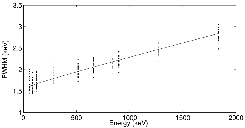
Figure 1: Spectral resolution (FWHM) for the flight model camera at 90 K. For each energy, the resolutions for the 19 individual detectors are plotted. The fit function is given by Eq. (2).

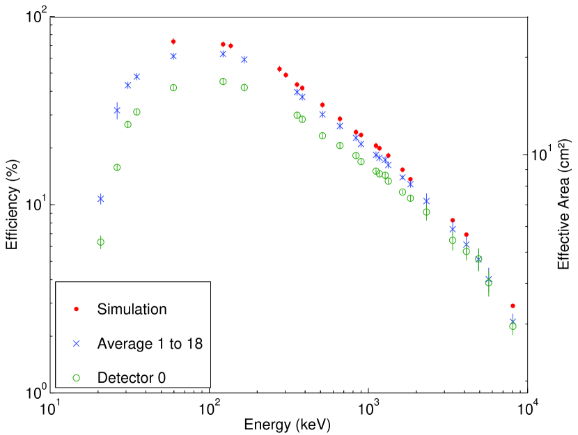
Figure 2: Full-energy peak efficiency for sources on the SPI optical axis ($\alpha=0^{\circ}$), without mask. An average for detectors 1 to 18 is shown; detector 0 is plotted separately (see Sec. 5.2). The measurements are compared to Monte-Carlo simulations.

5 Full-energy peak efficiency of the SPI telescope

To obtain the full-energy peak efficiency of the SPI telescope we corrected the efficiency of the camera alone for the absorption of photons by the mask. These results are compared to simulations.

Figure 3: For each detector, a plot of the efficiency versus energy is shown (in each plot, the line energy increases from left to right according to the 14 energies used). The crosses represent the mass of the crystal. When the detector is not shadowed, the efficiency depends mainly on its mass. Left panel: at $0^{\circ}$, source on axis, the detectors 0,2 and 3 are partially shadowed by the PSAC-alignment device. Right panel: when the source is at $8^{\circ}$, detectors 16 to 18 are shadowed by the ACS. The alignment device is projected outside the detection plane.

5.1 Individual detector efficiencies

For a Ge detector $i$, and a $\gamma$-ray line at energy E produced by a source, the full-energy peak efficiency $\epsilon_{i}$ is defined by the ratio

$$\epsilon_{i}=\frac{\phi_{\rm measured}}{\phi_{\rm incident}}$$ (3)

where $\phi_{\rm measured}=\mathcal{A}/T_{\rm m}$. $\mathcal{A}$ is the number of photons in the photopeak. We consider $\mathcal{A}$ to be the integral of the Gaussian part of the function $F(x)$ fitted to the background subtracted photopeak ($\mathcal{A}=\sqrt{2\pi}N\sigma$). $T_{\rm m}$ is the effective measurement duration (i.e. the total duration of the measurement corrected for the dead time).

In the case of a source, the absolute flux $\phi_{\rm incident}$ at the detector plane is given by

$$\phi_{\rm incident}=a_{0}\times 2^{-\frac{T_{1}-T_{0}}{\tau}}\times{\cal B}r_{E}\times\Omega\times e^{-\frac{\mu_{\rm E}}{\rho}x}$$ (4)

where $a_{0}$ is the source activity at the reference date $T_{0}$, $T_{1}$ is the date of the measurement and $\tau$ the half-life of the source, ${\cal B}r_{E}$ is the branching ratio of the line at energy E. The air transmission coefficient is computed using the air mass attenuation coefficient $\mu_{E}$ at energy E, the air density $\rho$ and the distance $x$ between the source and the Ge detection plane. $\Omega$ is the relative area of the detector viewed from the source $\Omega\leavevmode\nobreak\ =\frac{A_{\rm Ge}}{4\pi\times x^{2}}$ where $A_{\rm Ge}$ is the geometric area of a Ge detector, $\langle A_{\rm Ge}\rangle=26.75$ cm².

For the accelerator case, the intensities ${\cal I}r_{E}$ of the lines in the accelerator spectrum, corrected for all absorption effects, are relative to the 1638 keV line intensity (Tab. 2). The efficiency is:

$$\epsilon_{i}(E)=\frac{\phi_{\rm measured}(E)}{{\cal I}r_{E}\times\phi_{\rm measured}(1638)}\times\epsilon_{i}^{\rm{int}}(1638)$$ (5)

where $\epsilon_{i}^{\rm{int}}(1638)$ is the detector efficiency at 1638 keV obtained from the interpolation of source data.

For detectors 1 to 18, efficiencies are comparable. The value $\langle\widetilde{\epsilon}\rangle=\frac{1}{18}\sum_{i=1}^{\leavevmode\nobreak\ 18}\epsilon_{i}$ is representative of the efficiency of a single detector. Efficiencies $\epsilon_{0}$ and $\langle\widetilde{\epsilon}\rangle$ are compared to the GEANT simulation average efficiency $\langle\widetilde{\epsilon}\rangle_{\rm sim}$. $\langle\widetilde{\epsilon}\rangle_{\rm sim}$ is $\sim$10 % higher than $\langle\widetilde{\epsilon}\rangle$ (Fig. 2).

5.2 Homogeneity of the camera

Using 14 of the 18 energies of Tab. 1, we compared for each detector i the efficiency homogeneity functions $h_{i}(E)=\big{[}\frac{\epsilon_{i}-\langle\widetilde{\epsilon}\rangle}{\langle\widetilde{\epsilon}\rangle}\big{]}_{E}$ to the corresponding mass homogeneity functions $M_{i}\leavevmode\nobreak\ =\leavevmode\nobreak\ \frac{m_{i}-\langle m\rangle}{\langle m\rangle}$ where $\langle m\rangle=\frac{\Sigma_{i}^{n}m_{i}}{n}$. In Fig. 3 we display the homogeneity functions and their energy dependence for sources for a range of energies $E$ on the optical axis ($\alpha=0^{\circ}$) and for $\alpha=8^{\circ}$.

If $\alpha=0^{\circ}$, the efficiency of detector 0 seems to be $\sim$ 10 to 20 % less than $\langle\widetilde{\epsilon}\rangle$, and the deviation increases when the energy decreases. This behaviour is the signature of absorption, which in the case is due to an Hostaform plastic device inserted in the center of the plastic anticoincidence scintillator (PSAC) for alignment purposes. Detectors 2 and 3 are also affected. It was subsequently found that during these calibration runs the sources were actually slightly off-axis, causing the alignment device to partially shadow detectors 2 and 3. This explains the slight attenuation observed for them (Fig. 3, left panel).

If $\alpha\neq 0^{\circ}$, the alignment device is projected on one or more other detector(s). During measurements at $\alpha=8^{\circ}$, it is projected outside the camera, detector 0 shows a normal efficiency. The very low efficiency of detectors 16 to 18 is due to the shadow of the ACS (Fig. 3, right panel).

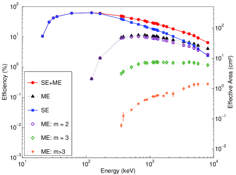
Figure 4: Full-energy peak efficiency for SE, ME and all events (SE+ME) and for ME with multiplicity m = 2, 3 and $>3$, for the camera without mask. The effective area is the geometric area multiplied by the efficiency.

5.3 Full-energy efficiency of the camera for the Multiple Events (ME)

In the case of ME, the incoming photon cannot be associated with a specific detector. So, the whole camera must be considered. We constructed a spectrum for each calibration source and multiplicity $m$ using events from the whole camera. We then fit the lines in the background corrected spectra. The ME efficiency for a multiplicity $m$, $\epsilon_{\rm ME}^{m}$, is defined as for the SE in Eq. (3). We find that above $\sim$4 MeV, the total ME efficiency is greater than the SE efficiency. The contribution of different multiplicities is displayed in Fig. 4.

5.4 Full-energy peak efficiency of the telescope

During the acquisition of the data used in the previous sections, the mask was removed to let all detectors be illuminated by the sources. Deriving the telescope efficiency from the camera and detector efficiencies need to be corrected for the absorption of photons by the open and closed elements of the mask. This correction is evaluated for on-axis sources at infinite distance, thus the rays are considered to arrive parallel on the mask.

The transparency of the 63 open mask pixels have been measured individually with different radioactive sources from 17 keV to 1.8 MeV (Sánchez et al. (2003)). Using these data, a mathematical model was fit to reproduce the mask absorption for the open pixels and especially for the central pixel, affected also by the alignment device. Note that above 2 MeV the absorption values have been extrapolated.

The efficiencies computed from on-axis 8-meter source data analyses for the detectors 0 and 3 were corrected for absorption due to the mask support (Fig. 5). For detector 3, these efficiencies are in good agreement with the efficiencies obtained with the mask installed at ESTEC and at BLC using the 125-meter source data. Thus, for an unshadowed detector, the correction method can be applied. For detector 0, when the source is on axis, the presence of the alignment devices in the PSAC and the mask complicates the efficiency calculation. Below 1 MeV, we adjusted the correction (Sánchez et al. (2003)) to fit the BLC and ESTEC measurements.

Let $M_{\circ}(E)$ be the mask support transmission for the illuminated detectors, $M_{\bullet}(E)$ the mask element transmission multiplied by the mask support transmission for the shadowed ones. For SE, $M_{i}(E)$ is the transmission of the element i of the mask at the energy $E$ for the detector $i$ ($M_{i}(E)=M_{\circ}(E)$ or $M_{\bullet}(E)$). For SE we correct the efficiency for each detector. For ME we correct the global camera efficiency obtained in Sec 5.3 by the global mask absorption. The total effective area $\mathcal{A}_{\rm eff}$ of the telescope is then:

$$\mathcal{A}_{\rm eff}=\sum_{\rm i=0}^{\rm 18}\mathbf{A}_{i}^{SE}(E)\times M_{i}(E)$$

$$\leavevmode\nobreak\ \leavevmode\nobreak\ \leavevmode\nobreak\ \leavevmode\nobreak\ \leavevmode\nobreak\ \leavevmode\nobreak\ \leavevmode\nobreak\ \leavevmode\nobreak\ +\mathbf{A}^{ME}(E)\times\Big{[}\frac{\mathbf{A}_{\bullet}}{\mathbf{A}}M_{\bullet}(E)+\frac{\mathbf{A}_{\circ}}{\mathbf{A}}M_{\circ}(E)\Big{]}\$$ (6)

$\mathbf{A}_{i}^{SE}(E)$ is the effective area of detector $i$ for the SE, $\mathbf{A}^{ME}(E)$ is the camera effective area for the ME. $\mathbf{A}_{\circ}$, $\mathbf{A}_{\bullet}$ and $\mathbf{A}$ are the total geometric area of the illuminated detectors, of the shadowed detectors and of the whole camera. In the case of a source on axis at infinity, $\mathbf{A}_{\circ}=240.9\leavevmode\nobreak\ \rm cm^{2}$, $\mathbf{A}_{\bullet}=267.4\leavevmode\nobreak\ \rm cm^{2}$ and $\mathbf{A}=508.3$ cm².

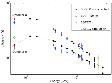
Figure 5: The on-axis, full-energy peak efficiencies of detector 0 and 3 for SPI with its mask. The data are: 8 m BLC data without mask corrected for the mask absorption ($\cdot$), 125 m BLC data with mask, ($\circ$) and 8 m ESTEC data with mask ($\times$). For detector 0, the disagreement between the curves shows the difficulty of alignment device modelisation.

For imaging, Eq. (6) is not fully valid for ME. In this case, the number of the detector where the photon had its first interaction can be known only with a probability $p<1$. The $(1-p)$ fraction is attributed to other pixels of the mask (closed or open), and so the real ME efficiency is always less than (ME  camera  efficiency) $\times$ (mask  absorption  corrections).

We have compared the measured effective areas of the SPI telescope to those found in the SPI Imaging Response Files (IRFs), see Fig. 6. Here we have limited our comparison to the on-axis full-energy peak effective areas. The IRFs used in the ISDC data analysis pipeline have been simulated using a GEANT-based software package (Sturner et al. (2003)). Note that the version of the IRFs released in November 2002 have subsequently been corrected at low energies using calibration data. The total effective area is about 125 cm² at 100 keV and 65 cm² at 1 MeV.

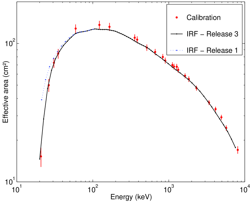
Figure 6: Full-energy peak effective area of SPI telescope using all events (SE+ME). This curve is representative of the in flight effective area for an on-axis source. We compare it to the response matrix before the launch (release 1, nov 2002) and after the launch (release 3, july 2003).

6 Imaging Capabilities

The long-distance source tests were designed to verify the capabilities of the entire instrument in the imaging mode, the response matrix derived from Monte Carlo simulations, and the performance of the instrument/software/response matrix combination. For 125 m, the beam divergence was about $\pm 4^{\prime}$ and the angular size of the sources $\sim 1^{\prime}$.

6.1 Angular resolution and Point Spread Function

The angular resolution and Point Spread Function (PSF) of an instrument such as SPI is a function not only of the characteristics of the instrument but of the sequence of pointings (the “dithering pattern”) used and the image reconstruction technique adopted. Here we take the PSF to be the response in an image obtained by correlation mapping (Skinner & Connell (2003)) to a point source observed according to a specific dither pattern. We then take as the angular resolution the full width at half maximum (FWHM) of this response. Fig. 7 shows some results.

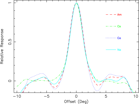
Figure 7: The PSF determined from measurements of 4 different sources at 125 m. Each curve is the mean of cross-sections through the response in two orthogonal directions; a background level has been subtracted from each and the curves normalized to the same peak height. The mean FWHM is 2.55^∘. (²⁴¹Am: 60 keV; ¹³⁷Cs: 662 keV; ⁶⁰Co: 1332 keV; ²⁴Na: 2754 keV)

Given that the hexagonal mask elements are 60 mm “across flats” and that the mask-to-detector distance is 1710 mm, the expected angular resolution is 2.0^∘. But because of the finite detector spatial resolution, the FWHM will be larger. Although the detector pitch is equal to the mask element size, the detectors are somewhat smaller (56 mm). This gives an expected FWHM of about 2.5^∘. The measured values are consistent with predictions. The FWHM does not vary significantly with energy for the sources used (59–2754 keV).

Figure 8: The error in the determination of a narrow line source position from analysis of calibration data. Squares: subsets of data, circles: mean of 10–20 trials with samples of random noise added. Open symbols: deviations from the nominal position, filled symbols: deviations from an assumed displaced source position. The line corresponds to 2.5^∘$/N_{\sigma}$.

6.2 Single source localisation precision

The source location accuracy depends on the signal-to-noise ratio, $N_{\sigma}$, of the measurement as well as the angular resolution of the instrument. Some analysis results of the analysis software Spiros (Connell et al. (1999), Skinner & Connell (2003)) are shown in Fig. 8. The signal-to-noise ratio of the BLC data is extremely high. It is important to verify the performances with values of $N_{\sigma}$ more representative of flight values. To do this, random subsets of events were taken. These subset were also diluted by adding increasing amounts of Poisson-distributed noise. We found that the position accuracy does not increase when the signal-to-noise ratio exceeded 50-100$\sigma$. This suggests that there are systematic effects, which limit the accuracy to $>2.5^{\prime}$. This could be due to uncertainties in the telescope stand alignment, which are about that level. Assuming that the reference axis was displaced from the source direction by a fixed 2.5^′, the residual errors suggest that the intrinsic limit of the instrument may be about five times lower (filled symbols).

6.3 Source separation capability

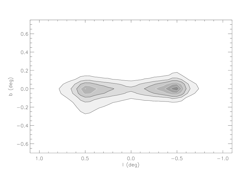
Figure 9: Maximum entropy image in the 1173 keV ⁶⁰Co line shows the capability of the instrument to separate sources closer than the angular resolution, where the signal-to-noise ratio is good. The sources are separated by 1^∘.

Even if the angular resolution is about 2.5^∘, one can distinguish sources separated by less than this angle if data have a good signal-to-noise ratio. The BLC calibration runs were restricted to single sources, but it is possible to combine the data from runs at different source angles to emulate data for double sources. Fig. 9 shows Spiskymax (Strong (2003)) image for sources separated by 1^∘using the 1173 keV line of ⁶⁰Co. The source are clearly separated, thus showing that SPI, in the very high signal-to-noise regime of BLC, is able to resolve sources at least as closely spaced as 1^∘. With the lower signal-to-noise flight conditions the same performance will not always be achieved.

7 Anti-Coincidence System performance

A threshold calibration was performed using two radioactive sources (²⁰³Hg: 279 keV; ¹³⁷Cs: 662 keV) placed close to each of the 91 BGO crystals. The redundant cross-connections between pairs of crystals, PMTs (photomultiplier tube) and electronics give a broad threshold function, which can be approximated by

$$s(E,E_{\rm th})=\frac{1}{\sigma(E)\times\sqrt{2\pi}}\times\int_{E_{\rm th}}^{+\infty}{e^{-\frac{(E\leavevmode\nobreak\ ^{\prime}-E)^{2}}{2\sigma^{2}(E)}}dE\leavevmode\nobreak\ ^{\prime}}$$ (7)

where s is the probability that a $\gamma$-ray with energy E exceeds the threshold energy E_th. A relation $\sigma(E)=a\times\sqrt{E}$ has been assumed (Fig. 10).

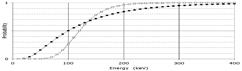
Figure 10: For PMT₁(solid), $E_{\rm th}$ = 100 keV and $a=\sqrt{50}$, for PMT₂(open), 120 keV and $\sqrt{10}$. These curves illustrate the large differences between ACS crystals and PMTs combinations.

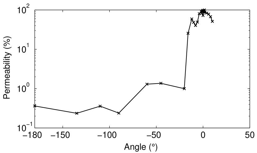
Figure 11: ACS permeability as a function of the angle from the axis (BLC, ¹³⁷Cs source)

The light yield of BGO crystals varies with the temperature. This has an significant effect on two main characteristics of the ACS:

• the self-veto effect is the rejection of true source counts by the anticoincidence shield, due to Compton leakage from the camera. It decreases when the ACS threshold energy raises as more scattered events are accepted. For a detector located on the edge of the camera, the influence is larger than for an inner one.

• the veto-shield permeability is the fraction of $\gamma$-rays, which go through the ACS shield undetected and then hit a Ge detector. If a strong source is outside the field of view, it will be imaged through the structure of the veto shield, which will act as a kind of mask (Fig. 11).

These two ACS effects will modify the in-flight sensitivity of the telescope: variations of temperature on the orbit will affect the Compton background under the lines and the dead time. Current in-flight variations are about 10 K. They are permanently monitored so that these effects could be further quantified.

8 Background lines

We produced a catalogue of all the $\gamma$-ray lines detected by SPI on the ground (Tab. 3) by summing over all of the background data. Some never before observed very-high energy lines were detected. These lines are also visible in the E_p = 1747 keV spectra, but not in the E_p = 550 keV ones. A careful study of BLC environment excluded any kind of non-natural emission during our background tests. A complementary test of $3\times 10^{5}$ s using an isolated standard Ge detector did not produce these lines. So their observation in the SPI background spectra must be related to the presence of low energy or thermal neutrons and the Ge detector array structure of the camera.

During background measurements, the neutron flux comes mainly from the spallation of SPI materials by cosmic rays. Thermal neutron capture for Ge isotopes has been studied in details by Islam et al. (1991). They give the neutron separation energies: $S_{n}(^{71}$Ge$)=7415.9$ keV, $S_{n}(^{74}$Ge$)=10196.3$ keV, $S_{n}(^{75}$Ge$)=6505.2$ keV. Lines are detected in SPI at these energies, but the most striking feature is that the 10196 keV line corresponds to a forbidden transition between the S_n level and the ground state.

A simulation of some of the numerous possible cascades in the de-excitation of ⁷⁴Ge nuclei showed that such a line can only be observed due to the summation of different transitions of the cascade by at least two detectors close to one another, i.e. in coincidence. On the other hand, the line corresponding to $S_{n}(^{73}$Ge$)=6782.9keV$ is not observed, but a 6717 line is. This line corresponds also to the summation of transitions, but only down to the 67 keV level of the isomeric ^73mGe which decays independently with a lifetime of 0.499 s.

The determination of line origins is necessary to understand the SPI camera behaviour in space, where neutron and spallation induced lines will affect the observations. The relative intensities obtained in the ground calibration can then be used when subtracting the background from astrophysical data.

9 Conclusion

SPI will be able to detect nuclear astrophysics lines and continuum. The total effective area of SPI was found to be $>100$ cm² in the energy range 40 keV to 300 keV with a maximum of 136 cm² at 125 keV. At 1 MeV the resolution of the instrument is $\sim$2.5 keV with an effective area of $\sim$65 cm². (At 511 keV: 90 cm²; At 1.8 MeV: 52 cm²).

The angular resolution of SPI was found to be roughly 2.5^∘and it has been shown that SPI will be able to resolve sources with a separation of 1^∘and probably less.

Using ground calibration data and GEANT simulations, we derived an absolute calibration of the SPI effective area. We noticed the temperature influence on ACS effects and energy restitution. For these two points, we must underline that permanent in-flight calibration is required. Neutron or spallation induced background lines will be used as tracers to extract the background component of some lines of astrophysical interest.

E (keV)	Source	$\epsilon_{\rm SE}$ (%)	$\epsilon_{\rm ME}$ (%)	$T_{\rm ms}$ (%)	$T_{\rm cp}$ (%)	$A_{\rm eff}$ (cm2)	$\Delta A_{\rm eff}$ (cm2)
20.80	241Am	10.5	0.0	57.1	30.2	15.3	1.4
26.35	241Am	30.8	0.0	63.6	36.6	50.0	4.2
30.80	133Ba	42.2	0.0	67.2	40.8	72.5	5.7
35.07	133Ba	47.0	0.0	70.1	44.3	84.4	6.4
59.54	241Am	60.4	0.0	82.1	59.5	128.1	8.6
122.06	57Co	62.2	0.4	83.7	66.1	136.2	8.9
165.86	139Ce	58.1	2.0	84.4	68.9	131.9	8.4
356.02	133Ba	39.1	9.5	86.1	75.9	110.0	5.9
383.85	133Ba	36.9	10.1	86.3	76.6	106.6	5.6
514.01	85Sr	29.8	10.9	86.9	79.2	93.3	4.7
661.7	137Cs	25.9	11.5	87.5	81.6	86.7	4.2
834.84	54Mn	22.4	11.4	88.0	83.7	79.8	3.8
898.04	88Y	20.8	10.9	88.1	84.3	75.2	3.5
1115.55	65Zn	18.2	10.6	88.6	86.3	69.8	3.2
1173.24	60Co	17.6	10.3	88.7	86.8	68.0	3.1
1274.5	22Na	17.1	10.4	88.9	87.6	67.9	3.0
1332.5	60Co	16.1	10.0	89.0	88.0	64.4	2.9
1836.06	88Y	12.7	8.9	89.7	90.9	55.3	2.4

Table 1: Energies of the radioactive sources used at 8.533 meters and the associated efficiency calibration obtained at Bruyères-Le-Châtel. The efficiencies camera for the SE and ME is respectively given by $\epsilon_{\rm SE}$ and $\epsilon_{\rm SE}$. The transparency of the mask support is $T_{\rm ms}$ and the transparency of the central pixel is $T_{\rm cp}$. Using this transmission factors and with an air density $\rho=1.205\times 10^{-3}$ g cm^-3 the effective area of the SPI telescope is given by $A_{\rm eff}$ with the error $\Delta A_{\rm eff}$ in cm².

Eγ (keV)	${\cal I}_{0}$	${\cal I}r_{\rm E}$	$\epsilon_{\rm SE}$ (%)	$\epsilon_{\rm ME}$ (%)	$T_{\rm ms}$ (%)	$T_{\rm dev}$ (%)	$A_{\rm eff}$ (cm2)	$\Delta A_{\rm eff}$ (cm2)
1637.9	100	100	13.8	9.3	89.5	89.8	58.4	2.3
2316	139 $\pm$ 4.3	149 $\pm$ 4.6	10.4	7.9	90.2	93.0	47.6	1.8
3383.8	23.7 $\pm$ 0.8	27.0 $\pm$ 0.9	7.4	6.8	91.1	96.5	37.4	1.4
4123	102 $\pm$ 3.2	119 $\pm$ 3.7	6.1	6.5	91.5	98.3	33.5	1.2
4922.8	16.3 $\pm$ 0.6	19.1 $\pm$ 0.7	5.1	5.9	91.9	99.9	29.3	1.1
5700.1	12.8 $\pm$ 0.5	15.1 $\pm$ 0.6	4.0	5.2	92.2	99.9	24.5	1.0
8076	627 $\pm$ 20	752 $\pm$ 24	2.4	4.1	93.0	99.9	17.0	0.7

Table 2: Strongest $\gamma$-ray lines of the 550 keV resonance of the ¹³C(p,$\gamma$)¹⁴N reaction. ${\cal I}_{0}$ is the relative intensity emitted by the target under 45^∘, ${\cal I}r_{\rm E}$ is the relative intensity at SPI position after absorption in the target backing and holder, the cooling water, 8 m of air and the window separating SPI from the experimental hall (normalized to the 1637.9 keV line). The 8076 keV line is Doppler shifted from its nominal 8060 keV, as all lines coming from the 8062 keV level. For the others values see Tab. 1.

Energy	Nuclide	Emission	Half-life	Others gammas	Origin	Fluxes
(keV)		probability (%)		(keV) (%)		(s-1)
46.5	210Pb	4.05	22.3 y		238U series (226Ra)	0.276
59.5	241Am	36.0	432.2 y			0.094
63.3	234Th	4.5	24.1 d		238U series (226Ra)	0.365
66.7	73mGe	100	0.499 s		activation	-
72.8	Pb X-ray	[100]		75.0[100]	fluorescence K$\alpha 1$	0.765
75.0	Pb X-ray	[60]		72.8[60]	fluorescence K$\alpha 2$	0.822
75.0	208Tl	3.6	3.053 m	2614.6(99.8)	fast neutron activation	0.822
84.8	208Tl	1.27	3.053 m	2614.6(99.8)	fast neutron activation	-
84.9	Pb X-ray	[35]		75.0[100]	fluorescence K$\beta 1$	-
87.3	Pb X-ray	[8.5]		75.0[100]	fluorescence K$\beta 2$	-
93.3	228Ac	5.6	6.15 h	911.2(29.0)	232Th series	0.696
143.8	235U	10.9	7$\times 10^{8}$ y	185.7(57.2)	natural	0.132
162.7	235U	4.7	7$\times 10^{8}$ y	185.7(57.2)	natural	0.090
185.7	235U	57.2	7$\times 10^{8}$ y	143.8(10.9)	natural	0.835
186.1	226Ra	3.28	1600 y		238U series	0.835
198.3	73mGe	100	0.499 s		activation	0.033
205.3	235U	4.7	7$\times 10^{8}$ y		natural	0.086
209.4	228Ac	4.1	6.15 h	911.2(29.0)	232Th series	-
238.6	212Pb	43.6	10.6 h	300(3.34)	232Th series	0.753
240.8	224Ra	3.9	3.66 d		232Th series	-
269.4	223Ra	13.6			235U series	0.014
270.3	228Ac	3.8			232Th series	-
295.1	214Pb	19.2	26.8 m	3351.9(35.1)	238U series (226Ra)	0.176
300.0	212Pb	3.34	10.6 h	238.6(43.6)	232Th series	0.044
338.4	228Ac	12.4	6.13 h	911.2(29)	232Th series	0.124
351.9	214Pb	37.1	26.8 m	285.1(19.2)	238U series (226Ra)	0.323
409.6	228Ac	2.2	6.15 h	911.2(29.0)	232Th series	-
432.8	212Bi	6.64	1.1 h	727.2(6.65)	232Th series	-
463.1	228Ac	4.6	6.15 h	911.2(29.0)	232Th series	0.011
510.8	208Tl	22.8	3.053 m	2614.6(99.8)	232Th series	-
511.0	many				annihilation $e^{+}/e^{-}$	-
569.6					-	0.125
583	208Tl	84.5	3.053 m	2614.6(99.8)	232Th series	0.100
609.3	214Bi	46.1	19.9 m	1120.3(15.0)	238U series (226Ra)	0.137
661.7	137Cs	85.1	30.17 y		-	0.016
665.5	214Bi	1.55	19.9 m	609.3(46.1)	238U series (226Ra)	0.015
726.8	228Ac	0.62	6.13 h	911.2(29)	232Th series	-
727.2	212Bi	6.65	1.1 h	1620.7(1.51)	232Th series	0.085
755.3	228Ac	1.32	6.13 h	911.2(29)	232Th series	0.008
766.4	214Bi	4.83	19.9 m	609.3(46.1)	fission (95Zr)	0.066
766.4	234Pa	0.29	0.79 s	1001.0(0.83)	238U series	0.125
784.0	127Sb	14.5	3.85 d	685.7(35.3)	fission	0.032
794.8	228Ac	4.6	6.13 h	911.2(29)	232Th series	0.021
834.8	54Mn	99.98	312.3 d		charged particle reaction	0.023
860.6	208Tl	12.52	3.053 m	2614.6(99.8)	232Th series	0.025
904.3	214Bi	0.1	19.9 m	609.3(46.1)	238U series (226Ra)	0.318
904.3	228Ac	0.89	6.13 h	911.2(29)	232Th series	0.318
911.2	228Ac	29.0	6.13 h	969.0(17.4)	232Th series	0.320
934.1	214Bi	3.1	19.9 m	609.3(46.1)	238U series (226Ra)	0.014
964.6	228Ac	5.8	6.13 h	911.2(29)	232Th series	0.225
969	228Ac	17.4	6.13 h	911.2(29)	232Th series	0.259
1001.0	234Pa	0.83	0.79 s	766.4(O.29)	238U series	-
1063.6					-	0.059
1120.3	214Bi	15	19.9 m	609.3(46.1)	238U series (226Ra)	0.107
1155.2	214Bi	1.7	19.9 m	609.3(46.1)	238U series (226Ra)	0.011
1237	214Bi	5.96	19.9 m	609.3(46.1)	238U series (226Ra)	0.043
1281	214Bi	1.48	19.9 m	609.3(46.1)	238U series (226Ra)	0.010
1292					-	0.004
1377	214Bi	4.15	19.9 m	609.3(46.1)	238U series (226Ra)	0.050
1401.5	214Bi	1.39	19.9 m	609.3(46.1)	238U series (226Ra)	0.010
1408	214Bi	2.51	19.9 m	609.3(46.1)	238U series (226Ra)	0.020
1460.8	40K	10.67	1.289 y	-	natural	2.056
1492					-	0.015
1496	228Ac	1.05			232Th series	0.009
1508						0.027
1580	228Ac	0.71			232Th series	0.012
1764.5	214Bi	16.07			238U series (226Ra)	0.229
2614.4	208Tl	99.79	3.053 m	2614.6(99.8)	232Th series	0.545
3197.0	208Tl		3.053 m	2614.6(99.8)	232Th series	0.011
3475	208Tl		3.053 m	2614.6(99.8)	232Th series
3708.1	208Tl		3.053 m	2614.6(99.8)	232Th series	$<$0.001
6129.2	16O				-	$<$0.001
6505.2	75Ge				74Ge(n,$\gamma$)	$<$0.001
6716.5	73Ge				72Ge(n,$\gamma$)	$<$0.001
7415.9	71Ge				70Ge(n,$\gamma$)	0.001
7631.7	57Fe				56Fe(n,$\gamma$)	$<$0.001
7645.5	57Fe				56Fe(n,$\gamma$)	$<$0.001
10196	74Ge				73Ge(n,$\gamma$)	$<$0.001

Table 3: Background environment lines observed by SPI in absence of sources.