Weak Lensing and CMB: Parameter forecasts including a running spectral index

Abstract

We use statistical inference theory to explore the constraints from future galaxy weak lensing (cosmic shear) surveys combined with the current CMB constraints on cosmological parameters, focusing particularly on the running of the spectral index of the primordial scalar power spectrum, $\alpha_{s}$. Recent papers have drawn attention to the possibility of measuring $\alpha_{s}$ by combining the CMB with galaxy clustering and/or the Lyman-$\alpha$ forest. Weak lensing combined with the CMB provides an alternative probe of the primordial power spectrum. We run a series of simulations with variable runnings and compare them to semi-analytic non-linear mappings to test their validity for our calculations. We find that a “Reference” cosmic shear survey with $f_{sky}=0.01$ and $6.6\times 10^{8}$ galaxies per steradian can reduce the uncertainty on $n_{s}$ and $\alpha_{s}$ by roughly a factor of 2 relative to the CMB alone. We investigate the effect of shear calibration biases on lensing by including the calibration factor as a parameter, and show that for our Reference Survey, the precision of cosmological parameter determination is only slightly degraded even if the amplitude calibration is uncertain by as much as 5%. We conclude that in the near future weak lensing surveys can supplement the CMB observations to constrain the primordial power spectrum.

I Introduction

The recent observations of the cosmic microwave background (CMB) from the Wilkinson Microwave Anisotropy Probe (WMAP) mission confirmed the standard cosmological model to a very high degree of accuracy Spergel et al. (2003). The WMAP data alone is consistent with a spatially flat model dominated by dark energy and dark matter, with nearly scale-invariant, adiabatic and Gaussian initial perturbations consistent with the simplest inflationary models Guth (1981); Linde (1982); Albrecht and Steinhardt (1982).

One of the remaining outstanding issues is whether the shape of the primordial power spectrum is consistent with the theoretical predictions. This is usually expressed in terms of the slope of the primordial scalar spectrum $n_{s}$ and its running $\alpha_{s}=dn_{s}/d\ln k$. Most of the existing models predict that the slope is close, but not identical, to scale invariant, $n_{s}\sim 1$, and that running is small, $\alpha_{s}\sim(1-n_{s})^{2}$. The best way to observationally settle this question is by combining data over a wide range of scales. Combining data from WMAP, the Cosmic Background Imager (CBI) Pearson and Cosmic Background Imager Collaboration (2002), and the Arcminute Cosmology Bolometer Array Receiver (ACBAR) Kuo et al. (2002), together with constraints from the Two Degree Field Galaxy Redshift Survey (2dFGRS) Colless et al. (2001) Ref. Spergel et al. (2003) found 0.05 error on $n_{s}$ and 0.025 on $\alpha_{s}$, with scale invariant model fitting the data at 1.3 $\sigma$. Ref. Spergel et al. (2003) added Lyman-$\alpha$ forest constraints from Croft et al. (2002); Gnedin and Hamilton (2002) and reduced the error on running to 0.016 (as well as found evidence for running at $1.9\sigma$), but Ref. Seljak et al. (2003) showed that the assumed errors were too small and the current Lyman-$\alpha$ forest constraints do not add significantly to the constraints from the CMB. The constraints on $\alpha_{s}$ in Spergel et al. (2003) were obtained assuming no tensor modes, the strong degeneracy between running and tensors in the current data complicates the interpretation of the one-dimensional marginalized probability distribution for $\alpha_{s}$ Seljak et al. (2003). Other authors Bridle et al. (2003); Leach and Liddle (2003); Barger et al. (2003); Kinney et al. (2003) who did not use Lyman-$\alpha$ forest, also find no significant evidence for a running spectral index, with errors at the level of 0.03.

While the current data show no evidence for running, the errors are still large and will be improved in the future. The most immediate improvement will come from the Sloan Digial Sky Survey (SDSS)York et al. (2000). The galaxy power spectrum analysis is not expected to improve the 2dF results in a statistical sense (but will be an important check of systematics), since on scales smaller than a few Mpc the nonlinear bias becomes intractable. On the other hand, the Lyman-$\alpha$ forest spectrum and bispectrum analysis of several thousand quasar spectra in SDSS will lead to an order of magnitude improvement of the Lyman-$\alpha$ constraints Mandelbaum et al. (2003). In combination with the CMB this is expected to give an error of $5\times 10^{-3}$ on $\alpha_{s}$.

There are however uncertanties associated with the baryonic physics of the Lyman-$\alpha$ forest. Future high-$\ell$ CMB data from the Planck satellite (and, to a lesser extent, measurement of the second and third acoustic peaks from future WMAP data) will enable precision measurement of $\alpha_{s}$ independently of the galaxy and Lyman-$\alpha$ data, but contamination from secondary anisotropies and foregrounds at high $\ell$ may be significant, since we are interested in effects of only a few percent. (The measurement of the first acoustic peak by WMAP is comparatively clean due to the large cosmological signal.)

It is therefore desirable to have yet another probe of the primordial power spectrum at high wavenumbers. Weak lensing is an attractive candidate since most of the potential systematics are related to the difficulty of the observations and are unrelated to the systematics associated with the other cosmological probes we have discussed. The purpose of this paper is to explore the constraints from future galaxy weak lensing (cosmic shear) surveys combined with the current CMB results on cosmological parameters, particularly the running of the scalar spectral index. Weak lensing is one of the most promising tools for an era of precision cosmology as it probes directly the distribution of the gravitating matter and does not suffer from the uncertainties associated with nonlinear bias or gas physics (for reviews, see Refregier (2003); Bartelmann and Schneider (2001); Mellier (1999) and references therein).

A few authors have used statistical inference theory to report forecasts on how well cosmic shear surveys combined with CMB data are able to constrain cosmological parameters. See, for example Hu and Tegmark (1999); Hu (2002). Our goal is to extend these studies to include the running, as well as investigate the effects of possible systematics on the results. More recently, Refs. Contaldi et al. (2003); Wang et al. (2002) combined CMB data from various experiments with the Red-Sequence Cluster Survey (RCS) weak lensing survey data (53 deg²) Hoekstra et al. (2002a, b). Even with a modest survey, they found that their analysis reduces the uncertainties by comparable amounts or better than when the CMB results are combined with other types of probes because it breaks degeneracies present in the CMB data. Their results are consistent with the earlier forecasts. Other recent papers that reported statistical forecasts on how well weak lensing will be able to constrain various cosmological parameters include Huterer (2002); Abazajian and Dodelson (2003); Benabed and Van Waerbeke (2003); Takada and Jain (2003); Takada and White (2003); Heavens (2003); Jain and Taylor (2003); Bernstein and Jain (2003); Simon et al. (2003).

The potential of weak lensing as a cosmological probe has been realized quickly and there are many ongoing, planned, and proposed surveys, such as the Deep Lens Survey (http://dls.bell-labs.com/) Wittman et al. (2002); the NOAO Deep Survey (http://www.noao.edu/noao/noaodeep/); the Canada-France-Hawaii Telescope (CFHT) Legacy Survey (http://www.cfht.hawaii.edu/Science/CFHLS/) Mellier et al. (2001); the Panoramic Survey Telescope and Rapid Response System (http://pan-starrs.ifa.hawaii.edu/); the Supernova Acceleration Probe (SNAP; http://snap.lbl.gov/) Rhodes et al. (2003); Massey et al. (2003); Refregier et al. (2003); and the Large Synoptic Survey Telescope (LSST; http://www.lsst.org/lsst_home.html) Tyson (2002). In this paper we will discuss parameter constraints possible with a Reference Survey obtaining the shapes of $\bar{n}=6.6\times 10^{8}$ galaxies per steradian over a fraction $f_{sky}=0.01$ of the sky (413 deg²), with a peak redshift $z_{p}=1$. We also explore the effect of varying $f_{sky}$ and $\bar{n}$. The Reference Survey is somewhat more ambitious than the CFHT wide synoptic survey (172 deg²); roughly comparable to the SNAP wide survey; and significantly less ambitious than the LSST.

II Formalism and model

II.1 Model parameters

We consider the following basic parameter set for weak lensing: $\Omega_{m}h^{2}$, the physical matter density; $\Omega_{\Lambda}$, the fraction of the critical density in a cosmological constant; $n_{s}(k_{0})$ and $\alpha_{s}$, the spectral index and running of the primordial scalar power spectrum at $k_{0}$; $\sigma_{8}^{\rm lin}$, the amplitude of linear fluctuations; $z_{p}$, the characteristic redshift of the source galaxies (see Eq. 4); and $\zeta_{s}$ and $\zeta_{r}$, the calibration parameters (see §II.3). In order to combine this with information from the CMB we include $\Omega_{b}h^{2}$, the physical baryon density; $\tau$, the optical depth to reionization; $T/S$ the scalar-tensor fluctuation ratio. We assume a spatially flat Universe with $\Omega_{m}+\Omega_{\Lambda}=1$, thereby fixing $\Omega_{m}$ and $H_{0}$ as functions of our basic parameters, and we do not include dynamical dark energy, massive neutrinos, or primordial isocurvature perturbations. The primordial power spectrum of scalar density fluctuation is given by Kosowsky and Turner (1995)

$$P(k)=P(k_{0})\left(\frac{k}{k_{0}}\right)^{n_{s}(k_{0})+\frac{1}{2}\alpha_{s}\ln\left(\frac{k}{k_{0}}\right)},$$ (1)

where $n_{s}(k)\equiv\frac{d\ln P}{d\ln k}$ and $\alpha_{s}(k)\equiv\frac{d\ln n_{s}}{d\ln k}$. We assume $\frac{d^{2}\ln n_{s}}{d\ln k^{2}}=0$, i.e. we ignore higher-order terms in the Taylor expansion of the primordial power spectrum. We have taken our pivot wavenumber to be $k_{0}=0.05$ h/Mpc. We use as fiducial model the best fit for the WMAP(1yr)+ACBAR+CBI data from the Markov Chains in Ref. Seljak et al. (2003): $\Omega_{b}h^{2}=0.0228$, $\Omega_{m}h^{2}=0.139$, $\Omega_{\Lambda}=0.74$, $n_{s}=0.95$, $\alpha_{s}=0$ (with $\pm 0.04$ variations), $\sigma_{8}=0.85$, $\tau=0.177$, $T/S=0.265$, $z_{p}=1.0$, $\zeta_{s}=0.0$, and $\zeta_{r}=0.0$.

II.2 Convergence power spectrum

We use the Limber approximation to the convergence power spectrum Kaiser (1992); Jain and Seljak (1997); Kaiser (1998), which is valid on small angular scales $\ell\gg 1$ for which the gravitational lensing deflection can be approximated as a random walk due to many independent structures along the line of sight:

$$P_{\kappa}(\ell)=\frac{9}{4}H_{0}^{4}\Omega_{m}^{2}\int^{\chi_{H}}_{0}\frac{g^{2}(\chi)}{a^{2}(\chi)}P_{3D}\left(\frac{\ell}{\sin_{K}(\chi)},\chi\right)d\chi.$$ (2)

Here $P_{3D}$ is the $3D$ nonlinear power spectrum of the matter density fluctuation, $\delta\rho/\rho$; $\chi$ is the radial comoving coordinate; $a(\chi)$ is the scale factor; and $\sin_{K}\chi=K^{-1/2}\sin(K^{1/2}\chi)$ is the comoving angular diameter distance to $\chi$. The weighting function $g(\chi)$ is the source-averaged distance ratio given by

$$g(\chi)=\int_{\chi}^{\chi_{H}}n(\chi^{\prime}){\sin_{K}(\chi^{\prime}-\chi)\over\sin_{K}(\chi^{\prime})}d\chi^{\prime},$$ (3)

where $n(\chi(z))$ is the source redshift distribution normalized by $\int dz\;n(z)=1$.

For our weak lensing calculations, we used the BBKS linear transfer function Bardeen et al. (1986) appropriate for cold dark matter with adiabatic initial perturbations. No baryonic correction was applied, since $\Omega_{b}h^{2}$ is tightly constrained by the CMB and since the baryonic oscillations that appear in the full transfer function are smoothed out by projection effects when the convergence power spectrum is determined. We have used the analytic approximation to the growth factor of Ref. Lahav et al. (1991). We used the recent nonlinear mapping procedure halofit Smith et al. (2003) to compute the non-linear power spectrum. This procedure, as described in Smith et al. (2003), is based on a fusion of the halo model and an HKLM scaling Hamilton et al. (1991) and is more accurate than the commonly used Peacock-Dodds mapping Peacock and Dodds (1996). We discuss it further in section III and check it versus numerical simulations. We contrast in Fig. 1 two curved convergence power spectra for $\alpha_{s}=-0.04,0.04$ and display the sample variance errors averaged over bands in $\ell$ and the noise in the measurement.

Figure 1: Curved convergence power spectra for the Reference Survey with $\alpha_{s}=-0.04$ (solid curve) and $\alpha_{s}=0.04$ (dashed); $k_{0}=0.05h/Mpc$ and all other parameters are fixed at their fiducial values. The dotted line represent the noise power spectrum. The Reference Survey is sampling variance-limited out to $\ell\approx 2000$.

For $n(z)$, we take the fitting function Wittman et al. (2000):

$$n(z)=\frac{z^{2}}{2z_{0}^{3}}\,e^{-z/z_{0}},$$ (4)

which peaks at $z_{p}=2z_{0}$. When we consider tomography, the sources are split in two bins: $z<z_{p}$ and $z\geq z_{p}$. The normalized source redshift distributions for these two bins are:

$${n_{A}(z)=\frac{z^{2}}{2z_{0}^{3}(1-5/e^{2})}\,{e^{-z/z_{0}}}} {\;\;{\rm for}\;\;}{z_{p}<2z_{0}}$$

$${n_{B}(z)=\frac{e^{2}z^{2}}{10z_{0}^{3}}\,{e^{-z/z_{0}}}} \;\;{\rm for}\;\;{z_{p}\geq 2z_{0}}.$$ (5)

II.3 Calibration parameters

Weak lensing surveys today are subject to various systematic errors that are comparable to the statistical errors. One example is the shear calibration bias Erben et al. (2001); Bacon et al. (2001); Hirata and Seljak (2003); Bernstein and Jarvis (2002); Van Waerbeke and Mellier (2003); Kaiser (2000), in which the gravitational shear is systematically over- or under-estimated by a multiplicative factor. Physically, the principal source of this bias is incomplete correction for the circularization of images of galaxies by the point-spread function (PSF), although there are also noise- and selection-related contributions. The shear calibration bias is particularly dangerous because the usual systematic error tests applied in weak lensing – e.g. decomposition of the shear field into $E$ and $B$ modes, cross-correlation of the shear map against maps of the PSF, etc. – are completely insensitive to this bias. Indeed, shear calibration bias mimics an overall rescaling of the shear power spectrum, and proposals to circumvent it have thus far been based on detailed simulations of the observation.

We have parameterized the shear calibration bias here using the power calibration parameter $\zeta_{s}$; that is, the measured convergence power spectrum $\hat{P}_{\kappa}(\ell)$ is given by:

$$\hat{P}_{\kappa}(\ell)=(1+\zeta_{s})P_{\kappa}(\ell),$$ (6)

where $P_{\kappa}(\ell)$ is the power spectrum obtained in the absence of calibration errors. Note that $\zeta_{s}$ refers to the calibration error of the power spectrum, which is twice the calibration error of the amplitude because the power spectrum is proportional to amplitude squared.

When we consider tomography, we must also consider the relative calibration $\zeta_{r}$ between the two redshift bins. This error affects the measured power spectrum $\tilde{P}_{\kappa}(\ell)$ in accordance with:

$$\tilde{P}_{\kappa}^{AA}= \!\!\!\!(1+f_{B}\zeta_{r})\hat{P}_{\kappa}^{AA}(\ell),$$

$$\tilde{P}_{\kappa}^{AB}= \!\!\!\!(1+{f_{B}-f_{A}\over 2}\zeta_{r})\hat{P}_{\kappa}^{AB}(\ell),$$

$$\tilde{P}_{\kappa}^{BB}= \!\!\!\!(1-f_{A}\zeta_{r})\hat{P}_{\kappa}^{BB}(\ell),$$ (7)

where $f_{A}\approx 0.32$ is the fraction of the source galaxies in bin A and $f_{B}\approx 0.68$ is the fraction of the source galaxies in bin B. Mathematically, this means that if $\zeta_{r}=0.01$, then the power spectrum calibrations of the two redshift bins are offset 1% relative to each other, but the calibration is correct when averaged over all the source galaxies. Physically, $\zeta_{r}$ parameterizes a redshift-dependent calibration bias, which could arise e.g. from an incomplete PSF correction whose residual error depended on the galaxy’s angular size or magnitude (which correlates with redshift).

It is possible for a redshift-dependent calibration bias to occur even without tomography, and hence we have included the relative calibration bias $\zeta_{r}$ even in our no-tomography parameter forecasts. In this case, the measured convergence power spectrum is computed from:

$$\hat{P}_{\kappa}(\ell)=f_{A}^{2}\hat{P}_{\kappa}^{AA}(\ell)+2f_{A}f_{B}\hat{P}_{\kappa}^{AB}(\ell)+f_{B}^{2}\hat{P}_{\kappa}^{BB}(\ell),$$ (8)

where the $\hat{P}_{\kappa}^{IJ}(\ell)$ are given by Eq. (7). In principle the relative calibration bias can influence parameter estimation because it alters the effective source redshift distribution. However, we have found that it only slightly affects our parameter forecasts in the no-tomography case.

In a real experiment, $\zeta_{s}$ and $\zeta_{r}$ are not completely unknown, but rather are parameters of the experiment that can in principle be determined by simulating observations. We have therefore imposed Gaussian priors of width $\sigma_{pr}(\zeta_{s})$ and $\sigma_{pr}(\zeta_{r})$ on the calibration parameters (for simplicity we have taken $\zeta_{s}$ and $\zeta_{r}$ to be uncorrelated in the case of tomography); here the $\sigma_{pr}$ are the uncertainties in the shear calibration of the experiment. The prior curvature matrix (with diagonal elements $\sigma_{pr}^{-2}$ corresponding to the shear calibration parameters) is used in computing parameter uncertainties in accordance with Eq. (12).

It is important to note that $\{\zeta_{s},\zeta_{r}\}$ is far from a complete parameterization of systematic errors. Other effects include spurious power from non-circular PSF, intrinsic alignments of galaxies, etc. We have not investigated these here, although clearly they must be minimized and the residual errors estimated if weak lensing is to evolve into a precision cosmological tool.

III Numerical simulations

The halofit code described in Smith et al. (2003) is a physically motivated fitting formula to the results of numerical simulations. It is not obvious whether it is accurate enough for the present purpose: computing the derivatives of the non-linear power spectrum that are used to form the Fisher matrix. Ref. Smith et al. (2003) effectively varied all the parameters we use here, but their sampling of parameter space may not have been sufficiently dense to constrain the interpolation near our point of interest. We performed a set of particle-mesh $N$-body simulations to check halofit in this context, using the Tree-Particle-Mesh (TPM) code described in Bode and Ostriker (2003). Each of our parameters is explicitly varied around the central model and the changes in the power spectra are compared to the predictions of the fitting formula (the figures we show are for the power at $z=0.5$). The central model and variations are $\sigma_{8}=0.85\pm 0.05$, $\Omega_{\Lambda}=0.74\pm 0.04$, $\Omega_{m}h^{2}=0.139\pm 0.01$, $n=0.95\pm 0.05$, and $\alpha=0.0\pm 0.04$. We always compare $\Delta P/P$, the fractional change in power, because most of the statistical error in $\Delta P$ is removed this way and the convergence with resolution is better. When we check how the simulations affect the Fisher matrix, we compute it using the formula $\Delta P=(\Delta P_{sim}/P_{sim})P_{fit}$, where $P_{sim}$ means power from the simulation, and $P_{fit}$ means power from halofit.

Figure 2 shows the effect of changing $\alpha$, for a pivot point $k_{0}=0.2h/{\rm Mpc}$ that roughly corresponds to the scale of $\sigma_{8}$ and weak lensing.

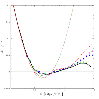
Figure 2: The fractional difference between the nonlinear mass power spectra at $z=0.5$ for $\alpha(k_{0}=0.2h/{\rm Mpc})=0.04$ and $\alpha(k_{0}=0.2h/{\rm Mpc})=-0.04$, $[P(k,\alpha=+0.04)-P(k,\alpha=-0.04)]/\bar{P}(k)$, where $\bar{P}(k)=[P(k,\alpha=+0.04)+P(k,\alpha=-0.04)]/2$. All other parameters are fixed at their fiducial values. The dotted line is linear theory The solid line is from an $L=320h^{-1}{\rm Mpc}$, $N=256^{3}$ simulation. The open squares, filled squares, and triangles are from $L=160h^{-1}{\rm Mpc}$ simulations with $N=512^{3}$, $N=256^{3}$, and $N=128^{3}$, respectively. Note that the triangle at the highest k is well beyond the resolution limit of the simulations. The dashed line is from halofit.

To be sure that our results have numerically converged, we compare simulations with box size $L=320h^{-1}{\rm Mpc}$ and $N=256^{3}$ particles (our mesh for the force calculation is always a factor of 2 finer than the mean particle spacing) to simulations with $L=160h^{-1}{\rm Mpc}$ and $N=128^{3}$ (the same resolution as the bigger box), $N=256^{3}$, or $N=512^{3}$. In Fig. 2 we note first that the difference between the two box sizes is probably insignificant (solid line vs. triangles). The $L=160h^{-1}{\rm Mpc}$, $N=256^{3}$ box has sufficient resolution to compute derivatives accurately out to $k=10h/{\rm Mpc}$ (open vs. closed squares). Turning to the comparison between halofit and the simulations, we see that the fitting formula does well if one is not interested in the fine details of the nonlinear power; however, a Fisher matrix constraint that actually relies on the value of the derivative at $k\sim 0.2h/{\rm Mpc}$ (rather than just the fact that it is close to zero) would be inaccurate.

Figure 3: The fractional difference between the convergence power spectra for $\alpha(k_{0}=0.2h/{\rm Mpc})=0.04$ and $\alpha(k_{0}=0.2h/{\rm Mpc})=-0.04$, $[P_{\kappa}(l,\alpha=+0.04)-P_{\kappa}(l,\alpha=-0.04)]/\bar{P_{\kappa}}(l)$, where $\bar{P_{\kappa}}(l)=[P_{\kappa}(l,\alpha=+0.04)+P_{\kappa}(l,\alpha=-0.04)]/2$. All other parameters are fixed at their fiducial values. The solid line is from an $L=320h^{-1}{\rm Mpc}$, $N=256^{3}$ simulation. The open squares and filled squares are from $L=160h^{-1}{\rm Mpc}$ simulations with $N=512^{3}$ and $N=256^{3}$ respectively. The dashed line is from halofit.

We show in 3 how the differences in the sc halofit and n-body mass power spectra are transferred to the convergence power spectra.

For the combination of CMB and lensing we use the pivot point $k_{0}=0.05h/{\rm Mpc}$. Figure 4 shows the comparison between the simulations and halofit for this $k_{0}$.

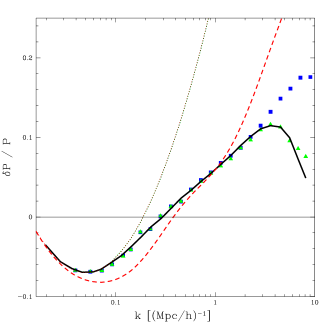
Figure 4: The fractional difference between the nonlinear mass power spectra at $z=0.5$ for $\alpha(k_{0}=0.05h/{\rm Mpc})=0.04$ and $\alpha(k_{0}=0.05h/{\rm Mpc})=-0.04$. The dotted line is linear theory. The solid line is from an $L=320{\rm Mpc}/h$, $N=256^{3}$ simulation. The squares and triangles are from $L=160{\rm Mpc}/h$ simulations with $N=256^{3}$ and $N=128^{3}$, respectively. The dashed line is from halofit.

The result is similar to the $k_{0}=0.2h/{\rm Mpc}$ case, i.e., the basic trend is correct but the details are not completely correct. The same could be said of the results for variation in $n$, shown in Fig. 5.

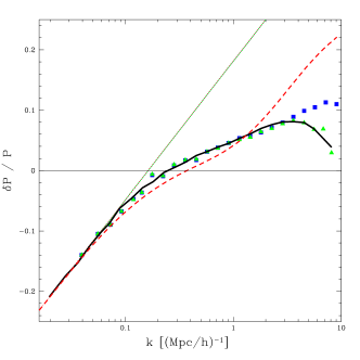
Figure 5: The fractional difference between the nonlinear mass power spectra at $z=0.5$ for $n=1.0$ and $n=0.9$. The dotted line is linear theory. The solid line is from an $L=320{\rm Mpc}/h$, $N=256^{3}$ simulation. The squares and triangles are from $L=160{\rm Mpc}/h$ simulations with $N=256^{3}$ and $N=128^{3}$, respectively. The dashed line is from halofit.

The comparisons for variations in $\sigma_{8}$, $\Omega_{\Lambda}$, and $\Omega_{m}h^{2}$ are shown in Figures 6, 7, and 8, respectively. Generally the agreement for these cases seems better (i.e., very good). For $k\lesssim 2h/{\rm Mpc}$ the error in the prediction of the derivatives by the fitting formula is not large, even as a fraction of the values of the derivatives.

Note that our comparison of halofit to the simulations has been restricted to the fractional change between models, and implies nothing about the accuracy of halofit for predicting the absolute power spectrum, which is necessary when interpreting data. Our simulations are not suited to predicting the absolute power – on large scales they have big statistical fluctuations due to limited box size, while on small scales the power is suppressed by the limited PM resolution. Both of these effects cancel neatly in the fractional derivatives that we show, and for our Fisher matrix calculation this is sufficient.

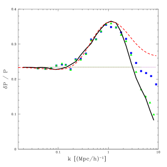
Figure 6: The fractional difference between the nonlinear mass power spectra at $z=0.5$ for $\sigma_{8}=0.9$ and $\sigma_{8}=0.8$. See Fig. 5 for line meanings.

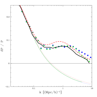
Figure 7: The fractional difference between the nonlinear mass power spectra at $z=0.5$ for $\Omega_{\Lambda}=0.78$ and $\Omega_{\Lambda}=0.7$. See Fig. 5 for line meanings.

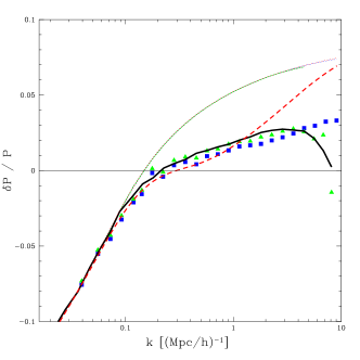
Figure 8: The fractional difference between the nonlinear mass power spectra at $z=0.5$ for $\Omega_{m}h^{2}=0.149$ and $\Omega_{m}h^{2}=0.129$. See Fig. 5 for line meanings.

IV Parameter forecasts

IV.1 Fisher-matrix analysis

The uncertainty in the observed weak lensing spectrum is given by: Kaiser (1992, 1998)

$$\Delta P_{\kappa}(\ell)=\sqrt{\frac{2}{(2\ell+1)f_{sky}}}\left(P_{\kappa}(\ell)+{\left<\gamma_{int}{}^{2}\right>\over\bar{n}}\right)\,,$$ (9)

where $f_{sky}=\Theta^{2}\pi/129600$ is the fraction of the sky covered by a survey of dimension $\Theta$ in degrees, $\left<\gamma_{int}^{2}\right>^{1/2}\approx 0.4$ is the intrinsic ellipticity of galaxies. We assume for a Reference Survey a sky coverage of $f_{sky}=0.01$ and an average galaxy number density of $\bar{n}\approx 6.6\times 10^{8}{\rm sr}^{-1}$; we will also investigate the effects of varying both of these parameters.

The Fisher-matrix formalism for cosmological parameter forecast has been proven in previous studies to be a powerful tool for estimating the statistical errors achievable by experiments Eisenstein et al. (1999); Zaldarriaga et al. (1997); Bond et al. (1997); Hu and Tegmark (1999); Huterer (2002). If the convergence field is Gaussian, and the noise is a combination of Gaussian shape and instrument noise with no intrinsic correlations, the Fisher matrix is given by:

$$F_{\alpha\beta}={\sum_{\ell=\ell_{\rm min}}^{\ell_{\rm max}}{\frac{(\ell+1/2)f_{sky}}{(P_{\kappa}+\left<\gamma_{\rm int}^{2}\right>/\bar{n})^{2}}{\frac{\partial P_{\kappa}}{\partial p^{\alpha}}}}{\frac{\partial P_{\kappa}}{\partial p^{\beta}}}};$$ (10)

we have used $\ell_{\rm max}=3000$ since on smaller scales, the assumption of a Gaussian shear field underlying Eq. (10) and the halofit approximation to the nonlinear power spectrum may not be valid. (Note that the shear field is a projection through many nearly independent structures, so by the Central Limit Theorem it can be well-described by Gaussian statistics even when the density perturbations are not Gaussian. Even with the Central Limit Theorem, deviations of the shear field from Gaussian statistics become large at the 1–2 arcmin scale Jain et al. (2000); Cooray and Hu (2001).) On small scales, there is cosmological information in the small-scale non-Gaussianity (e.g. skewness) of the lensing field Bernardeau et al. (1997), but we do not investigate this here. For the minimum $\ell$, we take the fundamental mode approximation:

$$\ell_{\rm min}\approx\frac{360\rm~{}deg}{\Theta}=\sqrt{\pi\over f_{sky}},$$ (11)

i.e. we consider only lensing modes for which at least one wavelength can fit inside the survey area. The survey contains some information on larger angular scales, and for this reason the approximation Eq. (11) might be considered conservative. However, it should also be noted that some of the planned surveys will scan disconnected regions of the sky in order to provide additional systematic error checks, in which case the effective $\ell_{\rm min}$ is increased.

The statistical error on a given parameter $p_{\alpha}$ is then given by:

$$\sigma^{2}(p_{\alpha})\approx[({\bf F}+\Pi)^{-1}]_{\alpha\alpha},$$ (12)

where $\Pi$ is the prior curvature matrix. We only impose priors on the source redshift and on the calibration parameters (see §II.3). For the Reference Survey, we take priors of $\sigma(\zeta_{s})=\sigma(\zeta_{r})=0.02$ on the calibration parameters Hirata and Seljak (2003) and $\sigma(z_{p})=0.05$ on the source redshifts. Since the primary CMB anisotropies are generated at much larger comoving distance than the density fluctuations that give rise to weak lensing, it is a good approximation to take them to be independent; in this case, we can add the Fisher matrices from lensing and CMB to yield combined constraints on cosmological parameters. This combination leads to significant improvements in parameter estimation as we show in Fig. 9.

Figure 9: Improvements of the CMB parameter estimation with weak lensing. The effect of increasing $f_{sky}$ is displayed here.

IV.2 Adding tomography

Tomography has been shown to improve significantly the measurements of cosmological parameters Hu (1999, 2002). We explore the impact on parameter estimation from tomographic separation of the source galaxies into two redshift bins; see Eq. (5). The Fisher formalism is generalized here using:

$$F_{\alpha\beta}=\sum_{\ell_{\rm min}}^{\ell_{\rm max}}(\ell+1/2)f_{\rm sky}{\rm Tr}\left({\bf C}_{\ell}^{-1}{\partial{\bf P}_{\ell}\over\partial p^{\alpha}}{\bf C}_{\ell}^{-1}{\partial{\bf P}_{\ell}\over\partial p^{\beta}}\right),$$ (13)

where ${\bf C}_{\ell}$ is the covariance matrix of the multipole moments of the observables ${C}^{\kappa\kappa^{\prime}}_{\ell}=P_{\ell}^{\kappa\kappa^{\prime}}+N_{\ell}^{\kappa\kappa^{\prime}}$ with $N_{\ell}^{\kappa\kappa^{\prime}}$ the power spectrum of the noise in the measurement. These read

$${P}^{\kappa\kappa^{\prime}}_{\ell}=\left(\begin{array}[]{cc}P_{\ell}^{AA}&P_{\ell}^{AB}\\ P_{\ell}^{AB}&P_{\ell}^{BB}\end{array}\right),$$ (14)

and

$${N}^{\kappa\kappa^{\prime}}_{\ell}=\left(\begin{array}[]{cc}{\left<\gamma_{\rm int}^{2}\right>/\bar{n}_{A}}&0\\ 0&{\left<\gamma_{\rm int}^{2}\right>/\bar{n}_{B}}\end{array}\right).$$ (15)

The convergence power spectra for the two bins and their cross correlation are shown in Fig. 10.

Figure 10: Convergence power spectra for bin A, bin B and their cross correlation. $\alpha_{s}=-0.04$ and $k_{0}=0.05h/Mpc$.

IV.3 Results

Table 1: A comparative table for parameter estimation errors from our Reference Survey with $f_{sky}=0.01$ and $\bar{n}=6.6\times 10^{8}{\rm sr}^{-1}$. The first row (C) are uncertainties from the CMB=WMAP(1yr)+CBI+ACBAR alone. The following rows show combined errors for CMB plus weak lensing in the Reference Survey (CW), and CMB plus weak lensing with tomography (CT). The lower-case suffixes a,b,c indicate the priors used: (a) prior of $0.1$ on $\zeta_{s}$ and $\zeta_{r}$ (if applicable), and $0.05$ on $z_{p}$; (b) prior of $0.02$ on $\zeta_{s}$ and $\zeta_{r}$) and $0.05$ on $z_{p}$; and (c) prior of $10^{-4}$ on $\zeta_{s}$, $\zeta_{r}$, and $z_{p}$ (i.e. effectively perfect knowledge of calibration and source redshift is assumed). For the rows labeled with [S], the $N$-body simulation was used to provide the matter power spectra instead of using halofit. Note that the simulated and halofit results are very similar.

	$\sigma(\Omega_{m}h^{2})$	$\sigma(\Omega_{b}h^{2})$	$\sigma(\Omega_{\Lambda})$	$\sigma(\sigma_{8})$	$\sigma(n_{s})$	$\sigma(\alpha_{s})$	$\sigma(\tau)$	$\sigma(T/S)$	$\sigma(z_{p})$	$\sigma(\zeta_{s})$	$\sigma(\zeta_{r})$
C	0.013	0.0012	0.054	0.083	0.036	0.039	0.035	0.154	-	-	-
CWa	0.0036	0.0010	0.0191	0.024	0.021	0.017	0.033	0.143	0.042	0.092	0.099
CWb	0.0030	0.0010	0.0167	0.023	0.021	0.017	0.033	0.143	0.041	0.020	0.020
CWc	0.0027	0.0010	0.0145	0.022	0.021	0.017	0.033	0.142	0.0001	0.0001	0.0001
CTa	0.0034	0.0010	0.0170	0.021	0.020	0.016	0.031	0.140	0.029	0.075	0.024
CTb	0.0029	0.0009	0.0159	0.017	0.019	0.015	0.030	0.138	0.027	0.020	0.015
CTc	0.0027	0.0008	0.0069	0.010	0.016	0.013	0.023	0.130	0.0001	0.0001	0.0001
CWb[S]	0.0032	0.0010	0.0169	0.024	0.022	0.019	0.034	0.142	0.045	0.020	0.020
CWc[S]	0.0027	0.0010	0.0151	0.023	0.022	0.019	0.034	0.142	0.0001	0.0001	0.0001
CTb[S]	0.0030	0.0009	0.0147	0.017	0.015	0.014	0.030	0.125	0.024	0.020	0.014
CTc[S]	0.0025	0.0008	0.0069	0.010	0.014	0.013	0.022	0.123	0.0001	0.0001	0.0001

We generated the convergence power spectra using a weak lensing code that includes the formalism and features described in §II. We derived parameter uncertainties for weak lensing with and without tomography and then combine these errors with the CMB analysis. We used the CMB parameter estimation uncertainties of Ref. Seljak et al. (2003) (the correlation matrix was provided by the authors). As described in their paper, the authors have used a standard Monte Carlo Markov Chain using the WMAP+CBI+ACBAR data (we will refer to these as “CMB”). In Table 1, we show the values for the uncertainties from CMB alone and then from a combination of CMB with weak lensing with and without tomography for our reference survey ($f_{sky}=0.01$ and $\bar{n}=6.6\times 10^{8}{\rm sr}^{-1}$.)

We summarize in Table 2 and Table 3 the results respectively for increasing values of $f_{sky}$ and $\bar{n}$. We show the full correlation matrices for combined CMB and weak lensing observations with and without tomography in Table 4. In Table 5, we have fixed the calibration parameters and the characteristic redshift of the source galaxies. This significantly improves the precision of cosmological parameter estimates; we can see from the correlation matrix (Table 4) that most of this improvement comes from the fixing the source redshift. As can be seen from Table 2, very stringent cosmological constraints can in principle be obtained for surveys covering thousands of square degrees; however, equally stringent controls over systematic errors would be required. An additional caveat is the possibility of errors in the parameter constraints at very high $f_{sky}$ (i.e. the bottom row of Tables 2 and 5), since there the Fisher matrix is poorly conditioned and inaccuracies in our computation of the derivatives $\partial P_{\kappa}(\ell)/\partial p^{\alpha}$ are thus magnified.

It is worth noting from the correlation matrix (Table 4) that the calibration parameters are not degenerate with any of the cosmological parameters considered. This lack of degeneracy is good news because it means that weak lensing surveys can be used for precision cosmology even if the absolute shear calibration cannot be determined with high accuracy. Note that the current data analysis methods for lensing are estimated to have amplitude calibration correct at roughly the $\sim 5$% level; the power calibration is twice this, or $\pm 0.1$ Hirata and Seljak (2003). If we impose only this $\pm 0.1$ prior on $\zeta_{s}$ and $\zeta_{r}$ (and retain the $\pm 0.05$ prior on $z_{p}$), we see that the uncertainties on cosmological parameters are essentially unchanged (Table 1). With this weaker prior, the correlation of the calibration parameters with $z_{p}$, $\sigma_{8}$, and $\Omega_{\Lambda}$ becomes larger ($|\rho|>0.5$), and with even weaker priors the uncertainties in these parameters are degraded.

Table 2: Parameter estimation errors for weak lensing combined with CMB: $f_{sky}$ is varied from $10^{-5}$ to 1.0. and $\bar{n}=6.6\times 10^{8}{\rm sr}^{-1}$. We use priors of 0.02 on $\zeta_{s}$ and $\zeta_{r}$ and 0.05 on $z_{p}$. Tomography is added in the second part of the table.

$f_{sky}$	$\sigma(\Omega_{m}h^{2})$	$\sigma(\Omega_{b}h^{2})$	$\sigma(\Omega_{\Lambda})$	$\sigma(\sigma_{8})$	$\sigma(n_{s})$	$\sigma(\alpha_{s})$	$\sigma(\tau)$	$\sigma(T/S)$	$\sigma(z_{p})$	$\sigma(\zeta_{s})$	$\sigma(\zeta_{r})$
0.00001	0.0052	0.0011	0.0266	0.035	0.034	0.038	0.035	0.148	0.050	0.020	0.020
0.00010	0.0037	0.0011	0.0216	0.026	0.032	0.035	0.035	0.147	0.050	0.020	0.020
0.00100	0.0033	0.0010	0.0182	0.025	0.025	0.025	0.034	0.145	0.048	0.020	0.020
0.01000	0.0030	0.0010	0.0167	0.023	0.021	0.017	0.033	0.143	0.041	0.020	0.020
0.10000	0.0028	0.0009	0.0160	0.018	0.019	0.015	0.031	0.138	0.026	0.020	0.020
1.00000	0.0022	0.0008	0.0132	0.015	0.016	0.012	0.026	0.119	0.018	0.019	0.020
0.00001	0.0051	0.0011	0.0264	0.034	0.034	0.038	0.035	0.148	0.049	0.020	0.020
0.00010	0.0037	0.0011	0.0215	0.025	0.031	0.035	0.034	0.147	0.047	0.020	0.020
0.00100	0.0032	0.0010	0.0180	0.020	0.024	0.023	0.032	0.143	0.037	0.020	0.019
0.01000	0.0029	0.0009	0.0159	0.017	0.019	0.015	0.030	0.138	0.027	0.020	0.015
0.10000	0.0026	0.0008	0.0122	0.014	0.016	0.012	0.026	0.122	0.019	0.018	0.008
1.00000	0.0019	0.0006	0.0067	0.009	0.010	0.007	0.020	0.091	0.011	0.014	0.003

Table 3: Parameter estimation errors for weak lensing combined with CMB: $\bar{n}$ is varied from $\bar{n}=5.0\times 10^{6}{\rm sr}^{-1}$ to $\bar{n}=1.0\times 10^{9}{\rm sr}^{-1}$; $f_{sky}=0.01$. With a prior of 0.02 on $\zeta_{r}$ and $\zeta_{s}$ and 0.05 on $z_{p}$. Tomography is added in the second part of the table.

$\bar{n}$	$\sigma(\Omega_{m}h^{2})$	$\sigma(\Omega_{b}h^{2})$	$\sigma(\Omega_{\Lambda})$	$\sigma(\sigma_{8})$	$\sigma(n_{s})$	$\sigma(\alpha_{s})$	$\sigma(\tau)$	$\sigma(T/S)$	$\sigma(z_{p})$	$\sigma(\zeta_{s})$	$\sigma(\zeta_{r})$
$5.0\times 10^{6}$	0.0045	0.0011	0.0239	0.032	0.034	0.038	0.035	0.149	0.050	0.020	0.020
$1.0\times 10^{7}$	0.0035	0.0011	0.0194	0.028	0.030	0.033	0.035	0.147	0.049	0.020	0.020
$5.0\times 10^{7}$	0.0032	0.0010	0.0173	0.024	0.023	0.022	0.034	0.145	0.046	0.020	0.020
$1.0\times 10^{8}$	0.0032	0.0010	0.0170	0.024	0.022	0.020	0.034	0.144	0.044	0.020	0.020
$5.0\times 10^{8}$	0.0031	0.0010	0.0167	0.023	0.021	0.017	0.033	0.143	0.041	0.020	0.020
$1.0\times 10^{9}$	0.0030	0.0010	0.0166	0.022	0.021	0.017	0.033	0.143	0.040	0.020	0.020
$5.0\times 10^{6}$	0.0048	0.0011	0.0247	0.033	0.034	0.038	0.035	0.149	0.050	0.020	0.020
$1.0\times 10^{7}$	0.0036	0.0011	0.0197	0.028	0.030	0.034	0.035	0.147	0.049	0.020	0.020
$5.0\times 10^{7}$	0.0032	0.0010	0.0173	0.021	0.022	0.021	0.033	0.143	0.040	0.020	0.019
$1.0\times 10^{8}$	0.0031	0.0010	0.0168	0.019	0.021	0.019	0.032	0.142	0.035	0.020	0.018
$5.0\times 10^{8}$	0.0029	0.0009	0.0159	0.017	0.019	0.016	0.031	0.138	0.027	0.020	0.015
$1.0\times 10^{9}$	0.0028	0.0009	0.0148	0.015	0.018	0.014	0.030	0.133	0.023	0.019	0.009

Table 4: Correlation matrix for parameter estimation errors for weak lensing combined with CMB. $\bar{n}=6.6e8$ and $f_{sky}=0.01$. With a prior of 0.02 on $\zeta_{r}$ and $\zeta_{s}$, and 0.05 on $z_{p}$. The above-diagonal elements correspond to a survey without tomography; the below-diagonal elements correspond to a survey with tomography.

	$\Omega_{m}h^{2}$	$\Omega_{\Lambda}$	$\sigma_{8}$	$n_{s}$	$\alpha_{s}$	$z_{p}$	$\zeta_{s}$	$\zeta_{r}$	$\Omega_{b}h^{2}$	$\tau$	$T/S$
$\Omega_{m}h^{2}$	1	-0.325	-0.020	0.135	-0.266	-0.430	-0.137	0.017	0.378	-0.533	0.313
$\Omega_{\Lambda}$	-0.375	1	0.754	0.667	-0.583	0.464	0.122	-0.018	0.558	0.728	0.393
$\sigma_{8}$	-0.230	0.877	1	0.632	-0.679	-0.160	-0.091	0.008	0.541	0.757	0.375
$n_{s}$	0.072	0.651	0.620	1	-0.774	0.104	0.022	-0.002	0.788	0.393	0.794
$\alpha_{s}$	-0.228	-0.550	-0.626	-0.770	1	-0.076	0.026	0.005	-0.716	-0.433	-0.752
$z_{p}$	-0.386	0.818	0.570	0.444	-0.455	1	-0.052	0.020	0.092	0.126	0.096
$\zeta_{s}$	-0.156	0.078	-0.217	-0.028	0.106	-0.045	1	0.002	0.014	0.004	0.013
$\zeta_{r}$	0.086	0.158	0.386	0.221	-0.204	-0.243	0.083	1	-0.003	-0.005	-0.004
$\Omega_{b}h^{2}$	0.349	0.527	0.516	0.762	-0.698	0.371	-0.033	0.185	1	0.372	0.673
$\tau$	-0.680	0.726	0.732	0.329	-0.321	0.572	-0.049	0.176	0.311	1	0.136
$T/S$	0.294	0.355	0.357	0.786	-0.756	0.266	-0.028	0.133	0.650	0.073	1

Table 5: Parameter estimation errors for weak lensing combined with CMB: Here we have fixed $\zeta_{r}$, $\zeta_{s}$ and $z_{p}$ by imposing priors of width $10^{-4}$ on these parameters; $f_{sky}$ is varied from $10^{-5}$ to 1.0; $\bar{n}=6.6\times 10^{8}{\rm sr}^{-1}$. Tomography is added in second part of the table.

$f_{sky}$	$\sigma(\Omega_{m}h^{2})$	$\sigma(\Omega_{b}h^{2})$	$\sigma(\Omega_{\Lambda})$	$\sigma(\sigma_{8})$	$\sigma(n_{s})$	$\sigma(\alpha_{s})$	$\sigma(\tau)$	$\sigma(T/S)$	$\sigma(z_{p})$	$\sigma(\zeta_{s})$	$\sigma(\zeta_{r})$
0.00001	0.0050	0.0011	0.0260	0.034	0.034	0.038	0.035	0.148	0.0001	0.0001	0.0001
0.00010	0.0034	0.0011	0.0206	0.025	0.032	0.035	0.035	0.147	0.0001	0.0001	0.0001
0.00100	0.0029	0.0010	0.0169	0.023	0.025	0.025	0.034	0.145	0.0001	0.0001	0.0001
0.01000	0.0027	0.0010	0.0145	0.022	0.021	0.017	0.033	0.142	0.0001	0.0001	0.0001
0.10000	0.0026	0.0009	0.0105	0.016	0.017	0.013	0.027	0.132	0.0001	0.0001	0.0001
1.00000	0.0022	0.0007	0.0044	0.007	0.011	0.008	0.019	0.104	0.0001	0.0001	0.0001
0.00001	0.0049	0.0011	0.0258	0.033	0.034	0.038	0.035	0.148	0.0001	0.0001	0.0001
0.00010	0.0033	0.0011	0.0204	0.024	0.031	0.035	0.034	0.147	0.0001	0.0001	0.0001
0.00100	0.0029	0.0010	0.0146	0.019	0.023	0.022	0.031	0.140	0.0001	0.0001	0.0001
0.01000	0.0027	0.0008	0.0069	0.010	0.016	0.013	0.023	0.130	0.0001	0.0001	0.0001
0.10000	0.0024	0.0007	0.0024	0.003	0.012	0.008	0.019	0.112	0.0001	0.0001	0.0001
1.00000	0.0019	0.0006	0.0008	0.001	0.007	0.004	0.017	0.085	0.0001	0.0001	0.0001

V Discussion

In accord with previous studies, we find that when weak lensing surveys are combined with the CMB results, the uncertainties on the cosmological parameters are reduced. The improvement can be up to an order of magnitude, depending on the size and depth of the survey (see Table 2 and Table 3). It is well known that weak lensing and CMB have different types of degeneracies in their parameters which are nicely broken when combined together. In particular, weak lensing does not suffer from the well-known angular diameter distance degeneracy; and it probes smaller comoving scales than the CMB, which means that it has a different degeneracy direction in the $(n_{s},\alpha_{s})$ plane. The improvements from including weak lensing are especially notable for $\sigma_{8}$, $\Omega_{m}h^{2}$ and $\Omega_{\Lambda}$.

Motivated by recent discussion concerning the running of the primordial power spectrum $\alpha_{s}$, we include it as a parameter in the weak lensing analysis. We find that for small surveys, modest improvement is obtained for $n_{s}$ and $\alpha_{s}$. Our Reference Survey can reduce $\sigma(n_{s})$ and $\sigma(\alpha_{s})$ by roughly a factor of two. For surveys within the near future (see Refs. in §I), weak lensing can be used to provide complementary constraints to detect a possible running spectral index, but may not be able to verify the results obtained by combined CMB+Lyman-$\alpha$ forest analysis, which should give another factor of 2-4 lower $\sigma(\alpha_{s})$. A detailed comparative study of the constraints from the two probes is left for future work. We find that tomography improves in particular the uncertainty on $\sigma_{8}$ and $\Omega_{\Lambda}$. For the Reference Experiment, we do not find large improvements in the other parameters from tomography except for the most ambitious surveys. This can be attributed to the strong parameter degeneracies present even when tomography is used (see Table 4), most notably the degeneracy between $\Omega_{\Lambda}$ and $z_{p}$. If the source redshift distribution is known accurately from a spectroscopic redshift survey, then this degeneracy is lifted, and tomography becomes a powerful tool for measuring cosmological parameters, including $\Omega_{\Lambda}$, $n_{s}$ and $\alpha_{s}$ (see Table 5). A comparison of Tables 2 and 5 shows that the parameter constraints from tomography are more sensitive to the systematics parameters than the constraints without tomography, hence the benefits of tomography can only be fully realized if systematic errors are tightly controlled.

We expanded the usual weak lensing parameter space to include two calibration parameters in addition to the characteristic redshift of source galaxies. We hope that the present analysis will encourage weak lensing observers to expand their likelihood analyses to include a parameterization of systematic errors. It is already common practice to report results marginalized over the characteristic source redshift Contaldi et al. (2003); Hoekstra et al. (2002a, b) or to treat it as a systematic to be added in quadrature to statistical errors Jarvis et al. (2003). Ultimately it would be desirable to include not just the calibration factors and characteristic source redshift but also the full redshift distribution of sources, intrinsic alignments, etc. Additional data (such as spectroscopic redshifts) and detailed analysis and simulations may be required in order to constrain some of these parameters. However, in some cases it is possible to obtain information about the systematics parameters from the data itself. For example, the nonlinear portion of the convergence power spectrum provides joint constraints on the shear calibration biases $\zeta_{s}$ and $\zeta_{r}$ and the cosmological parameters.

We have shown, at least at the level of our Reference Survey, that halofit provides a sufficiently good fit to $N$-body simulations for use in parameter forecasting studies. The largest discrepancy is $25$% in the error on $n_{s}$ when tomography is included, but most of the error estimates agree to better than 10%. Note that this does not imply that the nonlinear mapping is sufficiently accurate for analysis of Reference Survey data, since the best-fit values of cosmological parameters can be significantly affected by small errors in theoretical predictions even if the fractional change in the Fisher matrix is small.

In summary, we have shown that weak lensing, supplemented with the one-year WMAP data, has the potential to very precisely measure the running of the scalar spectral index. This would provide a third measurement of $\alpha_{s}$ in addition to those using the Lyman-$\alpha$ forest and/or galaxy power spectrum, and the precision measurement of the high-$\ell$ CMB power spectrum expected from Planck. Weak lensing observations are currently progressing rapidly and the data required to significantly improve WMAP constraints on $\alpha_{s}$ should be available in the foreseeable future. By providing an additional and mostly independent measurement of the value of $\alpha_{s}$ (and more generally the scalar power spectrum) obtained by these other methods, weak lensing will help us to understand the spectrum of primordial scalar fluctuations in the universe and thus provide valuable information on the mechanism of their generation.