[astro-ph/0308427] Chapter 1 Performance of the Pierre Auger Fluorescence Detector and Analysis of Well Reconstructed Events

Abstract

The Pierre Auger Observatory is designed to elucidate the origin and nature of Ultra High Energy Cosmic Rays using a hybrid detection technique. A first run of data taking with a prototype version of both detectors (the so called Engineering Array) took place in 2001-2002, allowing the Collaboration to evaluate the performance of the two detector systems and to approach an analysis strategy. In this contribution, after a brief description of the system, we will report some results on the behavior of the Fluorescence Detector (FD) Prototype. Performance studies, such as measurements of noise, sensitivity and duty cycle, will be presented. We will illustrate a preliminary analysis of selected air showers. This analysis is performed using exclusively the information from the FD, and includes reconstruction of the shower geometry and of the longitudinal profile.

Introduction

The Pierre Auger Cosmic Ray observatory will be the largest cosmic ray detector ever built. Two sites of approximately 3000 km² , one in each hemisphere, will be instrumented with a surface detector and a set of fluorescence detectors. Two fluorescence telescope units were operated from December 2001 to March 2002 in conjunction with 32 surface detectors, the so-called Engineering Array. This phase of the project was aimed at proving the validity of the design and probing the potential of the system. In the following we will show an analysis of the performance of the FD during this run and demonstrate, by investigating selected events, the ability to reconstruct geometry and the longitudinal profile of Extensive Air Showers.

System Overview

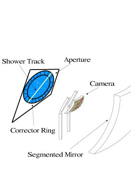
Figure LABEL:009385-1:fig:tel shows a schematic view of a fluorescence telescope unit. An array of 20 $\times$ 22 hexagonal photomultiplier tubes (the camera) is mounted on a quasi-spherical support located at the focal surface of a segmented mirror [1]. Each PMT overlooks a region of the sky of 1.5 deg in diameter. The telescope aperture has a diameter of 2.20 m and features an optical filter (MUG-6) to select photons in the range 300-400 nm. A Schmidt corrector ring allows the collection area to be doubled without increasing the effects of optical aberrations. The Schmidt geometry results in a 30 ${}^{\circ}\times$ 30^∘ field of view for each telescope unit. The final design envisages four eyes each of six telescopes.

Refer to caption — Fig. 1.: Schematic view of a Fluorescence Telescope unit

The current signal coming
from each phototube is sampled at 10 MHz with 12 bit resolution and 15 bit dynamic range. The First Level Trigger system performs a boxcar running sum of ten samples. When the sum exceeds a threshold, the trigger is fired. This threshold is determined by the trigger rate itself, and is regulated to keep it close to 100 Hz. Every microsecond, the camera is scanned for patterns of fired pixels that are consistent with a track induced by the fluorescence light from a shower. This is the Second Level Trigger, that in the Engineering Array run had a rate of 0.3 Hz. It is dominated by muons hitting the camera directly and random noise. These components, as well as lightning, are then filtered by the software Third Level Trigger, yielding a rate of 8 $\times$ 10^-4 Hz (one event every 20 mn) per telescope.

System Performance

We will briefly report on some measured parameters that give an indication of the performance of the optics and of the electronics. The size of the light spot on the focal surface gives an indication on the quality of the optics and the alignment of the mirrors. This has been measured by placing a white screen on the camera and then using a CCD device to capture images from bright stars, which can effectively be considered as point sources. Measurements taken for different star positions (therefore different light incidence angles) show that 90% of the light is collected within a circle of 1.8 cm (0.65 deg) diameter. The reflectivity of each mirror segment was measured to be above 90%.
The most important parameter of the front-end electronics is the noise level. The design requires a system contribution of less than 10% of total noise, which is dominated by the light background from the night sky. The contribution of the electronics has been measured by comparing the fluctuation of the baseline of the sampled signal in dark conditions, $\sigma_{elec}$ , with that determined when the detector is exposed to the night sky, $\sigma_{sky+elec}$ . The ratio ${\sigma_{sky+elec}}/{\sigma_{sky}}$ , averaged over all the pixels, gives a value of 1.06 . The noise contribution of the sky alone is here calculated as $\sigma_{sky}=\sqrt{\sigma^{2}_{sky+elec}-\sigma^{2}_{elec}}$ .

The sensitivity of the system to distant showers has been estimated using a portable laser system. This frequency-tripled YAG laser features adjustable energy, measured by means of a radiometer applied to a portion of the beam. The laserscope was brought to a distance of 26 km, and the energy lowered in steps while the drop in FD trigger efficiency was being watched. Although the measurements should be extended and improved, they indicate a threshold around 10 EeV at 26 km. The Fluorescence Detector prototype was run smoothly during the period December 2001 - March 2002. During this time it has collected over 1000 shower candidates and several hundred laser shots for detector studies. It was operated from 30 mn after astronomical dusk to 30 mn before dawn, in periods when the fraction of illuminated moon was below 50%. The duty cycle was 11%, close to the figure foreseen for normal operation. In the next section we will present the preliminary technique used to reconstruct the longitudinal profile of a selected sample of showers.

Reconstruction

The methods to reconstruct the shower geometry with a monocular FD alone are described in another contribution [3], where the detector geometrical resolution is presented. In the following we will outline the procedure used to reconstruct the longitudinal profile and primary energy from Engineering Array data.
The received light flux $S(X)$ originating in a layer between $X$ and $X+\delta X$ , where $X$ is the atmospheric depth in $g/cm^{2}$ , may be approximated by:

{}S(X)=L(X)\frac{A}{4\pi r^{2}}~{}c~{}\delta t\cdot\epsilon\cdot{\mathcal{T}}(r)

(1)

where $L(X)$ is the fluorescence light isotropically emitted at the source (equal to the product of the yield at height $h$ , $F_{y}(h)$ , and the shower size $n_{e}(X)$ ), $A$ is the collection area, $r$ the observation distance, $\delta t$ is the time the shower takes to travel from $X$ to $X+\delta X$ when viewed from the detector ( $\delta t$ depends solely on the geometry), $\epsilon$ is the collection efficiency and $\mathcal{T}(r)$ factorizes the transmission of the atmosphere. The calibration chain [4] gives the signal in units of 370 nm equivalent photons at the aperture. Therefore, to reconstruct the incident flux as a function of time, $S(t)$ , it is sufficient to collect the calibrated signal from all pixels within an angle $\zeta$ from the shower track. $\zeta$ is chosen so as to maximize the signal to noise ratio. The next step is to evaluate $L(X)$ from $S(t)$ . This is done by unfolding the effect of the atmosphere transmission using, in this preliminary analysis, a standard atmosphere model to deal with Rayleigh and aerosol components. The fluorescence yield $F_{y}(h)$ must then be estimated in order to obtain $N_{e}(X)$ . The measured fluorescence yield from [2] is used. The contribution of direct and scattered Cerenkov light is then subtracted with an iterative procedure. The electromagnetic energy is calculated as: $E_{em}=\frac{E_{c}}{X_{r}}\int n_{e}(X)dX$ where $n_{e}(X)$ is the number of electrons at depth X[ $g\cdot{cm^{-2}}$ ], $E_{c}$ is the critical energy of electrons in air and $X_{r}$ their radiation length.
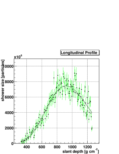
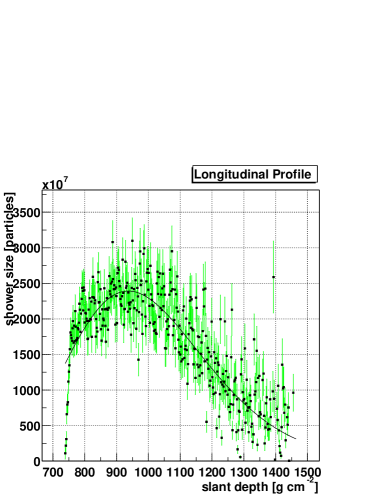
We selected a sample of about 50 events recorded during the Engineering Array run to exercise the presented reconstruction method. Examples are shown if Figure LABEL:009385-1:fig:rec

Conclusions

The Engineering Array run has proved that the Fluorescence Detector prototype meets design specifications and performs appropriately. It was possible to reconstruct the longitudinal profiles of several showers.

References

1. Auger Collaboration , “Technical Design Report”, www.auger.org

2. Kakimoto F. et al, 1996, Nucl. Instrum. Meth. A372, 527

3. Privitera, P. , these Proceedings

4. Roberts, M. , these Proceedings