A spatially resolved limb flare on Algol B observed with XMM-Newton

We report XMM-Newton observations of the eclipsing binary Algol A (B8V) and B (K2III). The XMM-Newton data cover the phase interval 0.35 – 0.58, i.e., specifically the time of optical secondary minimum, when the X-ray dark B-type star occults a major fraction of the X-ray bright K-type star. During the eclipse a flare was observed with complete light curve coverage. The decay part of the flare can be well described with an exponential decay law allowing a rectification of the light curve and a reconstruction of the flaring plasma region. The flare occurred near the limb of Algol B at a height of about 0.1 R_⋆ with plasma densities of a few times 10¹¹ cm^-3 consistent with spectroscopic density estimates. No eclipse of the quiescent X-ray emission is observed leading us to the conclusion that the overall coronal filling factor of Algol B is small.

1 Introduction

X-ray and radio observations have produced copious evidence for magnetic field related activity on essentially all cool stars with outer convection zones (Linsky, 1985; Schmitt, 1997; Schmitt & Liefke, 2002; Güdel, 2002). A comparison of solar activity indicators like X-ray luminosity with those observed for other stars shows that the magnetic activity in the Sun is by comparison weak. Other stars can have X-ray luminosities exceeding that of the Sun by up to 4 orders of magnitude, yet this activity is usually interpreted by analogy with solar activity viewing the emission observed from stars as arising from scaled-up versions of the corresponding solar features.

Because of the large distance of stars stellar coronae cannot be angularly resolved and therefore size information is not available. The only exception comes from eclipsing binaries where size information can be obtained from light curve analysis. Particularly useful for coronal studies are those eclipsing binaries where one component can be considered essentially X-ray dark. Thus one has to look for eclipsing binaries whose primary component is of spectral type late B or early A. Only very few such systems suitable for X-ray analysis are known. In the system $\alpha$ CrB (Schmitt & Kürster (1993),Schmitt (1998),Güdel et al. (2003)) detected a total X-ray eclipse during secondary optical minimum, i.e., at the time when the X-ray dark A star is positioned wide in front of the X-ray bright B star, allowing them to reduce the size of the corona around $\alpha$ CrB B. Another such system is the prototypical eclipsing binary Algol, which consists of a B8V primary and a K2III secondary with an orbital period of 2.87 days. The relevant system parameters are listed in Tab. 1. Algol is among the apparently strongest coronal X-ray emitters and has been observed by all major X-ray satellites. Flares have been reported, for example, by van den Oord & Mewe (1989) and White et al. (1986) who were the first to observe a complete (optical) secondary minimum; from the absence of any eclipse at secondary minimum, when the X-ray dark B8V star is in front of the K-type star, they argued for a corona with large scale height around Algol B. On the other hand, Schmitt & Favata (1999) observed Algol for a whole binary orbit using the Beppo-SAX satellite. They observed a giant X-ray flare with a decay time of approximately 60 kiloseconds. At the time of optical secondary minimum a dip in the flare light curve was observed, which Schmitt & Favata (1999) interpreted as an eclipse of the flaring plasma. From a detailed analysis of the Beppo-SAX X-ray light curve they constrained the size and location of the flaring region. Interestingly, the flare occurred above the south polar region of Algol B. Time resolved X-ray spectroscopy could also be obtained for this flare (Favata & Schmitt, 1999), but from the low-resolution Beppo-SAX data no spectroscopic density diagnostics was available.

Table 1: System Parameters for Algol ($=\beta$ Per)

Parameter	Primary	Secondary	System
Mass (g)	7.54 1033	1.64 1033
Radius (cm)	2.15 1011	2.29 1011
Spectral type	B8V	K2III
Luminosity (erg/sec)	5.95 1035	2.44 1034
Rotation period (days)	2.8673	2.8673
Orbital period (days)			2.8673
Separation (cm)			1.02 1012
Distance (pc)			28
Inclination (degrees)			82.5

Here we report an observation of Algol with the EPIC camera and RGS spectrometer on board XMM-Newton. The observations lasted approximately 45 kiloseconds and did cover the important phase interval between 0.35 and 0.58, including optical secondary minimum. The XMM-Newton light curves have much better signal-to-noise than any previously reported X-ray light curve from Algol and have the specific advantage of a continuous coverage, while, for example, the Beppo-SAX light curves were regularly interrupted by earth blocks. Further, the XMM-Newton observations were simultaneously accompanied by high-resolution spectroscopic observations with the XMM-Newton RGS, which in particular provide information on density-sensitive line ratios.

2 Observations and Data Analysis

The Algol system was observed by the XMM-Newton observatory on February 12^th 2002. The EPIC-PN detector operated with the thick filter inserted in the optical path in order to block optical light; data in full-frame window mode are available between 04:42:18 and 18:34:35 UTC. We extracted the EPIC PN lightcurve with standard tools provided by the Science Analysis System (SAS) software version 5.4. Although the source suffers from pile-up due to its substantial brightness (cf. Fig. 1), we consider this pile-up effect as unimportant for the timing analysis pursued in this paper. In order to check for pile-up effects we compared the lightcurves applying different pile-up corrections and found no significant difference. We also checked the EPIC data for background proton flares, but none was found in the respective time interval. For our timing analysis we extracted data from a circular region of 1 arcmin radius centered on the source while the background data was extracted from a source free region of the same size on the same CCD chip. A light curve was generated with the SAS tool evselect. Inspection of the background light curve showed it to be totally negligible compared to the observed Algol count rate; we therefore refrained from any further background subtraction.

In Fig. 1 we show the resulting XMM-Newton EPIC light curve vs. phase in four energy bands, i.e., below 1 keV, in the band 1–2 keV, in the band 2–5 keV, and in the band between 5–10 keV. The phase refers to the phase of the primary minimum, which was calculated from the ephemeres used by Schmitt & Favata (1999). Interestingly, no change in the light curve is seen near the phase $\phi=0.43$, i.e., at the time of first contact, when the B type star starts occulting the K-type star. The light curves start to change at phase $\phi=0.48$, when all light curves start increasing, but those at higher energy in a far more pronounced fashion. The light curves peak near the phase interval between 0.505 and 0.51, afterwards they start decreasing. At a phase $\phi=0.5175$ the decay of all light curves becomes very rapid, and at $\phi=0.525$ the light curves in all four energy bands have reached pre-flare levels. Towards the end of the XMM-Newton observations at a phase of $\phi=0.555$, the light curves in all energy bands start to increase again.

Figure 1: EPIC PN light curves of Algol in the energy bands below 1 keV (squares), between 1–2 keV (dots), 2–5 keV (asteriks) and 5–10 keV (pluses).

An inspection of Fig. 1 shows that the light curves have the typical signatures of a stellar flare. There is a tendency for the higher energies to peak earlier in the flare also the flare spectrum significantly hardens compared to the pre-flare emission. For example, the flux between 5 and 10 keV increases almost by a factor of 10, while the flux below 1 keV increases only by 40% percent. However, the sharp decrease in the light curve between phases 0.5175 and 0.525 appears to be very similar in all energy bands as well as the increase after phase 0.55. It is therefore extremely suggestive to interpret the dip in the flare light curve between phases 0.5175 and 0.55 as being caused by an eclipse of the flaring plasma by the X-ray dark B-type star, in complete analogy to the flare event reported by Schmitt and Favata (1999). However, in contrast to the Beppo-SAX observations of Schmitt and Favata (1999) the mid-eclipse was observed at phase $\phi=0.50$, while the mid-eclipse time of the XMM-Newton flare is at phase $\phi=0.54$.

Figure 2: EPIC PN light curve of Algol in the total energy band; the solid line describes a simple exponential decay on top of a constant “background” emission; see text for details.

In Fig. 2 we plot the light curve in the total energy band in a linear representation. The solid line shows an exponential decay on top of an assumed constant “background” emission, i.e., a light curve with the functional form $F(t)=A_{0}\ e^{-\frac{t}{\tau}}$, with $A_{0}$ denoting the amplitude and $\tau$ the decay time of the flare. It is apparent that the light curve after the flare peak at phase 0.51 can be well described by a such simple exponential decay. Exponential decays are very often observed for long duration solar and stellar flares, and seem to provide a convenient empirical form to describe flare decay light curves. For this flare on Algol we find fit parameters of $A_{0}=13.5$ cts/sec and $\tau=14.9$ ksec. Note, that these values were determined “by eye”, rather than a formal fit procedure, and we refrain from giving a formal error analysis. We emphasize that the light curve data can be interpreted in such a fashion and that specifically the flux level at the very end of the observation is consistent with such an interpretation. Using these values we can rectify the flare decay light curve after the flare peak by dividing the observed data points by the derived empirical flare decay law. The resulting light curve is shown in Fig. 3. By construction the light curve returns to the initial level after the end of the eclipse and the high symmetry of the flare eclipse light curve becomes apparent.

Figure 3: Rectified EPIC PN light curve of the flare during its exponential decay phase; solid line describes the modelled emission (see text for details).

3 Reconstruction of the flaring region

3.1 Methods

The late start of the flare eclipse indicates that the flare must have occurred near the limb of Algol B. From the system geometry it is also clear that the flare must have occurred on the “northern” hemisphere of Algol B, since otherwise the flare eclipse would have started prior to phase 0.5. In order to reconstruct the flaring volume we have to assume that the geometry of the flaring region did not substantially change during flare progress. Note, that the decrease in emission measure and hence flux has been taken into account by our rectification procedure, while changes in the geometry have not been (and cannot be) accounted for. Clearly, such an assumption is - strictly speaking - not valid. However, we point out that one may consider – at least approximately – the geometry of many solar flares as constant to first order. Without that assumption no further progress can be made in the stellar case. We next introduce a polar coordinate system with $\theta$ denoting the latitude measured from the north pole, $\phi_{\rm long}$ the longitudinal angle with the convention that at orbital phase $\phi_{\rm orb}=0.5$ the longitudinal angle $\phi_{\rm long}=0$ is oriented along the central meridian, and $r$ denoting the height above the stellar surface. Obviously, for a limb flare there is a certain amount of degeneracy in $\phi_{\rm long}$, since one is looking almost tangentially through the corona. We therefore treat $\phi_{\rm long}$ as a fixed parameter which is adjusted to yield the most plausible reconstructed image. To span a volume we use a grid with $N_{1}$ (=16) values in $\mu=cos(\theta)$ and $N_{2}$ (=13) values in $r^{3}$, so that the whole grid has $N_{\rm tot}=N_{1}\times N_{2}$ = 208 grid points denoted by some index $j=1\ldots N_{\rm tot}$. The light curve is given by $N_{\rm ph}$ data points at phases $\phi_{k}$, denoted by an index $k=1\ldots N_{\rm ph}$. With the system parameters as specified in Tab. 1 it is then possible to compute the visibility $V_{j,k}$ of the volume element $j$ at phase $k$; $V_{j,k}=1$, if the whole volume element is visible and contributes to the observed (rectified) count rate CR_obs,k at phase $\phi_{k}$, and $V_{j,k}=0$, if the whole volume element is invisible at phase $\phi_{k}$. Let $I_{j}$ denote the intensity (measured in cts/sec), produced in the volume element $j=1\ldots N_{\rm tot}$; clearly, by construction $I_{j}$ is constant and refers to the intensity at flare peak. The intensities $I_{j}$ are related to the rectified observed count rates CR_obs,k through the equations

$${\rm CR}_{{\rm obs},k}=\sum_{j=1}^{N_{\rm tot}}V_{j,k}I{{}_{j}},$$ (1)

and we are seeking that set of $I_{j}$, $j=1\ldots N_{\rm tot}$, yielding a “best fit” to the observed rectified count rates CR_obs,k, $k=1\ldots N_{\rm ph}$, within their error ECR_k. Obviously, the solution of Eq. 1 represents a “standard” astronomical inversion problem. Specifically, Eq. 1 represents a discretized Fredholm integral equation, and such equations are well known to possess non-unique solutions. A good overview over inversion problems in astronomy and solution strategies for such problems is given by Lucy (1994) and the references given there. Lucy (1994) specifically discusses the virtues of regularized and unregularized solution schemes and points out the importance of the constraint set by the positivity of the desired solutions. A rather trivial but nevertheless very important constraint is set by the condition

$$I_{j}\geq 0.$$ (2)

One inversion strategy involves minimizing the solution likelihood $H$ defined as

$$H=\sum_{k=1}^{N_{\rm ph}}{\rm CR}_{{\rm exp},k}\ln({\rm CR}_{{\rm obs},k}),$$ (3)

where the quantities CR_exp,k, $k=1\ldots N_{\rm ph}$, are the “expected” rectified count rates, which are calculated from a given current solution estimate $I_{j}$, $j=1\ldots N_{\rm tot}$ through Eq. 1. This optimization problem can be iteratively solved by the algorithm (Richardson, 1972; Lucy, 1994)

$$I^{n+1}_{j}=I^{n}_{j}\frac{\sum_{k=1}^{N_{\rm ph}}V_{j,k}\frac{{\rm CR}_{{\rm obs},k}}{{\rm CR}_{{\rm exp},k}}}{\sum_{k=1}^{N_{\rm ph}}V_{j,k}},$$ (4)

starting with the initial estimate $I^{0}_{j}$ = const. The problem with using the algorithm in Eq. 4 is that there is no obvious criterion when to stop the iteration. The solution likelihood $H$ continues to decrease on each iteration, but Lucy (1994) shows inversions of problems with known solutions that the best fit reconstructed solutions tend to break up into delta functions, such that most of the “flux” ends up in a rather small number of bins. Thus the reconstruction of truly continuous distribution functions becomes rather difficult. Lucy (1994) shows that stopping the algorithm after a small number of iterations provides a good solution estimate and shows that a change in curvature in a $H$-S plot does provide the derived stopping criterion. Here the entropy S is defined through

$${\rm S}=-\sum_{j=1}^{N_{\rm tot}}I_{j}\ln(I_{j}).$$ (5)

Lucy (1994) argues that such an unregularized reconstruction is superior to regularized reconstructions because the choice of the value of the parameter “$\alpha$”, which controls the strength of regularization, is arbitrary. We therefore decided to use Lucy’s (1994) inversion scheme.

3.2 Results

Since the shapes of the light curves in different energy bands are very similar, we performed the reconstruction only for the total band. Next, in order to fulfill the positivity constraint Eq. 2, we modelled the rectified lightcurve plus background, with an assumed constant background representing the emission from the rest of the star. The light curve used for reconstruction as well as the best fit model light curve resulting from an iteration of Eq. 4 is shown in Fig. 3; the reconstructed flare image is shown in a false-color representation in Fig. 4. In Fig. 4 the solid line shows the apparent limb of the K-type star, the dotted circles indicate heights in increments of 0.1 R_⋆. The important feature of the reconstructed image shown in Fig. 4 and of all other reconstructed images considered by us is that the flaring region is rather well defined and confined. In particular, at the edge of the reconstruction volume, the reconstructed intensities become very small, indicating that the reconstructed size is not determined by the chosen reconstruction volume.

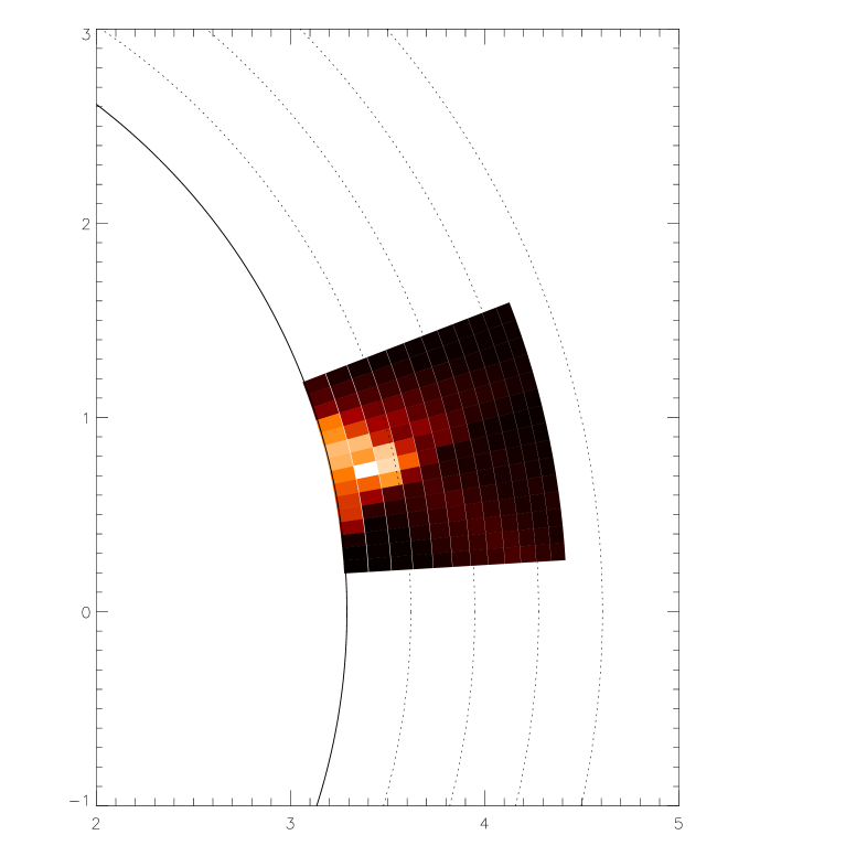
Figure 4: Reconstructed spatial distribution of the flare region on Algol B. All of the flaring plasma has been assumed to be located at a longitude of $\lambda=70^{\circ}$. The circle represents the limb of the K-type star, units are in solar radius; dashed circles indicate heights in steps of 0.1 stellar radii. The system is shown at $\phi$ = 0.5556, when the longitude $\lambda=70^{\circ}$ is viewed at the limb.

As discussed extensively by Lucy (1994), it is somewhat difficult to decide when to stop the iteration in Eq. 4. We followed the recipe given by Lucy (1994) and computed for each iteration the likelihood $H$ (cf. Eq. 3) and solution entropy S (cf. Eq. 5). In Fig. 5 we plot S vs. $H$. There is no clearly identifiable point in the $H$-S diagram where the curvature changes; the solution chosen by us and shown in Fig. 4 is indicated by a large diamond. We also investigated the solution properties of further iterated solutions and found that those pixels with significant flux do not vary substantially in the course of further iterations, while large flux changes are found only in pixels whose flux is so small that they do not substantially contribute to the overall emission.

Figure 5: Entropy (cf. Eq. 5) vs. likelihood (cf. Eq. 3) for the iterated solution. The chosen final solution is indicated by a large diamond.

4 Discussion

4.1 Flare energetics

We first wish to consider the overall energetics of the flare. For this purpose we need to convert the observed count rate into an energy flux. In order to convert from count rate to flux we considered various spectra of active stars (appropriately corrected for photon pile-up) and constructed acceptable model fits to the EPIC data using a combination of individual temperature components. We found the energy conversion factor ECF $=5.4\ 10^{-12}$ erg cm^-2count^-1 to represent a reasonable choice of count rate to energy flux conversion (in the 0.2–10 keV energy band) for active stars. With a distance of 28 pc towards Algol, we then compute a peak X-ray luminosity of $6.7\times 10^{30}$ erg/sec for the flare. The total released X-ray energy E_X can then be computed from the observed decay time of 14.9 ksec as E${}_{\rm tot}\approx 3.6\times 10^{35}$ erg; note, that this value only refers to the energy contained in the exponential decay part of the light curve. Clearly, this flare is rather tiny with only a hundredth of the energy release observed in the giant flare observed by Schmitt & Favata (1999), yet compared to solar flares, the flare is still about a thousand times more energetic than the strongest solar flares observed. As is clear from our reconstructed flare image, the actual size of the flaring region must have been quite small with a height not exceeding one tenth of a stellar radius.

4.2 Size and emission measure of the flaring region

The longitudinal size of our volume elements is - strictly speaking - undetermined. However, assuming that the apparent vertical size scale of the flare agrees with the longitudinal size scale, we deduce a longitudinal size of $\lambda\sim 6^{\circ}$. Our light curve inversions do yield reasonable solutions also for other values than $\phi_{\rm long}=70^{\circ}$, however, the actual value of $\phi_{\rm long}$ cannot differ too much from that value. If $\phi_{\rm long}$ was much larger, the K star would self-occult the flare, and also the rotation of the flare and the apparent motion of the B-type star would be in opposite directions. If $\phi_{\rm long}$ was much smaller, the flare eclipse would start too early unless it is located far above the stellar surface. We therefore adopt - ad hoc - a longitudinal size of $10^{\circ}$ for each of the volume elements, which then leads to a true size of $V_{\rm elem}=1.0\times 10^{30}$ cm^-3 for all the elements. The reconstructed flare image (cf. Fig. 4) results in an effective count rate in each volume element. With Algol’s distance of d=28 pc we can then compute the X-ray luminosity from each volume element through $L_{X,{\rm elem}}$ = CR_elemECF 4$\pi$d². The optically thin cooling function for plasma temperatures at and above 10⁷ K is approximately given by P(T) $\sim 10^{-24.75}$ T^0.25 erg cm³ sec^-1, i.e., it is rather temperature insensitive. Adopting T $\sim 4.5\times 10^{7}$ K, which we determined from spectral fits and also agrees with the values reported by Yang et al. (2003), we can then compute the corresponding emission measure for each volume element through $EM_{\rm elem}=L_{X,{\rm elem}}/$P(T).

4.3 Density of the flaring region

Figure 6: Cumulative density distribution histogram for reconstructed flare image shown in Fig. 4. From the reconstructed intensity in each volume element and its size, the emission measure and electron density can be calculated; shown is the density as a function of the integrated and normalized flare emission measure; see text for details.

Given $V_{\rm elem}$ and $EM_{\rm elem}$ for each volume element, we can compute the plasma density $n_{\rm elem}$ for each volume element using $n_{\rm elem}=\sqrt{EM_{\rm elem}/V_{\rm elem}}$. The resulting density frequency distribution in our volume elements is shown as a function of the total integrated and normalized emission measure in Fig. 6. From Fig. 6 it obvious that the bulk of the flare emission comes from regions with high densities, more than three quarters of the emission measure resides at densities of at least $10^{11}$ cm^-3 and the peak densities reach approximately 2 $\times$ $10^{11}$ cm^-3. With the simultaneously taken XMM-Newton RGS data (with a slightly longer integration time of 52.66 ksec) we can check the densities derived from our light curve inversions. Doing this one must be aware that the bulk of the flaring plasma has a very high temperature (T $\approx$ 45 MK), where essentially no O vii emission is produced, and therefore O vii emission actually provides no information on the main flare component. In Fig. 7 we plot the O vii He-like triplet obtained from the whole observation. The continuum is very high and the weak intercombination and forbidden lines of O vii can hardly be detected above the continuum. We nevertheless extracted spectra during quiescent and flare phases, but we were unable to find significant differences in the f/i ratios. This indicates that either the sensitivity of our data is such that a density enhancement between flaring and quiescent emission is not detectable or that the f/i-ratio is actually dominated by the radiation field of the B-type star (Ness et al., 2002a, b). Given the geometrical configuration at secondary minimum, the observable corona on the K-type star is clearly fully immersed in the B star’s radiation field. When accounting for the radiation field in the way described by Ness et al. (2002b) we estimate the density from our measured f/i ratio f/i = 0.86 $\pm$ 0.37 to $\log\,n_{e}=10.6\,\pm\,1.42$ (and otherwise $\log\,n_{e}=11.1\,\pm\,0.23$). We also note that the f/i-ratios derived for Algol from the Chandra MEG and LETGS and from the XMM-Newton RGS, i.e., from three independent data sets taken at three different times, all agree with each other (to within their respective errors; cf. Ness et al., 2003b), so that at present there is no evidence for phase and/or flare related changes in the O vii f/i-ratio for Algol. Unfortunately, with the XMM-Newton RGS it is not possible to disentangle the contamination due to Fe lines in the Ne ix triplet (cf. Ness et al., 2003a) and signal in the spectrum obtained from the second dispersion order is too low to detect the Ne ix lines. Since the MEG and HEG f/i ratios derived from Chandra observations at different times also do indicate densities in excess of $10^{11}$ cm^-3 (cf. Ness et al., 2003b), we conclude that the densities derived from our light curve inversion are consistent with the available spectroscopic data on Algol.

4.4 Cooling of the flare plasma

An often encountered method to compute densities of a flaring plasma assumes radiative cooling to be the dominant cooling mechanism. Using the relation Doyle et al. (1988)

$$n_{e,rad}=\frac{3kT}{\tau{\rm P(T)}},$$ (6)

where $\tau$ denotes the observed decay time scale of the flare, we compute a density $n_{e,rad}\sim 9\times 10^{10}$ cm^-3 leading to a volume of $V_{rad}\sim 2\times 10^{32}$ cm³, which is of a similar order as the volume derived in our reconstruction. We therefore conclude that radiative cooling may in fact be the dominant cooling mechanism for this particular flare observed on Algol B, in contrast to the flare described by Schmitt & Favata (1999), which cannot have cooled by radiation alone.

Figure 7: O vii triplet obtained from the full XMM-Newton RGS data set; see text for details.

4.5 Magnetic fields

If we assume the post-flare material to be magnetically confined, we can compute the minimal field strength $B_{min}$ required for confinement from

$$\frac{B_{min}^{2}}{8\pi}=2n_{e}kT\,.$$ (7)

Using the values $n_{e}=2\times 10^{11}$ cm^-3 and $T=4.5\times 10^{7}$ K as typical values for density and temperature, we find $B_{min}\approx$250 G. Assuming that the total released energy ultimately comes from reconnected magnetic energy, we can compute the typical reconnected, i.e., non-potential magnetic field strength from

$$\frac{B^{2}_{\rm reconnected}V}{8\pi}=E_{\rm tot}.$$ (8)

Using $V=5\times 10^{31}$ cm³, we find an annihilated field of about 430 G. Of course, since the observed released X-ray energy constitutes only some (small) fraction of the overall released energy, the latter and hence the total reconnected magnetic flux must be larger. If we assume - ad hoc - that only 10% of the released energy ends up as soft X-ray radiation, reconnected field strengths $>1000$ G are required. We therefore conclude that coronal field strengths in excess of 1000 G are present at least in the lower part of Algol B’s corona. Thus a magnetic reconnection scenario for the Algol flare appears fully plausible.

4.6 Quiescent emission

Finally, it is intersting to note, that at the time of first contact, which according to the parameters listed in Tab. 1, is expected to occur at phase $\phi=0.43$ no change in the X-ray light curve is apparent. The light curve stays essentially constant until the flare start at $\phi=0.48$. Eclipses of individual coronal background features might be hidden under the flare-induced count rate increase, however, the smooth overall appearance of the flare light curve provides little support for such an assumption. The mid-eclipse count rates in the energy bands 2–5 keV and 5–10 keV agree very well with those observed prior to flare and eclipse onset, so no eclipses need to be invoked. In the two lower energy bands the mid-eclipse count rates are reduced by about 10% compared to the pre-flare and pre-eclipse rates, on the other hand, the pre-flare and pre-eclipse rates are also somewhat modulated, so again the assumption of an eclipse does not appear to the urgently required. We therefore conclude that the “quiescent” emission from Algol B did not experience any substantial eclipse during our XMM observations and that the vast bulk of the “quiescent” coronal emission remained unocculted during the eclipse, in contrast to the flare which was totally eclipsed.

The absence of any clear eclipse of the “quiescent” emission can be explained either by extended emission or by locating the emission within the unocculted north polar cap. As pointed out above, all of the available spectroscopic density measurements of Algol indicate high densities, thus suggesting that the latter possibility is the far more likely one. With the system parameters listed in Tab. 1, we compute that about 10% of the whole surface remain uneclipsed during the course of the XMM-Newton observations. Since the coronal densities of the quiescent emission is very likely (for a detailed discussion of different density measurements for Algol and other coronal sources we refer to Ness et al., 2003b) not too different from the density of the flaring region, which we know to be located at a height of $\approx 0.1$ R_⋆, we conclude that the “quiescent” emission also comes from rather “compact” regions, which must, however, be located at latitudes $\theta<$ 69^∘ from the north pole. The “southern” eclipsed part of Algol B must have been devoid of any substantial X-ray emission at the time of the XMM-Newton observations. Thus the filling factor of “quiescent” coronal X-ray emission of Algol B must be small, i.e, $f<0.1$. The observed “quiescent” count rate of 25 cts/sec corresponds to an emission measure of $1.3\times 10^{54}$ cm^-3, i.e., only about twice the emission measure of the flaring region. Assuming that the emission comes from the whole of the uneclipsed region, we compute for the product $n_{e}^{2}h=2\times 10^{31}$ cm^-5, where $h$ denotes the average height of the corona. If that average height is the same as that of the flare, i.e, a tenth of a stellar radius, we compute a density of $3\times 10^{10}$ cm^-3. Of course, the filling factor is likely to be smaller, and if the density is indeed $10^{11}$ cm^-3, the overall filling factor on the K-type star is about one percent.

5 Summary

We have observed a flare on Algol B during secondary minimum with complete light curve coverage. The location of the flaring region will be well reconstructed with only some slight ambiguity as to the longitude of the flare occurrence. In particular, the height of the flare above the surface is about 0.1 R_⋆ and the flare did not occur in the polar regions. The plasma densities computed from the observed emission measure and the reconstructed volume agree with each other and are in the range of a few times $10^{11}$ cm^-3. The “quiescent” emission from Algol B was confined to a region at least 20^∘ north of the equator, and only 10% of Algol B’s surface were not occulted at any time during our XMM-Newton observations. If quiescent and flaring regions are located at the same heights, minimal densities of $3\times 10^{10}$ cm^-3 result; smaller filling factors result in correspondingly larger densities as suggested by spectroscopic measurements. Thus, the overall coronal filling factor of Algol B appears to be quite small despite its enormous total X-ray luminosity.