THE PROPAGATION AND ERUPTION OF RELATIVISTIC JETS FROM THE STELLAR PROGENITORS OF GRBs

Abstract

New two- and three-dimensional calculations are presented of relativistic jet propagation and break out in massive Wolf-Rayet stars. Such jets are thought responsible for gamma-ray bursts. As it erupts, the highly relativistic jet core (3 to 5 degrees; $\Gamma\gtrsim 100$) is surrounded by a cocoon of less energetic, but still moderately relativistic ejecta ($\Gamma\sim 15$) that expands and becomes visible at larger polar angles ($\sim$ 10 degrees). These less energetic ejecta may be the origin of X-ray flashes and other high-energy transients which will be visible to a larger fraction of the sky, albeit to a shorter distance than common gamma-ray bursts. Jet stability is also examined in three-dimensional calculations. If the jet changes angle by more than three degrees in several seconds, it will dissipate, producing a broad beam with inadequate Lorentz factor to make a common gamma-ray burst. This may be an alternate way to make X-ray flashes.

1 INTRODUCTION

It is now generally acknowledged that “long-soft” gamma-ray bursts (henceforth, just “GRBs”) are a phenomenon associated with the deaths of massive stars. In addition to the observed association with star-forming regions in galaxies (Vreeswijk et al., 2001; Bloom, Kulkarni, & Djorgovski, 2002; Gorosabel et al., 2003); “bumps” observed in the afterglows of many GRBs (Reichert, 1999; Galama et al., 2000; Bloom et al., 2002; Garnavich et al., 2003; Bloom, 2003); spectral features like a WR-star in the afterglow of GRB 021004 (Mirabal et al., 2002); and the association of GRB 980425 with SN 1998bw (Galama et al., 1998), there is now incontrovertible evidence that at least one GRB (030329) was accompanied by a bright, energetic supernova of Type Ic, SN 2003dh (Price et al., 2003; Hjorth et al., 2003; Stanek et al., 2003). Thus some, if not all GRBs, are produced when the iron core of a massive star collapses either to a black hole (Woosley, 1993; MacFadyen & Woosley, 1999) or a very rapidly rotating highly magnetic neutron star (Wheeler et al., 2000), producing a relativistic jet. Other alternatives in which the GRB occurs after the supernova (Vietri & Stella, 1998) cannot simultaneously explain GRB 030329 and SN 2003dh.

At the same time, the general class of high energy transients once generically called “gamma-ray bursts” has been diversifying. For some time, soft gamma-ray repeaters (SGRs) and “short hard gamma-ray bursts” have enjoyed a distinct status and, presumably, a separate origin. In addition, we now have cosmological “X-ray flashes” (“XRFs”; Heise et al, 2001; Kippen et al., 2003), “long, faint gamma-ray bursts” (in’t Zand et al., 2003), and lower energy events like GRB980425 (Galama et al., 1998). Is a different model required for each new phenomenon, or is some unified model at work, as in active galactic nuclei, a model whose observable properties vary with its environment, the angle at which it is viewed, and perhaps its redshift?

The answer is probably “both”. Even within the confines of the collapsar model, there are Types I, II and III (Heger et al., 2003). Type I happens only in massive stars that make their black holes promptly (MacFadyen & Woosley, 1999). This is what people generally have in mind when they use the word “collapsar”. In Type II though, a similar mass black hole forms by fall back and the burst lasts much longer (MacFadyen, Woosley, & Heger, 2001). Type III, happens only at very low metallicity and requires Pop III stars as its progenitors (Fryer, Woosley, & Heger, 2001). The event is very energetic, but highly redshifted. These other models may be particularly appropriate for unusually long bursts. A jet that wavered in its orientation in any of these events would emerge with a greater load of baryons. So would a jet whose power declined in a time less than that required to traverse the star. A jet in a blue supergiant would become choked because the power of the central engine has decreased substantially when the jet is still deep inside the star. Thus any sort of collapsar happening in a blue supergiant instead of a Wolf-Rayet star would produce a different sort of transient. Finally, it may just be that jets are just born with different baryon loadings, perhaps relating to the mass of the presupernova star and its distribution of angular momentum and magnetic field. Our present understanding of nature allows for all these solutions.

However, it also seems to reason that not all jets are the same, even for Type I collapsars, and that even if they were, different phenomena would be seen at different angles. We are thus motivated to consider the observational consequences of highly relativistic jets as they propagate through, and emerge from massive stars. What would they look like if seen from different angles? In particular, what is the distribution with polar angle of the energy and Lorentz factor? Might softer, less energetic phenomena be observed off axis and with what frequency?

Jets inside massive stars have been studied numerically in both Newtonian (MacFadyen & Woosley, 1999; MacFadyen, Woosley, & Heger, 2001; Khokhlov et al., 1999) and relativistic simulations (Aloy et al., 2000; Zhang, Woosley, & MacFadyen, 2003, henceforth Paper 1) and it has been shown that the collapsar model is able to explain many of the observed characteristics of GRBs. These previous studies have also raised issues which require further examination, especially with higher resolution. For instance, the emergence of the jet and its interaction with the material at the stellar surface and the stellar wind could lead to some sort of “precursor” activity. The cocoon of the jet will also have different properties from the jet itself and shocks within the cocoon or with external matter could lead to $\gamma$-ray and hard X-ray transients (Ramirez-Ruiz, Celotti, & Rees, 2002). There is also the overarching question of whether jets, calculated in two dimensions with assumed axial symmetry, are stable when studied in three dimensions.

Here we examine in two- and three-dimensional numerical studies, the interaction of relativistic jets with the outer layers of the Wolf-Rayet stars thought responsible for GRBs. We follow the emergence of the jets for a sufficient length of time to ascertain the properties of the cocoon explosion that surrounds the GRB and we study the dependence of the results on the dimensionality of the calculation. Such explosions are visible to a much greater angle and to a much larger number of observers. The observed phenomenon could be a hard X-ray flash or a weak GRB. We also find that the properties of the emergent jet are quite sensitive to whether the jet maintains its orientation (to within a critical angle) for durations of $10\,{\mathrm{s}}$ or so, the time it takes the jet to traverse the star. Jets that waiver may make hard transients of some sort, but not GRBs.

2 Stellar Model and Numerical Methods

2.1 Progenitor Star

A collapsar is formed when the iron core of a rotating massive star collapses to a black hole and an accretion disk. The interaction of this disk with the hole, through processes that are still poorly understood, produces jets with a high energy to mass ratio. Here we are concerned primarily with the propagation of these relativistic jets, their interactions with the star and the stellar wind, and the observational implications, and not so much with how they are born. In fact, our results here would be the same if the jet were produced by some other means (Wheeler et al., 2000) inside the same star.

Unlike in our previous study (Paper 1), the initial stellar model is taken directly from a presupernova star with a very finely zoned surface (Table 1; Fig. 1). Because we are only interested in events that happen outside about $10^{10}\,{\mathrm{cm}}$ on a time scale of, at most, tens of seconds, modification of the initial star by core collapse and rotation is negligible. Specifically, our initial model is a $15\,{\mathrm{M}_{\odot}}$ helium star calculated by Heger & Woosley (2003). This helium star has been evolved to iron-core collapse while following the transport of angular momentum and including the effects of rotational mixing as in Heger, Langer, & Woosley (2000). The initial star was a nearly pure helium star rotating rigidly with a surface velocity equivalent to 10% Keplerian. This is a typical value in the study of Heger, Langer, & Woosley (2000). Presumably the star lost its envelope to a companion early in helium burning. Further mass loss and the transport of angular momentum by magnetic fields were ignored so as to form a big iron core that would very likely collapse to a black hole and give ample angular momentum for a disk. The radius of the helium star at onset of collapse is $8.8\times 10^{10}\,{\mathrm{cm}}$ and the surface of the star is very finely zoned (surface zoning $\lesssim 10^{21}\,{\mathrm{g}}$). Despite the fact that angular momentum transport was followed in the initial model to show its suitability as a collapsar (Fig. 1), rotation plays no role in the present study.

Outside the star, the background density, which comes from the stellar wind, is assumed to scale as $R^{-2}$. The actual value of this density, unless it is very high, plays no role in determining the final answer at the small scales considered here ($<2\times 10^{12}$ cm), but finite value is needed in order to stabilize the code. We assumed a value at $R=10^{11}\,{\mathrm{cm}}$ of $5\times 10^{-11}\,{{\mathrm{g}}\,{\mathrm{cm}}^{-3}}$, where $R$ is the distance from the center of the star. This corresponds to a mass loss rate of $\sim 1\times 10^{-5}\,{{\mathrm{M}_{\odot}}\,{\mathrm{yr}}^{-1}}$ for a wind velocity of $\sim 1000\,{{\mathrm{km}}\,{\mathrm{s}}^{-1}}$ at $10^{11}\,{\mathrm{cm}}$. This mass loss rate is rather low for typical Wolf-Rayet stars of this mass in our galaxy (Nugis & Lamers, 2000), but might be more appropriate for the low metallicity in the GRB neighborhood (Crowther et al., 2002). A small value was also taken in order to be consistent with the assumed progenitor structure that was calculated with zero mass loss.

2.2 Computer Code

We employed a multi-dimensional relativistic hydrodynamics code that has been used previously to study relativistic jets in the collapsar environment (Paper 1). Briefly, our code employs an explicit Eulerian Godunov-type shock-capturing method (Aloy et al., 1999). The governing equations of relativistic hydrodynamics with a causal equation of state can be written as a system of conservation laws for rest mass, momentum, and energy. To solve the equations numerically, each spatial dimension is discretized into cells. Using the method of lines, the multi-dimensional time-dependent equations can then be evolved by solving the fluxes at each cell interface. In order to achieve high order accuracy in time, the time integration is done using a high order Runge-Kutta scheme (Shu & Osher, 1988), which involves prediction and correction. An approximate Riemann solver (Aloy et al., 1999) using the Marquina’s algorithm is used to compute the numerical fluxes from physical variables: pressure, rest mass density, and velocity at the cell interface. The values of the physical fluid variables at the cell interface are interpolated using reconstruction schemes (e.g., piecewise parabolic method, Colella & Woodward, 1984). This reconstruction procedure ensures high order accuracy in spatial dimensions. The conserved variables: rest mass, momentum and energy are evolved directly by the scheme. In each time step, physical variables, such as pressure, rest mass density and velocity, which are necessary in calculating the numerical fluxes, can be recovered from conserved variables by Newton-Raphson iteration. The code can operate in Cartesian, cylindrical, or spherical coordinates. Approximate Newtonian gravity is implemented by including source terms in the equations. Total energy, which includes kinetic and internal energy, in the laboratory frame are not exactly conserved due to gravitational potential energy and the way of implementing gravity as source terms. However, the code conserves energy to machine precision when gravity is turned off. Furthermore, the gravitational potential energy is negligible for relativistic material in our calculations. For instance, assuming a $10\,{\mathrm{M}_{\odot}}$ central point mass, a fluid element with a velocity of $0.5\,c$ at the inner boundary of our computational grids, $10^{10}\,{\mathrm{cm}}$ (§ 3.1, § 4.1), has potential energy of less than 0.1% of its kinetic energy. Thus we expect that our calculations conserve energy to an accuracy of better than 0.1%. In simulations present in this paper, A gamma-law equation of state with $\gamma=4/3$ is used for the simulations presented in this paper.

3 Two-Dimensional Models

3.1 Model Set Up and Definitions

The mass interior to $1.0\times 10^{10}\,{\mathrm{cm}}$ is removed from the presupernova star and replaced by a point mass. No self gravity is included. This should suffice since we are studying phenomena that happen on a relativistic time scale and the speed of sound is very sub-luminal. While jets presumably go out both axes, we follow here only one, assuming symmetry in the other hemisphere. Jets are injected along the rotation axis (the center of the cylindrical axis of the grid) through the inner boundary. Each jet is defined by its power (excluding rest mass energy), $\dot{E}$, its initial Lorentz factor, $\Gamma_{0}$, and the ratio of its total energy (excluding rest mass energy) to its kinetic energy, $f_{0}$. Our previous studies in Paper 1 have shown that a jet that starting with a half-opening angle of $20\arcdeg$ and a high Lorentz factor, $\Gamma\sim 50$ at $2000\,{\mathrm{km}}$, will be shocked deep inside of the star. By the time it reaches $10^{10}\,{\mathrm{cm}}$, a jet should have a large ratio of internal energy to rest mass, a half-opening angle of about $5\arcdeg$, and a Lorentz factor, $\Gamma\sim 5-10$.

Though GRBs observationally have highly variable properties, the jet power was taken here to be constant for the first $20\,{\mathrm{s}}$, then turned down linearly during the next 10 seconds. That is, during the interval 20 to 30 s, the power scaled as $(30\,{\mathrm{s}}-t)/10\,{\mathrm{s}}$ decreasing to zero at $30\,{\mathrm{s}}$. During the declining phase, the pressure and density remained constant, and the Lorentz factor was calculated from the internal energy, density, and power. After 30 seconds, a pure outflow boundary condition was used for the inner boundary. The axis of the jet is defined as the $z$-axis in all cases and the jets were initiated parallel to that axis in a region that subtended a half-angle of 5 degrees as viewed from the origin.

Four models were calculated which span a range of energies and Lorentz factor (Table 2). In Model 2A, a total energy of $\sim 5\times 10^{51}\,{\mathrm{erg}}$ is injected, comparable to the results of Frail et al. (2001), but larger than the results of Panaitescu & Kumar (2001) by an order of magnitude (Table 3). In Models 2B and 2C, higher and lower energy deposition rates were employed. For the parameters chosen, a jet with an initial Lorentz factor of 5 or 10 at $10^{10}\,{\mathrm{cm}}$ should have a final Lorentz factor of $\sim 180-200$ if all internal energy is converted into kinetic energy. The zoning employed in the models is given in Table 4. Typically over three million zones were used.

Model 2C used an extended grid in the $r$-direction, which allowed the greater lateral expansion of the jet to be followed at late times. This was necessary because of its lower energy and greater expansion during the time it took to traverse the extent of the $z$-grid. Model 2T used conditions like those of Model 2B, but a grid that was both smaller and coarser, chosen to be equivalent to that used in the three-dimensional calculations described later in the paper (§ 4).

3.2 Results in Two Dimensions

The relativistic jet begins to propagate along the $z$-axis shortly after its initiation. In agreement with previous studies (Aloy et al., 2000, and Paper 1), the jet consists of a supersonic beam, a shocked cocoon, a bow shock, and is narrowly collimated. Some snapshots of Models 2A, 2B, and 2C are given in Figs. 2, 3, and 4. The resulting “equivalent isotropic energies” for matter exceeding a certain Lorentz factor are also given, at $70\,{\mathrm{s}}$, for the same three models in Figs. 5, 6, and 7. The latter figures also give the estimated terminal Lorentz factor assuming that internal energy along the radial line of sight is converted into kinetic energy. The equivalent isotropic energy is defined as that energy an isotropic explosion would need in order to give the calculated flux of energy along the line of sight. It is a way of mapping the highly asymmetric two-dimensional results into equivalent one-dimensional models. The change in Lorentz factor between $70\,{\mathrm{s}}$ and infinity is not very great, except in situations where matter that was highly relativistic to begin with receives an additional boost in its frame by expansion. The duration of the calculation was set by how long it took the jet to reach the end of the simulation grid and would be costly to increase, but as the figures show, especially in Model 2C, there was still an interesting amount of internal energy at $70\,{\mathrm{s}}$.

The fractions of energies inside a certain angle to the total energies on the grid are given in Fig. 8. In all cases studied the high Lorentz factor characteristic of common GRBs is confined to a narrow angle of about 3 to 5 degrees with a maximum equivalent isotropic energy in highly relativistic matter along the axis of $\sim 3\times 10^{53}$ to $3\times 10^{54}\,{\mathrm{erg}}$. At larger angles there is significant energy, though, and Lorentz factor, $\Gamma\sim$ 10 to 20. At an angle of 10 degrees for example, the equivalent isotropic energy in matter with $\Gamma>20$ is $\sim 10^{52}\,{\mathrm{erg}}$ in Model 2A and even $10^{51}\,{\mathrm{erg}}$ in Model 2C. At larger angles there is less energy, but still the possibility of low power transients of hard radiation. Model 2B did not eject much material with $\Gamma\gtrsim 10$ at angles $\sim 10$ degrees. The equivalent isotropic energy at larger angles ($>2\arcdeg$) for all three models can be fit well by a simple power-law, $E_{0}\times(\theta/2\arcdeg)^{-3}\,{\mathrm{erg}}$, where $E_{0}$ is $1.5\times 10^{54}$, $4.5\times 10^{54}$ and $6.8\times 10^{53}$, for models 2A, 2B and 2C, respectively. The ratios of the values of $E_{0}$, $1.5:4.5:0.68$, are very close to those of the energy deposition rates, $1.0:3.0:0.5$. Inside $2\arcdeg$, the distributions of energy and Lorentz factor are roughly flat, $\sim E_{0}$. The values of $E_{0}$ can be roughly estimated from the total injected energy and the percentage of the energy in the jet core. For example, about $40\%$ of the total energy on the grid is contained inside 2 degrees for Model 2A (Fig. 8). About $5\times 10^{51}\,{\mathrm{erg}}$ (Table 2) was injected for both jets in Model 2A. One can estimate that the equivalent isotropic energy inside 2 degrees is $\sim 1.6\times 10^{54}\,{\mathrm{erg}}$ for Model 2A. More models need to be calculated to find how the distributions of energy and Lorentz factor at breakout depend on initial conditions.

Table 3 gives the energies for various components of the ejecta at a time $40\,{\mathrm{s}}$ after the jet was initiated. There still remains considerable internal energy available for conversion to kinetic at this time (which was chosen as a time when most of the relativistic matter was still on the grid), but this will affect mostly the matter with high Lorentz factor, $\Gamma>10$. The results show that most of the energy injected as jets at $10^{10}\,{\mathrm{cm}}$ emerges in matter that is still relativistic. Only a small fraction goes into sub-relativistic expansion, nominally $v<0.5\,c$ and consequently, only a little of the jet energy is used to blow up the star. If there were no other energy sources the kinetic energy of the supernova would be $\lesssim 2\times 10^{51}$ erg.

The total energy of relativistic ejecta is also useful for comparison to radio observations of the afterglows of GRBs. For example, Li & Chevalier (1999) have placed limits on the total energy of ejecta with $v>0.5\,c$ in SN 1998bw. The limit, $3\times 10^{50}\,{\mathrm{erg}}$, may be an approximate estimate of the actual energy. The corresponding energy for Model 2C here is four times larger (Table 3). It seems likely that lower energy models than Model 2C could be constructed that would still give high Lorentz factors and equivalent isotropic energies in a narrow range of angles around the polar axis. That is, GRB 980425 may have been a harder, more energetic GRB seen off axis. However, the low energy of that burst, some five orders of magnitude less that that expected for a centrally observed GRB (Fig. 4) remains surprising. Either GRB 980425 was observed at a polar angle larger than 15 degrees, or the burst was weaker at all angles because of baryon loading (§ 1; Woosley, Eastman, & Schmidt 1999).

The possibility that the off-axis emission from material with $\Gamma\sim$ 10 to 20 corresponds to XRFs is discussed in § 5.

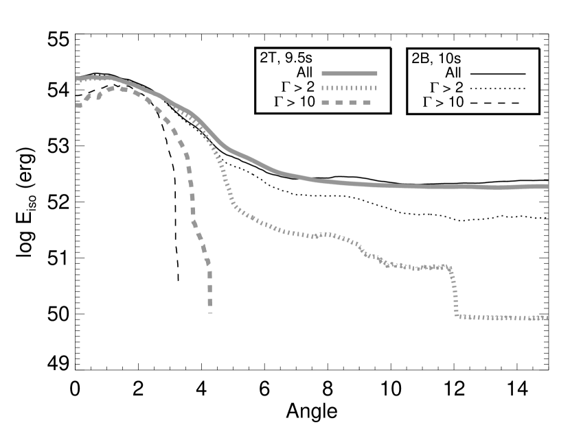
In 2D simulations with cylindrical coordinates, there is an imposed symmetry axis of the coordinate system. It is very important to repeat these calculations in 3D to ensure that our 2D results are valid and to examine three-dimensional jet instabilities. Three-dimensional calculations are, however, computationally expensive. So we have to use lower resolution for 3D calculations. In order to compare 2D and 3D results with the same resolution and identical initial parameters, we did a lower resolution 2D run, Model 2T (Tables 2 and 4). A comparison of two- and three-dimensional results will be discussed in § 4. It is also interesting to compare Model 2B and 2T, which had identical parameters but in different resolution. Qualitatively the results are similar. In both models, the jet emerges from the star with a cocoon surrounding the jet beam and a dense “plug” at the head of the jet (Fig. 9). There are, however, noticeable differences, as we expected. In particular, it takes less time for the jet in Model 2T to emerge from the star than that in Model 2B, because they have different numerical viscosity. The larger numerical viscosity in Model 2T is due to its lower resolution. Despite morphologic differences between Model 2B and 2T (Fig. 9), the energetics of these two models are quite similar (Table 5, Fig. 10). The distributions of equivalent isotropic energy versus angle for the jet core ($\lesssim 3$ degrees) in Models 2B and 2T are very similar. However, Model 2B has more mildly relativistic material ($2<\Gamma<10$) in its cocoon than Model 2T.

4 Three-Dimensional Models

For the three-dimensional models, the same helium star was remapped into a three-dimensional Cartesian grid. Because of the greater cost of computations, these studies covered only an interval of $10\,{\mathrm{s}}$, adequate to watch the jet propagate, develop a cocoon and break out, but not long enough to study the the expansion after break out to any great extent.

4.1 Model Definitions

The parameters of the jet, its power, Lorentz factor and energy loading, were all identical to those of Model 2B, that is $\Gamma=5$, $\dot{E}=3\times 10^{50}\,{{\mathrm{erg}}\,{\mathrm{s}}^{-1}}$ and $f_{o}=40$ (Table 6). The grid employed in all cases was Cartesian with 256 zones each along the $x$- and $y$-axes and 512 along the $z$-axis (jet axis) (Table 7).

The initial model and the initiation of the jet in Model 3A were perfectly symmetric with regard to the axis of the jet. The perfect symmetry was maintained in the calculation because our numerical scheme did not break any symmetry. In order to break the perfect symmetry of the cylindrical initial conditions, an asymmetric jet was injected in Models 3BS and 3BL. At the base of the jet in Model 3BS, pressure and density were 1% more than those of Model 3A if $y\geq{\tan{\alpha}}\,x$, and 1% less otherwise, where $\alpha=40$ degrees. Hence the jet in Model 3BS has a $\pm 1\%$ imbalance in power. In Model 3BL, a $\pm 10\%$ imbalance in power was employed.

Several other models were calculated to explore the collimation properties of non-radial jets that precessed. These jets were initiated at the same $10^{10}\,{\mathrm{cm}}$ inner boundary with a half-angle of 5 degrees as measured from the center. However, they were given a non-$z$ (symmetry axis) component of momentum that would have resulted, in a vacuum, in a propagation vector inclined to the $z$-axis by 3 degrees (Model 3P3), 5 degrees (Model 3P5), and 10 degrees (Model 3P10). The jet precessed around the $z$-axis with a period, in all cases of $2\,{\mathrm{s}}$. This period was chosen to be short compared with the time it took the jet to traverse the remaining star between $10^{10}\,{\mathrm{cm}}$ and the surface, yet long enough that the jet would still be distinct from a cone.

4.2 Breakout in Three Dimensions

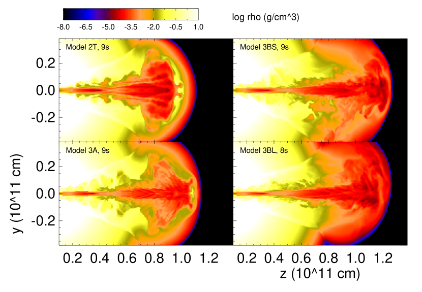
As expected, Model 3A closely resembles Model 2T (Fig. 11). The initial stellar model, the zoning (Tables 4 and 7), and the jet parameters (Tables 2 and 6) were all the same. In particular, the initial conditions for the jet have cylindrical symmetry in both cases. It is gratifying that the answer is insensitive to the dimensionality of the grid, which in Model 2T, was two-dimensional cylindrical and, in Model 3A, was three-dimensional Cartesian. This implies that the bulk properties of jets calculated in Paper 1 - including collimation and modulation - would be the same in 3D.

However, Model 3A, by assuming a jet that initially has perfect cylindrical symmetry does not fully exercise the 3D code. Aside from numerical noise, the equations conserve the 2D symmetry of the initial conditions, even on a 3D grid. Fig. 11 also compares, at breakout, the properties of jets that were, initially, nearly identical. In particular, Model 3BS differed from 3A only in a 1% asymmetry in input energy from one side of the jet to the other, yet the structure of the emergent jet and cocoon is strikingly different. In Model 3BL with a 10% asymmetry the difference is even more striking. The plots show a cross section of the Cartesian grid along the initial jet axis in the $x$ = 0 plane. Because of the 40 degree offset (§ 4.1), there is somewhat more energy in the top half of the figure than the bottom. Though both jets retain high Lorentz factors in their cores, similar to Models 2T and 2B, the cocoon explosion is a little earlier and larger on the top. More dramatic is the difference in the high density “plug” among Models 3A, 3BS, and 3BL. In the latter two where the 2D symmetry was mildly broken, the plug has a much lower density and is not prominent. In 2D models and symmetric 3D Model 3A, the plug is held by a concave surface of the highly relativistic jet core. Because of the imposed axisymmetry, the plug cannot easily escape and is pushed forward by the jet beam. Whereas the story of the plug is different in asymmetric 3D Models 3BS and 3BL. In these models, where the 2D symmetry was initially mildly broken, instabilities will develop. The forward bow shock is no longer symmetric and even the stellar material on the axis is pushed sideways. More importantly, the head of the highly relativistic jet beam is also asymmetric and does not have a concave surface to “hold” the plug. A movie of these runs shows the plug forming, slipping off to the side, then forming again. The plug in these models has a much lower density and is not prominent. The presence or absence of this plug may have important implication for the production of short-hard gamma-ray bursts in the massive star models (Paper 1; Waxman & Mészáros, 2003).

4.3 Stability of the Jet

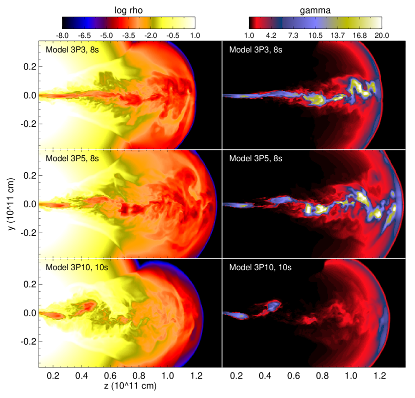
Given the ability to model jets in 3D, we undertook a study to test their survivability against non-radial instabilities. Three jets were introduced on the standard grid (Table 7) with inclinations to the radial of 3, 5, and 10 degrees (Table 6). These jets were made to precess with a period equal to $2\,{\mathrm{s}}$, i.e., a non-trivial fraction of the time it takes the jet to traverse the star and break out. The results are shown in Fig. 12.

With an angle of 3 degrees, the jet in Model 3P3 escapes the star with its relativistic flow at least partly intact. Though Fig. 12 shows Lorentz factors of only $\Gamma\sim 10-20$, the internal energy is still very large and some of these regions will attain $\Gamma\sim 180$ if they expand freely. However, there is some “baryon-poisoning”. No clear line of sight exists along a radial line for the most energetic material even in the jet beam. Perhaps a jet with intermediate Lorentz factor would emerge. We have not yet followed these calculations to large radius (as in Figs. 2, 3, and 4) because the 3D grid was not large enough. Larger calculations are planned.

At larger angles Model 3P5 and especially 3P10 show the break up of the jet. Because there is no well focused highly relativistic jet beam, especially in Models 3P5 and 3P10, more baryon mass is mixed into the jet. The Lorentz factor of the jet will decrease due to dissipation. And it will be very difficult for these jets to make a common GRB. Again some sort of hard transient might be expected, especially after all the internal energy converts and $\Gamma$ rises, but for Model 3P10 there will be no GRB of the common variety. In our simulations, we find that the critical angle for jet precession is about 3 degrees. One would expect that the constraint on the angle of precession will be reduced if the jet bears more power or is powered longer.

Is two seconds a reasonable period for the jet to precess? There are many uncertainties, but the gravitomagnetic precession period of a black hole surrounded by an accretion disk is estimated by Hartle, Thorne, & Price (1986) to be

$$T_{\mathrm{GM}}=900(M_{\mathrm{disk}}/0.001\,{\mathrm{M}_{\odot}})^{-1}(M_{\mathrm{bh}}/3\,{\mathrm{M}_{\odot}})^{-1/2}(r/300\,{\mathrm{km}})^{2.5}\,{\mathrm{s}},$$

where $M_{\mathrm{disk}}$ is the mass of the accretion disk, $M_{\mathrm{bh}}$ is the mass of the hole and $r$ is the radius of the disk. $r=300\,{\mathrm{km}}$ is a reasonable value for the radius of the disk, which depends on the distribution of angular momentum of the star (MacFadyen & Woosley 1999). The dependence of the mass in the disk on the alpha-viscosity has been explored in both numerical simulations (MacFadyen & Woosley 1999) and analytic calculations (Popham, Woosley & Fryer 1999). For currently favored value of the alpha-viscosity, $\sim 0.1$, the disk mass is about $0.001\,{\mathrm{M}_{\odot}}$. For the disk mass to approach $1\,{\mathrm{M}_{\odot}}$ the viscosity would need to be $\alpha<0.001$. Given the low mass of the accretion disk and the radius of the disk, $\sim 300\,{\mathrm{km}}$, precession periods as small as two seconds are unlikely, but the black hole may be kicked or instabilities deeper in the region of the star not modeled here could give the jet some non-radial component. If so, Fig. 12, shows an alternate way in which baryon-loaded jets could give rise to less relativistic mass ejected and slower moving jets far away from the star($10\lesssim\Gamma\lesssim 100$). Softer transients like XRFs and sub-luminous GRBs like GRB 980425 could result.

5 Discussion

Our calculations show, so long as the orientation of the jet does not waiver on time scales of order seconds by angles greater than 3 degrees, that a relativistic jet can traverse a Wolf-Rayet star while retaining sufficient energy and Lorentz factor to make a GRB. This conclusion is robust in three dimensions as well as two.

As it breaks out, the jet is surrounded by a cocoon of mildly-relativistic, energy-laden matter. As internal energy converts to kinetic, matter with $10^{51}$ to $10^{52}\,{\mathrm{erg}}$ of equivalent isotropic energy moving with Lorentz factor $\Gamma\gtrsim 20$ is ejected to angles about three times greater than the GRB. That is, whatever transient the cocoon gives rise to will be an order of magnitude more frequently observable in the universe, but two orders of magnitude less energetic than a GRB. Weaker transients can of course be obtained at still larger angles and there is considerable diversity in the models (Figs. 5, 6, and 7).

The isotropic equivalent rest mass to $10^{51}$ - $10^{52}\,{\mathrm{erg}}$ with $\Gamma\approx 20$ is $3\times 10^{-5}$ to $3\times 10^{-4}\,{\mathrm{M}_{\odot}}$. This matter would give up its energy upon encountering $1/\Gamma$ times its rest mass. For an assumed mass loss rate for the Wolf-Rayet progenitor of $10^{-5}\,{{\mathrm{M}_{\odot}}\,{\mathrm{yr}}^{-1}}$ and speed, $1000\,{{\mathrm{km}}\,{\mathrm{s}}^{-1}}$, the energy will be radiated at about $3\times 10^{14}$ to $3\times 10^{15}\,{\mathrm{cm}}$. Emission from this deceleration will have a duration $\sim R/(2\Gamma^{2}c)\sim$ 10 - $100\,{\mathrm{s}}$. Variations of a factor of 10 are easily achievable by varying the mass loss rate or Lorentz factor.

Unlike the central jet, we do not see evidence for large scale variation in the Lorentz factor at lower latitude and so it would be hard to make the transient emission by internal shocks. We thus attribute the emission to external shocks and invoke a variety of Lorentz factors emitting within our light cone in order to explain the spread in wavelength.

Might there be observable counterparts to these large angle, low Lorentz factor explosions? Typically, they have too low a Lorentz factor to make common GRBs (Guetta, Spada, & Waxman, 2001). Tan, Matzner, & McKee (2001) present arguments however that, by external shock interaction with the progenitor wind, a hard transient of some sort should result.

Our model predicts a correlation between $E_{\rm iso}$, the Lorentz factor, and the angle between the polar axis and the observer (Fig. 5, 6 and 7). Roughly speaking, the GRB outflows have a narrow highly relativistic jet beam and a wide mildly relativistic jet wing. Recent observations and afterglow modeling support this non-uniform jet model (Berger et al., 2003; Zhang et al., 2003; Salmonson, 2003; Rossi, Lazzati, & Rees, 2002). If, as seems reasonable, the Lorentz factor is, in turn, correlated with the peak energy observed in the burst one expects a continuum of high energy transients spanning the range from X-ray afterglows (keV), to hard X-ray transients (tens of keV), to GRBs (hundreds of keV). Observations reviewed by Amati et al. (2002) show such a correlation for bursts with $E_{\rm peak}$ from 80 keV to over 1 MeV and Lamb (private communication) finds that the relation extends to the lower energies.

In particular, XRFs form a new class of X-ray transients having a duration of order minutes and properties that in ways resemble GRBs (Heise et al, 2001; Kippen et al., 2003). XRFs are probably many phenomena (Arefiev, Priedhorsky, & Borozdin, 2003) and it could be that, especially some of the longer ones, have alternate explanations (see introduction). However, we have felt for some time (Woosley, Eastman, & Schmidt, 1999; Woosley & MacFadyen, 1999; Woosley, 2000, 2001, Paper 1) that many XRFs are the off-axis emissions of GRBs, made in the lower energy wings of the principal jet. We have not calculated the expected spectra for any of our models, only Lorentz factors and energies. However, it is reasonable that matter moving with $\Gamma\sim$ 20 would make a transient softer than a GRB and harder than a few keV. Larger amounts of energy are emitted at a larger range of angles for slower but still relativistic ejecta ($\Gamma=5$, e.g., Fig. 5).

If our model is valid, XRFs and GRBs should be continuous classes of the same basic phenomenon sharing many properties. They should have a similar spatial distribution to GRBs because they are essentially the same sources. However, because they are much less luminous, their log N-log S distribution would not exhibit the same roll over attributed in GRBs to seeing the “edge” of the distribution (e.g., Fishman & Meegan 1995). Their median redshift should be considerably smaller, certainly less than 1. This is consistent with the low redshifts inferred for the host galaxies of two XRFs by Bloom et al. (2003). XRFs may, most frequently, be seen in isolation and will be characterized by softer spectra, but there would also be an underlying XRF in every GRB since the emission of the mildly relativistic cocoon material is beamed to a larger angle that includes the poles. In some cases these XRFs might be seen as precursors or extended hard X-ray emission following a common GRB. They should be associated with supernovae. Indeed XRFs may more frequently serve as guideposts to jet-powered supernovae than GRBs, especially the nearby ones.

Though considerable variation is expected, our calculations (e.g., Fig. 5) suggest that XRFs are typically visible at angles about three times greater than GRBs and hence to ten times the solid angle. However, their energy, a few percent of GRBs, implies that a flux-limited sample could observe GRBs out to roughly ten times farther, implying that XRFs would be about 1% as frequent in the sample. The actual value is detector sensitive, but may be larger.

One should also keep in mind the possibility that XRFs do not accompany GRBs, in any direction, but are a result of baryon loading of the central jet. Three-dimensional instabilities (Fig. 12) may play an important role in this and are being explored.

Table 1: Properties   of the Progenitor Model

	m	r	J
	(${\mathrm{M}_{\odot}}$)	(${\mathrm{cm}}$)	(${\mathrm{erg}}\$s)
iron core	1.95	$2.58{{\times}{10^{8}}}$	$1.23{{\times}{10^{50}}}$
Si core	2.61	$4.99{{\times}{10^{8}}}$	$2.35{{\times}{10^{50}}}$
Ne/Mg/O core	2.95	$7.06{{\times}{10^{8}}}$	$2.68{{\times}{10^{50}}}$
C/O core	8.56	$5.16{{\times}{10^{9}}}$	$2.24{{\times}{10^{51}}}$
star / He core	15.00	$8.80{{\times}{10^{10}}}$	$1.00{{\times}{10^{52}}}$

Table 2: Parameters of 2D-Models

	$\dot{E}$			$z_{0}$	$T_{1}$	$T_{2}$	$E_{\mathrm{tot}}$
Model	($10^{50}\,{{\mathrm{erg}}\,{\mathrm{s}}^{-1}}$)	$\Gamma_{0}$	$f_{0}$	($10^{10}\,{\mathrm{cm}}$)	(${\mathrm{s}}$)	(${\mathrm{s}}$)	($10^{51}\,{\mathrm{erg}}$)	Grid
2A	1.0	10	20	1.0	20	10	5.0	Normal
2B	3.0	5	40	1.0	20	10	15.0	Normal
2C	0.5	5	40	1.0	20	10	2.5	Large
2T	3.0	5	40	1.0	20	10	15.0	Coarse

Table 3: Energetics of 2D-Models

Model	Energy input	Total on grid	$v>0.5\,c$	$\Gamma>2$	$\Gamma>10$
	(1051 erg)	(1051 erg)	(1051 erg)	(1051 erg)	(1051 erg)
2A	5.0	4.66	3.64	3.56	3.32
2B	15	14.36	12.46	12.22	11.16
2C	2.5	1.93	1.20	1.13	0.92

Table 4: Zoning in 2D-Models ($10^{10}\,{\mathrm{cm}}$)

Model	$r_{1}$	$r_{2}$	$r_{3}$	$z_{1}$	$z_{2}$	$z_{3}$	$r$	$z$
	$\Delta r_{1}$	$\Delta r_{2}$	$\Delta r_{3}$	$\Delta z_{1}$	$\Delta z_{2}$	$\Delta z_{3}$	zones	zones
2A	10.0	20.0	60.0	10.0	20.0	200	1500	2275
	0.01	0.04	0.16	0.01	0.04	0.16
2B	10.0	20.0	60.0	10.0	20.0	200	1500	2275
	0.01	0.04	0.16	0.01	0.04	0.16
2C	10.0	20.0	200.0	10.0	20.0	200	2375	2275
	0.01	0.04	0.16	0.01	0.04	0.16
2T	0.64	3.84	-	13.8	-	-	256	512
	0.01	0.05	-	0.025	-	-

Table 5: Energetics of 2D-Models 2B and 2T

Model	Energy input	Total energy	$v>0.5\,c$	$\Gamma>2$	$\Gamma>10$
	(1051 erg)	(1051 erg)	(1051 erg)	(1051 erg)	(1051 erg)
2B	3	2.46	1.44	1.31	0.51
2T	2.85	2.42	1.50	1.13	0.52

Table 6: Parameters of 3D-Models

	$\dot{E}$			$z_{0}$	$\theta_{p}$	Period
Model	($10^{50}\,{{\mathrm{erg}}\,{\mathrm{s}}^{-1}}$)	$\Gamma_{0}$	$f_{0}$	($10^{10}\,{\mathrm{cm}}$)	(degrees)	(${\mathrm{s}}$)
3A	3.0	5	40	1.0	0	-
3BL	3.0	5	40	1.0	0	-
3BS	3.0	5	40	1.0	0	-
3P3	3.0	5	40	1.0	3	2
3P5	3.0	5	40	1.0	5	2
3P10	3.0	5	40	1.0	10	2

Table 7: Zoning in 3D-Models ($10^{10}\,{\mathrm{cm}}$)

$x_{1}$	$x_{2}$	$y_{1}$	$y_{2}$	$z_{1}$	$x$	$y$	$z$
$\Delta x_{1}$	$\Delta x_{2}$	$\Delta y_{1}$	$\Delta y_{2}$	$\Delta z_{1}$	zones	zones	zones
0.64	3.84	0.64	3.84	13.8	256	256	512
0.01	0.05	0.01	0.05	0.025

Figure 1: Structure of the star at the onset of core collapse as a function of enclosed mass, $m$. Panel A gives mass fractions of the dominant species, Panel B density ($\rho$) and temperature ($T$) stratification, and Panel C angular velocity ($\omega$) and average specific angular momentum on spherical shells ($j$). The enclosed mass at $10^{10}\,{\mathrm{cm}}$, where the jets were launched in our simulations, is $10.3\,{\mathrm{M}_{\odot}}$.

Figure 2: Time evolution of the density (bottom of each frame) and Lorentz factor (top of each frame) in the jet and its environs for Model 2A. The density is on a logarithmic scale, the Lorentz factor is on a linear scale, both color coded. Quantities are given 5, 10, 12, 20, 40, and 70 s after the initiation of the jet at $0.1\times 10^{11}\,{\mathrm{cm}}$. The third panel at 12 s is just as the jet is erupting from the star (radius $0.89\times 10^{11}\,{\mathrm{cm}}$). By 70 s, most of the internal energy has converted to kinetic and the Lorentz factor has almost reached its terminal value. Values of $\Gamma$ at this time in the central, over-exposed jet are near 150. Note the explosion of the cocoon as the jet erupts and the ejection of material with terminal Lorentz factor, $\Gamma\sim 10-20$, at angles around 10 degrees off axis.

Figure 3: Time evolution of the density (bottom of each frame) and Lorentz factor (top of each frame) in the jet and its environs for Model 2B. The density is on a logarithmic scale, the Lorentz factor is on a linear scale, both color coded. Quantities are given 4, 8, 10, 18, 40, and 70 s after the initiation of the jet at $0.1\times 10^{11}\,{\mathrm{cm}}$. See also Fig. 2. Model 2B is a more energetic jet and reaches the surface in a shorter time.

Figure 4: Time evolution of the density (bottom of each frame) and Lorentz factor (top of each frame) in the jet and its environs for Model 2C. The density is on a logarithmic scale, the Lorentz factor is on a linear scale, both color coded. Quantities are given 8, 16, 18, 28, 48, and 70 s after the initiation of the jet at $0.1\times 10^{11}\,{\mathrm{cm}}$. See also Fig. 2. Model 2C is a less energetic jet and takes longer to reach the surface.

Figure 5: Equivalent isotropic energy for Model 2A. As defined in the text, the equivalent energy to an isotropic explosion inferred by a viewer at angle $\theta$ is plotted for various Lorentz factors. The line gives the energy contained in matter with $\Gamma$ greater than the indicated value moving at a given angle. The top panel shows this quantity at 70 s; the bottom panel shows the estimated value much later, when all internal energy has converted to kinetic. The light gray line is a simple power-law fit, $E_{\mathrm{iso}}=1.5\times 10^{54}\times(\theta/2\arcdeg)^{-3}\,{\mathrm{erg}}$.

Figure 6: Equivalent isotropic energy for Model 2B. The light gray line is a simple power-law fit, $E_{\mathrm{iso}}=4.5\times 10^{54}\times(\theta/2\arcdeg)^{-3}\,{\mathrm{erg}}$. See also Fig. 5.

Figure 7: Equivalent isotropic energy for Model 2C. The light gray line is a simple power-law fit, $E_{\mathrm{iso}}=6.8\times 10^{53}\times(\theta/2\arcdeg)^{-3}\,{\mathrm{erg}}$. See also Fig. 5. The solid angle between 8 and 10 degrees is 4 times that inside of 3 degrees. That is, the observers are more likely to be off-axis than on-axis.

Figure 8: Fraction of energy inside a certain angle to the total energy on the grid for (a) Model 2A, (b) Model 2B, and (c) Model 2C. Different lines are for material with different Lorentz factors. It is clearly shown that highly relativistic material is confined to a small angle $\sim 4\arcdeg$. For Model 2C, mildly relativistic ($\Gamma>5$) material at larger angles ($\theta>10$) contains about $20\%$ of its total in mildly relativistic energy. This fraction is smaller for Models 2A and 2B.

Figure 9: Resolution study in two dimensions. The jets in Models 2B and 2T had identical parameters, but the calculation was carried out in cylindrical grids having different resolution (Table 4). Model 2T had the lower resolution.

Figure 10: A comparison of equivalent isotropic energy for Models 2B and 2T. The thin and dark lines show the equivalent energy for Model 2B at $10\,{\mathrm{s}}$; the thick and light lines show the equivalent energy for Model 2T at $9.5\,{\mathrm{s}}$. See also Tables 2, 4 and Fig. 9.

Figure 11: A comparison of two- and three-dimensional results at break out. Slices of the density distribution are shown along the polar axis. In the case of the three-dimensional models, the slice shown is along the $x=0$ plane. Model 2T and 3A had the same jet parameters and effective zoning ($r$ and $z$ in 2T, $y$ and $z$ in 3A) and can thus be compared. Qualitatively the results at $9\,{\mathrm{s}}$ are similar, though Model 3A has evolved just a little bit faster. A dense plug of matter is visible at the head of the jet in both studies. Even though 3A is a three-dimensional study, it retains the two-dimensional symmetry imposed by the jet’s initial parameters. Model 3BS is like Model 3A, but with slightly asymmetric initial conditions, a 1% excess of energy in one half of the jet (see text). The asymmetry is such that a little more energy was deposited in the top half of the plane displayed than in the bottom half. The result is similar to Model 3A but now the strict two-dimensional symmetry is broken. The top of the jet looks quite different from the bottom. Model 3BL carries the symmetry breaking further with a 10% imbalance in energy at the base of the jet. The density of the “plug” is greatly diminished in these asymmetric jets.

Figure 12: Precessing jets - angle sensitivity study. Slices of the precessing jet models defined in Table 6 and § 4.1 corresponding to the $x=0$ plane are shown just after break out. The three jets had an inclination with respect to the radial of 3, 5, and 10 degrees, respectively, for models 3P3, 3P5, and 3P10 and the initial jet precessed on a cone with this half angle with a period of $2\,{\mathrm{s}}$. For Model 3P3, the jet still emerges relatively intact (though one would want to follow the evolution further before concluding a GRB is still produced). The jets in Models 3P5 and especially 3P10 dissipate their energy before escaping and are unlikely to give terminal Lorentz factors as high as 200 (though they may still produce hard X-ray flashes).

References

- Aloy et al. (1999) Aloy, M. A., Ibáñez, J. M., Martí, J. M., & Müller, E. 1999, ApJS, 122, 151
- Aloy et al. (2000) Aloy, M. A., Müller, E., Ibáñez, J. M., Martí, J. M., & MacFadyen, A. I. 2000, ApJ, 531, L119
- Amati et al. (2002) Amati, L., Frontera, F., Tavani, M., in’t Zand, J. J. M., Antonelli, A., Costa, E., et al. 2002, A&A, 390, 81
- Arefiev, Priedhorsky, & Borozdin (2003) Arefiev, V. A., Priedhorsky, W C., & Borozdin, K. N. 2003, ApJ, 586, 1238
- Berger et al. (2003) Berger, E., et al. 2003, Nature, 426, 154
- Bloom et al. (2002) Bloom, J. S., et al. 2002, ApJ, 572, L45
- Bloom (2003) Bloom, J. S. 2003, in Gamma-Ray Bursts in the Afterglow Era: Third Meeting, ed. L. Piro & M. Feroci (San Francisco: ASP), in press
- Bloom, Kulkarni, & Djorgovski (2002) Bloom, J. S., Kulkarni, S. R., & Djorgovski, S. G. 2002, AJ, 123, 1111
- Bloom et al. (2003) Bloom, J. S., Fox, D., van Dokkum, P. G., Kulkarni, S. R., Berger, E., Djorgovski, S. G., & Frail, D. A. 2003, ApJ, 599, 957
- Colella & Woodward (1984) Colella, P., & Woodward, P.R. 1984, J. Comput. Phys, 54, 174
- Crowther et al. (2002) Crowther, P. A., Dessart, L., Hillier, D. J., Abbott, J. B., & Fullerton, A. W. 2002, A&A, 392, 653
- Fishman & Meegan (1995) Fishman, G. J., & Meegan, C. A. 1995, ARA&A, 33, 415
- Frail et al. (2001) Frail, D., et al. 2001, ApJ, 562, L55
- Fryer, Woosley, & Heger (2001) Fryer, C. L., Woosley, S. E., & Heger, A. 2001, ApJ, 550, 372
- Galama et al. (1998) Galama, T. J., et al. 1998, Nature, 395, 670
- Galama et al. (2000) Galama, T. J., et al. 2000, ApJ, 536, 185
- Garnavich et al. (2003) Garnavich, P. M., et al. 2003, ApJ, 582, 924
- Gorosabel et al. (2003) Gorosabel, J., Christensen, L., Hjorth, J., Fynbo, J. U., et al. 2003, A&A, 400, 127
- Guetta, Spada, & Waxman (2001) Guetta, D., Spada, M., & Waxman, E. 2001, ApJ, 557, 399
- Hartle, Thorne, & Price (1986) Hartle, J., Thorne, K., & Price, R. H. 1986, in Black Holes: The Membrane Paradigm, ed. K. Thorne, R. Price, & D. MacDonald (New Haven: Yale Univ. Press), 173
- Heger, Langer, & Woosley (2000) Heger, A., Langer, N., & Woosley, S. E. 2000, ApJ, 528, 368
- Heger & Woosley (2003) Heger, A. & Woosley, S. E. 2003, in AIP Conf. Proc. Vol. 662, Gamma-Ray Burst and Afterglow Astronomy 2001, eds. G. R. Ricker & R. K. Vanderspek, (New York: AIP), 185
- Heger et al. (2003) Heger, A., Fryer, C. L., Woosley, S. E., Langer, N., & Hartmann, D. H. 2003, ApJ, 591, 288
- Heise et al (2001) Heise, J., in’t Zand, J., Kippen, R. M., Woods, P. M. 2001, GRBs in the Afterglow Era, eds. Costa, Frontera, & Hjorh, ESO Astrophysics Symposia, (Springer), 16
- Hjorth et al. (2003) Hjorth, J., Sollerman, J., Möller, P., Fynbo, J. P. U., Woosley, S. E., Kouveliotou, C., et al. 2003, Nature, 423, 847
- Khokhlov et al. (1999) Khokhlov, A. M., H flich, P. A., Oran, E. S., Wheeler, J. C., Wang, L., & Chtchelkanova, A. Yu. 1999, ApJ, 524, 107
- Kippen et al. (2003) Kippen, M., Woods, P. M., Heise, J., in’t Zand, J.J. M., Briggs, M. S., & Preece, R. D., in AIP Conf. Proc. Vol. 662, Gamma-Ray Burst and Afterglow Astronomy 2001, eds. G. R. Ricker & R. K. Vanderspek, (New York: AIP), 244
- Li & Chevalier (1999) Li, Z. & Chevalier, R. A. 1999, ApJ, 526, 716
- MacFadyen & Woosley (1999) MacFadyen, A. I., & Woosley, S. E. 1999, ApJ, 524, 262
- MacFadyen, Woosley, & Heger (2001) MacFadyen, A. I., Woosley, S. E., & Heger, A. 2001, ApJ, 550, 410
- Mirabal et al. (2002) Mirabal, N., Halpern, J. P., Chornock, R. & Filippenko, A. V. 2002, GCN notice #1618
- Nugis & Lamers (2000) Nugis, T. & Lamers, H. J. G. L. M. 2000, A&A, 360, 227
- Panaitescu & Kumar (2001) Panaitescu, A., & Kumar, P. 2001, ApJ,560, L49
- Popham, Woosley, & Fryer (1999) Popham, R., Woosley, S. E., & Fryer, C. 1999, ApJ, 518, 356
- Price et al. (2003) Price, P. A., Fox, D. W., Kulkarni, S. R., Peterson, B. A., Schmidt, B. P., Soderberg, A. M., et al. 2003, Nature, 423, 843
- Ramirez-Ruiz, Celotti, & Rees (2002) Ramirez-Ruiz, E., Celotti, A., & Rees, M. J. 2002, MNRAS, 337, 1349
- Reichert (1999) Reichart, D. E. 1999, ApJ, 521, L111
- Rossi, Lazzati, & Rees (2002) Rossi, E., Lazzati, D., & Rees, M. J. 2002, MNRAS, 332, 945
- Salmonson (2003) Salmonson, J. D. 2003, ApJ, 592, 1002
- Shu & Osher (1988) Shu, C.W., & Osher, S.J. 1988, J. Comput. Phys, 77, 439
- Stanek et al. (2003) Stanek, E. Z., and 21 others 2003, ApJ, 591, L17
- Tan, Matzner, & McKee (2001) Tan, J. C., Matzner, C. D., & McKee, C. F. 2001, ApJ, 551, 946
- Vietri & Stella (1998) Vietri, M., & Stella, L. 1998, ApJ, 507, L45
- Vreeswijk et al. (2001) Vreeswijk, P. M., Fruchter, A., Kaper, L., Rol, E., et al. 2001, ApJ, 546, 672
- Waxman & Mészáros (2003) Waxman, E. & Mészáros, P. 2003, ApJ, 584, 390
- Wheeler et al. (2000) Wheeler, J. C., Yi, I., Höflich, P., & Wang, L. 2000, ApJ, 537, 810
- Woosley (1993) Woosley, S. E. 1993, ApJ, 405, L273
- Woosley, Eastman, & Schmidt (1999) Woosley, S. E., Eastman, R. G., & Schmidt, B. 1999, ApJ, 516, 788
- Woosley & MacFadyen (1999) Woosley, S. E. & MacFadyen, A. I. 1999, A&AS, 138, 499
- Woosley (2000) Woosley, S. E. 2000, GRBs, 5th Huntsville Symposium, eds. Kippen, Mallozzi, & Fishman, AIP, Vol 526, 555
- Woosley (2001) Woosley, S. E. 2001, GRBs in the Afterglow Era, eds. Costa, Frontera, & Hjorh, ESO Astrophysics Symposia, (Springer), 257
- in’t Zand et al. (2003) in’t Zand, J. J. M., Heise, J., Kippen, R. M., Woods, P. M., Guidorzi, C., Montanari, E., & Frontera, F. 2003, to be published in Proceedings Third Rome Symposium on GRBs in the Afterglow Era, astro-ph/0305361
- Zhang et al. (2003) Zhang, B., Dai, X., Lloyd-Ronning, N. M., & Meszaros, P. 2003, ApJ, submitted, astro-ph/0311190
- Zhang, Woosley, & MacFadyen (2003) Zhang, W., Woosley, S. E., & MacFadyen, A. I. 2003, ApJ, 586, 356, (Paper 1)