Giant Molecular Clouds in M33
I – BIMA All-Disk Survey

Abstract

We present the first interferometric ¹²CO ($J=1\rightarrow 0$) map of the entire H$\alpha$ disk of M33. The $13^{\prime\prime}$ diameter synthesized beam corresponds to a linear resolution of 50 pc, sufficient to distinguish individual giant molecular clouds (GMCs). From these data we generated a catalog of 148 GMCs with an expectation that no more than 15 of the sources are spurious. The catalog is complete down to GMC masses of $1.5\times 10^{5}~{}M_{\sun}$ and contains a total mass of $2.3\times 10^{7}~{}M_{\sun}$. Single dish observations of CO in selected fields imply that our survey detects $\sim 50$% of the CO flux, hence that the total molecular mass of M33 is $4.5\times 10^{7}~{}M_{\sun}$, approximately 2% of the H I mass. The GMCs in our catalog are confined largely to the central region ($R<4$ kpc). They show a remarkable spatial and kinematic correlation with overdense H I filaments; the geometry suggests that the formation of GMCs follows that of the filaments. The GMCs exhibit a mass spectrum $dN/dM\propto M^{-2.6\pm 0.3}$, considerably steeper than that found in the Milky Way and in the LMC. Combined with the total mass, this steep function implies that the GMCs in M33 form with a characteristic mass of $\sim 7\times 10^{4}M_{\sun}$. More than 2/3 of the GMCs have associated H II  regions, implying that the GMCs have a short quiescent period. Our results suggest the rapid assembly of molecular clouds from atomic gas, with prompt onset of massive star formation.

1. Introduction

This paper presents the results of an interferometric survey in ¹²CO ($J=1\rightarrow 0$)  of the entire H$\alpha$ disk of M33. Observations were made with the Berkeley-Illinois-Maryland Association array. The proximity and low inclination of M33, an SA(s)cd spiral in the Local Group, permits direct and detailed comparisons of molecular, atomic, and ionized hydrogen gas on the scale of individual GMCs. The angular resolution of the BIMA survey is $13^{\prime\prime}$, which corresponds to a linear resolution of 50 pc at the distance of M33 (0.85 Mpc, Lee, Freedman, & Madore, 1993). This resolution is adequate to separate, but not to resolve, individual giant molecular clouds (GMCs) if they are similar in size to those in the Milky Way (Blitz, 1993). A follow-up paper by (Rosolowsky, et al., 2003, Paper II) describes a study of rotation properties, virial masses, and morphology of 36 GMCs from this survey which were reobserved at BIMA with 20 pc linear resolution. The BIMA array is well-suited for this extensive mapping project for three reasons. (1) The 6-meter diameter antennas have a large ($100^{\prime\prime}$ FWHM) field of view at 115 GHz; this keeps the number of pointing centers to a manageable level. (2) With 10 telescopes, the array affords good snapshot imaging capability; visiting each field only a few times per night yields a clean synthesized beam. (3) The SIS receivers (Engargiola & Plambeck, 1998) have excellent sensitivity; double sideband receiver temperatures at 115 GHz are typically 40 K.

Of the numerous mechanisms proposed for molecular cloud formation (Elmegreen, 1990), it is uncertain which, if any, is responsible for most GMCs in spiral galaxies. Validating any cloud formation model requires an unbiased survey of molecular clouds in a galaxy. Prior to the present study of M33, there existed no complete catalog of giant molecular clouds in an external spiral galaxy. Even cloud catalogs in the Milky Way are incomplete because velocity blending along the line-of-sight can prevent unambiguous separation into individual clouds (e.g. Issa, MacLaren, & Wolfendale, 1990). Only in the Large Magellenic Cloud, a Local Group irregular, has CO been surveyed with sufficient resolution to measure accurately the GMC mass spectrum (Fukui et al., 2001).

A decade ago, Wilson & Scoville (1990) undertook a pioneering survey of extragalactic GMCs in the nuclear region of M33. With the Owens Valley interferometer they mapped ¹²CO ($J=1\rightarrow 0$)  in 19 fields with a $1^{\prime}$ field-of-view and a $7^{\prime\prime}$ synthesized beam. Their data analysis yielded a catalog of 38 GMCs with $(0.2\mbox{ --- }4)\times 10^{5}\ M_{\sun}$ and a mass distribution index similar to that of the Milky Way. Although their observations covered a significant fraction of the central 2 kpc, they positioned most fields to include areas of high optical extinction detected in CO emission with the NRAO 12 m telescope, possibly biasing the cloud sample. This paper attempts to address this bias by presenting a complete survey of GMCs in M33 over most of the optical disk.

2. Observations

Observations were made with the BIMA array in its most compact (“D”) configuration at various times between 1999 August and 2000 October. As shown in Figure 1, M33 was mosaiced using a grid of 759 pointing centers, spaced by $78^{\prime\prime}$ in a hexagonal pattern. Circles indicate the FWHM primary beamwidth of the BIMA antennas, which is $100^{\prime\prime}$ at 115.27 GHz. The grid spacing was chosen to cover the galaxy with as few pointing centers as possible while maintaining a point source sensitivity that varies by no more than 10% across the mosaic.

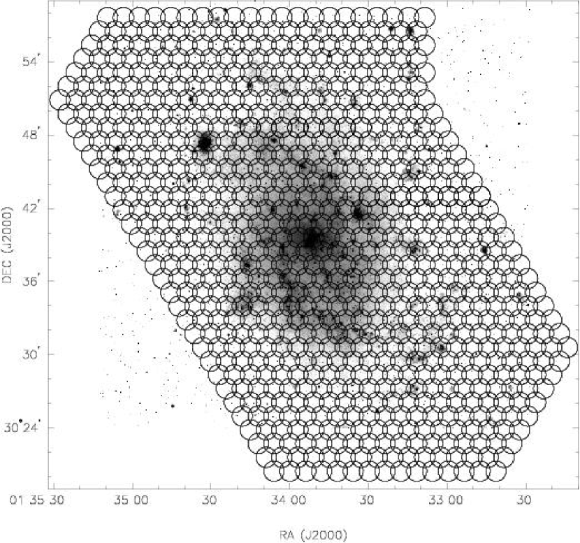
Figure 1.— Fields mapped with BIMA toward M33, overlaid on an H$\alpha$ image (Cheng et al., 1996) of the galaxy. Circles show the $100^{\prime\prime}$ FWHM primary beamwidth of the BIMA antennas at 115.27 GHz.

The CO($1\to 0$) line was observed in the upper sideband of the SIS mixers. Single sideband system temperatures, scaled to the top of the atmosphere, were typically 300 to 500 K at 115.27 GHz. The correlator covered the LSR velocity range $-414$ to $+59$ km s^-1 with 1.015 km s^-1 channel spacing, on each of the 45 baselines.

Each night we cycled through observations of about 50 grid points, using an integration time of 25 seconds per point. The slew and settle time of the telescope between integrations was 5 seconds, so a complete loop through 50 grid points required about 25 minutes. Observations of the calibrator, 0136$+$478, were interleaved with complete loops. For a typical 6-hour track, each pointing center was observed 10–12 times. With 45 baselines, this yields about 500 measurements of the source visibility across the $(u,v)$ plane, resulting in a nearly round synthesized beam with $\leq 10$% sidelobes.

A total of 45 observing tracks was obtained, with durations of a few hours to 10 hours. The total useful integration time accumulated on M33 was 132 hours, which corresponds to an average of 10.5 minutes per pointing center.

2.1. Flux Scale

For each observing track the amplitude gain of each antenna was scaled by a constant factor to obtain the correct visibility amplitude on the calibrator, 0136$+$478. The flux density of this quasar was variable over the course of the observations (2.3 Jy in 1999 September, 3.0 Jy in 2000 May, 3.7 Jy in 2000 July, and 3.4 Jy in 2000 Oct). We monitored the calibrator flux density by making a brief observation of the compact H II region W3OH once per night. The flux density of W3OH was measured to be $3.8\pm 0.2$ Jy by comparison with primary flux calibrators Mars and Uranus. All comparisons with W3OH were made using the lower sideband continuum channel of the receivers at 112 GHz, since measurements at 115 GHz are contaminated by CO emission from the extended molecular cloud associated with W3OH.

The flux densities derived for 0136$+$478 were generally reproducible to $\pm 0.2$ Jy from night to night. Allowing for possible systematic pointing errors and decorrelation by atmospheric phase fluctuations, we estimate that the final amplitude scale is uncertain by approximately $\pm 15$%.

2.2. Mapping

After calibrating the visibility data, we generated mosaiced spectral line maps using the Miriad software package. The maps were deconvolved with a CLEAN algorithm in order to remove negative bowls around the strongest sources. The synthesized beam varies slightly across the mosaic because individual subgrids have slightly different $(u,v)$ coverage. To handle this, Miriad creates a cube of synthesized beams, one for each pointing center, and interpolates among them when deconvolving the map. The maps were restored with a $13^{\prime\prime}$ Gaussian.

Most of our analysis was performed on maps with $2.03$ km s^-1 velocity resolution. These were produced by Hanning smoothing the (1.015 km s^-1 spacing) visibility spectra, then generating maps of alternate channels. The resulting channel maps are expected to be nearly statistically independent.

To evaluate the noise level across the mosaic, we computed the RMS fluctuations in the spectrum corresponding to each map pixel, omitting any channels with flux densities $S>4\sigma$. From a spectrum with 222 statistically independent channels, the noise is determined to approximately 5% accuracy. We then smoothed the map of the noise to $30^{\prime\prime}$ resolution (Figure 2). The white 99% gain contour denotes the effective outer boundary of the mosaic. Outside this contour intensities are not fully corrected for attenuation by the primary beam. For these 2 km s^-1 resolution channel maps the RMS noise level over the central half of the mosaic ranges from 0.34 Jy beam^-1 to 0.51 Jy beam^-1; the average value is 0.44 Jy beam^-1, or 0.24 K. At the worst spots near the edge of the mapped region (but inside the 99% gain contour) the noise level is sometimes as high as 0.65 Jy beam^-1.

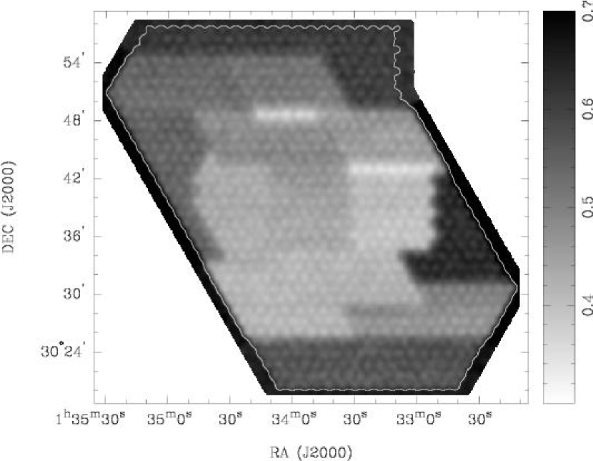
Figure 2.— RMS noise level, in Jy beam^-1, for the 2 km s^-1 resolution CO data cube. The white line near the edge of the mosaic is the 99% gain contour; outside this contour the data have not been fully corrected for the primary beam response. Within the 99% gain contour the RMS noise ranges from 0.34 to 0.65 Jy beam^-1; it is $<0.51$ Jy beam^-1 within the central half of the mosaic.

3. The GMC catalog

3.1. Identifying clouds

Because the sensitivity varies across the mosaic, we searched for molecular clouds by clipping the maps at a constant signal-to-noise ratio instead of a constant flux density threshold. The intensity data cube is converted to a signal-to-noise data cube by dividing through by the noise at each position:

$$s(x,y,\nu)=\frac{I(x,y,\nu)}{\sigma(x,y)f(\nu)},$$ (1)

where $\sigma(x,y)$ is the smoothed RMS noise map (Figure 2) and $f(\nu)$ is a frequency-dependent noise correction (Figure 3) which arises because of gain variations of $5-10\%$ across the instrumental passband. Real CO emission occupies only a few of the $\sim 20500$ independent resolution elements in each channel map, thus having little effect on the renormalization. In the normalized, or signal-to-noise, data cube the intensity is expressed as a multiple of the RMS noise at each pixel. For example, $s(x,y,v)=-3$ represents a $3\sigma$ detection of a negative peak.

Figure 3.— RMS noise as a function of $V_{\rm LSR}$, for the 2 km s^-1 resolution maps. The noise level is frequency-dependent because of gain variations across the instrumental passband. In addition, the noise is higher at the blueshifted end of the spectrum because of the rapid increase in atmospheric opacity above 115 GHz.

The maximum and minimum normalized fluxes in each velocity channel are plotted in Figure 4. CO emission is obvious in the range $-260<V_{\mathrm{LSR}}<-105$ km s^-1. A histogram of the normalized fluxes in this velocity range (Figure 5) is well-fitted by a normal distribution, apart from the wing of high signal-to-noise pixels attributable to CO detections.

Figure 4.— Maximum and minimum normalized flux (signal-to-noise ratio) vs. $V_{\rm LSR}$ for the M33 CO data cube. Maxima are indicated by the histogram, minima by open circles. The channel spacing is 2.03 km s^-1; the channels have been boxcar averaged to obtain a velocity resolution of 4.06 km s^-1. Note that this is not the CO spectrum that one would observe toward M33 with a sensitive single dish; in a large beam the bright CO peaks would be greatly diluted by their small filling factors.

Figure 5.— Histogram of normalized flux values in the signal-to-noise data cube, for 4 km s^-1 channel maps, for the velocity range $-270<V_{\mathrm{LSR}}<-100$ km s^-1. The bin size is 0.025, the total number of points is 20916120, and the smooth curve is a Gaussian of the form $y=209048\exp(-x^{2}/2)$. The positive wing is due to CO emission from molecular clouds. Since the histogram plots $\sim 12$ dependent pixels for each statistically independent beam, the scatter in the negative wing of the Gaussian is suppressed compared to if all the points were independent.

Clearly, one could comfortably accept as a CO detection any pixel with normalized flux $>5\sigma$. Unfortunately, such a simple strategy would miss much real molecular emission – Figure 5 shows a clear excess in pixels with flux $>3.5\sigma$. Since the velocity maps are nearly statistically independent, we can obtain a higher detection efficiency by searching for neighboring channels with unusually high normalized fluxes. The lowest mass molecular cloud which our survey is likely to detect is of order $2\times 10^{4}~{}M_{\sun}$. A typical Milky Way GMC with this mass has a velocity dispersion of 1.8 km s^-1 (Solomon et al., 1987), which corresponds to a FWHM linewidth of 4.2 km s^-1. Therefore, we expect that CO emission from most real clouds should appear in at least two adjacent 2 km s^-1 velocity channels. To identify molecular cloud candidates, we wrote an IDL routine to locate pairs of adjacent channels with normalized flux $>2.7\sigma$. Each pair, and all contiguous pixels with normalized flux $>2\sigma$, are assigned to a candidate molecular cloud. These pixels are then masked to avoid double counting, and a search for another candidate cloud proceeds until all pairs of adjacent $>2.7\sigma$ channels have been masked. The assignment of pixels to candidate clouds in this manner does not depend on search order but occasionally links nearby sources which could be regarded as separate clouds. Although we expect from our map statistics to find real CO emission only in the velocity range $-280<V_{\mathrm{LSR}}<-85$ km s^-1, the search was conducted over the full 450 km s^-1 range of the data cube. A total of 1600 candidate sources were identified in this way.

To evaluate the likelihood that each candidate source is real, we examine the most significant spectrum through the cloud – either the one with the highest summed significance or the one with the greatest number of adjacent channels with flux $>2\sigma$. The calculation described in Appendix A evaluates the probability $P$ that this spectrum is a noise fluctuation, i.e. that the detection is spurious. As discussed in Appendix A, the likelihood that the cloud is real is then given by $\mathrm{exp}(-NP)\sim 1-NP$, where $N$ is the number of statistically independent ways in which $n$ adjacent channels can be selected from the data cube. For the full data cube $N\sim n_{beams}\cdot n_{chans}\sim 4.5\times 10^{6}$. Note that the likelihood computation is based on a single spectrum through each cloud, not on an average over the source. This keeps the calculation simple, since adjacent spatial pixels oversample the synthesized beam and hence are not statistically independent.

Originally, we intended to catalog all candidate sources with $\lesssim 10\%$ likelihoods of being noise fluctuations. To our disappointment, however, the algorithm identified several sources which were almost certainly spurious – i.e., well outside the plausible range for CO emission – with false detection likelihoods of $<0.001$. There are several possible explanations for this inconsistency. First, there may be outliers caused by a few bad visibility measurements, perhaps from observations obtained in especially poor weather or at low elevation. Second, we may be underestimating the number $N$ of statistically independent resolution elements in the data cube. Nyquist sampling the highest spatial frequency visibility data (corresponding to antenna separations of 11.5 k$\lambda$) requires a $9^{\prime\prime}$ interval, which would imply there are $\sim 50000$ independent resolution elements in the map. We believe the actual number is close to our original estimate of 20500 because the long baseline data receive little weight in the final image. Third, there may be errors in normalizing the maps by the rms noise. Such errors are particularly likely for the frequency dependent correction (Figure 3) because there were slow changes in the passband gain over the 14 month period in which observations were made.

Because the likelihood calculation is imperfect, we use it only to rank the relative likelihoods of the candidate sources. For convenience we define a ‘likelihood measure’ as $-\ln(NP)$. Figure 6 plots this quantity vs. LSR velocity for the 1600 candidate sources. Sources with the 60 highest likelihood measures ($-\ln(NP)>13.4$) fall in the velocity range $-260<V_{\mathrm{LSR}}<-105$ km s^-1and are apparent in multiple channel maps, i.e. they are unquestionably real. As the likelihood threshold is lowered, we begin to find a few sources that probably are spurious, since they lie well outside this velocity range. At $-\ln(NP)\sim 0$ the number of obviously spurious sources rises sharply, indicating the noise floor of the data cube.

Figure 6.— Likelihood measure $\ln(NP)$ as a function of $V_{\mathrm{LSR}}$ for the 1600 cloud candidates. Large values of $-\ln(NP)$ represent the most significant clouds. Only detections within the velocity range $-280\mbox{ km s}^{-1}<V_{\mathrm{LSR}}<-85\mbox{ km s}^{-1}$ are included in the catalog. The remainder of the velocity range is used to estimate the number of false detections at a given significance. Clouds included in the main catalog are marked with large dots.

For our primary GMC catalog, we accept all cloud candidates in the velocity interval $-280<V_{\mathrm{LSR}}<-85$ km s^-1 for which $-\ln(NP)>5.83$. A total of 93 sources fit these criteria. It is straightforward to estimate the number of false detections in this catalog simply by counting the number of sources above the likelihood cutoff which lie outside the 96-channel search range. There are 3 spurious detections in the 48 channels just below the search range, and 3 spurious detections in the 48 channels just above the search range. Hence, we expect that there are of order 6 spurious detections in this catalog.

One can identify fainter sources by narrowing the search range to cover only velocities that lie within the H I emission line profile in each direction. Figure  7 shows the cloud likelihoods from Figure 6 plotted as a function of the H I–CO velocity difference. H I velocities were obtained from the Westerbork map of Deul & van der Hulst (1987), which has $12\times 24^{\prime\prime}$ resolution. For the 93 clouds in the primary catalog, the velocity difference exceeds $\sigma_{\mathrm{HI}}$ for only 5 sources, where $\sigma_{\mathrm{HI}}$ is the velocity dispersion of the H I line. The four sources with velocity differences $>2\sigma_{\mathrm{HI}}$ may be false detections.

Figure 7.— Likelihood measure vs. the CO–H I velocity difference, normalized by the H I linewidth. The most significant detections are within 3 velocity widths of the H I velocity.

Narrowing the search range to $\pm 2\sigma_{\mathrm{HI}}\sim\pm 15$ km s^-1 from the H I velocity, we identified 55 additional clouds with likelihood measure $-\ln(NP)>1.4$. Figure 8 shows these sources on a likelihood–velocity difference plot. Once again, by counting the number of (presumably) spurious sources outside the velocity search range, we estimate that there are of order 9 false detections in this catalog extension.

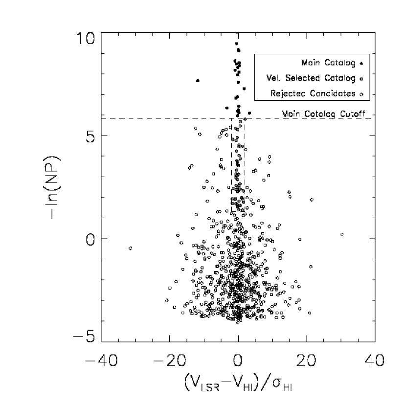
Figure 8.— The 93 clouds in the main catalog are supplemented by 55 detections selected by their proximity to the H I velocity. There is a significant overdensity of clouds near the H I velocity, reflecting the presence of real clouds that are indistinguishable from noise. Because of the narrow velocity range, we estimate that fewer than 9 of these clouds are false detections.

It is not useful to catalog individual clouds with likelihoods $-\ln(NP)<1.4$ because the number of spurious sources is quite large. Nevertheless, in Figure 8 there is an obvious overdensity of GMC candidates with $V_{\rm LSR}$ within $2\sigma_{HI}$ of $V_{\mathrm{HI}}$, and this may be used to gauge the number of cloud candidates which are falsely rejected. There are 145 candidate sources with $2<\mid V_{\mathrm{CO}}-V_{\mathrm{HI}}\mid/\sigma_{\mathrm{HI}}<4$ which are presumably spurious. One expects to find an equal number of spurious sources in the range $\mid V_{\mathrm{CO}}-V_{\mathrm{HI}}\mid/\sigma_{\mathrm{HI}}<2$. Since there are actually 205 candidate sources in this range, we estimate that roughly 60 clouds have been falsely rejected from our GMC catalog in this significance range. This result is not particularly sensitive to how we select boundaries for the overdensity band in Figure 8.

3.2. Cloud Positions, Velocities, and Masses

Figure 9 shows the most significant CO spectrum through each cloud, overplotted on the H I spectrum in the same direction. Table 1 lists the positions and properties of the 148 clouds identified in our survey, ranked by likelihood. Sources 1–93 were chosen without regard to the CO–H I velocity difference, and hence are suitable for statistical tests against the H I distribution.

Table omitted for brevity. The table is available at

http://astro.berkeley.edu/~eros/m33.table.txt

Table 1Summary of cloud parameters for HCRO observations.

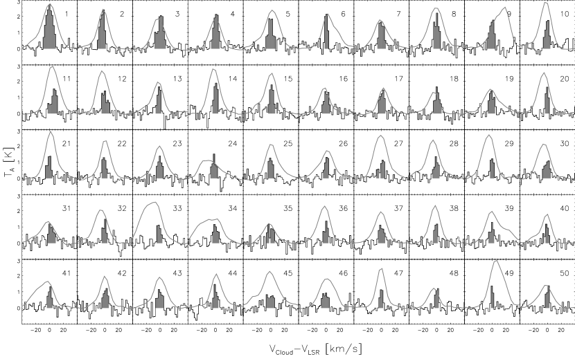
Figure 9.— Spectra for the first 50 clouds in the catalog. The channels included by the cloud identification algorithm are shaded and the grey line represents the H I line profile, scaled to have equal amplitudes for the first cloud.

The position and velocity of each cloud listed in Table 1 are intensity-weighted averages over all pixels which constitute the cloud i.e., $\bar{x}=(\sum Tx)/(\sum T)$. The velocity width is derived from the intensity-weighted second moment of the velocity distribution,

$$\Delta v_{\rm FWHM}=\left[8\,\mathrm{ln}2\,\frac{\sum T(v-\bar{v})^{2}}{\sum T}\right]^{0.5}.$$ (2)

To estimate the cloud’s mass, we convert the CO integrated intensity for each pixel to an H₂ column density $N(\mbox{H}_{2})=T(x,y,v)\Delta v\cdot X$, where $\Delta v$ is the channel velocity width, 2.032 km s^-1, and where we assume a conversion factor $X=2\times 10^{20}~{}\mbox{cm}^{-2}/(\mbox{K~{}km~{}s}^{-1})$ (Solomon et al., 1987; Strong et al., 1988; Strong & Mattox, 1996; Digel et al., 1999). The higher resolution observations presented in Paper II imply that this conversion factor is consistent with the virial masses of clouds out to radii of 4.5 kpc, despite variations in metallicity. Each pixel corresponds to a physical area $D^{2}\Delta\alpha\Delta\delta$, where $D$ is the distance to M33, 850 kpc (Lee, Freedman, & Madore, 1993, and references therein), and $\Delta\alpha$ and $\Delta\delta$ are the extent of the pixel in angle, both of which are $4^{\prime\prime}$. Thus, the total cloud mass is

$$M=\sum_{\mathrm{pixels}}1.36\cdot 2\cdot m_{H}\cdot X\cdot T_{\mathrm{pixel}}\Delta v\cdot D^{2}\Delta\alpha\Delta\delta.$$ (3)

The factor 1.36 is the mass correction for helium with a number fraction of 9% relative to hydrogen nuclei. If expressed in terms of flux density rather than brightness temperature, this is equivalent to

$$M=7.5\times 10^{3}M_{\sun}/(\mbox{Jy km s}^{-1}).$$ (4)

This is 25% lower than the conversion factor adopted by Wilson & Scoville (1990), mostly because of our choice of a lower $X$-factor.

3.3. Completeness

To gauge the completeness of the survey, we added a regular lattice of artificial test sources to the cube of channel maps and computed the fraction of them recovered by our search algorithm. Each test source was a $13^{\prime\prime}\times 13^{\prime\prime}$ Gaussian, corresponding to a GMC unresolved by our synthesized beam, with a Gaussian velocity profile. The velocity width was kept constant at 6 km s^-1 FWHM, independent of the flux density (mass) of the test source. Artificial sources were spaced by $100^{\prime\prime}$ in right ascension and declination, over the entire mosaic; and by 56.3 km s^-1 in velocity, from $-345$ to $-11$ km s^-1. Sources close to the edge of the mosaic were omitted if more than 5% of their flux lay outside the mosaic’s 99% gain contour. In total, 2625 artificial sources were added to the data cube. Source recovery tests were done with masses ranging from $3\times 10^{4}~{}M_{\sun}$ to $10^{6}~{}M_{\sun}$.

Figure 10 shows the fraction of the test sources detected as a function of the local RMS noise level. Over the full mosaic, the survey is complete to $1.5\times 10^{5}~{}M_{\sun}$. Within the central half of the mosaic, where the noise is typically $<0.5$ Jy beam^-1, we recover approximately 90% of $1\times 10^{5}~{}M_{\sun}$ clouds. Outside this region, we recover 70 — 80% of such clouds.

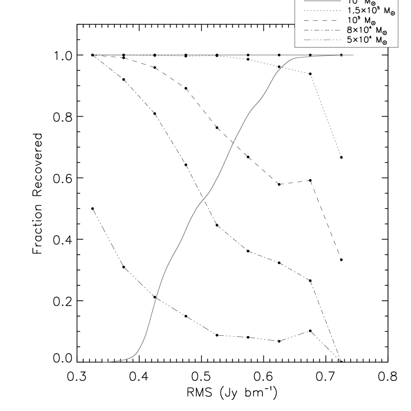
Figure 10.— Fraction of artificial clouds recovered as a function of RMS noise, for 5 cloud masses. The solid curve shows the cumulative distribution of noise in our mosaic, within the 99% gain contour. Clouds with masses $>1.5\times 10^{5}~{}M_{\sun}$ will be detected virtually anywhere in the map; most clouds with mass $>1.0\times 10^{5}~{}M_{\sun}$ will be detected within the inner half of the mosaic.

Figure 11 shows the recovered mass versus the actual mass of the test sources. Our algorithm underestimates cloud masses because it integrates the CO luminosity only over pixels inside the 2$\sigma$ brightness contour. The underestimates are particularly severe for low mass clouds, for which much of the emission is beneath below the 2$\sigma$ noise level. For clouds at the threshold of detectability, $\sim 7\times 10^{4}~{}M_{\sun}$, we recover about half the mass, whereas for clouds more massive than $2\times 10^{5}~{}M_{\sun}$, we recover more than 80%. The average correction factors from Figure 11 were applied to our catalog sources to obtain more accurate mass estimates; these are given as $M_{\mathrm{CO}}^{*}$ in column (8) of Table 1.

Figure 11.— Mass recovered as a function of test cloud mass. Inverting this relationship for masses above $5\times 10^{4}\ M_{\odot}$ determines the correction factor applied to the masses in Table 1.

3.4. Extended sources

The completeness estimates discussed above are applicable only to sources that are unresolved by the $13^{\prime\prime}$ synthesized beam, i.e. to GMCs $\ll 50$ pc in diameter. Because an aperture synthesis telescope acts as a spatial filter, attenuating low spatial frequencies, the sensitivity to larger sources is reduced. Essentially, the synthesized beam consists of a narrow positive lobe surrounded by a broad negative bowl. If one convolves an extended source brightness distribution with this beam, the negative contribution from the bowl partially cancels the positive contribution from the central lobe, reducing the observed flux density. For the BIMA D-array, the observed flux density for a $40^{\prime\prime}$ FWHM Gaussian source is about half the true flux density. Thus, our survey may not detect a group of molecular clouds with a total mass of $1\times 10^{5}~{}M_{\sun}$ spread out over a $40^{\prime\prime}$ (150 pc) region, though it is quite likely to detect a single GMC with this mass. For sources with radii comparable to the beam size, their surface brightness will be diminished relative to that of a point source by a factor of $\sim 2$. Fortunately, sources of this size are also significantly more massive ($10^{6}~{}M_{\odot}$, Paper II) than our completeness limit and would be readily detectable.

Single dish observations of M33 with the University of Arizona Steward Observatory 12-m telescope were used to estimate the total fraction of the CO flux recovered by the BIMA survey. The single dish flux calibrations were repeatable within 6%, and agreed with BIMA flux measurements of planetary and spectral line calibrators within 10%; further observational details are given in Paper II. Two sets of single dish observations were made. First, 18 positions with BIMA catalog sources were observed. For these fields the BIMA D-array maps recovered approximately 60% of the single dish CO flux. CO was detected in just 2 of the 18 off-source spectra obtained in these position-switched observations; the 16 non-detections may be used to set an upper limit of 0.3 M_☉ pc^-2 for the surface density of an extended ($R\leq 4$ kpc) uniform molecular disk. Second, we observed 15 fields to map a $7.5^{\prime}$ cut along the major axis of M33. In Figure 12 we show a composite single dish spectrum derived by shifting the spectrum for each of the 15 fields to a common velocity and averaging. The integrated flux of the of the 12 m spectrum is 1.2 K km s^-1 corresponding to $\sim$5.2 M_☉ pc^-2. This corresponds to $1.6\times 10^{7}~{}M_{\sun}$ of molecular gas in the central $7^{\prime}$ diameter of the galaxy. Wilson & Scoville (1989) measure $1.9\times 10^{7}~{}M_{\sun}$ in the same region when converted to our $X$-factor, distance, and removing their correction for source-beam coupling.

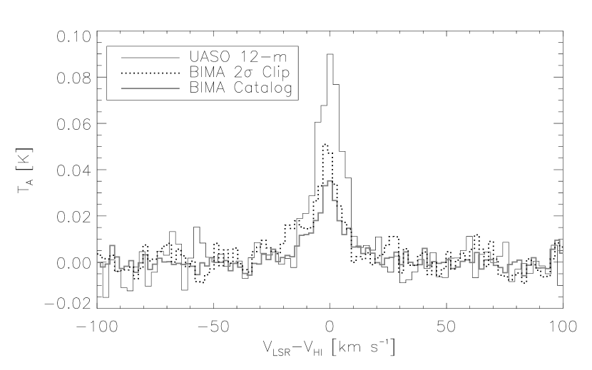
Figure 12.— A comparison of the flux selected in the D-array survey with that observed by the UASO 12-m telescope. A composite spectrum (solid line) is shown for 15 single dish fields on a $7.5^{\prime}$ cut along the major axis of M33. This is derived by shifting the spectrum for each of the fields to a common velocity and averaging. The integrated intensity of the 12 m spectrum is 1.2 K km s^-1 corresponding to $\sim$ 5.2 M_☉ pc^-2. For comparison, composite spectra are shown for BIMA data within the 12 m fields, convolved to the $54^{\prime\prime}$ FWHM 12 m beam. Two BIMA spectra were synthesized, one from the catalog source pixels only (thick line), another from the data cube clipped at 2$\sigma$ (dotted line). The BIMA catalog spectrum contains 43% of the single dish flux, the clipped spectrum, 54%.

For comparison between the 12 m and the interferometer, we show composite spectra made from BIMA data within the 12 m fields, convolved to the $54^{\prime\prime}$ FWHM 12 m beam, sampled at the centers of the 12 m beams, and averaged together in a fashion identical to the 12 m spectra. Two BIMA spectra were synthesized, one from the catalog source pixels only (thick line), another from the data cube clipped at 2$\sigma$ (dotted line). The BIMA catalog spectrum contains 43% of the single dish flux, the clipped spectrum, 54%. In Paper II we argue that most of the missing flux is attributable to complexes of undetected low mass clouds associated with catalog sources.

We can estimate the total molecular mass of M33 from the major axis cut. The integrated single dish molecular mass in this $7.5^{\prime}$ long strip is $2.8\times 10^{6}~{}M_{\sun}$. The corresponding BIMA mass, considering only cataloged clouds with masses greater than $1.5\times 10^{5}~{}M_{\sun}$, the completeness limit for our survey, is $9.2\times 10^{5}$ M_☉, 33% of the single dish mass. In this computation we have weighted the cloud masses by the appropriate 12-m beam attenuation factors. The total (corrected) mass in the catalog is $2.3\times 10^{7}~{}M_{\sun}$, of which 1.5$\times 10^{7}~{}M_{\sun}$ is from clouds more massive than the completeness limit. If the GMC mass spectrum in the central cut is similar to that for the galaxy as a whole, then we infer that the total molecular mass is 3 times this value, or 4.5$\times 10^{7}~{}M_{\sun}$.

3.5. Comparison with Wilson and Scoville 1990

Wilson & Scoville (1990, hereafter WS90) used the Owens Valley array to map 19 fields in the nucleus of M33 with $7^{\prime\prime}$ resolution, identifying 38 molecular clouds. Figure 13 is an overlay of the WS90 fields on the central $10^{\prime}\times 10^{\prime}$ section of the BIMA survey. Red contours show the outer boundary of clouds identified in the BIMA survey; solid circles mark locations of clouds cataloged by WS90. Frequently, a BIMA cloud corresponds to two or more WS clouds – for example, the complex WS1-WS5 at the center of the galaxy is classified as one cloud in our survey because these sources are connected by low-level emission and lower BIMA resolution blends these clouds together. The BIMA survey detects all of the WS90 clouds with masses $>2\times 10^{5}M_{\odot}$.

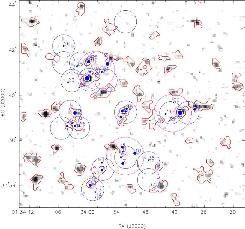
Figure 13.— Comparison of BIMA and WS90 molecular clouds in M33. The map covers the central $10^{\prime}\times 10^{\prime}$ region of M33. The gray scale shows a BIMA D-array image generated by masking out all emission $<2\sigma$ in individual 2.03 km s^-1channel maps, then integrating over the velocity interval $-240<$ $V_{\rm LSR}$$<-128$ km s^-1. Red contours show the outer boundaries of BIMA clouds determined by our search algorithm. Open blue circles show the 19 fields mapped by WS90; sources cataloged by WS90 are shown as filled blue circles, with area proportional to mass. Magenta circles indicate the 3 fields mapped in the BIMA C-array, as described in the text.

To examine a few of our clouds more closely, and to investigate discrepancies between our catalog and the WS90 catalog, we obtained higher resolution BIMA observations of the three fields shown by dashed circles in Figure 13. These fields were observed on 3 nights in 2000 July with the array in its “C” configuration. The integration time was approximately 6 hours per field. The C-array observations were calibrated and combined with the D-array data to generate maps with a $6.5^{\prime\prime}$ synthesized beam. The RMS noise level in each 2.03 km s^-1 channel map was 0.15 Jy beam^-1, approximately 0.32 K, comparable to that of WS90. The C$+$D-array maps are compared with the D-array survey images in Figure 14.

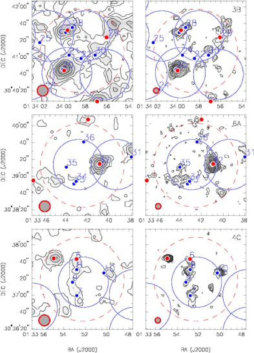
Figure 14.— Comparison of BIMA D-array and C$+$D-array maps of 3 fields. BIMA catalog sources are shown by red dots, WS90 sources by blue dots.

Generally there is good agreement between sources in our C+D array images and the WS90 positions, although we fail to confirm some of the less massive WS90 clouds (e.g., WS21, WS22, WS36). One can find several examples showing how the D-array survey blends WS sources (e.g., WS27 and WS28 = catalog source no. 17; WS6 + WS8 = catalog source no. 74).

Figure 15 compares the masses of GMCs which can be clearly identified in both data sets. As indicated by the dashed line, the BIMA masses are expected to be systematically lower by 25% because we used a lower conversion factor from flux density to mass. Generally the BIMA and WS90 masses are in reasonable agreement, although there is a good deal of scatter in the ratio, probably because of the difficulty in establishing the outer boundaries of clouds.

Figure 15.— Comparison of GMC masses from the BIMA D-array survey and the WS90 survey, for cases where the same source clearly is detected by both surveys. The dotted line shows the expected slope, given the different mass conversion factors used in the two surveys.

Small clouds detected by the C-array observations are not included in our survey catalog (Table 1) but a further analysis of these clouds is included in Paper II.

4. Cloud Properties

4.1. GMC Mass Spectrum

Histograms of the mass distribution of GMCs in our catalog are presented on a log-log scale in Figure 16. The dashed line histogram is the observed spectrum of GMC masses uncorrected for signal beneath the $2\sigma$ clipping level, as described in §3.3. The solid line histogram is the spectrum of corrected masses. A power law of the form

$$\frac{dN}{dM}=K\left(\frac{M}{M_{\sun}}\right)^{-\alpha}$$

was fit to the mass bins for which the catalog is complete ($M>1.5\times 10^{5}~{}M_{\sun}$). The observed and corrected mass distributions are well fit with similar indices ($\alpha=2.6\pm 0.3$) but different normalization constants ($K=1.2$ vs. $1.8\times 10^{10}M^{-1}_{\sun}$).

Figure 16.— The mass distribution $dN/dM$ of the GMC catalog. Solid line histogram shows the distribution of masses corrected for emission profile truncation at 2$\sigma$. (Refer to Figure 11.) Dotted line histogram shows the distribution of uncorrected masses. The histograms have been accumulated into half-octave mass bins ($\Delta\log M=0.5\log_{10}2$), where the zero reference is $10^{5}~{}M_{\sun}$ on the abscissa and $10^{-5}~{}M^{-1}_{\sun}$ on the ordinate. Power law fits show that the mass correction has little effect on the slope of the distribution for $M>1.5\times 10^{5}~{}M_{\sun}$, but increases the normalization coefficient 30%.

For a mass spectrum with $\alpha<2$, most of the integrated mass resides in the most massive clouds. For a mass spectrum with $\alpha>2$, most of the mass is in the least massive clouds, and the total mass diverges when extended to arbitrarily small mass. Hence, for M33 there must be either a lower mass limit for molecular clouds or a break in the distribution where $\alpha$ changes with decreasing cloud mass to less than 2. If the integrated mass

$$M_{total}=\int_{low~{}limit}^{\infty}M~{}dN=\int_{low~{}limit}^{\infty}M\left(\frac{dN}{dM}\right)dM$$ (5)

is distributed according to

$$\frac{dN}{dM}=1.8\times 10^{10}\left(\frac{M}{M_{\sun}}~{}\right)^{-2.6}~{}[M^{-1}_{\sun}]$$ (6)

we compute a strict lower mass limit $M_{L}$ of $4\times 10^{4}~{}M_{\sun}$ for $\alpha=2.6$ and $M_{total}=4.5\times 10^{7}\ M_{\odot}$. More likely, there is a ”turnover” mass, where the mass spectrum becomes flatter than 2. Since we can put a firm lower limit on the cutoff mass of $4\times 10^{4}~{}M_{\sun}$ and an upper limit of $10^{5}~{}M_{\sun}$, where the measured mass distribution is nearly complete, the turnover mass of GMCs is $\sim~{}7\times 10^{4}~{}M_{\sun}$ with an uncertainty of $3\times 10^{4}~{}M_{\sun}$. This turnover represents a “characteristic” mass for the molecular clouds in M33 that any theory of GMC formation must be able to reproduce, given the physical conditions in M33.

The highest mass we measure for a GMC in M33 is $7.3\times 10^{5}~{}M_{\sun}$; there are two GMCs with this mass. Neither is close to the galactic center nor to an especially bright H II region. In total, we find five GMCs more massive than the highest mass cloud ($4\times 10^{5}~{}M_{\sun}$) reported by Wilson & Scoville (1990). Moreover, they find a lower value of $\alpha$ (1.7), which may have resulted from preferentially targeting massive clouds by observing CO-bright single dish fields.

4.1.1 M33, Milky Way, and the LMC

Over a similar mass range, the power law distribution of M33 is steeper than that of the Milky Way (1.6, Solomon et al. 1987; 1.9, Heyer, Carpenter, & Snell 2001). If M33 were as massive as the Milky Way, the normalization constant of its power law distribution would be $3.6\times 10^{11}~{}M^{-1}_{\sun}$ and $({dN}/{dM})\Delta M\sim~{}1.0$ at $1.0\times 10^{6}~{}M_{\sun}$. In contrast, the Milky Way is estimated to have more than 100 GMCs with $M>1.8\times 10^{6}~{}M_{\sun}$ Dame et al. (1986). We conclude that M33, even though it has many bright H II regions (Israel & van der Kruit, 1974), has significantly fewer massive GMCs. As we infer in $\S\ref{ha_compare}$, the majority of H II regions must be (1) fueled by molecular clouds below our completeness threshold or (2) capable of efficiently dispersing their parent GMC complexes (Hartmann, Ballesteros-Paredes, & Bergin, 2001). Extrapolating the observed power law index to a cut-off $3.0\times 10^{4}~{}M_{\sun}$, we find $\int(dN/dM)\ dM~{}\sim~{}2000$. This is a sufficient number of molecular clouds to match approximately the observed number of H II regions.

The NANTEN survey of CO in the LMC revealed 168 GMCs (Fukui et al., 2001). The cloud sample has a mass range and completeness limit similar to the BIMA survey. The mass spectrum of GMCs in the LMC has an index of  1.9, similar to that of the outer Milky Way (Heyer, Carpenter, & Snell, 2001), indicating that most of the mass resides in high mass clouds. The physical meaning of the difference between the mass indices of the LMC and M33 is unclear. However, as in M33, molecular clouds in the LMC appear to be tightly correlated with H I overdensities (Mizuno et al., 2001), and H I filaments underlie bright complexes of GMCs (§5.3). Hence, we expect the details of GMC formation to be at least somewhat similar for M33 and the LMC.

4.1.2 Cloud Masses versus Radius

Figure 17 shows the distribution of catalog GMC masses as a function of galactocentric distance. The distribution of clouds with masses greater than our completeness limit (1.5$\times 10^{5}~{}M_{\sun}$) appears to cut off abruptly beyond 4 kpc. For $R_{gal}>4.5$ kpc, we detect only a few low mass clouds despite considerable reserves of H I here (§5.1). However, higher sensitivity measurements are required to determine if we are indeed observing a sharp edge to the molecular disk or a shift to the production of predominantly low mass clouds. For $R_{gal}<4.5$ kpc, the mass distribution appears more or less constant to the eye; i.e. the apparent density of points in Figure 17 appears constant with $R$ for a given mass.

Figure 17.— Catalog GMC mass ($M^{*}_{\mathrm{CO}}$) as a function of radius. No high mass clouds are found beyond 4.5 kpc. Within this boundary the mass distribution is roughly independent of radius. Survey coverage is complete to 5.2 kpc and more than 50% complete between 5.2 kpc and 8 kpc. Accounting for incomplete coverage should, at most, double the number of clouds seen in this range.

In a more quantitative comparison, we looked for spatial variations in the GMC mass spectrum by partitioning our catalog into an inner and outer disk sample, each containing an equal mass of molecular gas in catalog GMCs. The radius at which this occurs is 2.0 kpc. This coarse radial binning assures adequate statistics for $M>1.5\times 10^{5}~{}M_{\sun}$ in two distinct cloud populations. Power law fits give $\alpha=2.8\pm 0.3$ for the inner disk and $\alpha=2.4\pm 0.3$ for the outer disk. A 2-sided K-S test shows that the two cloud samples are drawn from the same population with a 9% likelihood. Though there is some evidence for a difference in the mass distribution, it is only marginally significant.

5. Spatial Comparison of GMCs, H I Structure, and H II Regions

5.1. Radial Profiles and Star Formation Rates

For galactic radii $R<7$ kpc, we derived the azimuthally averaged mass surface density from our catalog GMCs. The results are presented in Figure 18, along with the surface density of H I mass and H$\alpha$ flux. Points represent averages within deprojected radial bins of $\Delta R$ = 0.25 kpc. The H I data are from Corbelli & Salucci (2000) and the H$\alpha$ data are derived from the optical H II region catalogs compiled by Hodge, et al. (1999). All three components of the ISM are well fit by an exponential disk $\Sigma(R)=\Sigma_{0}\exp(-R/R_{0})$. Only the fit to the molecular data is shown (dot-dash line) in the figure. The molecular surface density $\Sigma_{\mathrm{H2}}$ (squares) declines exponentially with $R_{0}=1.4\pm 0.1$ kpc, from a peak mass surface density $2.15\ M_{\sun}\mbox{ pc}^{-2}$. Corbelli (2003) obtained a total molecular gas mass of $2\times 10^{8}M_{\odot}$ from an FCRAO survey. Accounting for the difference in $X$ factors (Corbelli (2003) used $2.8\times 10^{20}\mbox{cm}^{-2}/(\mbox{K~{}km~{}s}^{-1})$), her reported mass is 3 times the value we derive. The surface mass densities in the central region are comparable, but the scale length in Corbelli (2003) is 2.5 kpc, resulting in a significantly larger integrated mass. The reason for the difference in the derived scale lengths is unclear and merits further investigation. The H I surface brightness (dashed line) is nearly flat for $R<6$ kpc with a scale length $10^{+8}_{-2}$ kpc and a peak surface density of $9.5\ M_{\sun}\mbox{ pc}^{-2}$. H$\alpha$ surface brightness (solid line) has a scale length of $1.7\pm 0.2$ kpc and a peak surface brightness of $1.2\times 10^{32}~{}\mbox{ergs s}^{-1}~{}\mbox{pc}^{-2}$, corresponding to a star formation rate of 9.5 $\times 10^{-10}M_{\sun}\ \mbox{yr}^{-1}\mbox{ pc}^{-2}$.

Figure 18.— The (deprojected) radial profiles of the molecular, atomic, and ionized media. All three are well fit by an exponential disk and can be characterized by a peak value and a radial scale length. Only the fit to the molecular data is shown (dot-dash line). Points represent averages within deprojected radial bins with $\Delta R$ = 0.5 kpc. The molecular data (squares) are well fit by an exponential disk for $R<4$ kpc with a scale length of $1.4\pm 0.1$ kpc and a peak mass surface density, $\Sigma_{\mathrm{H2}}=2.15\ M_{\sun}\ \mbox{pc}^{-2}$; $\Sigma_{\mathrm{H2}}$ drops sharply at $R=4$ kpc. The H I surface brightness (dashed line) is nearly constant for $R<6$ kpc with a scale length $10.6\pm 2$ kpc and a peak surface density of $\Sigma_{\mathrm{HI}}(R=0)=9.5\ M_{\sun}\mbox{pc}^{-2}$ H$\alpha$ surface brightness (solid line) has a scale length of $1.7\pm 0.2$ kpc and a peak surface brightness of $1.2\times 10^{32}\mbox{ergs s}^{-1}\mbox{ pc}^{-2}$.

Kennicutt (1989,1998) has argued that there is a simple empirical relation between the SFR and the surface density of gas, $\Sigma_{gas}$, which can be parameterized by a power law SFR $\propto(\Sigma_{gas})^{n}$. The SFR is most conveniently calculated by scaling the H$\alpha$ line emission, powered by OB stars. Similar scale lengths for H$\alpha$ and $\Sigma_{\mathrm{H2}}$ in M33 imply $n=0.9\pm 0.1$, consistent with a constant SFR per unit molecular mass. Similarly, Wong & Blitz (2002) find for a sample of 7 normal spiral galaxies that $\Sigma_{\mathrm{SFR}}$ strongly correlates with $\Sigma_{\mathrm{H2}}$ only, where the power law index $n\sim$ 0.8 — 1.4. Integrating $L_{\mathrm{H\alpha}}$ for the catalog of Hodge, et al. (1999) and using Equation 2 of Kennicutt (1998), we compute a star formation rate of 0.24 $M_{\sun}~{}\mbox{yr}^{-1}$ and a molecular gas depletion time of $1.9\times 10^{8}$ yr for M33. This value is a factor of 1.5 – 4 smaller than the depletion times quoted in Wilson, Scoville, & Rice (1991) who consider individual molecule-rich complexes as opposed to the galaxy as a whole. Our results, along with those of Wong & Blitz (2002), are inconsistent with those of Kennicutt (1989), who finds for disk-averaged observables that the SFR correlates more strongly with the surface density of either H I or H I$+\mathrm{H_{2}}$ than with that of molecular gas alone.

5.2. Circular and Radial Motions of Molecular and Atomic Hydrogen

We derived the rotation curve for GMCs cataloged independently of $V_{\mathrm{HI}}$ (catalog sources 1 – 93) and for the H I emission along the same line-of-sight from the Westerbork data cube (Deul & van der Hulst, 1987). The observed source positions $(x,y)$ were deprojected onto the plane of the galaxy assuming a P.A. of $\sim 21^{\circ}$ and an inclination angle of $\sim 51^{\circ}$. These values were varied slightly with galactic radius in accordance with the tilted ring model of Corbelli & Salucci (2000). The rotation center was assumed to coincide with the optical center. At the deprojected positions the rotational velocity

$$v_{rot}(R)=\frac{V_{los}(x,y)-V_{sys}}{\sin i\cos\theta},$$ (7)

where $\theta$ is the azimuthal angle of the source measured in the plane of the galaxy from the the major axis. Sources within $45^{\circ}$ of the minor axis were not included because of the large correction to ($V_{los}(x,y)-V_{sys}$).

Figure 19 shows the circular velocities for catalog GMCs, averaged in 250 pc bins. The median CO rotation curve (open squares) closely matches the H I rotation curve determined by Corbelli & Salucci (2000) from Westerbork data. The dispersion of GMCs about the H I rotation curve varies between 7.5 and 9.0 km s^-1  for $R<4~{}$ kpc. There is no apparent trend in the dispersion with galactic radius. These values are comparable to Milky Way values after streaming in the Galaxy is taken into account.

Figure 19.— Radial profiles of circular and radial motion of primary catalog GMCs, averaged over deprojected annuli of $\Delta R=250$ pc. Model rotation curve of H I also shown (dash). To measure the radial motions, only clouds within $30^{\circ}$ of the minor axis were included.

Figure 19 also shows the CO radial velocities

$$v_{rad}(R)=\frac{V_{los}(x,y)-V_{sys}}{\sin i\sin\theta},$$ (8)

including only sources within $\Delta\theta<30^{\circ}$ of the minor axis. We find little evidence for large scale radial (non-circular) motions in M33 in agreement with Deul & van der Hulst (1987).

5.3. Spatial Comparison of GMC Distribution with H I Filaments

An extraordinary spatial correspondence between GMCs and the distribution of atomic hydrogen is shown in Figure 20. The halftone image is the H I  brightness distribution, derived by integrating the Westerbork data cube (Deul & van der Hulst, 1987); the resolution of the Westerbork map is $24^{\prime\prime}\times 24^{\prime\prime}$, comparable to the BIMA data. The H I  distribution is dominated by bright, narrow filaments in an extended disk. The dark circles mark the positions of the catalog GMCs; cloud masses are proportional to circle areas. Figure 21 shows that nearly all GMCs are found in regions of H I overdensity, but there is no correlation between the magnitude of the overdensity and the cloud mass. Apparently, the amount of ambient H I is independent of the mass of the GMC that forms from it. The correspondence between GMCs and filaments persists down to smaller scales in the central region where the H I brightness map has less dynamic range. The association with the filaments is even more pronounced in the high resolution H I maps of M33 made at the VLA (Thilker, private communication). The average H I mass located within 150 pc of our catalog sources is $5\times 10^{5}~{}M_{\sun}$, indicating an ample local supply of atomic hydrogen from which observed GMCs could have condensed.

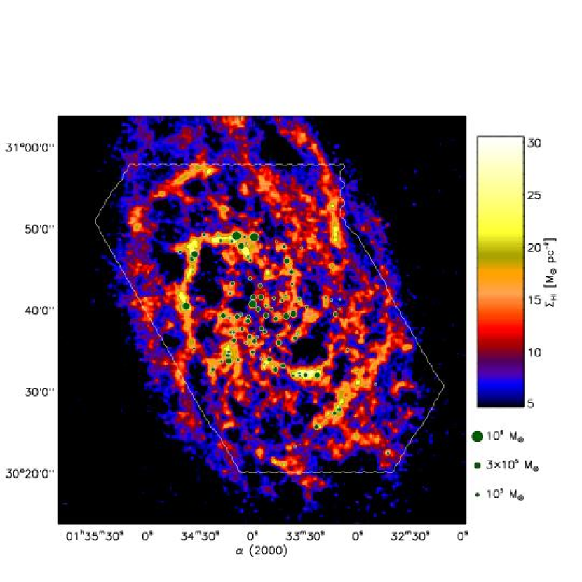
Figure 20.— Color image of H I 21 cm emission from Deul & van der Hulst (1987) with catalog sources overlayed. All molecular clouds lie in regions of H I overdensity. The area of the molecular cloud has been scaled to represent the relative masses of the clouds. The coincidence of molecular clouds with H I overdensity is evidence that clouds form out of the atomic gas.

Figure 21.— Plot of the mass of a GMC against the H I overdensity at the galactic radius of the cloud. The overdensity is defined as the H I surface density observed at the position of the cloud divided by the azimuthally averaged H I surface density found at that radius. The plot shows that there is no relation between these two quantities. Note that a few low mass clouds are found in regions of H I underdensities. These may be among the clouds in the catalog that are not real.

In Figure 22, we see that GMCs form from H I with an column density threshold of $\sim 5\times 10^{20}~{}\mbox{cm}^{-2}$, which is comparable to the mean H I column density in the H$\alpha$ disk (dashed histogram). The shaded histogram indicates pixels with associated CO emission. The solid line shows all WSRT pixels Deul & van der Hulst (1987). The threshold value is similar to that found by Savage, et al. (1977) and Blitz, Bazell & Desert (1990) in the solar vicinity, and is indicated in Figure 22. Moreover, the H I shows an upper limit in column density of $\sim 3\times 10^{21}\mbox{ cm}^{-2},~{}A_{V}\sim 3$, often at positions associated with molecular gas. This suggests that the atomic gas is providing shielding for the molecular gas, but higher column densities result in more gas in the molecular state.

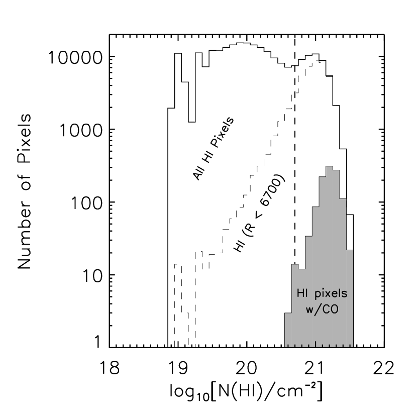
Figure 22.— Histogram of H I column densities in the WSRT map of M33 (Deul & van der Hulst, 1987). The solid histogram shows the column densities for pixels through the entire map. The dashed histogram represents pixels within 6.7 kpc of the center (the H$\alpha$ disk). The shaded histogram represents pixels associated with CO emission, that is pixels within the 2$\sigma$ boundaries of our 148 cataloged clouds. The dotted vertical line at $5\times 10^{20}\mbox{ cm}^{-2}$ is the threshold column density for molecule formation in the solar vicinity (Savage, et al., 1977).

The close association between GMCs and H I filaments can be used to set an upper limit on the GMC lifetimes. The RMS difference between the CO and H I velocity centroids is 8 km s^-1, calculated from clouds 1–93, which were selected independent of the H I velocity. The typical width of an H I filament in the Deul & van der Hulst (1987) map is $\sim 200$ pc. If cloud lifetimes were significantly longer than 10–20 Myr, clouds would drift off the filaments, destroying the observed association.

5.4. Implications for GMC Formation

Elmegreen (1990) reviews many theories of GMC formation, including the agglomeration of small molecular clouds (Scoville & Hersh, 1979). However, there can be little doubt that the GMCs in M33 form out of the atomic gas. If instead the atomic gas resulted from the dissociation of molecular gas, the H I would appear as discrete envelopes around the GMCs rather than as filaments, and there would little atomic gas beyond the apparent edge of the molecular disk at $R=4$ kpc. Neither of these features are seen. In addition, there is significantly more atomic gas ($\sim$ a factor of 5) in the filaments than can be associated with discrete envelopes around GMCs and $<15\%$ of this mass can be attributed to photodissociation (Wilson & Scoville, 1991). Furthermore, if GMCs formed by the collisional agglomeration of smaller molecular clouds, the growth time would be comparable to the collision time. This is roughly equal to the collision time of the catalog clouds, which is $2\times 10^{9}$ years based on 140 GMCs inside a radius of 4 kpc, an H₂ half thickness of 100 pc and a cloud-cloud velocity dispersion of 10 km s^-1. Since the number density of clouds scales roughly as $1/M_{cloud}$ and the geometric cross section scales as $M_{cloud}$ (owing to GMCs having a constant surface density, see Paper II), this collision time is independent of mass and characterizes the growth time for all self-gravitating clouds. Gravitation effects do not significantly enhance the collision cross section (Scoville & Hersh, 1979; Blitz & Shu, 1980). Additionally, Paper II sets an upper limit for the diffuse H₂ surface density of 0.3 M_☉ pc^-2. Forming a $10^{5}$ $M_{\sun}$ GMC from a diffuse molecular component at this surface density would require almost 10⁸ yr to accumulate material from a 300 pc radius region, provided that the gas velocity dispersion could be converted into ordered motion. Both times are considerably longer than the lifetimes of the GMCs ($\sim 2\times 10^{7}$ yr) based on their association with the H I filaments.

It appears that the process of GMC formation in M33 is first and foremost a process of H I filament formation. While a high H I column density is a necessary condition for the formation of a GMC, it clearly is not a sufficient condition, since there are many positions with high H I column densities but no observed CO emission (Figure 22). The filamentary structures extend out to the $R=8$ kpc edge of the H I map, well beyond the radius where GMCs are observed, with no significant change in character at the edge of the molecular disk. It appears that some physical parameter, which evidently is a function of galactic radius, determines what fraction of the atomic gas in a filament is converted into molecules. A likely candidate is hydrostatic pressure in the disk, a hypothesis that will be investigated in a subsequent paper.

5.5. Are GMCs and H I Holes Physically Linked?

Expanding shells in the interstellar medium may play an important role in the dynamics of the neutral gas, transmitting both mechanical and radiant energy at their boundaries (McKee & Ostriker, 1977). Deul & den Hartog (1990, DdH) cataloged 148 holes (underdensities) in the H I distribution of M33. Ninety-three of the holes (Types 2 and 3 in DdH) show the kinematic evidence of expansion in the Westerbork channel maps. These holes cover $<20\%$ of the neutral disk area. DdH find that many of the compact holes have OB associations inside and conclude that many such holes have been excavated by massive star formation activity. While DdH also allow for the possibility that holes are formed by the local collapse of H I to form GMCs, our CO survey shows that this is unlikely, since nearly all GMCs are outside the holes. In this section we consider evidence of a physical connection between GMCs and the H I shells.

There is, in fact, a tendency for the catalog GMCs to be spatially clustered around the DdH H I holes. We quantified this effect by measuring the fraction of GMCs located within annuli of width $\Delta R$ bounding the holes, and comparing this to the fraction expected if the GMCs and holes are uncorrelated. We restricted the analysis to holes with diameters less than 400 pc because these are more likely to have been created by high mass star formation. The results are shown in Figure 23. We find a significant correlation between GMCs and H I hole edges for $\Delta R$ between 60 and 300 pc, most significantly for $\Delta R$ = 150 pc (binomial probability $P_{rand}\sim 10^{-3}$). The large separation (150 pc) between hole edges and GMCs suggests, however, that expanding shells do not directly trigger formation of the GMCs. Figure 24 plots the GMCs (boundaries defined by the 2$\sigma$ clipping levels) and the 150 pc annuli (shaded) around the (compact) hole edges. This figure shows that there is no significant CO emission inside the DdH holes.

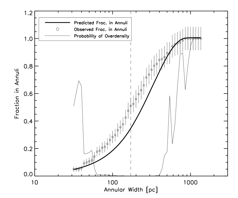
Figure 23.— Positional correlation of catalog GMCs with  H I holes cataloged by Deul & den Hartog (1990). Open circle denote the fraction of clouds which overlap an annulus of width $\Delta R$ bounding some hole with diameter $<$ 400 pc. The thick curve denotes the fraction of overlap expected for randomly distributed clouds. The thin curve is the binomial probability for the observed deviation, which is $<$ 0.05 for annular widths of 60 — 300 pc. The minimum probability 0.003, marked by the dashed line, occurs at an annular width of 150 pc.

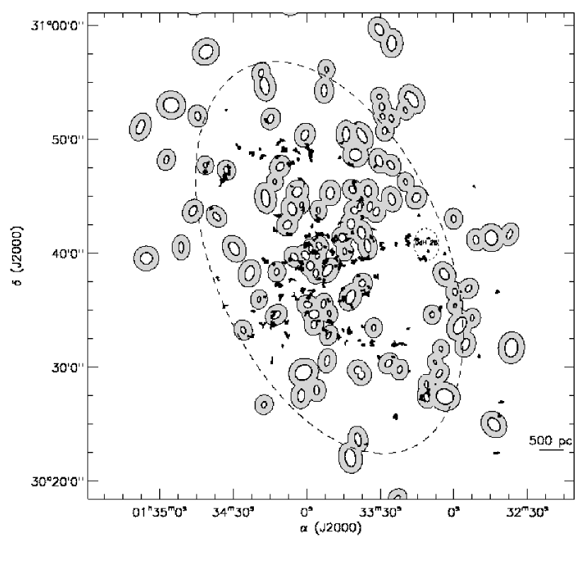
Figure 24.— HI holes and associated GMCs. Shown are 2$\sigma$ boundaries (filled) of catalog GMCs and 150 pc annuli (shaded areas) around DdH hole edges. From this figure it can be seen that no significant CO emission extends into the DdH holes. The large separation (150 pc) between hole edges and GMCs suggests that expanding shells do not directly trigger formation of the catalog GMCs. An extraordinary hole-GMC association (labeled DdH 28) may be evidence of a high velocity cloud impacting the H I disk.

Since essentially all GMCs are on filaments but not all GMCs are at the edges of holes, we conclude that the filamentary structure is more fundamental to GMC formation than the action of expanding shells. These shells may create filamentary structure on small scales, especially in the presence of turbulence (e.g. Hartmann, Ballesteros-Paredes, & Bergin, 2001), but are unlikely to produce the largest filaments. The energies required to evacuate the large holes defining these filaments are $\geq 10^{53}$ ergs (see e.g. DdH). Such energies would leave bright stellar remnants at the centers of the large holes, which are not generally observed. In addition, these holes would be sheared apart on time scales of $2\times 10^{7}$ years by differential galactic rotation unless they were stabilized by some process. Thus some organizing principle other than stellar feedback seems to be responsible for much of the filamentary H I structure, and ultimately, for GMC formation in M33. One possibility is MHD instabilities in a self-gravitating, shearing disk (Elmegreen, 1987; Kim, Ostriker, & Stone, 2002).

Although nearly all GMCs are outside holes on filaments of H I, an exception is DdH 28 (Figure 24). The catalog GMCs in this hole may result from a high velocity cloud (HVC) colliding with the H I disk. This scenario for hole creation was first elaborated by Tenorio-Tagle (1981). GMCs 66 and 88 have velocities blue-shifted relative to local H I by 72 and 24 km s^-1, respectively. The formation of GMCs 40, 51, 54, 123, and 133 at the edge of the hole – all blueshifted relative to local H I– may have been triggered by this collision as well. The combined kinetic energy of these clouds ($1.4\times 10^{52}$ ergs) could have been supplied by an atomic HVC. Alternatively, GMCs in DdH 28 may have formed on the front surface of neutral shells. That is, they may be similar to the Orion A and B molecular clouds, which appear to have formed from gas lifted 140 pc out of the plane of the Milky Way by stellar winds (Dame, Hartmann, & Thaddeus, 2001; Hartmann, Ballesteros-Paredes, & Bergin, 2001).

5.6. Spatial Comparison of GMC Distribution with H II Regions

Figure 25 compares the locations of GMCs with H$\alpha$ emission, showing that some GMCs follow the weak H$\alpha$ spiral arms of M33. Molecular clouds in the overlay are represented by filled circles with area proportional to mass; the underlying halftone is a CCD image from Cheng et al. (1996). Most of the H$\alpha$ flux comes from H II regions, which are cataloged in Boulesteix et al. (1974), Wyder, Hodge, & Skelton (1997), and Hodge, et al. (1999). As shown in §5.1, the radial profiles of CO flux and H II region flux have comparable scale lengths; however, not all H II regions are associated with GMCs. In fact, there are over 20 times as many H II regions as catalog GMCs, and many of the H II regions are far from detected clouds. Since our GMC catalog has a lower dynamic range than the H II region catalog, it’s possible that low mass GMCs are associated with most of these “orphan” H II regions; §4.1 argues that there could be $\sim$ 2000 molecular clouds in M33, comparable to the number of H II regions. Alternatively, H II regions may rapidly dissipate molecular clouds, accounting for the discrepancy in numbers (Hartmann, Ballesteros-Paredes, & Bergin, 2001).

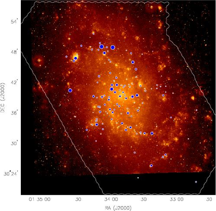
Figure 25.— Location of GMCs plotted with blue circles on the H$\alpha$ image of Cheng et al. (1996). The area of circles is proportional to the molecular mass.

We calculate the fraction of the H$\alpha$ flux that originates from H II regions that spatially overlap catalog GMCs. Using the positions and radii of H II regions from the combined catalogs (Boulesteix et al., 1974; Wyder, Hodge, & Skelton, 1997; Hodge, et al., 1999), we find that 40% of the H$\alpha$ flux originates from H II regions which are tangent to, or contain, catalog GMCs. If the remaining $2.2\times 10^{7}\ M_{\odot}$ of molecular gas (§3.4) produced a proportional amount of H$\alpha$ flux, at least 80% of the emission would arise from H II regions associated with GMCs.

One may also ask what fraction of the GMCs are actively forming stars. Figure 26 shows the positional correlation of catalog GMCs with H II regions (circles). We counted the fraction of GMCs that have at least one H II region within distance $\Delta r$. The thin curve is the fraction expected from random association (see Appendix B). There is a statistically significant clustering of GMCs and H II regions out to a separation of 150 pc. As many as 100 GMCs (67%) are apparently forming massive stars – that is, their centroid position is within 50 pc of some H II region. This is a similar fraction of association as found in a more limited study by Wilson & Scoville (1991). Of the remaining GMCs, we estimate that only a few contain obscured H$\alpha$ sources. From our correlation curve, there are only 7 H II regions coincident with a GMC position ($\Delta r\leq 10$ pc). By symmetry, we expect that only $\sim 7$ catalog GMCs are obscuring signs of massive star formation.

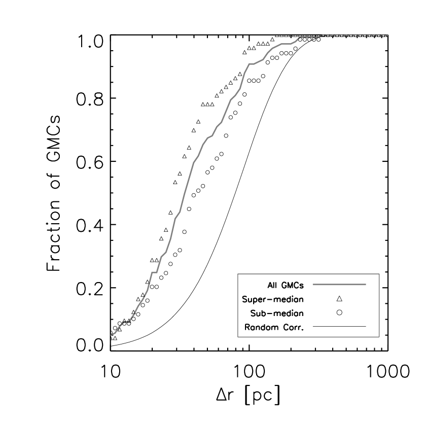
Figure 26.— Figure 26 shows the positional correlation of catalog GMCs with H II regions. The H II region positions are from the combined catalogs of Boulesteix et al. (1974), Wyder, Hodge, & Skelton (1997), and Hodge, et al. (1999). We measured the fraction of GMCs with at least one H II region within a separation $\Delta r$. The thin curve is the fraction expected from random association. There is statistically significant clustering of GMCs and H II regions out to a separation of 150 pc. As many as 100 GMCs (67 %) are apparently forming massive stars – that is, their centroid position is within 50 pc of some H II region. 85% of the higher mass GMCs (triangles) are within 50 pc of H II regions versus 55% of the lower mass GMCs (circles). This result is consistent with a shorter quiescent time for higher mass clouds.

Winds and ionizing radiation from massive stars destroy molecular clouds. Since at least 2/3 of our sources are associated with H II regions, we infer that GMCs spend less than 1/3 of their life in a quiescent phase prior to the onset of massive star formation. The fraction of time spent in the quiescent phase appears to be even smaller for the more massive clouds. Figure 26 shows that 85% of the higher mass GMCs are within 50 pc of H II regions versus 55% of the lower mass GMCs. A reciprocal correlation exists between luminous H II regions and GMCs: luminous H II regions (top 10%) are nearly twice as likely to have an associated catalog GMC than the population as a whole.

Between the cutoff of the molecular disk ($R=4.5$ kpc, §5.1) and the edge of the star forming disk ($R=6.7$ kpc), there are 7 cataloged GMCs and 600 H II regions. Comparing the total H$\alpha$ luminosity in this region to the total cataloged molecular mass, we find the ratio $L_{\mathrm{H}\alpha}/\sum M_{\mathrm{H2}}$ for this region is 8 times larger than in the inner galaxy ($R<4.5$ kpc). Correcting for different sensitivities and survey coverage in the two regions can only account for a factor of two discrepancy. Based on the H$\alpha$ flux, we would expect to have cataloged at least 4 times as much molecular mass in the outer galaxy as we actually do. It is unlikely that a burst of star formation in this region has depleted the supply of GMCs. We conclude either that dispersal times for GMCs are significantly shorter in the outer galaxy, that the mass spectrum of the GMCs becomes even steeper there, or the metallicity significantly affects the CO-to-H₂ conversion factor in this region.

6. Summary

In this paper we present the results of an unbiased interferometric survey of the star forming disk of M33 in CO(1$\rightarrow$0); the observations were done using the BIMA array. The 50 pc linear resolution of our survey map is comparable to the size of most GMCs. We derive a catalog of GMCs for M33 complete down to 1.5 $\times 10^{5}~{}M_{\sun}$. From simple statistics, we expect that no more than 15 of the 148 sources listed in our catalog are spurious. We estimate that approximately 60 clouds with a total mass of $4.3\times 10^{6}~{}M_{\odot}$ have been falsely rejected from the catalog. The interferometer data were compared with single dish fields observed at the UASO 12 m telescope to estimate the effects of spatial filtering and masking on the catalog. Our results generally agree with those of Wilson & Scoville (1990), but the greater spatial coverage and flux completeness of the BIMA survey leads, in some cases, to different physical inferences.

From the survey data, we conclude the following:

1. The total mass of GMCs in our catalog is $2.3\times 10^{7}~{}M_{\odot}$. From a comparison of the interferometer and single dish data in selected fields, we estimate that the total molecular mass of the galaxy is $4.5\times 10^{7}~{}M_{\odot}$, 2% of the atomic mass.

2. GMCs with masses above our completeness limit are described by a power-law distribution with $dN/dM\propto M^{-2.6\pm 0.3}$. The power-law index of GMCs in M33 is steeper than that in the Milky Way ($dN/dM\propto M^{-1.6}$). We infer that there exists a low mass cutoff or a change in the index to $<$ 2 between $3\times 10^{4}~{}M_{\odot}$ and $10^{5}~{}M_{\odot}$. The cutoff or change in slope implies that GMCs in M33 form with a characteristic mass of $\sim 7\times 10^{4}~{}M_{\odot}$.

3. The surface density of molecular gas decreases exponentially in radius, with a scale length of $1.4\pm 0.1$ kpc. The scale length agrees well with the surface brightness of H$\alpha$ emission ($1.7\pm 0.2$ kpc) implying a scaling between star formation and molecular gas surface density of SFR $\propto\Sigma_{\mathrm{CO}}^{0.9\pm 0.1}$. Based on the H$\alpha$ luminosity of M33, we estimate a star formation rate of 0.24 $M_{\odot}$ yr^-1, implying a molecular gas depletion time of $1.9\times 10^{8}$ yr. This very short time is not unreasonable given the large reservoir of atomic gas available at all radii.

4. The rotation curve of the galaxy derived from CO emission is in excellent agreement with that of the H I. We find no evidence for large scale radial motions of molecular gas in the galaxy.

5. Giant molecular clouds are preferentially found on bright H I filaments where the H I column is approximately $10^{21}$ cm^-2. Regions with H I column densities $<5\times 10^{20}$ cm^-2 are devoid of catalog GMCs.

6. We estimate a GMC lifetime of 10–20 Myr based on the close association between GMCs and H I filaments. Given the typical velocity difference of 8 km s^-1, the clouds would drift away from the filaments on longer time scales.

7. Since the filamentary structure of the H I gas appears to be independent of the existence of nearby GMCs, we conclude that it is the H I filamentary structure that forms first. The fraction of gas that becomes molecular is then determined by some other parameter, such as hydrostatic pressure, that is inversely correlated with galactic radius.

8. At least 40% of the H$\alpha$ flux is associated with catalog GMCs. If the undetected molecular mass produces a proportional amount of H$\alpha$ flux, at least 80% of the emission would arise from H II regions associated with GMCs. At least 2/3 of catalog GMCs are within 50 pc of an H II region, so it appears that GMCs spend less than 1/3 of their lifetime in a quiescent phase prior to the onset of star formation. Clouds above the median mass spend less than 15% of their lifetime in the quiescent phase. H II regions above the 90th percentile in luminosity are nearly twice as likely to have a GMC within 50 pc as compared to the entire population.

9. Nearly all catalog GMCs are exterior to H I holes. Clearly, H I holes do not result from conversion of atomic to molecular gas. GMCs and compact H I holes ( $d<400$ pc) are clustered over separation scales of 60 — 300 pc. However, since many GMCs are not associated with holes, the holes probably play only a secondary role in GMC formation.

10. GMCs 66 & 88 are the only GMCs interior to an H I hole (DdH 28); they are highly blueshifted with respect to H I. GMCs 40, 51, 54, 123 & 133, located along the edge of DdH 28, are also blueshifted with respect to H I. Conceivably these clouds were formed by the impact of a high velocity cloud on the atomic disk.

11. Although the molecular disk shows a sharp decline in the number of GMCs beyond $R\sim 4.5$ kpc, the H$\alpha$ disk extends to $R\sim 6.7$ kpc. This suggests that, for the outer disk, either dispersal times of GMCs are significantly shorter than for the inner disk or that there exists a large population of GMCs below our detection threshold.

Appendix A Probability calculation

This appendix provides a brief description of the calculation used to rank the likelihood of candidate molecular clouds in the data cube.

As discussed in the text, the flux density $S$ at each pixel in the data cube is first normalized by the RMS noise $\sigma$, as a function of position and velocity, to produce a signal-to-noise, or significance, image $y$:

$$s(x,y,v)=\frac{S(x,y,v)}{\sigma(x,y)\sigma(v)}.$$ (A1)

Suppose that at some location in the data cube we have identified a spectral feature, occupying $n$ adjacent velocity channels, which we suspect may be CO emission from a molecular cloud. What is the likelihood that this is a false detection?

Assume that the signal-to-noise ratios of the $n$ channels have been sorted in ascending order such that $s_{1}\leq s_{2}\leq\ldots\leq s_{n}$. We wish to calculate the probability of randomly drawing $n$ values from a normalized Gaussian distribution (with zero mean and standard deviation 1), such that all $n$ values are $\geq s_{1}$, at least $(n-1)$ values are $\geq s_{2}$, …, and at least 1 value is $\geq s_{n}$ – that is, the probability of selecting $n$ values which are at least as unlikely as the actual spectrum.

Suppose that one draws a single value $s$ from the Gaussian distribution. There are $(n+1)$ mutually exclusive outcomes:

$\begin{array}[]{ll}s<s_{1},&{\rm with\ probability}\ p_{0}=0.5\{1-{\rm erfc}\,(s_{1}/\sqrt{2})\}\\ \vdots&\\ s\geq s_{n},&{\rm with\ probability}\ p_{n}=0.5\{{\rm erfc}\,(s_{n}/\sqrt{2})\}\end{array}$

where

$${\rm erfc}\,(x)\equiv\frac{2}{\sqrt{\pi}}\int_{x}^{\infty}e^{-t^{2}}dt.$$ (A2)

Then, if one draws a total of $n$ values from the distribution, the probability that $k_{0}$ have values $s<s_{1}$, $k_{1}$ have values in the interval $s_{1}\leq s<s_{2}$, …, and that $s_{n}$ have values $s\geq y_{n}$, is given by the multinomial distribution:

$$p(k_{0},k_{1},\ldots,k_{n})=\frac{n!}{k_{0}!\ k_{1}!\ \cdots\ k_{n}!}\ p_{0}^{k_{0}}p_{1}^{k_{1}}\cdots p_{n}^{k_{n}}.$$ (A3)

The probability of a false detection is the sum of all the multinomial terms which fulfill the original requirement, namely that $k_{0}=0$, $k_{n}\geq 1$, $(k_{n-1}+k_{n})\geq 2$, and so on:

$$P_{false}=p(0,0,\ldots,n)+p(0,0,\ldots,1,n-1)+\ldots+p(0,1,\ldots,1).$$

The M33 data cube contains approximately 20500 independent positions, each of which corresponds to a 220-channel spectrum. For an $N_{ch}$-channel spectrum, there are $(N_{ch}-n+1)$ ways of selecting $n$ adjacent channels. Thus, over the 94 channel range covering the velocity interval $-290<$ $V_{\rm LSR}$$<-80$ there are of order $N_{trials}=20500\,(94-n)\sim 2\times 10^{6}$ ways of selecting $n$ adjacent channels from the data cube. If $P_{false}\ll 1$ and $N_{trials}\gg 1$, the probability of $r$ false detections is given by Poisson statistics:

$$P(r)=\frac{(NP)^{r}}{r!}e^{-NP}.$$ (A4)

The probability of any given detection being real is $P_{real}=P(r=0)=e^{-NP}\sim 1-NP$ for $NP\ll 1$. If there are a given number of detections at this significance level, the probability of $q$ of them being false is simply $P(q)$.

As an example, suppose we detect 3 adjacent channels with $s_{1}=s_{2}=s_{3}=2.5\,\sigma$. In this case the probability of a false detection is simply the product of the probabilities of a false detection in each of the 3 channels: $P_{false}=\{0.5\,{\rm erfc}(2.5/\sqrt{2})\}^{3}=2.39\times 10^{-7}$. Using the Poisson formula, one finds a 60% likelihood of all sources at this significance being real.

If the signal-to-noise ratios of the 3 channels are unequal, then the probability of a false detection is greater than the simple product of the 3 probabilities, essentially because one has more than one chance to draw the less likely values from the population of Gaussian deviates. For example, if $s_{1}=2.0\,\sigma,\ s_{2}=2.5\,\sigma$, and $s_{3}=3.4\,\sigma$,

$$P_{false}=p(0,0,0,3)+p(0,0,1,2)+p(0,0,2,1)+p(0,1,0,2)+p(0,1,1,1)=2.39\times 10^{-7},$$ (A5)

whereas the simple product of the probabilities is $4.76\times 10^{-8}$. Again, Poisson statistics calculates about a 60% likelihood that all sources at this level are real. Because of the non-Gaussian nature of the noise, we ultimately use this probability as a relative measure for ranking the significance of cloud candidates (§3.1).

Appendix B GMC–H II Region Spatial Correlation Function

To understand in a statistical sense how massive star formation affects GMCs, it is a matter of interest to determine how many GMCs in our catalog are physically linked with H$\alpha$ emitting H II regions. The filling factors $f$ for H$\alpha$  and CO in the survey region are 2.4% and 0.41%, respectively, where both types of emission show strong positional correspondence with H I filaments. H II regions are so widespread that, to some degree, observed proximity to GMCs may be random. If H II regions and GMCs are all randomly distributed in a survey area $A_{survey}$, the average separation $\langle r\rangle$ between a GMC and the nearest H II region obeys the relation

$$\frac{\pi\langle r\rangle^{2}f_{\mbox{H$\alpha$}}}{\langle A_{\mathrm{HII}}\rangle}\sim 1,$$ (B1)

where $\langle A_{\mathrm{HII}}\rangle$, the average area of an optical H II region, is $\sim 700~{}\mbox{pc}^{2}$. If we assume an H II region and GMC are closely associated if they are separated by no more than $r_{\circ}$, say, then the expectation value for the number of close associations is

$$N_{exp}=N_{gmc}\left(\frac{r_{\circ}}{\langle r\rangle}\right)^{2}=\frac{\pi r_{\circ}^{2}A_{survey}f_{\mbox{H$\alpha$}}f_{CO}}{\langle A_{CO}\rangle\langle A_{\mathrm{HII}}\rangle}$$ (B2)

Assuming that $\langle A_{CO}\rangle$ has approximately the same area as a resolution element of our survey, $\langle A_{\mathrm{HII}}\rangle/\langle A_{CO}\rangle~{}\sim~{}0.4$, and $\langle r_{\circ}\rangle~{}\sim~{}40$ pc – the average projected separation of an H II region lying at the edge of a GMC – then $N_{exp}~{}\sim 34$. A comparison of our GMC catalog to the H II region catalogs previously referenced yields 100 H II regions in close association with GMCs, about a factor of three in excess of what might be expected if GMC and H II positions were random.

References

- Blitz & Shu (1980) Blitz, L. & Shu, F. H. 1980, ApJ, 238, 148
- Blitz (1993) Blitz, L. 1993, in Protostars and Planets III, 125–161
- Blitz, Bazell & Desert (1990) Blitz, L., Bazell, D., & Desert, F.X. 1990 ApJ, 352, L13
- Boulesteix et al. (1974) Boulesteix, J., Courtes, G., Laval, A., Monnet, G., & Petit, H. 1974, A&A, 37, 33
- Cheng et al. (1996) Cheng, K.P., Hintzen, P., Smith, E.P., Angione, R., Talbert, F., Collins, N., Stecher, T. 1996, BAAS, 28, 904
- Corbelli (2003) Corbelli, E. 2003, MNRAS, 342, 199
- Corbelli & Salucci (2000) Corbelli, E. & Salucci, P. 2000, MNRAS, 311, 441
- Dame et al. (1986) Dame, T. M., Elmegreen, B.G., Cohen, R.S., & Thaddeus, P. 2001, ApJ, 305, 892
- Dame, Hartmann, & Thaddeus (2001) Dame, T. M., Hartmann, D., & Thaddeus, P. 2001, ApJ, 547, 792
- Deul & den Hartog (1990) Deul, E. R. & den Hartog, R. H. 1990, A&A, 229, 362 (DdH)
- Deul & van der Hulst (1987) Deul, E. R., & van der Hulst, J. M. 1987, A&AS, 67, 509
- Digel et al. (1999) Digel, S. W., Aprile, E., Hunter, S. D., Mukherjee, R., & Xu, F. 1999, ApJ, 520, 196
- Elmegreen (1987) Elmegreen, B. G. 1987, ApJ, 312, 626
- Elmegreen (1990) Elmegreen, B. G. 1990, ASP Conf. Ser. 12: The Evolution of the Interstellar Medium, 247
- Engargiola & Plambeck (1998) Engargiola, G. & Plambeck, R. L. 1998, Proc. SPIE, 3357, 508
- Fukui et al. (2001) Fukui, Y., Mizuno, N., Yamaguchi, R., Mizuno, A., & Onishi, T. 2001, PASJ, 53, L41
- Hartmann, Ballesteros-Paredes, & Bergin (2001) Hartmann, L., Ballesteros-Paredes, J., & Bergin, E. A. 2001, ApJ, 562, 852
- Heyer, Carpenter, & Snell (2001) Heyer, M. H., Carpenter, J. M., & Snell, R. L. 2001, ApJ, 551, 852
- Hodge, et al. (1999) Hodge, P. W., Balsley, J., Wyder, T. K., & Skelton, B. P. 1999, PASP, 111, 685
- Israel & van der Kruit (1974) Israel, F. P. & van der Kruit, P. C. 1974, A&A, 32, 363
- Issa, MacLaren, & Wolfendale (1990) Issa, M., MacLaren, I., & Wolfendale, A. W. 1990, ApJ, 352, 132
- Kennicutt (1998) Kennicutt, R. C. 1998, ApJ, 498, 541
- Kennicutt (1989) Kennicutt, R. C. 1989, ApJ, 344, 685
- Kim, Ostriker, & Stone (2002) Kim, W., Ostriker, E. C., & Stone, J. M. 2002, ApJ, 581, 1080
- Klessen, Burkert, & Bate (1998) Klessen, R. S., Burkert, A., & Bate, M. R. 1998, ApJ, 501, L205
- Lee, Freedman, & Madore (1993) Lee, M. G., Freedman, W. L., & Madore, B. F. 1993, ApJ, 417, 553
- McKee & Ostriker (1977) McKee, C. F. & Ostriker, J. P. 1977, ApJ, 218, 148
- Mizuno et al. (2001) Mizuno, N. et al. 2001, PASJ, 53, 971
- Oort (1954) Oort, J. H. 1954, Bull. Astron. Inst. Netherlands, 12, 177
- Rosolowsky, et al. (2003) Rosolowsky, E., Plambeck, R., Engargiola, G., & Blitz, L. 2003, ApJ, Accepted. (Paper II)
- Sanders, Scoville, & Solomon (1985) Sanders, D. B., Scoville, N. Z., & Solomon, P. M. 1985, ApJ, 289, 373
- Savage, et al. (1977) Savage, B. D., Drake, J. F., Budich, W., & Bohlin, R. C. 1977, ApJ, 216, 291
- Scoville & Hersh (1979) Scoville, N. Z. & Hersh, K. 1979, ApJ, 229, 578
- Solomon et al. (1987) Solomon, P. M., Rivolo, A. R., Barrett, J., & Yahil, A. 1987, ApJ, 319, 730
- Strong & Mattox (1996) Strong, A. W. & Mattox, J. R. 1996, A&A, 308, L21
- Strong et al. (1988) Strong, A. W. et al. 1988, A&A, 207, 1
- Stutzki (1999) Stutzki, J. 1999, Plasma Turbulence and Energetic Particles in Astrophysics, Proceedings of the International Conference, Cracow(Poland), 5-10 September 1999, Eds.: Michał Ostrowski, Reinhard Schlickeiser, Obserwatorium Astronomiczne, Uniwersytet Jagielloński, Kraków 1999, p. 48-60., 48
- Tenorio-Tagle (1981) Tenorio-Tagle, G. 1981, A&A, 94, 338
- Thilker (private communication) Thilker, D. 2003, private communication.
- Wilson & Scoville (1989) Wilson, C. D. & Scoville, N. 1989, ApJ, 347, 743
- Wilson & Scoville (1990) Wilson, C. D. & Scoville, N. 1990, ApJ, 363, 435
- Wilson & Scoville (1991) Wilson, C. D. & Scoville, N. 1991, ApJ, 370, 184
- Wilson, Scoville, & Rice (1991) Wilson, C. D., Scoville, N., & Rice, W. 1991, AJ, 101, 1293
- Wong & Blitz (2002) Wong, T. & Blitz, L. 2002, ApJ, 569, 157
- Wyder, Hodge, & Skelton (1997) Wyder, T. K., Hodge, P. W., & Skelton, B. P. 1997, PASP, 109, 927