Electron Positron Capture Rates and $\beta$-Equilibrium Condition for Electron-Positron Plasma with Nucleons

Abstract

The exact reaction rates of beta processes for all particles at arbitrary degeneracy are derived, and an analytic $\beta$-equilibrium condition $\mu_{n}=\mu_{p}+2\mu_{e}$ for the hot electron-positron plasma with nucleons is found, if the matter is transparent to neutrinos. This simple analytic formula is valid only if electrons are nondegenerate, which is generally satisfied in the hot electron-positron plasma. Therefore, it can be used to efficiently determine the steady state of the hot matter with positrons.

Gamma Ray Bursts (GRBs) (Mészáros, 2002) and core collapse supernovae(SNe) (Janka et al., 2001) are two of the most violent events in our universe. Ironically, their explosion mechanisms are still mysterious. Recently, the central engine of GRBs is believed to be related to the hyperaccretion of a stellar-mass black hole at extremely high rates from $\sim$ 0.01 to 10 $M_{\odot}$s^-1 (Narayan et al., 1992; Pruet et al., 2003; Beloborodov, 2003a). In such an accretion disk, matter is so dense that photons are trapped. The possible channel for energy release is either neutrino emission which is mainly from the electron-positron ($e^{\pm}$) capture on nucleons and $e^{\pm}$ annihilation, or outflows from the disk. Whatever a successful central engine is, it ejects a hot fireball which consists of the radiation field and baryons. The ratio of neutrons to protons, or equivalently, the electron fraction, is crucial to the observed radiation from GRBs (Derishev et al., 1999; Pruet and Dalal, 2002), its dynamic evolution (Fuller et al., 2000; Beloborodov, 2003a) and the nucleosynthesis in the disk or fireball (Pruet et al., 2003; Beloborodov, 2003a). For instance, the inelastic collisions between neutrons and protons produce observable multi-GeV neutrino emission (Bahcall and Mészáros, 2000; Mészáros, 2002). In addition, the two component fluid of neutrons and protons significantly changes the fireball interaction with an external medium which is supposed to produce the observed electromagnetic radiation from GRBs and their afterglows (Beloborodov, 2003b); and the electron fraction $Y_{e}$ strongly affects the equation of state of the hyperaccretion disk and the neutrino emissions from it (Yuan et al., 2003).

Roughly speaking, SNe are powered by the iron core collapse of their progenitors. Most numerical simulations have shown not only the failure of the prompt shock, but the failure of its revival by the delayed neutrino emission from the protoneutron star (PNS). The result (explosion or not) sensitively depends on the input microphysics, such as the electron capture, the neutrino emission, neutrino-matter interactions, and so on (see ref.(Janka et al., 2001), and references therein). Without a doubt, weak interactions, especially $e^{\pm}$ capture and neutron decay, play a key role in both GRBs and SNe. During the accretion or collapse, these processes exhaust electrons, thus decrease the degenerate pressure of electrons. Meanwhile, they produce neutrinos which carry the binding energy away. Therefore, electron capture is crucial to the formation of the bounce shock of SNe, and the resulting neutrino spectra strongly influence the neutrino-matter interactions which are energy dependent and are essential for collapsing simulations (Langanke and Martínez-Pinedo, 2003).

The existence of a hot state with nucleons is the the common characteristics of both GRBs and SNe, as well as the PNS, the bounce shock and the early universe (Woosley et al., 2002). In these systems, the electron and positron captures are the two most important physical processes (Pinaev, 1964). The steady state is achieved via the following beta reactions (Imshennik et al., 1967),

$$e^{-}+p \rightarrow n+\nu_{e},$$ (1)

$$e^{+}+n \rightarrow p+\bar{\nu}_{e},$$ (2)

$$n \rightarrow p+e^{-}+\bar{\nu}_{e}.$$ (3)

These beta reaction rates are calculated in the previous studies, usually under one of three approximations: the nondegenerate approximation (Pinaev, 1964), the degenerate approximation (e.g. (Shapiro and Teukolsky, 1983)), and the elastic approximation in which there is no energy transfer to nucleons (Bruenn, 1985). In this letter, applying the structure function formalism developed by Reddy et al. (1998)(see also (Burrows and Sawyer, 1998)), I derive the exact reaction rates of beta processes for all particles at arbitrary degeneracy. In addition, I find an analytic expression for determining the kinetic equilibrium between electron capture and positron capture, which is efficient to determine the steady state of the hot matter with positrons.

Reaction rates.

From Fermi’s golden rule, the reaction rates of the processes (1)-(3) read

$$\lambda=2\int\prod_{i=1}^{4}\left[\frac{d^{3}\vec{p_{i}}}{(2\pi)^{3}}\right](2\pi)^{4}\delta^{(4)}(P_{i}-P_{f})|M|^{2}\cal{F},$$ (4)

where $P_{i}=(E_{i},\vec{p_{i}})$ denotes the four-momentum of particle $i$ ($i=\nu_{e}/\bar{\nu}_{e},e^{-}/e^{+},n,p$), $p_{i}=|\vec{p_{i}}|$, and $P_{i}$ and $P_{f}$ are the total initial and final momentum, respectively. $|M|^{2}(=G_{{\hbox{\rm\scriptsize F}}}^{2}\cos^{2}\theta_{{\hbox{\rm\scriptsize C}}}(1+3g_{{\hbox{\rm\scriptsize A}}}^{2}))$ is the transition rate averaged over the initial spins, here $G_{{\hbox{\rm\scriptsize F}}}\simeq 1.436\times 10^{-49}~{}{\hbox{\rm erg}}~{}{\hbox{\rm cm}}^{3}$ is the Fermi weak interaction constant, $\theta_{{\hbox{\rm\scriptsize C}}}$ $(\sin\theta_{{\hbox{\rm\scriptsize C}}}=0.231)$ is the Cabibbo angle, and $g_{{\hbox{\rm\scriptsize A}}}=1.26$ is the axial-vector coupling constant. $\cal{F}$ denotes the final–states blocking factor. For instance, in reaction (1), $\cal{F}$=$f_{e}f_{p}(1-f_{n})$, where $f_{i}$ is the Fermi-Dirac function of particle $i$. In this letter, we assume that the emitted neutrinos can escape freely from the system. Using the structure function formalism developed by Reddy et al. (1998), the above integrations can be simplified into only three dimensional ones,

$$\lambda_{e^{-}p} = \frac{1}{8\pi^{5}}|M|^{2}m_{n}m_{p}T\int_{0}^{\infty}dE_{\nu}\int_{m_{e}-E_{\nu}}^{\infty}dq_{0}$$ (5)

$$\times \int_{|p_{e}-p_{\nu}|}^{|p_{e}+p_{\nu}|}dqE_{\nu}E_{e}f_{e}S_{p\rightarrow n}(q_{0},q),$$

$$\lambda_{e^{+}n} = \frac{1}{8\pi^{5}}|M|^{2}m_{n}m_{p}T\int_{0}^{\infty}dE_{\bar{\nu}}\int_{m_{e}-E_{\bar{\nu}}}^{\infty}dq_{0}$$ (6)

$$\times \int_{|p_{e^{+}}-p_{\bar{\nu}}|}^{|p_{e^{+}}+p_{\bar{\nu}}|}dqE_{\bar{\nu}}E_{e^{+}}f_{e^{+}}S_{n\rightarrow p}(q_{0},q),$$

$$\lambda_{n} = \frac{1}{8\pi^{5}}|M|^{2}m_{n}m_{p}T\int_{0}^{\infty}dE_{\bar{\nu}}\int_{m_{e}+E_{\bar{\nu}}}^{\infty}dq_{0}$$ (7)

$$\times \int_{|p_{e}-p_{\bar{\nu}}|}^{|p_{e}+p_{\bar{\nu}}|}dqE_{\bar{\nu}}E_{e}(1-f_{e})S_{n\rightarrow p}(-q_{0},q),$$

where $S_{i\rightarrow j}(q_{0},q)$ is the so-called dynamic form factor or structure function which characterizes the isospin response of the system (Reddy et al., 1998). The expression $S_{i\rightarrow j}(q_{0},q)$ is given by

$$S_{i\rightarrow j}(q_{0},q)=\frac{z+\xi_{-}}{1-\exp(-z)},$$ (8)

where

$$z = \frac{q_{0}+\mu_{i}-\mu_{j}}{T},$$ (9)

$$\xi_{-} = \ln\left[\frac{1+\exp((E_{-}^{i}-\mu_{i})/T)}{1+\exp(E_{-}^{i}+q_{0}-\mu_{j})}\right],$$ (10)

$$E_{-}^{i} =m_{i}+ \frac{m_{j}^{2}(q_{0}+m_{i}-m_{j}-q^{2}/2m_{j})^{2}}{2m_{i}q^{2}},$$ (11)

where $\mu_{i}$ and $m_{i}$ are the chemical potential and the mass of baryons, and $q_{0}$, $q$ denote the momentum and energy transfer. In Eqs. (5)-(7), $E_{e}=q_{0}+E_{\nu}$, $E_{e^{+}}=q_{0}+E_{\bar{\nu}}$, and $E_{e}=q_{0}-E_{\bar{\nu}}$, respectively. Equations (5)-(7) are valid for nonrelativistic and noninteracting baryons (Reddy et al., 1998). Below the nuclear density, this is a good approximation.

Analogous to the analysis in Reddy et al. (1998), it is easy to obtain the previous results in the nondegenerate and degenerate limits of baryons. As an illustration, the electron capture rate in nondegenerate limit is shown below,

$$\lambda_{e^{-}p}\simeq\frac{1}{2\pi^{3}}|M|^{2}n_{p}\int_{Q}^{\infty}dE_{e}E_{e}p_{e}(E_{e}-Q)^{2}f_{e},$$ (12)

where $Q=m_{n}-m_{p}$ is the mass difference between neutron and proton, $n_{i}=2(m_{i}T/2\pi)^{3/2}\exp({\eta_{i}})$ is the number density of neutrons and protons in the nondegenerate limit, and $\eta_{i}=(\mu_{i}-m_{i})/T$ is the reduced chemical potential. The above approximate rates are frequently cited in the literature to discuss the kinetic equilibrium for $\beta$-processes and the emissivity of neutrino emission, even though its validity should be checked carefully Imshennik et al. (1967); Pruet et al. (2003); Beloborodov (2003a).

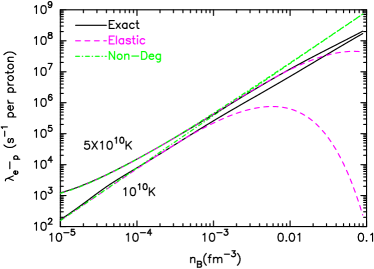
Figure 1: Electron capture rates on protons in SNe matter as a function of the baryon number density $n_{{\hbox{\rm\scriptsize B}}}$ at different temperatures. The electron fraction $Y_{e}$ is taken to be 0.3. The solid curves show the exact results from Eq. (5), the dashed curves are the elastic results from Eq. (13), the dot-dashed curves are the nondegenerate results from Eq. (12).

In the elastic limit, $n_{p}$ in Eq. (12) is replaced by

$$\eta_{pn}=(n_{p}-n_{n})/(1-e^{(\eta_{n}-\eta_{p})/T}).$$ (13)

It is generally believed that electron capture rate under the elastic approximation in some sense introduces the effects of the degeneracy of baryons, so it should be more accurate than that under the nondegenerate approximation. Suppose that the nuclei are dissolved completely into nucleons at high temperature. Figure 1 shows the differences between the exact electron capture rate in the SNe matter and the previous approximate results. The electron fraction $Y_{e}=(n_{e^{-}}-n_{e^{+}})/n_{{\hbox{\rm\scriptsize B}}}$ is assumed to be 0.3, where $n_{{\hbox{\rm\scriptsize B}}}=n_{n}(\mu_{n},T)+n_{p}(\mu_{p},T)$ is the baryon number density. The number density of particles at any degeneracy is expressed in terms of the Fermi-Dirac functions (Aparicio, 1998). The multidimensional integrations and the Fermi-Dirac functions are calculated using the mixture of Gauss-Legendre and Gauss-Laguerre quadratures (Aparicio, 1998). From Fig. 1, it is evident that there are great differences between the elastic results and the exact results when baryons become degenerate. As shown in Eq. (13), the capture rates under the elastic approximation always decrease exponentially when nucleons become degenerate, which is qualitatively correct in the dense nuclear matter near $\beta$-equilibrium. However, this conclusion is not correct obviously in supernova matter. The elastic approximation is also good when $\mu_{p}\simeq\mu_{n}$ because the favored energy transfer is zero. The elastic approximation underestimates the electron capture rate, hopefully, the inclusion of the exact electron capture rate in the future collapsing simulations should be helpful for the supernova explosions.

Condition for kinetic equilibrium.

In principle, if the matter is transparent to neutrinos which carry energy away, the equilibrium of the reactions (1)-(3) can not be treated as a chemical equilibrium problem(Shapiro and Teukolsky, 1983). Suppose that the dynamic time scale of the system under consideration is greater than that of the reactions (1)-(3), the general condition for the kinetic equilibrium is given by

$$\lambda_{e^{-}p}(\mu_{n},\mu_{p},\mu_{e},T)$$

$$=\lambda_{e^{+}n}(\mu_{n},\mu_{p},\mu_{e},T)+\lambda_{n}(\mu_{n},\mu_{p},\mu_{e},T).$$ (14)

However, it is well known that if all the particles involved in the Urca processes are degenerate, such as what happens in the interior of a cold neutron star, then the typical energy of emitted neutrinos is of order the temperature, which could be neglected compared to the Fermi energy of particles, i.e. , $E_{p}+E_{e}=E_{n}$. So the kinetic equilibrium requires $\lambda_{e^{-}p}=\lambda_{n}$ which results in the so-called chemical equilibrium condition for the cold $npe^{-}$ gas,

$$\mu_{n}=\mu_{p}+\mu_{e}.$$ (15)

Before we derive the analytic dynamical equilibrium condition in $e^{\pm}$ plasma with nucleons, we can make some reasonable approximations. First, the rate of neutron decay could be neglected before reaching the degenerate limit. Second, the electrons are nondegenerate, i.e. , $\exp((E_{e}-\mu_{e})/T)\geq 1$. Third, the energy of emitted neutrinos is of order that of the captured electrons/positrons, i.e. , $E_{\nu}\simeq E_{e}$, $E_{\bar{\nu}}\simeq E_{e^{+}}$, and thus $E_{n}\simeq E_{p}$. Under these approximations, $\lambda_{e^{-}p}=\lambda_{e^{+}n}$ gives

$$0 = \lambda_{e^{-}p}-\lambda_{e^{+}n}\propto f_{p}(1-f_{n})f_{e^{+}}$$ (16)

$$\times\left(\frac{e^{(E_{e}+\mu_{e})/T}+1}{e^{(E_{e}-\mu_{e})/T}+1}-e^{((E_{p}-E_{n})-(\mu_{p}-\mu_{n}))/T}\right)$$

$$\simeq f_{p}(1-f_{n})f_{e^{+}}(e^{2\mu_{e}/T}-e^{(\mu_{n}-\mu_{p})/T}).$$

Therefore, from Eq. (16) we obtain the beta-equilibrium condition for the $e^{\pm}$ plasma,

$$\mu_{n}=\mu_{p}+2\mu_{e}.$$ (17)

It should be emphasized that during the above derivation, it is not assumed whether the baryons are degenerate or not. On the other hand, Eq. (17) is still valid under the degeneracy of baryons, which is neglected completely in the approximate reaction rates at the beginning. It is not a surprise to notice that the analytic equilibrium condition Eq. (17) can also be drawn in the completely nondegenerate limit. If all particles are nondegenerate, we have

$$\lambda_{e^{-}p} \propto n_{e^{-}}n_{p}\propto\exp(\eta_{p}+\eta_{e}),$$ (18)

$$\lambda_{e^{+}n} \propto n_{e^{+}}n_{n}\propto\exp(\eta_{n}-\eta_{e}).$$ (19)

From Eq. (18)-(19), the analytic condition Eq. (17) is also obtained heuristically, but not very strictly.

If neutrinos are trapped, the chemical equilibrium condition for both cold $npe^{-}$ and hot $npe^{\pm}$ gases is $\mu_{n}+\mu_{\nu_{e}}=\mu_{p}+\mu_{e}$. The chemical potential of the trapped neutrinos is generally assumed to be zero, thus, Eq. (15) can also be understood as the chemical equilibrium condition for $e^{\pm}$ plasma with neutrino trapping (Beloborodov, 2003a). As $T\rightarrow 0$, the number density of trapped neutrinos $n_{\bar{\nu}_{e}}=n_{\nu_{e}}\propto T^{3}\rightarrow 0$. Therefore, the difference between Eq. (15) and Eq. (17) clearly shows the effects of neutrino trapping.

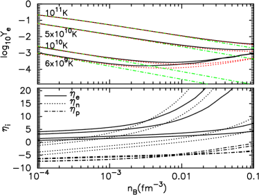
Figure 2: Upper panel: Electron fraction $Y_{e}$ under $\beta$-equilibrium versus the baryon number density $n_{{\hbox{\rm\scriptsize B}}}$ at different temperatures. The solid curves show the exact results from Eqs. (5)-(7), the dotted curves are from the analytic $\beta$-equilibrium condition Eq. (17), and the dot-dashed curves are from the nondegenerate approximation of baryons. Lower panel: The reduced chemical potentials of electrons, neutrons, and protons $\eta_{i}$ as a function of the baryon number density at different temperatures. From top to bottom, the lines correspond to the results of $T=6\times 10^{9}$, $10^{10}$, $5\times 10^{10}$, $10^{11}$K.

Validity of the analytic condition.

The analytic condition Eq. (17) is valid, only if electrons are nondegenerate, which is generally satisfied. If not, the number density of positrons will decrease exponentially. In the following, we check Eq. (17) by numerical calculations. As before, suppose that the nuclei are dissolved completely into nucleons at high temperature. Given the baryon the baryon number density and temperature, the electron fraction $Y_{e}$ is determined by two equilibrium conditions. One is the charge neutrality $n_{e^{-}}(\mu_{e},T)-n_{e^{+}}(\mu_{e},T)=n_{p}(\mu_{p},T)$, the other is the beta equilibrium condition: the integration equation Eq. (14), or our analytic equation Eq. (17). To check the validity of Eq. (17), the equilibrium $Y_{e}$ is calculated based on the exact reaction rates Eqs. (5)-(7), the analytic condition Eq. (17), and the approximate rates, respectively. Figure 2 shows $Y_{e}$ and the reduced chemical potentials $\eta_{i}$ versus the baryon number density at different temperatures. It is evident that the results from the analytic condition are almost consistent with the exact results. The difference occurs only in the regime where electrons become degenerate. As shown in the lower panel of Fig. 2, neutrons become degenerate as electrons do. The particles become degenerate if their reduced chemical potential exceeds the temperature. For electrons and neucleons, their degenerate number densities are estimated to be $n_{e}^{{\hbox{\rm\scriptsize deg}}}\simeq T^{3}/3\pi^{2}\simeq 9.0\times 10^{-6}T_{11}^{3}{\hbox{\rm fm}}^{-3}$, and $n_{n,p}^{{\hbox{\rm\scriptsize deg}}}\simeq(2m_{n,p}T)^{1.5}/3\pi^{2}\simeq 2.8\times 10^{-3}T_{11}^{1.5}{\hbox{\rm fm}}^{-3}$ respectively, where $T_{11}=T/10^{11}$K. In the same regime, there are great differences (of several orders) between our results and the the previous results in which the degeneracy of nucleons is completely neglected. In any case, Fig. 2 evidently shows that the results from the analytic condition are much more accurate than those from the approximate rates in all the parameter regions.

The advantage of having the analytic equilibrium condition at hand is obvious. For instance, we can derive some useful formulae under the nondegenerate approximation. In such limit, $n_{n}/n_{p}=1-1/Y_{e}=\exp((\mu_{n}-\mu_{p}-Q)/T)=\exp((2\mu_{e}-Q)/T)$, Therefore, we have

$$n_{{\hbox{\rm\scriptsize B}}}Y_{e}=\frac{T^{3}}{3\pi^{2}}\left[\left(\frac{\mu_{e}}{T}\right)^{3}+\pi^{2}\left(\frac{\mu_{e}}{T}\right)\right]=\frac{n_{{\hbox{\rm\scriptsize B}}}}{1+e^{(2\mu_{e}-Q)/T}}.$$ (20)

The left equality is exact for the relativistic $e^{\pm}$ (e.g. Blinnikov et al. (1996)). Based on Eq. (20), $\mu_{e}$ and $Y_{e}(\mu_{e})$ can be determined. This simple result completely reproduces the previous numerical results which is corresponding to the dot-dashed curves in Fig. 2. At $\mu_{e}/T<1$ and $(2\mu_{e}-Q)/T<1$, Eq. (20) can be simplified further,

$$Y_{e}=\frac{1}{2}\frac{(1+0.5Q/T)}{(1+1.5n_{{\hbox{\rm\scriptsize B}}}/T^{3})}.$$ (21)

A similar result to Eq. (21) was obtained previously in a different method (Beloborodov, 2003a).

Figure 3: The neutrino emissivity $\epsilon_{\nu}$ versus the baryon number density at different temperatures. The line are the same as those of the upper panel in Fig. 2

The total neutrino emissivity under $\beta$-equilibrium is shown in Fig. 3. Compared with the exact result, both approximate methods overestimate the rate of the neutrino emission because neglecting of the degeneracy of particles increases the phase space for the relevant reactions. It is clearly shown in Fig. 3 that the effect of the neutron degeneracy is much more important than that of electrons, if such conditions are satisfied.