The Spectral Energy Distributions of Infant Super Star Clusters in Henize 2-10 from 7 mm to 6 cm

Abstract

We present observations from our continuing studies of the earliest stages of massive star cluster evolution. In this paper, radio observations from the Very Large Array at 0.7 cm, 1.3 cm, 2 cm, 3.6 cm, and 6 cm are used to map the radio spectral energy distributions and model the physical properties of the ultra-young embedded super star clusters in Henize 2-10. The 0.7 cm flux densities indicate that the young embedded star clusters that are powering the radio detected “ultradense H II regions” (UDH IIs) have masses greater than $\sim 10^{5}M_{\odot}$. We model the radio spectral energy distributions as both constant density H II regions and H II regions with power-law electron density gradients. These models suggest the UDH IIs have radii ranging between $\sim 2-4$ pc and average electron densities of $\sim 10^{3}-10^{4}$ cm^-3 (with peak electron densities reaching values of $\sim 10^{5}-10^{6}$ cm^-3). The pressures implied by these densities are $P/k_{B}\sim 10^{7}-10^{10}$ cm^-3 K, several orders of magnitude higher than typical pressures in the Galactic ISM. The inferred H II masses in the UDH IIs are $\sim 2-8\times 10^{3}M_{\odot}$; these values are $<5$% of the embedded stellar masses, and anonamously low when compared to optically visible young clusters. We suggest that these low H II mass fractions may be a result of the extreme youth of these objects.

1 INTRODUCTION

The study of “super star clusters” (SSCs) has been revolutionized by the availability of high spatial resolution optical observations, such as those obtained with the Hubble Space Telescope (HST). These clusters appear to be common in starburst and merging galaxy systems (Whitmore, 2002), and theory suggests that extreme molecular gas pressures are a prerequisite for their formation (e.g. Elmegreen & Efremov, 1997; Elmegreen, 2002). Many SSCs have properties that are consistent with being adolescent globular clusters (although the necessary conditions for their survival remain unclear, Gallagher & Grebel, 2002).

Compared to globular clusters, SSCs are extremely young objects. However, from a formation perspective, everything has already happened by the time these massive clusters have emerged into optical light (Johnson, 2002). Over the last few years, the study of SSCs has undergone a new revolution with the discovery of ultra-young SSCs that are still deeply embedded in their birth material. The pre-natal clusters have typically been identified in the radio (cm) regime as compact optically thick free-free sources having turnover frequencies $\gtrsim 5$ Ghz. A sample of these objects have now been found in a number of galaxies (e.g. Kobulnicky & Johnson, 1999; Turner, Beck, & Ho, 2000; Tarchi et al., 2000; Neff & Ulvestad, 2000; Johnson et al., 2001; Beck et al., 2002; Plante & Sauvage, 2002; Johnson, Indebetouw, & Pisano, 2003). On a vastly smaller scale, objects with similar spectral morphologies are associated with extremely young massive stars in the Milky Way; these objects are known as “ultracompact H II regions” (UCH IIs) (e.g. Wood & Churchwell, 1989). UCH IIs result from newly formed massive stars that are still embedded in their birth material and ionize compact ($r<<1$ pc) and dense ($n_{e}\gtrsim 10^{4}$ cm^-3) H II regions within their natal cocoons. The apparent similarity between UCH IIs and the scaled-up extragalactic radio sources led Kobulnicky & Johnson (1999) to dub these extragalactic objects “ultradense H II regions” (UDH IIs).

Given the limited observations of UDH IIs that are currently available, attempts to constrain their physical properties have been fairly crude. However, observations have provided estimates for the physical properties of these objects that are truly remarkable: their stellar masses can exceed $\sim 10^{5}M_{\odot}$, the radii of their H II regions are typically a few parsecs, their electron densities suggest pressures of $P/k_{B}\gtrsim 10^{8}$ K, and they appear to have ages of less than $\sim 1$ Myr (Kobulnicky & Johnson, 1999; Vacca, Johnson, & Conti, 2002; Johnson, Indebetouw, & Pisano, 2003). Based on these estimates and comparisons to UCH IIs in the Milky Way, a physical scenario for these ultra-young SSCs has been developed as that of compact (yet massive) clusters of stars that ionize extremely dense H II regions, which are in turn enveloped by warm dust cocoons.

The dense H II regions can be observed in the radio regime, and the radio spectral energy distributions have turnover frequencies that increase with increasing electron density. The dust cocoons can be observed in the infrared to sub-millimeter and may have temperature profiles similar to individual massive protostars in the Milky Way (Vacca, Johnson, & Conti, 2002), although the current lack of observations in these wavelength regimes does not allow rigorous constraints to be placed on the cocoon properties. For example, it is unclear whether the constituent stars are surrounded by individual cocoons, or whether the cocoons have merged and the entire cluster is enveloped in a common cocoon. Presumably the relative morphology of the dust cocoon(s) and the stars depends on both the stellar density and evolutionary state of the cluster. Insufficient radio observations also make it difficult to model the properties of the embedded H II regions; while the nature of a compact radio source (non-thermal, thermal, or optically thick) can be determined from only a pair of high frequency data points, observations at a number of frequencies are required to accurately model spectral turnovers and constrain radii and densities.

In order to distinguish between the different physical regions associated with pre-natal SSCs, throughout this paper we will use the following nomenclature: “cluster” or “SSC” refers only to the embedded stellar content, “UDH II” refers to the dense H II region surrounding the stellar cluster, and “cocoon” refers to the dust cocoon surrounding the H II region.

The starburst galaxy Henize 2-10 (He 2-10) is an excellent system in which to study the properties of ultra-young clusters in detail. At a distance of only 9 Mpc ($H_{0}=75$ km s^-1 Mpc^-1; Vacca & Conti, 1992), it is one of the nearest galaxies known to host multiple UDH IIs (Kobulnicky & Johnson, 1999) as well as a large number of SSCs that have already emerged into optical and ultraviolet light (Johnson et al., 2000; Conti & Vacca, 1994). Mid-IR observations obtained by Vacca, Johnson, & Conti (2002) and Beck, Turner, & Gorjian (2001) confirm that the UDH IIs are surrounded by warm dust cocoons. The dust cocoons surrounding the UDH IIs in He 2-10 are so luminous that Vacca, Johnson, & Conti (2002) find they are responsible for at least 60% of the entire mid-IR flux from this galaxy. This percentage of mid-IR flux due to clusters with ages $\lesssim 1$ Myr old is especially remarkable considering that He 2-10 has been undergoing an intense starburst for several Myr, and hosts nearly 80 optically visible SSCs (Johnson et al., 2000).

The original discovery of the UDH IIs in He 2-10 by Kobulnicky & Johnson (1999) utilized observations at only two radio wavelengths in order to estimate their physical properties. In this paper we present radio observations of the UDH IIs in He 2-10 at five wavelengths (6 cm, 3.6 cm, 2 cm, 1.3 cm, and 0.7 cm) using relatively well-matched synthesized beams in order to more completely map their radio spectral energy distributions and better constrain their physical properties.

2 OBSERVATIONS

We obtained new Q-band (43 Ghz, 0.7 cm), K-band (22 Ghz, 1.3 cm), and U-band (15 Ghz, 2 cm) observations of He 2-10 from February 2001 to January 2003 with the Very Large Array (VLA) . VLA archival data at U-band, X-band (8 Ghz, 3.6 cm), and C-band (5 Ghz, 6 cm) from May 1994 to January 1996 were also retrieved and re-analyzed. All of these data sets are summarized in Table 1. Based on the scatter in the VLA Flux Calibrator database, we estimate the resulting flux density scale at each wavelength is uncertain by $\lesssim 10$%.

Table 1: VLA Observations of He 2-10

$\lambda$	Antenna	Date	Obs. Time	Flux	Phase	Phase Calib.
(cm)	Config.	Observed	(hours)	Calib.	Calib.	$F_{\nu}$ (Jy)
0.7	C-array	2003 Jan 05	3.7	3C286	0836-202	$1.89\pm 0.06$
0.7	C-array	2002 Nov 21	3.8	3C286	0836-202	$2.21\pm 0.04$
1.3	BnA-array	2001 Feb 04	3.1	3C286	0836-202	$2.53\pm 0.05$
2.0	BnA-array	2001 Feb 04	0.5	3C286	0836-202	$2.65\pm 0.09$
2.0	B-array	1996 Jan 03	2.5	3C286	0836-202	$2.98\pm 0.01$
3.6	B-array	1996 Jan 03	0.7	3C286	0836-202	$3.24\pm 0.01$
3.6	A-array	1995 Jun 30	0.5	3C48	0836-202	$2.41\pm 0.06$
3.6	BnA-array	1994 May 14	0.6	3C48	0836-202	$1.90\pm 0.01$
6.0	A-array	1995 Jun 30	1.6	3C48	0836-202	$2.32\pm 0.01$

Calibration was carried out in the Astronomical Image Processing System (AIPS) data reduction package, including gain and phase calibration. The data sets at a given wavelength were combined, and the combined data sets were inverted and cleaned using the task imagr. While the uv-coverages at each wavelength are not identical, an attempt was made to obtain relatively well-matched synthesized beams by varying the weighting used in the imaging process via the “robust” parameter (robust$=5$ invokes purely natural weighting, while a robust$=-5$ invokes purely uniform weighting). The robust values used for each wavelength are listed in Table 2. The synthesized beams at each wavelength obtained with this method are relatively well-matched with the exception of the synthesized beam at 1.3 cm; the synthesized beam at 1.3 cm is approximately 1/3 the area of the beams at the other wavelengths. Therefore, the relative fluxes obtained at 1.3 cm should be regarded as lower limits. In order to facilitate comparison, the final images were all convolved to the same synthesized beam of $0.^{\prime\prime}95\times 0.^{\prime\prime}44$ with a position angle of -3.2 degrees. Figure 1 shows the resulting 0.7 cm contours overlaid on the 3.6 cm grayscale.

Table 2: Imaging Parameters

$\lambda$	Weighting	Synth. Beam	P.A.	RMS noise
(cm)	(robust value)	(${}^{\prime\prime}\times^{\prime\prime}$)	($\arcdeg$)	(mJy/beam)
0.7	1.0	$0.95\times 0.44$	-3	0.07
1.3	5.0	$0.32\times 0.28$	-3	0.05
2.0	1.2	$0.74\times 0.44$	-3	0.05
3.6	0.8	$0.76\times 0.44$	-3	0.03
6.0	2.0	$0.95\times 0.44$	-3	0.05

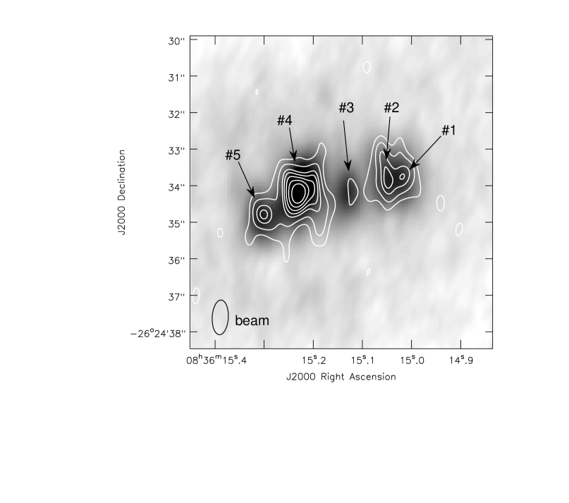
Figure 1: VLA 0.7 cm contours of He 2-10 overlaid on 3.6 cm grayscale. The contour levels are $3,5.0,7,8,9,10,11\times\sigma$ (0.07 mJy/beam).

Flux densities of the sources were measured using two methods. In the first method, the task imfit in AIPS was used to fit the sources with two-dimensional gaussians; the uncertainty from these results was estimated by fitting each source using a range of allowed background estimates and Gaussian profiles. The second method utilized the viewer program in AIPS++ in order to place apertures around the sources at each wavelength; several combinations of apertures and annuli were used in order to estimate the uncertainty in this method. Both of these methods are fairly sensitive to the background level that is adopted, and the uncertainty in the resulting flux densities are dominated by this effect. The resulting flux densities and their uncertainties are listed in Table 3. With the exception of source #4, all of the 2 cm and 6 cm flux densities reported in this paper agree within uncertainty to the values presented by Kobulnicky & Johnson (1999); we attribute the single discrepant case to the different synthesized beams and background estimates used in each analysis.

Table 3: Radio Flux Densities of He 2-10 Sources

	$F_{0.7cm}$	$F_{1.3cm}$	$F_{2cm}$	$F_{3.6cm}$	$F_{6cm}$
Source	(mJy)	(mJy)	(mJy)	(mJy)	(mJy)
1	$0.79\pm 0.13$	$0.66\pm 0.15$	$0.91\pm 0.12$	$0.70\pm 0.14$	$0.61\pm 0.18$
2	$1.08\pm 0.14$	$0.70\pm 0.19$	$0.97\pm 0.14$	$0.87\pm 0.19$	$0.66\pm 0.17$
3	$0.23\pm 0.05$	$0.43\pm 0.15$	$0.68\pm 0.13$	$0.78\pm 0.22$	$0.66\pm 0.18$
4	$2.91\pm 0.57$	$2.36\pm 0.48$	$3.11\pm 0.38$	$3.03\pm 0.52$	$2.26\pm 0.36$
5	$0.89\pm 0.21$	$0.65\pm 0.16$	$0.83\pm 0.15$	$0.76\pm 0.10$	$0.58\pm 0.07$

3 PROPERTIES OF THE UDH IIs

3.1 Production Rate of Ionizing Photons

In order to estimate the embedded stellar content of the UDH IIs in He 2-10, their radio luminosities can be used to determine the production rate of Lyman continuum photons. Following Condon (1992),

$${{Q_{Lyc}}}\geq 6.3\times 10^{52}~{}{{\rm s}^{-1}}\Big{(}{{T_{e}}\over{10^{4}~{}{\rm K}}}\Big{)}^{-0.45}\Big{(}{{\nu}\over{{\rm Ghz}}}\Big{)}^{0.1}\Big{(}{{L_{thermal}}\over{10^{27}~{}{\rm erg~{}s^{-1}~{}Hz}^{-1}}}\Big{)}.$$ (1)

In the application of this equation (which assumes the emission is purely thermal and optically thin), it is advantageous to use measurements made at the highest radio frequency available for two reasons: (1) the higher the frequency, the less likely it is to contain a significant amount of non-thermal contaminating flux, and (2) the higher frequency emission suffers from less self-absorption and is therefore more likely to be optically thin. For these reasons, we use the 43 Ghz (0.7 cm) observations to determine $Q_{Lyc}$ for the UDH IIs in He 2-10. An electron temperature must also be assumed, and we adopt a “typical” H II region temperature of $T_{e}=10^{4}$ K; the uncertainty in $Q_{Lyc}$ due to this assumption is $\lesssim 20$%. The resulting $Q_{Lyc}$ values determined using this method are listed in Table 4, and they range from $Q_{Lyc}\approx 7\times 10^{51}-26\times 10^{51}$ s^-1. To put these values in context, a “typical” O-star (hereafter O*, the equivalent to type O7.5V; Vacca, 1994; Vacca, Garmany, & Shull, 1996) has an ionizing flux of $Q_{Lyc}=1\times 10^{49}$ s^-1. Therefore, the $Q_{Lyc}$ values determined for the UDH IIs in He 2-10 imply the equivalent of 700 - 2600 O*-stars in each cluster.

Table 4: Estimated Properties of the UDH IIs

			Constant Density Models				Density Gradient Models
	$Q_{Lyc}$	Mstars	r	$n_{e}$	MHII			r1/2	$n_{1/2}$	MHII
#	($\times 10^{51}$s-1)	($\times 10^{5}M_{\odot}$)	(pc)	($\times 10^{3}$cm-3)	($\times 10^{3}M_{\odot}$)		$\gamma$	(pc)	($\times 10^{3}$cm-3)	($\times 10^{3}M_{\odot}$)
1	7.1	1.2	$1.8^{+1.1}_{-0.4}$	$6.7^{+3.2}_{-3.7}$	4.0		-0.9	1.7	3.6	5.5
2	9.7	1.6	$1.8^{+0.7}_{-0.4}$	$7.3^{+3.7}_{-3.0}$	4.4		-1.3	2.1	2.4	7.9
4	25.9	4.3	$3.9^{+1.2}_{-0.9}$	$3.9^{+2.1}_{-1.3}$	2.4		-0.0	3.1	3.9	2.4
5	7.9	1.3	$1.7^{+0.4}_{-0.2}$	$7.3^{+1.6}_{-2.1}$	3.7		-1.1	1.9	2.9	6.2

There is an important caveat in regard to the $Q_{Lyc}$ values discussed above. A number of Galactic UCH IIs are observed to be associated with diffuse extended emission. For example, in the Kim & Koo (2001) sample of 16 UCH IIs, all of the objects were associated with extended radio recombination line emission. Likewise, Kurtz et al. (1999) find that 12 out of 15 UCH IIs in their sample are associated with extended emission. These studies conclude that typically $\gtrsim 80$% of the ionizing flux from the embedded stars in UCH IIs is escaping to the outer envelope, possible due to a clumpy density structure within the parent molecular cloud. In the case of He 2-10, there also appears to be a somewhat diffuse thermal background in the immediate vicinity of the UDH IIs. If UDH IIs are leaking ionizing flux in similar proportions to their Galactic counterparts, the inferred stellar content from the $Q_{Lyc}$ values determined above may be a significant underestimate. To estimate an upper limit on the possible leakage of ionizing flux from the UDH IIs, the ionizing flux was measured from the entire region surrounding the UDH IIs. The entire region has an ionizing flux of $Q_{Lyc}\sim 8\times 10^{52}$ s^-1, approximately 40% higher than the sum of the ionizing fluxes from the individual UDH IIs. This “extra” flux is only an upper limit on the ionizing flux that could be escaping from the UDH IIs as it could also be due to contributions from other more evolved clusters in the region.

The masses of the embedded stellar clusters can be estimated from their Lyman continuum fluxes using the Starburst99 models of (Leitherer et al., 1999). For a cluster less than 1 Myr old formed in an instantaneous burst with a Salpeter IMF, 100 $M_{\odot}$ upper cutoff, 1 $M_{\odot}$ lower cutoff (note that reducing the lower mass cutoff to 0.1 $M_{\odot}$ increases the cluster mass by a factor of $\sim 2.5$), and solar metallicity, a $10^{6}M_{\odot}$ cluster has $Q_{Lyc}\approx 6\times 10^{52}$ s^-1. Assuming that $Q_{Lyc}$ scales directly with the cluster mass, we find that the UDH IIs in He 2-10 are powered by stellar clusters with masses $\sim 1.1-4.3\times 10^{5}M_{\odot}$ (Table 4). The mass derived for source 4 from these radio observations is in good agreement with, but a factor of 2 lower than the mass derived by Vacca, Johnson, & Conti (2002) using the bolometric luminosity of the cluster (after taking into account the 0.1 $M_{\odot}$ lower mass cutoff used by Vacca et al.). While the small difference between the mass derived from the radio and bolometric luminosities is certainly contained within the uncertainties, the direction of the difference possibly suggests that a fraction of the ionizing photons are being absorbed by dust within the UDH II. Given the possible leakage of ionizing photons from the UDH IIs and/or their absorption by dust, these mass estimates derived from the radio luminosities are lower limits, and the cluster masses could be as much as $\sim 10\times$ higher than these values.

3.2 Comparison to Model H II Regions

In order to gain additional physical insight about these H II regions, we can invoke simple models. Following the models of Johnson, Indebetouw, & Pisano (2003), we model the compact radio sources as spherical H II regions with constant electron temperature of $10^{4}$ K under two different assumptions: (1) the electron density profile is constant, and (2) the electron density profile is allowed to vary as a power-law of the form $n_{e}\propto r^{\gamma}$. For both sets of models, the flux density measurements at 43 Ghz, 15 Ghz, 8 Ghz, and 5 Ghz were used to fit the models (in a least-squared sense); the 22 Ghz data points were excluded from the models fits as they are only lower limits.

The major difference between these models and those used by Kobulnicky & Johnson (1999) and Johnson et al. (2001) is the allowance for a power-law density profile within a given H II region. We also include limb-darkening, which has an effect in the optically-thin regime at high frequencies. However, the results we obtain with these new models are in excellent agreement with the results from the models used in the above papers; this provides additional confidence in the robustness of the model results. However, the additional radio data points presented in this paper allow us to place more rigorous constraints on the model parameters than Kobulnicky & Johnson (1999).

For the models assuming constant electron density, the data are best fit by H II regions with radii that range between r$\approx 2-4$ pc and electron densities of $n_{e}\approx 4-7\times 10^{3}$ cm^-3. These best fit models are shown with the dashed line in Figure 2. The modeled radii and densities were then used to determine total H II masses of the UDH IIs of $\sim 4-24\times 10^{3}M_{\odot}$. Given that we have two free parameters ($n_{e}$ and r) and four data points, the models are over-constrained and we determine the possible range in the model parameters by finding the minimum and maximum values for $n_{e}$ and r that can fit the data within uncertainty. All of these properties are listed in Table 4.

Figure 2: H II region model fits to the UDH IIs in He 2-10 (source 3 is not included as its spectral energy distribution cannot be fit by a thermal model). The dashed lines are the best fits from the constant density models, and the solid lines are the best fits from the models allowing for a density gradient. Because the synthesized beam at 22 Ghz is significantly smaller than the beams at the other wavelengths, the flux density measured at 22 Ghz is a lower limit and was not used to fit the models.

The second set of models allowed for a density gradient of the form $n_{e}\propto r^{\gamma}$. The main affect of such a gradient on the modeled spectral energy distributions is to make the turnover less abrupt. For sources 1, 2, and 5 these models produce a marginally better fit than the constant density models; the best fit model for source 4 had $\gamma=0$, which is equivalent to the constant density model. These best fit models are shown with a solid line in Figure 2. For these models, the best fit density gradient ($\gamma$), the half-mass radius (r_1/2), the electron density at the half-mass radius ($n_{1/2}$), and the total inferred H II mass (M_HII) are listed in Table 4. For the sources best fit with a density gradient, the electron densities exceed values of $\approx 10^{4}$ cm^-3 in the inner 0.5 pc, and the core densities can reach values close to $\sim 10^{6}$ cm^-3.

The inferred H II mass for each UDH II is $<5$% of the embedded stellar mass ($\sim 3$% -5% for sources 1, 2, and 5, and $\sim 1$% for source 4), which is a strikingly low value when compared to optically visible young clusters. For example, the R136 cluster in the 30 Doradus nebula has a stellar mass of $\sim 6\times 10^{4}M_{\odot}$ (Hunter et al., 1995), but the H II associated with the region has a mass of $\sim 1\times 10^{5}$ (Peck et al., 1997). As the radio observations presented here do not suffer from extinction, it is not likely that the low H II mass fraction for these objects is due to intervening absorption. Instead, we suggest that the low H II mass fraction might be due to the extreme youth of the stellar clusters; much of the gas mass in the vicinity of the cluster may still be shielded from the ionizing radiation, and therefore still in molecular or neutral atomic form.

The densities suggested by the models described above imply tremendously high pressures of $P/k_{B}\sim 10^{7}-10^{10}$ cm^-3 K within the UDH IIs. Pressures of this magnitude are also typical in Galactic UCH IIs (e.g. Churchwell, 1999, and references therein), but they are extremely high compared to typical pressures in the ISM of $P/k_{B}\sim 10^{3}-10^{4}$ cm^-3 K (Jenkins, Jura, & Loewenstein, 1983). These high pressures may be one of the requirements for the formation of SSCs (e.g. Elmegreen & Efremov, 1997; Elmegreen, 2002). However, there are two caveats to bare in mind when considering these estimated pressures: (1) A cluster itself will contribute to the pressure of the surrounding medium. We can estimate the affect of the cluster by assuming the natal H I cloud had a gas temperature of $T_{HI}\sim 10^{2}K$, and the photoionization of the cluster increases the temperature to $T_{HII}\sim 10^{4}K$; therefore, the cluster itself will cause the pressure to increase a factor of $\sim 10^{2}$ over the initial value in the natal cloud. (2) We are not directly measuring the initial pressure of the newborn H II region. Despite the youth of these objects, the H II regions have had some time to expand toward pressure equilibrium. Consequently, the pressures inferred at this stage in their evolution are lower than the initial values. If an H II region expands at a sound speed of roughly $\sim 10$ km/s, it will have expanded from $\sim 1$ pc to $\sim 10$ pc in 1 Myr, causing the pressure to decrease by roughly a factor of $\sim 10^{2}$. These are fairly crude estimates, however even in the case that effect (1) is dominant, the pressures implied for the quiescent natal material are $P/k_{B}\sim 10^{5}-10^{8}$ cm^-3 K.

Source 3 cannot be fit by any purely thermal model (Figure 3). Although this source appears to have a slight turnover around 5 Ghz, the data at the remaining frequencies are fit by a fairly steep negative power-law of $\alpha\sim-1$ (where $S_{\nu}\propto\nu^{\alpha}$), indicating a non-thermal origin. The nature of this source is discussed in Vacca et al. (in prep).

Figure 3: The spectral energy distribution of source 3. This spectral energy distribution cannot be fit by a thermal model.

4 SUMMARY

Multi-frequency radio observations of the deeply embedded massive star forming regions in He 2-10 have allowed us to better constrain their physical properties. The ionizing fluxes calculated from the thermal radio continuum have values ranging from $Q_{Lyc}\approx 7\times 10^{51}-26\times 10^{51}$ s^-1, which imply the clusters have stellar masses $>10^{5}M_{\odot}$. These masses are fully consistent with the masses estimated for the optically visible SSCs by Johnson et al. (2000). We model the H II regions under the assumptions of both constant electron densities and a power-law electron density gradients. These models suggest that the dense H II regions have radii $<4$ pc (and as small as 1.7 pc), and the electron densities may reach values as high as $\sim 10^{6}$ cm^-3 in the cores of these regions. The inferred H II masses for the UDH IIs are $<5$% of the embedded stellar masses, anomalously low compared to optically visible young clusters, and possibly due to the extreme youth of these objects. The densities derived from the models imply pressures of $P/k_{B}\sim 10^{7}-10^{10}$ cm^-3 K within the UDH IIs, typical of Galactic UCH IIs, and provide us with observational confirmation of the extremely high pressures involved in the early stages of super star cluster evolution.

References

- Beck, Turner, & Gorjian (2001) Beck, S.C., Turner, J.L., & Gorjian, V. 2001, AJ, 122, 1365
- Beck et al. (2002) Beck, S.C., Turner, J.L., Langland-Shula, L.E., Meier, D.S., Crosthwaite, L.P., & Gorjian, V. 2002, AJ, 124, 2516
- Churchwell (1999) Churchwell, E. 1999 in: The Origin of Stars and Planetary Systems, C.J. Lada & N.D. Kylafis, Eds. (Kluwer Academic Publishers, 1999), pp. 515-552.
- Condon (1992) Condon, J.J. 1992, ARA&A, 1992, 30, 575
- Conti & Vacca (1994) Conti, P.S. & Vacca, W.D. 1994, ApJL, 423, 97
- Drissen et al. (1995) Drissen, L., Moffat, A.F.J., Walborn, N.R., Shara, M.M. 1995, AJ, 110, 2235
- Elmegreen & Efremov (1997) Elmegreen, B.G. & Efremov, Y.N. 1997, ApJ, 480, 235
- Elmegreen (2002) Elmegreen, B.G. 2002, ApJ, 577, 206
- Gallagher & Grebel (2002) Gallagher, J.S.,III & Grebel, E.K. 2002, IAU Symposium 207, eds. Geisler, Grebel, & Miniti, p. 745
- Hunter et al. (1995) Hunter, D.A.;,Shaya, E.J., Holtzman, J.A., Light, R.M., O’Neil, E.J., Jr., & Lynds, R. 1995, ApJ, 448, 179
- Jenkins, Jura, & Loewenstein (1983) Jenkins, E.B., Jura, M., Loewenstein, M. 1983, ApJ, 270, 88
- Johnson et al. (2000) Johnson, K.E., Leitherer, C., Vacca, W.D., & Conti, P.S. 2000, AJ, 120, 1273
- Johnson et al. (2001) Johnson, K.E., Kobulnicky, H.A., Massey, P., & Conti, P.S. 2001, ApJ, 559, 864
- Johnson (2002) Johnson, K. 2003, Science, 297, 776
- Johnson, Indebetouw, & Pisano (2003) Johnson, K.E., Indebetouw, R., & Pisano 2003, AJ, in press
- Kennicutt (1984) Kennicutt, R.C., Jr. 1984, ApJ, 287, 116
- Kim & Koo (2001) Kim, K-.T. & Koo, B-.C. 2001, ApJ, 549, 979
- Kobulnicky & Johnson (1999) Kobulnicky, H.A. & Johnson, K.E. 1999, ApJ, 527, 154
- Kurtz et al. (1999) Kurtz, S.E., Watson, A.M., Hofner, P., Otte, B. 1999, ApJ, 514, 232
- Leitherer et al. (1999) Leitherer, C., Schaerer, D., Goldader, J.D., Delgado, R.M.G., Robert, C., Kune, D.F., de Mello, D.F., Devost, D., Heckman, T.M. 1999,ApJS, 123, 3
- Moffat, Drissen, & Shara (1994) Moffat, A.F.J., Drissen, L., & Shara, M.M. 1994, ApJ, 436, 183
- Neff & Ulvestad (2000) Neff, S.G. & Ulvestad, J.S. 2000, AJ, 120, 670
- Nürnberger et al. (2002) Nürnberger, D.E.A., Bronfman, L., Yorke, H.W., & Zinnecker, H. 2002, A&A, 394, 253
- Peck et al. (1997) Peck, A.B., Goss, W.M., Dickel, H.R., Roelfsema, P.R., Kesteven, M.J., Dickel, J.R., Milne, D.K., & Points, S.D. 1997, ApJ, 486, 329
- Plante & Sauvage (2002) Plante, S. & Sauvage, M. 2002, AJ, 124, 1995
- Tarchi et al. (2000) Tarchi, A., Neininger, N., Greve, A., Klein, U., Garrington, S.T., Muxlow, T.W.B., Pedlar, A., & Glendenning, B.E. 2000, A&A, 358, 95
- Turner, Beck, & Ho (2000) Turner, J.L., Beck, S.C., & Ho, P.T.P. 2000, ApJ, 532, 109
- Vacca & Conti (1992) Vacca, W.D., & Conti, P.S. 1992, ApJ, 401, 543
- Vacca (1994) Vacca, W.D. 1994, ApJ, 421, 140
- Vacca, Garmany, & Shull (1996) Vacca, W.D., Garmany, C.D., & Shull, J.M. 1996, ApJ, 460, 914
- Vacca, Johnson, & Conti (2002) Vacca, W.D., Johnson, K.E. & Conti, P.S. 2002, AJ, 123, 772
- Whitmore (2002) Whitmore, B.C. 2002, in: A Decade of Hubble Space Telescope Science, M. Livio, K. Noll, M. Stiavelli, Eds. (Cambridge Univ. Press, Cambridge, 2002), pp. 153-180.
- Wood & Churchwell (1989) Wood, D.O., & Churchwell, E. 1989, ApJS, 69, 831