The effects of low temporal frequency modes on minimum variance maps from planck.

We estimate the effects of low temporal frequency modes in the time stream on sky maps such as expected from the planck experiment – a satellite mission designed to image the sky in the microwave band. We perform the computations in a semi-analytic way based on a simple model of planck observations, which permits an insight into the structure of noise correlations of planck-like maps, without doing exact, computationally intensive numerical calculations. We show that, for a set of plausible scanning strategies, marginalization over temporal frequency modes with frequencies lower than the spin frequency of the satellite ($\simeq 1/60$ Hz) causes a nearly negligible deterioration of a quality of the resulting sky maps. We point out that this observation implies that it should be possible to successfully remove effects of long-term time domain parasitic signals from the planck maps during the data analysis stage.

1 Introduction and motivation.

The planck satellite is designed to measure the microwave sky with unprecedented sensitivity and angular resolution. While its primary objective is to characterize the anisotropies in the Cosmic Microwave Background (CMB), the full sky maps in each of the 9 frequency channels will be the true planck legacy.

However, making maps from an instrument like planck is non-trivial, due to the way the sky is scanned and the long-term correlations in the noise properties of the instruments (so-called $1/f$ noise). Though a lot of attention has been given to the long term stability of the planck instrument during its design phase it is practically unavoidable that slow secular drifts and semi-periodic signals will be present in the actual planck data (e.g., Seiffert et al., 2001, Mennella et al., 2002) and will require a software solution. In fact long term drifts, on time scales of hours and longer, are conspicuous in the recent data of the WMAP satellite and have been found to be of sufficient importance that a special treatment was applied to the time ordered data prior to turning them into the sky maps (Hinshaw et al., 2003). It seems therefore prudent to assume that some kind of an analogous procedure will be required to minimize the impact of such effects on the planck maps.

Here we attempt to estimate the magnitude of this impact and elucidate the interplay of those parasitic signals with the usual $1/f$ low frequency tail of the time domain noise as expected for planck. More specifically we investigate two (related) questions. First we strive to gain an understanding of how much the ‘striping’ in a map is constrained by low-frequency information in the time stream (and therefore liable to be compromised by the parasitic signal mentioned above) and how much it is constrained by intersecting scan patterns on the sky. We shall find that the presence of $1/f$ noise at any realistic level means that almost all of our ability to control the low frequency modes comes from the overlap of scan paths in the spatial domain, rather than from long time-scale information in the time stream. Secondly we wish to gain an understanding of how parasitic signals or specific removal techniques affect the structure of the map error matrix. Though for definiteness we will focus hereafter on very specific problems, the analysis presented should be useful in guiding considerations of other similar issues for planck as well as a variety of different experimental setups.

The structure of this paper is as follows. We start with a quick review of map making techniques (Section 2) and present briefly our assumptions about planck, its scanning strategy and anticipated performance (Section 3). In Section 4, we analyze the low temporal frequency problem adopting a time domain perspective, while in Section 5 we derive corresponding pixel domain constraints. These two sections are quite technical, and the reader may wish to skim these on a first pass. We compare both results in Section 6 and finally draw some conclusions in Section 7.

2 Map making review

A reconstruction of a map of the microwave sky from a sequence of measured time ordered data samples is by now a well understood problem (e.g., Wright, Hinshaw, & Bennett, 1996, Tegmark, 1997a, Stompor et al., 2002). An entire suite of approaches, ranging from a simple binning of observations into pixels on the sky, through destriping techniques to optimal minimum variance map-making, has been to date successfully implemented, investigated in detail (e.g., Wright et al., 1996, Tegmark, 1997b, Delabrouille, 1998, Borrill et al., 2000, Natoli et al., 2001, Doré et al., 2001, Maino et al., 2002) and in a handful of cases converted into publicly available software packages (e.g., MADCAP, MAPCUMBA, MADmap). These different approaches trade, to various degrees, simplicity and numerical speed for accuracy of the produced maps, and usually they can be derived either as a special case of, or an approximation to, a more general formalism based on a maximum likelihood approach to map-making. The latter provides a handy and concise algebraic formulation of the entire problem (Tegmark, 1996). It has been demonstrated within such a formalism that a number of relatively straightforward generalizations are possible allowing us, in a statistically strict manner, to account for a variety of systematic problems commonly troubling actual experimental data (Wright et al., 1996, Oliveira-daCosta et al., 1999, Stompor et al., 2002, Hinshaw et al., 2003). All these developments highlight the practical feasibility, flexibility and robustness of this approach. In this context a major task in a successful accomplishment of the map-making stage for any CMB experiment becomes the detection and characterization of systematic contributions plaguing real data sets. The problem is made more difficult by the sheer size and complexity of current and future data sets. Consequently, for map-making practitioners, the map-making issue is far from being definitely resolved and keeps providing challenges on a case-by-case basis.

In a standard map-making procedure (Tegmark 1997a, Borrill et al., 2000) a final uncertainty of the map is encoded in a pixel-pixel noise correlation matrix. In the case of a Gaussian instrumental noise, this matrix provides a complete description of the map error. However, in most of circumstances of the interest, given the size of forthcoming maps, the computation and storing of such a matrix is prohibitive, let alone any investigation of its structure and its dependence on a presence of parasitic signals in the data, or on details of a removal technique applied to such a systematic. In such cases an understanding of a role of a particular systematic effect and its impact on the final map needs to be investigated by different usually more indirect and simplified means.

3 planck – basic features.

To elucidate the impact of instrumental parasitics on low temporal frequencies (generally understood hereafter as those lower than the satellite spin frequency) we construct a simple model of planck which captures all of the essential features for our purposes. We assume that the satellite spins on its axis roughly once per minute (${t_{\mathrm{spin}}}\equiv{1/{f_{\mathrm{spin}}}}=1$min), with any given detector beam sweeping out a circle (or more generally – following Wandelt & Górski, 2001, and Wandelt & Hansen, 2003 – a basic scan path) on the sky with opening angle of $2\theta_{0}=170^{\circ}$. We will refer to a short stretch of a circle (ring) of a beam-size length as a ring pixel. The sampling rate is assumed to be ${\Delta_{\mathrm{s}}}=(\theta_{\mathrm{fwhm}}/3)/(11800{f_{\mathrm{spin}}})$, corresponding to three measurements per the FWHM of a detector beam ($\equiv\theta_{\mathrm{fwhm}}$) at each passing. Hereafter, whenever needed we will assume that $\theta_{\mathrm{fwhm}}=10^{\prime}$. Each circle is observed for $1$hour, before the satellite axis re-points and a different ring (shifted with respect to the previous one by $\sim 2.5^{\prime}$ along the great circle on the sky) is observed for another time $T$. We will assume that the re-pointing from a circle to a next one is always instantaneous. As the satellite axis is re-pointed only by $\sim 2.5^{\prime}$ every hour, during every four hour long period each detector of the satellite observes approximately the same sky sweeping during that time a single ring of a beam-size width. Hence, hereafter as basic scan paths we will consider sky rings as swept out during a time period of $T=4$hours. The re-pointing frequency is thus, ${f_{\mathrm{rpt}}}=1/T\simeq 7\cdot 10^{-5}$Hz. The number of scans of each ring is ${T/{t_{\mathrm{spin}}}}$ and there are ${n_{\mathrm{rpix}}}$ (beam size) ring pixels per ring. As we will discuss in some detail in Sect. 5.1, ${n_{\mathrm{rpix}}}$ also corresponds to a number of (nearly) uncorrelated, independent ring pixels for a single ring of a planck-like experiment and is therefore an important factor in the scaling relations of the pixel domain noise properties derived in the following.

We should emphasize that though the discussion presented here touches upon and depends upon a number of scan-related assumptions, the issues involved in optimizing the scanning strategy for planck are more complex and varied than what is included in the discussion presented below. Clearly a more pointed analysis is required to elaborate on those issues. We leave such a discussion for future work. As far as this paper is concerned, while it is clear the numerical prefactors in our results are dependent on a particular scanning strategy, we believe that our main conclusions are independent on their specific details.

Hereafter, we assume that the Gaussian instrumental noise can be accurately described as,

$$P\left({f_{\mathrm{t}}}\right)={\sigma_{\mathrm{t}}}^{2}\,{\Delta_{\mathrm{s}}}\,\left(1+{{f_{\mathrm{knee}}}\over{f_{\mathrm{t}}}}\right),$$ (1)

where ${f_{\mathrm{t}}}$ is a temporal frequency, ${f_{\mathrm{knee}}}$ and ${\sigma_{\mathrm{t}}}^{2}$ parameterize the spectrum, and, ${\sigma_{\mathrm{t}}}$ describes the (white) noise level per measurement. Both these values are strongly detector-dependent. In the following, whenever necessary, we will assume the following values: for hfi, ${f_{\mathrm{knee}}}\simeq 30$mHz and ${\sigma_{\mathrm{t}}}\simeq 1000\mu\mathrm{K}\ (\simeq 100\mu\mathrm{K}\sqrt{\mathrm{sec}}/\sqrt{{\Delta_{\mathrm{s}}}})$ and for lfi, ${f_{\mathrm{knee}}}\simeq 50$mHz and ${\sigma_{\mathrm{t}}}\simeq 3000\mu\mathrm{K}\ (\simeq 300\mu\mathrm{K}\sqrt{\mathrm{sec}}/\sqrt{{\Delta_{\mathrm{s}}}})$ (in both cases in antenna units). Here, hfi and lfi refer to the High and Low Frequency Instruments of planck respectively. The actual flight parameters may be somewhat better. However, for any anticipated values of ${f_{\mathrm{knee}}}$ the following relation is satisfied,

$${f_{\mathrm{rpt}}}\ll{f_{\mathrm{spin}}}\lower 2.15277pt\hbox{$\;\buildrel<\over{\sim}\;$}{f_{\mathrm{knee}}}.$$ (2)

As it is discussed below, our conclusions will not be affected by changes of either the noise level, which will only lead to a rescaling of the estimated values, or the assumed values of ${f_{\mathrm{knee}}}$ as long as these are larger than $\lower 2.15277pt\hbox{$\;\buildrel>\over{\sim}\;$}1$mHz.

4 Time domain considerations.

4.1 Background

The generalized least squares map-making starts by modeling the observation as

$$t=As+n$$ (3)

where $t$ indicates the time stream data, $A$ is the pointing matrix, $s$ the sky signal and $n$ the noise. If ${\cal N}_{\mathrm{t}}=\langle nn^{t}\rangle$ is the (time-domain) noise correlation matrix, the minimum variance estimator of the sky signal, $m$, is

$$m=\left[A^{t}{\cal N}_{\mathrm{t}}^{-1}A\right]^{-1}A^{t}{\cal N}_{\mathrm{t}}^{-1}t$$ (4)

with $\left[A^{t}{\cal N}_{\mathrm{t}}^{-1}A\right]^{-1}$ the pixel-pixel noise correlation matrix. This equation can be efficiently solved using iterative methods if ${\cal N}_{\mathrm{t}}$ is known (Doré et al., 2001, Natoli et al., 2001). Those methods do not require explicit computations of the pixel-pixel noise correlation matrix – a property which makes solving for the map estimate feasible from both CPU time and disk/memory storage points of view.

Clearly, in this equation two kinds of constraints are incorporated: first based on the known correlations in the time domain, as given by the noise correlation matrix, ${\cal N}_{\mathrm{t}}$, and second based on the fact that some parts of the (unchangeable by definition) sky are observed multiple times during an experiment, as encoded in the pointing matrix, $A$. Both constraints are usually tightly combined together, e.g., as seen in Eq. 4, giving us the ‘best’ possible map estimate, for instance, that with a minimum noise variance.

Efforts to remove/minimize systematic effects present on the time stream level can affect both of these types of constraints to a different extent. If, for instance, entire stretches of the time ordered data stream are rendered unusable and effectively removed from the data, some pixels on the sky may not be observed multiple times anymore or even observed at all, clearly affecting the strength of the pixel domain constraints. If, in the contrary, only some of the temporal frequency bands have been found to be compromised by a systematic effect, it will be time domain constraints which will be affected more directly.

In the following we will focus on the latter case assuming that only low temporal frequencies have been contaminated by a systematic effect of some kind but no time samples have had to be removed and therefore no changes to an actual scan pattern observed on the sky have been made.

4.2 Destriping vs optimal map-making for planck.

Given the rather simple scanning strategies planned for planck, the sky map recovery can proceed in a number of ways. In particular, multiple re-scanning of the successive rings on the sky opens up the possibility of performing map-making in two stages. In this case, first maps of the single rings are created which are subsequently combined together using the fact that different rings cross each other multiple times on the sky, i.e., exploiting the pixel domain constraint in a parlance of the previous Section. Such a two-step approach is a keystone of the destriping methods (Dellabrouile, 1998, Maino et al., 2002, Keihanen et al., 2003). Techniques of this kind are in general not optimal. That is the case even if single ring maps are produced using optimal map-making (as we will assume in this paper henceforth), rather than simple sky binning as in ‘traditional’ destriping. This fact can be understood as follows. As long as the beam is simply sweeping the sky in a circle, in the frequency domain the sky signal is concentrated only at harmonics of the spin period and at zero frequency. The latter contains not only actual sky monopole but also all the higher multipole moments which do not average to zero over the circle. All together, these contributions amount to a constant ring offset. In a total power CMB experiment the constant offset of a single segment of the time ordered data is usually lost, leading to a loss of the ring offsets together with the corresponding part of the actual sky signal.

Let us assume now that after spending time $T$ on a given ring, the observation continues and the instrument is re-pointed and a scan of another circle commences, as it is the case for planck. In the destriping methods, the continuity of the time stream from a ring to ring is ignored, and each ring is analyzed separately. Consequently, as in a single ring case mentioned above, the offsets of all the rings are lost during the initial single-ring processing and need to be subsequently restored (from now on only relative). The uncertainty involved in such a procedure increases the effective noise level in the map and a noisier map results. The situation looks different in the methods in which the time stream is not cut into segments, which are then analyzed separately, but treat the time stream in its entirety. Indeed, if the re-pointing is performed without interrupting the time stream continuity, the sky signal formerly confined to the zero frequency mode and the spin frequency harmonics, now partially resides at the harmonics of the re-pointing frequency ${f_{\mathrm{rpt}}}(=1/T)$ and at sidebands of the harmonics of the spin frequency (i.e., $f={f_{\mathrm{spin}}}\pm{f_{\mathrm{rpt}}},{f_{\mathrm{spin}}}\pm 2{f_{\mathrm{rpt}}},\dots;2{f_{\mathrm{spin}}}\pm{f_{\mathrm{rpt}}},2{f_{\mathrm{spin}}}\pm 2{f_{\mathrm{rpt}}},\dots,$ etc) as well. Though the zero frequency mode is again lost, all the signal confined to the non-zero frequency bands is in principle accessible, rendering tighter constraints on the recovered sky map. If the instrument is successively and smoothly re-pointed in such a way that the observed sky area progressively increases, more of the multipole moments of the map are contained in non-zero frequencies. In the case of a full sky covered in such a way, only the sky monopole would be lost together with the zero frequency mode.

In the following we address the issue of how much of an actual improvement over the two step method can be expected from such an approach in a case of a realistic planck-like experiment. Given that, on the ring level, the two-stage method exploits only the pixel domain constraints, while the full optimal map-making attempts to make use of both pixel and time domain ones, this question is clearly just a rephrasing of the problem posed in the previous Section. At the computational level we can turn this problem into a question of how the time domain derived constraints on the relative offsets of two rings compare with those derived from the pixel domain. Alternately, as uncertainty in the recovery of the rings offsets results in the presence of strongly correlated linear features in the map aligned with the scan direction (i.e., stripes), we will refer to that problem as striping.

The attractive advantage of the two-step map-making is its robustness to low frequency parasitic signal removal. Indeed, if the parasitic signal is confined to the frequency range $f\leq{f_{\mathrm{marg}}}\lower 2.15277pt\hbox{$\;\buildrel<\over{\sim}\;$}{f_{\mathrm{spin}}}$, then high-pass filtering that part of the time stream which comes from each ring can remove most non-cosmological signals and at most an offset in the sky signal, causing no extra loss in precision. By contrast, the loss of the precision of the optimal map-making incurred due to a removal of the contaminated low frequency modes needs to be investigated in detail (see Section 4.3).

At this point it is worth emphasizing two issues. First, in the case of planck, where ${f_{\mathrm{knee}}}>{f_{\mathrm{spin}}}$, if the final solution is to be nearly optimal it may need to account for the presence of $1/f$ noise within each ring. This suggests that Eq. 4 be solved on each ring (see Sect. 5.1) as the first step of the destriping method. Second, in this paper we will use the words filtering and marginalization over a given frequency band interchangeably, always meaning the latter. Henceforth, marginalization (or filtering) is understood as a procedure of “weighting-out” unwanted frequency modes from the final map and the corresponding map noise correlation matrix by setting the noise level in those modes to infinity (i.e., the weights to zero). In both cases the relevant operations are usually done in Fourier space. More details on this approach can be found in the next Section and elsewhere (e.g., Stompor et al., 2002).

Of course, the marginalization over the frequency band is not the only way of dealing with the parasitic signal. Other options can be viable, especially if extra information about the origin or character of the problem is available (e.g., Stompor et al. 2002). By comparison the marginalization may look like quite a drastic approach. However, as we show that in the following, for the low temporal frequency parasitic signal the marginalization turns out to be as good an approach as any other and more generally applicable.

4.3 Constraining offsets.

The questions of interest then are how important the low-frequency information contained in ${\cal N}_{\mathrm{t}}$ is in reducing the the stripiness in the maps and how it depends on filtering out progressively higher frequencies. These questions can be rephrased as the following: suppose we observe two rings during time $2T$. If there is no sky signal, how well can we constrain a relative offset, $\delta$, between the two rings using the data $t$? The variance in the offset obtained by generalized least squares is $\left[A^{t}{\cal N}_{\mathrm{t}}^{-1}A\right]^{-1}$ where now $A=[0,0,\cdots,0,0,1,1,\cdots,1,1]^{t}$ describes the effects of the offset on the time stream. If the noise is stationary with power spectrum as in Eq. 1 then the (inverse) variance is

$$\sigma_{\delta}^{-2}={1\over 4}\sum_{k}\ {\left|{W_{\mathrm{0}}}\left({f_{\mathrm{k}}}T\right)\right|^{2}\over P({f_{\mathrm{k}}})},$$ (5)

where the sum is over frequencies ${f_{\mathrm{k}}}=k/2T$ from 0 up to the Nyquist frequency and ${W_{\mathrm{0}}}/2$ is the Fourier transform of the pointing matrix $A$ which is given, up to a phase, by

$${W_{\mathrm{0}}}\left(x\right)\equiv j_{0}\left(\pi x\right)$$ (6)

where ${j_{\mathrm{0}}}(x)\equiv\sin(x)/x$ is the spherical Bessel function of order zero. If the marginalization is performed the amplitude of the inverse noise power spectrum is set to zero for all frequencies $f\leq{f_{\mathrm{marg}}}$ and $\sigma_{\delta}$ correspondingly increases.

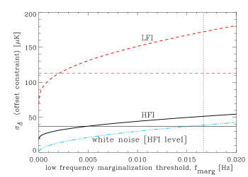
Figure 1: The dependence of the time domain constraint on relative offsets as a function of the low frequency marginalization threshold (${f_{\mathrm{marg}}}$). Three curved lines correspond to the fiducial LFI, HFI and HFI-like white noise cases, respectively from top to bottom. For comparison, the nearly horizontal lines show the noise per beam-size pixel for LFI (top line) and HFI (bottom). The dotted vertical line shows the spin frequency of the planck satellite.

The rate of that increase depends on the assumed noise power spectrum parameters as shown in Fig. 1. It is clear that the mere presence of the $1/f$ component in the spectrum is nearly as harmful as the marginalization itself. That is because in such a case the noise power at frequencies $f\ll{f_{\mathrm{knee}}}$ is sufficiently high to effectively “weight out” (i.e., to marginalize over) the lowest frequency tail. Therefore in the absence of the $1/f$ noise the losses suffered due to the low-frequency marginalization are the largest. By the same token the time domain constraints are the strongest in a white noise case, though the dependence of $\sigma_{\delta}$ on ${f_{\mathrm{knee}}}$ disappears once ${f_{\mathrm{marg}}}\gg{f_{\mathrm{knee}}}$. For values of ${f_{\mathrm{marg}}}$ of interest here (i.e., ${f_{\mathrm{marg}}}\lower 2.15277pt\hbox{$\;\buildrel<\over{\sim}\;$}{f_{\mathrm{spin}}}\ll 1/2{\Delta_{\mathrm{s}}}$) and any ${f_{\mathrm{knee}}}(\geq 0)$ the following approximate formula holds to within few percent,

$$\sigma_{\delta}^{2}\simeq{\sigma_{\mathrm{t}}}^{2}{\pi^{2}{f_{\mathrm{knee}}}\;{\Delta_{\mathrm{s}}}\over\log\left(\displaystyle{{f_{\mathrm{knee}}}+{f_{\mathrm{marg}}}+{f_{\mathrm{1}}}}\right)-\log\left(\displaystyle{{f_{\mathrm{marg}}}+{f_{\mathrm{1}}}}\right)},$$ (7)

here, ${f_{\mathrm{1}}}=1/2T\simeq 3.5\cdot 10^{-5}$Hz. This formula together with Fig. 1 are the main results of this Section.

Note that in a more realistic case the available time stream data set will be composed of many ring segments of length $T$. Therefore, rather than the single parameter case as in Eq. 5 we should consider a case with multiple offsets each assigned to a different stretch of the time stream and derive the constraints also for the relative offsets of the non-adjacent segments. Instead of deriving the appropriate formulas (which are a straightforward generalization of the single offset case considered above and follow the same basic steps as presented in the next Section), we just note that the relative offset of two segments becomes progressively less constrained if the time separation of these two segments increases. That is a consequence of the extra noise power present at the low frequency end of the spectrum either due to a generic, $1/f$, noise component or the low frequency marginalization. Therefore if there is any gain as a result of incorporating the time domain constraints on the relative offsets it should be the most significant on the shortest time scales. Hence we conclude that the formulas derived above, Eq. 5 & Eq. 7, indeed provide the best case answer to be confronted with the pixel domain constraints derived later on.

5 Pixel (ring) domain considerations

5.1 Ring-noise properties.

Let $A$ be now a pointing matrix from the time domain to a ring pixel domain. Then, as usual, noise correlations in the ring domain can be expressed as,

$${\cal N}_{\mathrm{r}}=\left(A^{t}{\cal N}_{\mathrm{t}}^{-1}A\right)^{-1}.$$ (8)

With crossing time of a single beam-size pixel denoted as ${t_{\mathrm{rpix}}}$ ($={{t_{\mathrm{spin}}}/{n_{\mathrm{rpix}}}}$), the pointing matrix, for a single ring, is given by:

$$A\left(t,\ k\right)=1;\ \ \ t-t\;\rm{mod}\;{t_{\mathrm{rpix}}}=k\;{t_{\mathrm{spin}}},$$ (9)

and is zero otherwise. Here we number the pixels in a way that ring pixel $0$ is observed at $t=0$. Given a consecutive and linear pixel numbering along a ring circumference we have,

$$A\left(t,\ k^{\prime}\right)=A\left(t+\left(k^{\prime}-k\right)\;{t_{\mathrm{rpix}}},\ k\right),$$ (10)

for any two pixels $k$ and $k^{\prime}$.

Rewriting Eq.(8) in a Fourier domain (and assuming circulancy of ${\cal N}_{\mathrm{t}}$) we have,

$${\cal N}_{\mathrm{r}}=\left[\left(FA\right)^{T}\mathrm{diag}\left[{P\left(f_{t}\right)^{-1}}\right]\left(FA)\right)\right]^{-1}.$$ (11)

here $F$ is a Fourier operator. From Eq.(10)

$$\left(FA\right)_{\mathrm{k}}=\exp{\left(-\iota\,2\pi{f_{\mathrm{t}}}k\;{t_{\mathrm{rpix}}}\right)}\left(FA\right)_{\mathrm{k=0}}.$$ (12)

From Eq.(9)

$$\left(FA\right)_{\mathrm{k=0}}={W_{\mathrm{0}}}\left({f_{\mathrm{t}}}\;{t_{\mathrm{rpix}}}\right){W_{\mathrm{1}}}\left({f_{\mathrm{t}}}\;{t_{\mathrm{spin}}},\;T/{t_{\mathrm{spin}}}\right)$$ (13)

where

$${W_{\mathrm{1}}}\left(x,\;n\right) \equiv {\sin{\displaystyle{(n+1)\pi x}}\over\sin{\displaystyle{\pi x}}}\exp{\left(-\iota\,\displaystyle{n\pi x}\right)},$$ (14)

and ${W_{\mathrm{0}}}$ was defined in Eq. 6. Let us assume translational symmetry along the ring, neglecting therefore “switching on and off” effects, the noise correlation in pixel domain can be expressed via “ring domain” power spectrum, ${\cal P}\left({f_{\mathrm{r}}}\right)$, where ${f_{\mathrm{r}}}$ is a ring domain frequency expressed in Herz. The inverse noise spectrum in the ring domain is then given as,

$${\cal P}\left({f_{\mathrm{r}}}\right)^{-1} = \sum_{\Delta k,\;{f_{\mathrm{t}}}}\left|{W_{\mathrm{1}}}\left({f_{\mathrm{t}}}\;{t_{\mathrm{spin}}},\;T/{t_{\mathrm{spin}}}\right)\right|^{2}\left|{W_{\mathrm{0}}}\left({f_{\mathrm{t}}}\;{t_{\mathrm{rpix}}}\right)\right|^{2}$$ (15)

$$\times P\left({f_{\mathrm{t}}}\right)^{-1}\exp{\left(-\iota 2\pi\left({f_{\mathrm{t}}}-{f_{\mathrm{r}}}\right)\Delta k\;{t_{\mathrm{rpix}}}\right)}$$

$$= \sum_{{f_{\mathrm{t}}}}\;\left|{W_{\mathrm{1}}}\left({f_{\mathrm{t}}}\;{t_{\mathrm{spin}}},\;T/{t_{\mathrm{spin}}}\right)\right|^{2}\left|{W_{\mathrm{0}}}\left({f_{\mathrm{t}}}\;{t_{\mathrm{rpix}}}\right)\right|^{2}$$

$$\times {W_{\mathrm{1}}}^{\Re}\left(\pi\left({f_{\mathrm{t}}}-{f_{\mathrm{r}}}\right){t_{\mathrm{rpix}}},{n_{\mathrm{rpix}}}\right)\;P\left({f_{\mathrm{t}}}\right)^{-1}.$$

Here, the superscript $\Re$ denotes a real part. The noise correlation matrix can be computed via a Fourier transform,

$${\cal N}_{\mathrm{r}}=F^{T}\;\mathrm{diag}\left[{\cal P}\left({f_{\mathrm{r}}}\right)\right]\;F.$$ (16)

Though this result looks very intuitive, the expression for ${\cal P}\left({f_{\mathrm{r}}}\right)$ is less so. Nevertheless, for the set of parameter values as described in Sect. 3, the resulting ring-domain power spectrum turns out to be basically a time-domain spectrum resampled on a sparser grid of frequencies corresponding to the ring domain. The corresponding ring domain ${f_{\mathrm{knee}}}$ is nearly identical to that in the time domain, and the resampling ensures that the marginalization over all frequencies $f\leq{f_{\mathrm{marg}}}$ does not cause any singularities of the ring domain noise correlation matrix in addition to that at zero frequency as long as ${f_{\mathrm{marg}}}<{f_{\mathrm{spin}}}$, i.e., in that case ${\cal P}\left({f_{\mathrm{r}}}\right)^{-1}>0$, if ${f_{\mathrm{r}}}\neq 0$, and ${\cal P}\left({f_{\mathrm{r}}}\right)$ is well-defined. For the beam-size pixels, we find that the off-diagonal noise correlations in the ring domain are usually less than a percent of the rms noise value per ring pixel, given by,

$${\sigma_{\mathrm{r}}}^{2}={1\over{t_{\mathrm{rpix}}}}\sum_{{f_{\mathrm{r}}}}{\cal P}\left({f_{\mathrm{r}}}\right).$$ (17)

In the following, we will therefore neglect these off-diagonal correlations and consistently keep assuming that the number of independent, uncorrelated ring elements is equal to the number of beam size ring pixels, ${n_{\mathrm{rpix}}}$. It is important to point out that the assumption made above does not automatically force the noise correlations of a final map to be also diagonal. We discuss that issue further below.

Having estimated the noise correlation matrix, ${\cal N}_{\mathrm{r}}$, we can also estimate the ring map using Eq. 4. In the following, in the spirit of the destriping methods we will reconstruct the sky maps via combining all the precomputed sky rings paying a particular attention to the noise correlation patterns of the resulting sky maps and the precision of the recovery of the relative ring offsets.

5.2 Offsets from ring crossings.

In this Section we will proceed assuming that there are no off-diagonal noise correlations within each ring. This assumption has been justified above. We will show below that this assumption does not mean that there will be no correlations in the final map, made as a superposition of all the rings on the sky. We will estimate these correlations as well as dispersions and compare the results with the time domain constraints derived earlier.

Yet again, let us define a simple map-making problem, this time the projection is performed from sky pixel domain, as for example defined by healpix (Górski et al. 1998), to the ring domain. From a set of all ring pixels for all the sky rings we choose only ring-pixels which cross with at least one other ring. We form a vector, $r$, of all estimated temperature values for all such ring pixels. These are derived from the time ordered data as described in the previous Section. We assume that each of the ring pixels included above corresponds to a certain uniquely defined sky pixel. Though this may not always be the case, as some ring pixels may span more than a single sky pixel, it is a useful simplification which we expect to be broken only occasionally. We number the sky pixels consecutively counting each pixel once and form a vector of the corresponding true sky temperatures denoted, $s$. Consequently, any ring pixel temperature, $r_{\mathrm{i}}$, can be modeled as a sky temperature in a corresponding sky pixel, $s_{\mathrm{j}}$, plus a ring-pixel instrument noise, $n_{\mathrm{i}}$ and its own specific offset, $x_{\mathrm{k}}$. The latter contributes to any measurement made along a given ring. Hence we get,

$$r=As+n+Bx=[A,B]\left[\begin{array}[]{c}\displaystyle{s}\\ \displaystyle{x}\end{array}\right]+n.$$ (18)

In the above equation, $A$ is a pointing matrix assigning which sky pixel was observed at which measurement, and a matrix, $B$, is deciding to which ring a given ring-pixel belonged and therefore which offset $x$ is to be added to it. Under our assumptions, the noise correlation matrix, ${\cal N}_{\mathrm{r}}=\langle nn^{t}\rangle$, is diagonal and all of its diagonal elements are identical and denoted as, ${\sigma_{\mathrm{r}}}^{2}$.

Our task here is to solve this system of equations to estimate the noise properties of the recovered “map”, $m$, which includes estimates of both the actual sky, $s$, and ring offsets, $x$. The resulting noise correlation matrix is as usual given as,

$${\cal N}_{\mathrm{s}}=\left([A,B]^{t}{\cal N}_{\mathrm{r}}^{-1}[A,B]\right)^{-1}={\sigma_{\mathrm{r}}}^{2}\left[\begin{array}[]{c c c}\displaystyle{A^{t}A}&&\displaystyle{A^{t}B}\\ \displaystyle{B^{t}A}&&\displaystyle{B^{t}B}\end{array}\right]^{-1}.$$ (19)

Hereafter we will denote the matrix on the right hand side of this equation with, ${\cal A}$. This matrix has a block structure with two diagonal blocks describing the correlations between the sky pixels and the offsets respectively, the two off-diagonal blocks characterize the cross-correlations between them. Of course, not all ring pixels are involved in this map-making problem explicitly, but only those which are observed during at least two different ring scans. The correlations between remaining pixels are equal to the correlations between offsets of the rings they happen to be intersected by. For well-cross-linked scanning strategies, where most of the pixels are observed multiple times, from various directions, the pixel-pixel correlations need to be computed directly or based on considerations such as those presented here. In either case the level of stripiness in the maps can be measured as an RMS difference between the amplitudes of two rings given by,

$$\sigma_{\delta}=\sqrt{2\left({\sigma_{\mathrm{off}}}^{2}-{X_{\mathrm{off}}}\right)},$$ (20)

where ${\sigma_{\mathrm{off}}}$ and ${X_{\mathrm{off}}}$ are the variance of the ring offsets recovery and a cross-correlation between two offsets.

In general calculating ${\cal N}_{\mathrm{s}}$ in Eq. 19 is difficult and commonly requires extensive numerical computations, which easily become prohibitively expensive. Instead of doing that here we will consider a set of toy models to gain insight into the structure of the resulting noise correlations.

5.2.1 two rings

Let us begin with a pair of two intersecting rings (or more generally, basic scan paths). Let the number of crossings (i.e., pixels in common between the rings) be, ${n_{\mathrm{cross}}}$. To break a degeneracy due to the unknown and unrecoverable absolute offset of these rings, we constrain the offset of the 1st ring to be 0. Recalling that every crossed pixel is observed twice, the matrix in Eq. 19 in this case reads,

$${\cal A}=\left[\begin{array}[]{c c}\displaystyle{A^{t}A,}&\displaystyle{A^{t}B}\\ \displaystyle{B^{t}A,}&\displaystyle{B^{t}B}\end{array}\right]=\left[\begin{array}[]{c c c c c}\displaystyle{2}&\displaystyle{0}&\displaystyle{\cdots}&\displaystyle{0}&\displaystyle{1}\\ \displaystyle{0}&\displaystyle{2}&\displaystyle{\cdots}&\displaystyle{0}&\displaystyle{1}\\ \displaystyle{\vdots}&\displaystyle{\vdots}&\displaystyle{\ddots}&\displaystyle{\vdots}&\displaystyle{\vdots}\\ \displaystyle{0}&\displaystyle{0}&\displaystyle{\cdots}&\displaystyle{2}&\displaystyle{1}\\ \displaystyle{1}&\displaystyle{1}&\displaystyle{\cdots}&\displaystyle{1}&\displaystyle{{n_{\mathrm{cross}}}}\\ \end{array}\right],$$ (21)

where the last column and row correspond to the offset of the second ring. The inverse of ${\cal A}$ is readily given by,

$${\cal A}^{-1} = \left[\begin{array}[]{c c}\displaystyle{A^{t}A,}&\displaystyle{A^{t}B}\\ \displaystyle{B^{t}A,}&\displaystyle{B^{t}B}\end{array}\right]^{-1}={1\over 2{n_{\mathrm{cross}}}}\times$$ (24)

$$\times \left[\begin{array}[]{c c c c c}\displaystyle{{n_{\mathrm{cross}}}+1}&\displaystyle{1}&\displaystyle{\cdots}&\displaystyle{1}&\displaystyle{-2}\\ \displaystyle{1}&\displaystyle{{n_{\mathrm{cross}}}+1}&\displaystyle{\cdots}&\displaystyle{1}&\displaystyle{-2}\\ \displaystyle{\vdots}&\displaystyle{\vdots}&\displaystyle{\ddots}&\displaystyle{\vdots}&\displaystyle{\vdots}\\ \displaystyle{1}&\displaystyle{1}&\displaystyle{\cdots}&\displaystyle{{n_{\mathrm{cross}}}+1}&\displaystyle{-2}\\ \displaystyle{-2}&\displaystyle{-2}&\displaystyle{\cdots}&\displaystyle{-2}&\displaystyle{4}\\ \end{array}\right].$$ (30)

The following observations can be now made:

1. for a sky pixel, the variance decreases with the number of crossings very slowly and quickly reaches an asymptotic value of ${\sigma_{\mathrm{r}}}/\sqrt{2}$;

2. the off-diagonal terms for sky pixels are non-zero and arise as a result of solving for the unknown relative offsets between different rings. These correlations are however suppressed by a factor $\propto{n_{\mathrm{cross}}}+1$ with respect to the diagonal terms and therefore become progressively less important as the number of crossings between two basic scan paths increases;

3. the error in the determination of the relative offset between two rings is given by $\sigma_{\delta}={\sigma_{\mathrm{r}}}\sqrt{2/{n_{\mathrm{cross}}}}$;

4. the correlations of the offset with the sky pixels increases accordingly so the off-diagonal term is always a half of the offset variance.

For two special cases: one where two rings on the sky cross only in two points and the other when two rings fully overlap, we have,

$\bullet$ two circles – two crossings (${n_{\mathrm{cross}}}=2$):

$$\begin{array}[]{ l c l}\vskip 6.0pt plus 2.0pt minus 2.0pt\displaystyle{{\sigma_{\mathrm{x}}}}&\displaystyle{=}&\displaystyle{{\sigma_{\mathrm{r}}}{\sqrt{3}\over 2};}\\ \vskip 6.0pt plus 2.0pt minus 2.0pt\displaystyle{{\sigma_{\mathrm{off}}}}&\displaystyle{=}&\displaystyle{{\sigma_{\mathrm{r}}};}\\ \displaystyle{{X_{\mathrm{off}}}}&\displaystyle{=}&\displaystyle{-{{\sigma_{\mathrm{r}}}^{2}\over 2}.}\end{array}$$ (31)

$\bullet$ two overlapping circles (${n_{\mathrm{cross}}}={n_{\mathrm{rpix}}}$):

$$\begin{array}[]{ l c l}\vskip 6.0pt plus 2.0pt minus 2.0pt\displaystyle{{\sigma_{\mathrm{x}}}}&\displaystyle{=}&\displaystyle{{{\sigma_{\mathrm{r}}}\sqrt{{n_{\mathrm{rpix}}}+1\over 2{n_{\mathrm{rpix}}}}}\simeq{{\sigma_{\mathrm{r}}}\over\sqrt{2}};}\\ \vskip 6.0pt plus 2.0pt minus 2.0pt\displaystyle{{\sigma_{\mathrm{off}}}}&\displaystyle{=}&\displaystyle{{\sigma_{\mathrm{r}}}\sqrt{2\over{n_{\mathrm{rpix}}}}\ll{\sigma_{\mathrm{x}}}<{\sigma_{\mathrm{r}}}};\\ \displaystyle{{X_{\mathrm{off}}}}&\displaystyle{=}&\displaystyle{-{{\sigma_{\mathrm{r}}}^{2}\over{n_{\mathrm{rpix}}}}\ll-{\sigma_{\mathrm{r}}}^{2}}.\end{array}$$ (32)

Here, ${n_{\mathrm{rpix}}}$ is the number of independent ring-pixels along the circumference of each ring and in the case of planck considered here it is given as ${n_{\mathrm{rpix}}}\simeq 2000\gg 1$, justifying the inequalities and approximations made above.

5.2.2 simple ring chains

Let us focus on circular rings on the sky from now on. We will assume that those can either cross in two different ring-pixels or remain disjoint, neglecting therefore – without any loss of generality – cases of two tangent rings. Yet again let us begin with a pair of crossing rings. We can add a third ring in a number of ways. Clearly the most efficient way, from the view point of the offset constraints, is to add this ring in a way to make it cross each of the two former rings in two different pixels. The least efficient way, on the other hand, is when all three rings end up having a total of two pixels in common. We can keep adding more and more rings following these two prescriptions. In the following we analytically consider, in some detail, the resulting two extreme rings pattern on the sky.

$\bullet$  ${n_{\mathrm{ring}}}$ rings all crossing each other in two fixed sky pixels:
A picture for this configuration can be that of scan paths following great circles on the sky intersecting only at the poles. Such a scanning strategy cannot be realized in practice for a number of reasons (e.g., finite angular size of the detector focal plane, finite beam size) but it is a useful mathematical limit to consider. Again we force the offset of the first ring to be 0. The resulting correlations are then given by,

$${\cal A}^{-1} = \left[\begin{array}[]{c c}\displaystyle{A^{t}A,}&\displaystyle{A^{t}B}\\ \displaystyle{B^{t}A,}&\displaystyle{B^{t}B}\end{array}\right]^{-1}=$$ (35)

$$= \left[\begin{array}[]{c c r r r r}\displaystyle{{{n_{\mathrm{ring}}}+1\over 2{n_{\mathrm{ring}}}}}&\displaystyle{{{n_{\mathrm{ring}}}-1\over 2{n_{\mathrm{ring}}}}}&\displaystyle{-{1\over 2}}&\displaystyle{-{1\over 2}}&\displaystyle{\cdots}&\displaystyle{\ -{1\over 2}}\\ \\ \displaystyle{{{n_{\mathrm{ring}}}-1\over 2{n_{\mathrm{ring}}}}}&\displaystyle{{{n_{\mathrm{ring}}}+1\over 2{n_{\mathrm{ring}}}}}&\displaystyle{-{1\over 2}}&\displaystyle{-{1\over 2}}&\displaystyle{\cdots}&\displaystyle{\ -{1\over 2}}\\ \\ \displaystyle{-{1\over 2}}&\displaystyle{-{1\over 2}}&\displaystyle{1}&\displaystyle{{1\over 2}}&\displaystyle{\cdots}&\displaystyle{\ {1\over 2}}\\ \\ \displaystyle{-{1\over 2}}&\displaystyle{-{1\over 2}}&\displaystyle{{1\over 2}}&\displaystyle{1}&\displaystyle{\vdots}&\displaystyle{\vdots}\\ \\ \displaystyle{\ \vdots}&\displaystyle{\ \vdots}&\displaystyle{\vdots}&\displaystyle{\cdots}&\displaystyle{\ddots}&\displaystyle{{1\over 2}}\\ \\ \displaystyle{-{1\over 2}}&\displaystyle{-{1\over 2}}&\displaystyle{{1\over 2}}&\displaystyle{{1\over 2}}&\displaystyle{\cdots}&\displaystyle{1}\\ \end{array}\right].$$ (47)

Here the left upper 2-by-2 block describes the correlations between the noise in the two crossing pixels, and the bottom right $({n_{\mathrm{ring}}}-1)$-by-$({n_{\mathrm{ring}}}-1)$ block shows the correlation and uncertainties in the recovery of the relative offsets in this case. Two things are evident:

1. The noise per each of the two pixels very quickly reaches an asymptotic value of ${\sigma_{\mathrm{r}}}/\sqrt{2}$ when the number of rings increases, and at the same time the two “antipodal” pixels become nearly $100$% correlated (Janssen et al., 1996).

2. The offsets variance and cross-correlations do not depend on the number of rings passing through the two pixels at all and they are equal to their respective values as in the two-ring case considered before (Eq. 31).

The stripes in a map produced for this scanning strategy would not go away with an increasing number of independent rings, as $\sigma_{\delta}={\sigma_{\mathrm{r}}}$ (Eq.20).

$\bullet$  ${n_{\mathrm{ring}}}$ rings all crossing each other at two different sky pixels:
In this case a convenient way of visualizing a corresponding ring assembly is to think of a linear configuration with ${n_{\mathrm{ring}}}$ identical rings each shifted with respect to a previous one by some small and constant displacement. The total number of all ring crossing is ${n_{\mathrm{cross}}}={n_{\mathrm{ring}}}\;({n_{\mathrm{ring}}}-1)$, and there are ${n_{\mathrm{ring}}}-1$ relative offsets where, as before, we set the offset of the first ring to 0. The inverse of the matrix, ${\cal A}$, can be then represented in a block form as follows,

$${\cal A}^{-1} = \left[\begin{array}[]{c c}\displaystyle{A^{t}A,}&\displaystyle{A^{t}B}\\ \displaystyle{B^{t}A,}&\displaystyle{B^{t}B}\end{array}\right]^{-1}={1\over 2{n_{\mathrm{ring}}}}\left[\begin{array}[]{c c c}\displaystyle{C}&\displaystyle{D^{t}}&\displaystyle{E^{t}}\\ \displaystyle{D}&\displaystyle{F}&\displaystyle{G^{t}}\\ \displaystyle{E}&\displaystyle{G}&\displaystyle{H}\end{array}\right].$$ (53)

where the meaning of the blocks is following: $C$ describes the correlations between the pixels crossing involving ring 0; $F$ contains the correlations of all the other crossings and $D$ defines the cross-correlations between these two sets of pixels. $H$ describes the correlations between the offset of all rings, and $E$ and $G$ show their cross-correlations with corresponding sets of pixel crossings. Each of these matrices can be explicitly computed as it is shown in the Appendix. For the main purpose of this paper it is sufficient to notice that:

1. In the limit of many rings (${n_{\mathrm{ring}}}\lower 2.15277pt\hbox{$\;\buildrel>\over{\sim}\;$}10$) the variance of any crossed pixel is approximately ${\sigma_{\mathrm{r}}}/\sqrt{2}$, and the cross-correlations are suppressed by a factor $\propto{n_{\mathrm{ring}}}$.

2. The error in the reconstruction of the offsets is $2{\sigma_{\mathrm{r}}}/\sqrt{{n_{\mathrm{ring}}}}$ with their correlations equal to ${\sigma_{\mathrm{r}}}/{n_{\mathrm{ring}}}$ (see Eqs. 59 & 64) and both decrease relative to the pixel noise variance, if the number of rings increases.

Consequently, we have $\sigma_{\delta}={\sigma_{\mathrm{r}}}\sqrt{2/{n_{\mathrm{ring}}}}$. It is therefore apparent that this scan pattern not only better constrains the level of the map stripiness but also that it produces lower pixel-pixel cross-correlations than the scan considered earlier.

5.3 Getting (more) real.

The considerations presented above are clearly idealized, though they capture a number of features of actual sky scans and therefore can serve as a guidance in understanding the properties and effects of scanning strategies. The major omission seems to be neglecting the non-zero width of the actual rings on the sky – a factor which becomes increasingly important for scans with a large number of rings. In such cases new effects can start playing a role due to additional overlaps between rings due to crowding. Therefore in the limit of large, ${n_{\mathrm{ring}}}$, our conclusions may need amending.

Let us consider the scanning strategy with two fixed crossing points with a large number of rings. Partial overlap between different rings at high latitudes becomes unavoidable leading to a quick improvement in the level of the map stripiness over the numbers quoted above. How rapid the improvement really is depends on the width of the rings and their numbers. For example if we consider rings of FWHM width and assume that there are no gaps left between the rings at the equator, we find that it creates $\sim 2\;\sin^{-1}({1/3})/\pi\;{n_{\mathrm{rpix}}}\simeq 0.2\;{n_{\mathrm{rpix}}}$ of extra near crossings, i.e., ring pixel overlaps at which their centers are displaced relative to each other by less than FWHM/3. These crossings suppress the relative offsets by an extra factor $\propto\sqrt{0.2\;{n_{\mathrm{rpix}}}}\simeq 20$, making this scanning strategy more comparable to the other one from that point of view.

For the scan with all rings crossing each other in two different pixels on the sky, there is a limitation on how many rings can be a part of such a configuration. If we assume again that all the rings have a width equal to the beam FWHM, an upper limit on the number of rings is given by the number of beam-size pixels which can be fitted along a quarter of the circumference of a ring, i.e., ${n_{\mathrm{ring}}}\lower 2.15277pt\hbox{$\;\buildrel<\over{\sim}\;$}5400\sin\theta_{\mathrm{0}}/$FWHM. In fact we find that for the planck scanning pattern with an $85^{\circ}$ opening angle, this limit can indeed be achieved within at most a factor of 2.

It is important to note that as we assume that all rings are uncorrelated, it really does not matter if the rings used for producing a map were scanned by a single detector or many different detectors. As long as all the considered rings intersect each other in two different ring pixels, the upper limit on a number of rings remains unchanged, determining how well we can do in terms of constraining the relative ring offsets. As a result, combining the data of many such detectors can only improve the noise correlations of the coadded map inasmuch as the single detector maps were suboptimal. Moreover, once the limit of a maximal number of intersecting rings has been reached, adding extra data will not bring any further gain either in terms of the resulting noise level per pixel or in terms of a lower relative level of off-diagonal correlations.

By contrast, in the case of multiple detectors which perfectly follow the same trajectory on the sky, combining the maps produced by each of them will lower the level of both diagonal and off-diagonal noise correlations by the same factor ($\propto{n_{\mathrm{det}}}$, if the noise properties of the detectors are identical). This results in lower noise in the final map but does not enhance the diagonality of the noise correlation matrix with respect to the maps made of the data of each of the detector separately. In particular such a procedure will not suppress “stripes”, if those are present in the single detector maps.

6 Comparison.

6.1 Total intensity maps.

In Sections 3 & 4 we have derived the limits on the offsets due to the time and pixel domain constraints respectively. Here we will compare them for the particular case of a planck-like experiment.

Let us begin with the time domain constraints. From Eq. 7 (see also Fig. 1) for the set of planck-like values (Sect. 3) we find that $\sigma_{\delta}\simeq 20-70\mu$K (hfi and lfi respectively) if no marginalization is applied. That value becomes $\simeq 50-170\mu$K if the low temporal frequencies all the way up ${f_{\mathrm{spin}}}\simeq 16$mHz are marginalized over. It is apparent that both these values are much too high to facilitate production of a high quality map of the sky. Yet the only robust way of improving on these numbers in the time domain is by decreasing the $1/f$ part of the time domain noise power spectrum. To get these numbers down to a micro-Kelvin level requires ${f_{\mathrm{knee}}}$ of the order of a tenth of mili-Herz (Eq. 7), i.e., two orders of magnitude below the expectation for planck.

The other way to alleviate the problem is to exploit the pixel domain constraints. That can be accomplished by a choice of scanning strategy. Given the results in Sections 5.2.2 & 5.3 we can estimate the level of stripiness for planck-like scanning strategies, i.e., composed of repeatedly scanned rings on the sky. For our fiducial value of a beam FWHM equal to $10^{\prime}$ and any of the discussed scans, we get ${n_{\mathrm{ring}}}\simeq 500$ and $\sigma_{\delta}\simeq 1.7-5\mu$K. These numbers are well over an order of magnitude lower than the best (i.e., with no marginalization) time domain results, demonstrating that the stripes in planck-like maps will be predominately constrained by the ring crossings. As discussed earlier a full optimal map-making procedure applied to the time stream data divided into segments of the length much longer than $T$ could utilize both types of the information, leading to an improved combined constraint on the ring relative offsets. However, given our estimates above, the resulting constraints can be tigthened only by at most $1\%$ over the constraints derived from the pixel domain only. (We have allowed generously here for factors of order of few possibly missing in our pixel domain analysis, and made use of a fact that both constraints should be combined in a noise weighted fashion.)

That shows that the two-step map-making approach is a nearly lossless way of making the sky map from the planck data. Moreover, again in the case of the optimal map-making, the marginalization over the long temporal modes, relaxing the time domain constraint by a factor $\simeq 2.5$, can lead only to an increase of $\lower 2.15277pt\hbox{$\;\buildrel<\over{\sim}\;$}2\%$ of the average level of stripes in the final map. That demonstrates that for either choice of the map-making approach it is possible to produce the final sky map from planck, nearly optimal and free of the parasitic contributions residing at the low temporal frequency end, $\lower 2.15277pt\hbox{$\;\buildrel<\over{\sim}\;$}{f_{\mathrm{spin}}}$.

The question, whether the achievable suppression of the variance of stripes down to a few micro-Kelvin level, as estimated here, is sufficient, will depend on a particular application the produced maps are to be used for and needs to be answered on a case-by-case basis.

6.2 Polarized maps.

So far we have focused only on the total intensity maps. However, some of the results can be generalized to give insight into polarized map-making with planck. This issue was discussed in some detail by Revenu et al.(2000), here we briefly highlight some of the related problems.

Let us assume that we have four detectors following each other across the sky. Each detector is a total power detector but measures only photons with a specific polarization as defined by a front mounted polarizer. For simplicity we will assume that all detectors sample the sky at precisely the same points along the scan trajectory and that the respective orientation of the polarizer is different in each of them, but fixed with respect to the scan direction. For definiteness in a numerical example below we assume these angles to be ${\phi_{\mathrm{1}}}=0^{\circ}$, ${\phi_{\mathrm{2}}}=45^{\circ}$, ${\phi_{\mathrm{3}}}=90^{\circ}$ and ${\phi_{\mathrm{4}}}=135^{\circ}$, respectively. As total offsets of any of three Stokes parameters can not be recovered, we can set them to any arbitrary values and force the offsets of three data streams to be zero. The offset of the fourth detector stream is to be determined from the data. We derive the appropriate formulas in Appendix A.2.1. We find that in the limit of many beam-size ring pixels the rms noise per pixel is twice higher for the $Q$ and $U$ maps than for the $T$ map. Consequently the respective time domain constraints on the relative offsets of the two polarized ring maps has to be scaled accordingly,

$$\left[\begin{array}[]{ l}\vskip 6.0pt plus 2.0pt minus 2.0pt{\sigma_{\delta}^{\left(\mathrm{T}\right)}}\\ \vskip 6.0pt plus 2.0pt minus 2.0pt{\sigma_{\delta}^{\left(\mathrm{Q}\right)}}\\ {\sigma_{\delta}^{\left(\mathrm{U}\right)}}\end{array}\right]\simeq\sigma_{\delta}^{\left(\mathrm{0}\right)}\left[\begin{array}[]{c}\vskip 6.0pt plus 2.0pt minus 2.0pt\displaystyle{1}\\ \vskip 6.0pt plus 2.0pt minus 2.0pt\displaystyle{\sqrt{2}}\\ \displaystyle{\sqrt{2}}\end{array}\right]$$ (54)

where $\sigma_{\delta}^{\left(\mathrm{0}\right)}$ is given by Eq. 5. The values in Eq. 54 are to be compared with the pixel domain constraint derived for each of the Stokes parameters.

The derivation of the pixel domain constraint requires a conversion of the recovered Stokes parameters from the ring to global coordinates. For the latter we will use the usual coordinates where the preferred direction is set along the meridians on a sphere. In general such a transformation introduces an extra angle dependence to the “pointing matrix” of the map-making problem including the offsets (Eq. 18). That is because what used to be just an offset in a ring coordinate system in the global coordinates may vary from a pixel to a pixel as a different rotation may be needed, to perform the transformation from the ring to the global coordinate system. As a result the crossings will constrain differently the relative offsets of two rings, depending on the precise geometry of the intersection.

Although all of that makes the precise computation rather cumbersome, for the two examples of the scanning strategies considered here the general problem simplifies allowing for a fast estimate of the effect. In the case of scanning along great circles intersecting only at the poles the ring and global coordinate frames basically coincide and the derivation of the pixel domain constraints follows from our previous considerations leading to analogous results (though with both types of the constraints rescaled as in Eq. 54).

In the case of a scan pattern made of rings intersecting each other in two points, a conversion from the ring coordinates to global coordinates is necessary, requiring precise knowledge of a particular scan geometry. However, it seems natural to expect that the cumulative loss with respect to the total intensity case should be $\sim\sqrt{2}$ as a result of averaging sine and cosine functions over different possible angles between two rings at the crossing point. In fact this intuition can be made more quantitative and shown to be essentially correct (see Appendix A.2.2). Hence also in this case we derive the same results, within a factor of $\sqrt{2}$, as in the total intensity case.

Consequently our major conclusion about the irrelevance of the low (sub-spin) frequencies for the sky map quality holds also in the polarization case. Note that again our statements are comparative and do not state that the residual level of stripiness is satisfactorily low, but rather that it is mostly determined by the pixel domain constraints.

7 Summary.

We have investigated the importance of the low temporal frequency modes on a quality of the sky maps as anticipated from the planck satellite. We have shown that, for plausible scanning strategies and predicted instrumental noise properties, marginalization over frequency modes lower than the satellite spin frequency does not cause any significant increase in the stripiness of the resulting optimal maps. This conclusion is based on a fact that the major constraint on the level of stripes is due to the overlap of the scan rings on the sky and not due to the low frequency modes contained in the time stream. Our results also support the idea that the two-step map-making, where the maps of the scan rings are first computed from the time ordered data, and only then combined together to produce a map of the sky, is nearly optimal and therefore does not compromise the quality of the resulting map. Though we have neglected in our considerations of the scanning strategy possible complications, such as precession or nutation of the satellite spin axis, we expect that those are bound only to strengthen our conclusion as they commonly lead to an increase of a level of scan cross-linking. Therefore, in the context of planck the results derived above seem to be quite general and demonstrate the robustness of the mission design with respect to the long term systematic effects which may be present in the time ordered data.

It is important to emphasize, that a major factor behind this result is the presence of $1/f$ noise with an ${f_{\mathrm{knee}}}$ frequency of the order of mili-Herz. In such a case the resulting high noise power at low frequencies leads to long term variations on its own, the variance of which exceeds the constraints imposed on the stripes by the scan cross-linking. If, however, the low frequency excess power were absent, what would require suppressing ${f_{\mathrm{knee}}}$ by two orders of magnitude, both the time and pixel domain constraints would be important in reducing the overall stripiness of the resulting map (Mennella et al., 2002).

We have also studied the properties of the noise correlations in pixel domain. We have shown that though for the beam-size pixels the noise properties within each ring on the sky are close to white noise, the final map composed of many rings can display a non-negligible level of off-diagonal pixel-pixel correlations. We have pointed out that though these can in principle be as high as a half of the pixel variance, for the two scanning strategies considered here the off-diagonal elements are typically suppressed by a factor $\sim 400-500$, with respect to the pixel variance, and are therefore of a similar order as the pixel-pixel noise correlation within each ring due to the $1/f$ noise. We therefore conclude that the pixel-pixel noise correlation matrix for planck-like maps will be strongly diagonal dominated. Whether this observation justifies neglecting the off-diagonal terms in a statistical analysis of the planck maps may depend on a particular application.

Appendix A Estimating pixel-pixel noise correlations.

A.1 Total intensity case with every pair of rings crossing in two different pixels

The symmetries in this case are somewhat less apparent than the case treated in the main text. First of all, we break the symmetry between rings on the sky by arbitrarily choosing the ring the offset of which is assumed to be zero. Also the difference between correlations of a pair of pixels which belong to the same ring and those which do not needs to be made adding yet another layer of structure to the matrix. Nevertheless, a great deal of insight can still be gained without the need for massive (and in practice often prohibitive) numerical computations.

Hereafter we elucidate block-by-block the structure of the matrix ${\cal A}$ as defined in Eq. 53. Let us start with the diagonal blocks. The matrix, $C$ can be decomposed into $2\times 2$ block matrices, such that,

$$C=\left[\begin{array}[]{c c c c}\displaystyle{{C_{\mathrm{diag}}}}&\displaystyle{{C_{\mathrm{off}}}^{t}}&\displaystyle{\cdots}&\displaystyle{{C_{\mathrm{off}}}^{t}}\\ \displaystyle{{C_{\mathrm{off}}}}&\displaystyle{\ddots}&\displaystyle{\vdots}&\displaystyle{{C_{\mathrm{off}}}^{t}}\\ \displaystyle{\vdots}&\displaystyle{\cdots}&\displaystyle{\ddots}&\displaystyle{{C_{\mathrm{off}}}^{t}}\\ \displaystyle{{C_{\mathrm{off}}}}&\displaystyle{\cdots}&\displaystyle{\vdots}&\displaystyle{{C_{\mathrm{diag}}}}\end{array}\right];$$ (55)

here the $i$th diagonal block express the correlations of every two pixels belonging to the ring 0 and the ring $i$, while the off-diagonal blocks describe the cross-correlations between these pairs of pixels. Note that all these pixels belong to the ring 0 and hence their variance is somewhat lower than all the other pixels considered below. The blocks can be written explicitly as follows,

$${C_{\mathrm{diag}}} = \left[\begin{array}[]{c c}\displaystyle{{n_{\mathrm{ring}}}+1}&\displaystyle{1}\\ \\ \displaystyle{1}&\displaystyle{{n_{\mathrm{ring}}}+1}\end{array}\right];$$ (59)

$${C_{\mathrm{off}}} = {1\over 2}\left[\begin{array}[]{c c}\displaystyle{1}&\displaystyle{1}\\ \displaystyle{1}&\displaystyle{1}\end{array}\right].$$ (62)

The matrix, $F$, encodes the correlation between all pairs of pixels belonging to the same (non-zero) ring with all other (non-zero) rings. Again, it can be represented as,

$$F=\left[\begin{array}[]{c c c c}\displaystyle{{F_{\mathrm{diag}}}}&\displaystyle{{F_{\mathrm{off}}}}&\displaystyle{\cdots}&\displaystyle{{F_{\mathrm{off}}}^{t}}\\ \displaystyle{{F_{\mathrm{off}}}}&\displaystyle{\ddots}&\displaystyle{\vdots}&\displaystyle{\vdots}\\ \displaystyle{\vdots}&\displaystyle{\cdots}&\displaystyle{\ddots}&\displaystyle{{F_{\mathrm{off}}}^{t}}\\ \displaystyle{{F_{\mathrm{off}}}}&\displaystyle{\cdots}&\displaystyle{\vdots}&\displaystyle{{F_{\mathrm{diag}}}}\end{array}\right];$$ (63)

where the diagonal blocks read,

$${F_{\mathrm{diag}}}=\left[\begin{array}[]{c c}\displaystyle{{n_{\mathrm{ring}}}+3}&\displaystyle{3}\\ \displaystyle{3}&\displaystyle{{n_{\mathrm{ring}}}+3}\end{array}\right];$$ (64)

and the off-diagonal blocks come in two flavors depending on whether the two pairs of pixels in question belong to the same ring or not,

$${F_{\mathrm{off}}}=\left[\begin{array}[]{c c}\displaystyle{1}&\displaystyle{1}\\ \displaystyle{1}&\displaystyle{1}\end{array}\right]\times\left\{\begin{array}[]{c}\vskip 6.0pt plus 2.0pt minus 2.0pt\displaystyle{{5\over 2}}\\ \displaystyle{2}\end{array}\right.$$ (65)

The correlation matrix for the offsets ($H$) is given as,

$$H = 2\left[\begin{array}[]{c c c c}\displaystyle{2}&\displaystyle{1}&\displaystyle{\cdots}&\displaystyle{1}\\ \displaystyle{1}&\displaystyle{\ddots}&\displaystyle{\vdots}&\displaystyle{1}\\ \displaystyle{\vdots}&\displaystyle{\cdots}&\displaystyle{\ddots}&\displaystyle{1}\\ \displaystyle{1}&\displaystyle{\cdots}&\displaystyle{1}&\displaystyle{2}\end{array}\right].$$ (70)

The off-diagonal blocks are somewhat more cumbersome as many more subcases need to be kept track of. To represent cross-correlations between the rings offsets and the pixels belonging to the 0th ring, let us define first two vectors,

$${E_{\mathrm{row}}}=\left[-1\ ,\ -1\right]\times\left\{\begin{array}[]{c}\displaystyle{2}\\ \displaystyle{1}\end{array}\right.$$ (71)

Now we can represent the matrix, $E$, as a vector of block matrices, each of the size $({n_{\mathrm{ring}}}-1)\times 2$, i.e.,

$$E=\left[\begin{array}[]{c c c}\displaystyle{{E_{\mathrm{block}}}^{1}}&\displaystyle{\cdots}&\displaystyle{{E_{\mathrm{block}}}^{{n_{\mathrm{cross}}}/2}}\end{array}\right],$$ (72)

where each of the blocks is made with $({n_{\mathrm{ring}}}-1)/2$ rows of the $1$st type above and $({n_{\mathrm{ring}}}+1)/2$ rows of the $2$nd type. The indices numbering the blocks in the above equation are just to distinguish different ordering of the basic vectors within a block. In a similar manner we can represent the $G$ matrix, but this time the basic vectors need to be defined as,

$${G_{\mathrm{row}}}=\left[-1\ ,\ -1\right]\times\left\{\begin{array}[]{c}\displaystyle{2}\\ \displaystyle{3}\end{array}\right.$$ (73)

All these calculations are clearly quite mundane and using these results directly in a case of particular ring arrangement on the sky may not be necessarily straightforward. However, the results presented above demonstrate explicitly that one can gain some insight into the structure of the correlations of planck-like maps using simplified semi-analytical considerations. There are a number of important conclusions, which can be drawn from these results. Let us first recall that we have separated a factor $1/2/{n_{\mathrm{ring}}}$ in Eq. 53, which now needs to be taken into account. Thus we find that for this kind of strategy all off-diagonal terms scale as $1/{n_{\mathrm{ring}}}$ with a coefficient at most of the order of few. The same turns out to be true for the offsets, the variance of which, as expressed by the $H$ matrix above, decreases with a number of rings in the scan in the same way as the level of the off-diagonal terms. However, the variances of the sky pixels themselves are nearly independent on the number of the rings for any large ${n_{\mathrm{ring}}}$ and approximately equal to ${\sigma_{\mathrm{r}}}/\sqrt{{n_{\mathrm{ring}}}}$.

A.2 Polarized case.

A.2.1 Single ring.

Let us first consider a single ring on the sky observed by a four polarized detectors. As in Sect. 6.2 we assume that all the detector polarizers are at fixed angles with respect to the ring, which are ${\phi_{\mathrm{1}}}=0^{\circ}$, ${\phi_{\mathrm{2}}}=45^{\circ}$, ${\phi_{\mathrm{3}}}=90^{\circ}$ and ${\phi_{\mathrm{4}}}=135^{\circ}$ respectively. We also constrain the offsets of the three time streams to be zero and let the offset of the fourth detector ($\equiv{\delta_{\mathrm{4}}}$) to be undetermined. As before we first compute a maximum likelihood ring-map for each of available time streams and then convert those into maps of the three Stokes parameters in the ring coordinate system. The former step is feasible as we assume that the orientations of the detector polarizers with respect to the ring direction does not change with time. Consequently all the results of Sect. 5.1 apply here directly. That latter step is again treated like a map-making procedure, however with the noise in the ring pixel domain assumed now to be diagonal (Sect. 5.1). The corresponding pointing matrix needs to relate the measurements of any of the detectors with ring maps of the Stokes parameters. For a single ring pixel it would therefore read,

$$\left[\begin{array}[]{ c}\vskip 6.0pt plus 2.0pt minus 2.0pt\displaystyle{{r_{\mathrm{1}}}}\\ \vskip 6.0pt plus 2.0pt minus 2.0pt\displaystyle{{r_{\mathrm{2}}}}\\ \vskip 6.0pt plus 2.0pt minus 2.0pt\displaystyle{{r_{\mathrm{3}}}}\\ \displaystyle{{r_{\mathrm{4}}}}\end{array}\right]={1\over 2}\left[\begin{array}[]{r r r r}\vskip 6.0pt plus 2.0pt minus 2.0pt\displaystyle{1}&\displaystyle{\cos{2{\phi_{\mathrm{1}}}}}&\displaystyle{\sin{2{\phi_{\mathrm{1}}}}}&\displaystyle{0}\\ \vskip 6.0pt plus 2.0pt minus 2.0pt\displaystyle{1}&\displaystyle{\cos{2{\phi_{\mathrm{2}}}}}&\displaystyle{\sin{2{\phi_{\mathrm{2}}}}}&\displaystyle{0}\\ \vskip 6.0pt plus 2.0pt minus 2.0pt\displaystyle{1}&\displaystyle{\cos{2{\phi_{\mathrm{3}}}}}&\displaystyle{\sin{2{\phi_{\mathrm{3}}}}}&\displaystyle{0}\\ \displaystyle{1}&\displaystyle{\cos{2{\phi_{\mathrm{4}}}}}&\displaystyle{\sin{2{\phi_{\mathrm{4}}}}}&\displaystyle{1}\end{array}\right]\left[\begin{array}[]{ c}\vskip 6.0pt plus 2.0pt minus 2.0pt\displaystyle{{r_{\mathrm{T}}}}\\ \vskip 6.0pt plus 2.0pt minus 2.0pt\displaystyle{{r_{\mathrm{Q}}}}\\ \vskip 6.0pt plus 2.0pt minus 2.0pt\displaystyle{{r_{\mathrm{U}}}}\\ \displaystyle{{\delta_{\mathrm{4}}}}\end{array}\right]+\left[\begin{array}[]{ c}\vskip 6.0pt plus 2.0pt minus 2.0pt\displaystyle{{n_{\mathrm{1}}}}\\ \vskip 6.0pt plus 2.0pt minus 2.0pt\displaystyle{{n_{\mathrm{2}}}}\\ \vskip 6.0pt plus 2.0pt minus 2.0pt\displaystyle{{n_{\mathrm{3}}}}\\ \displaystyle{{n_{\mathrm{4}}}}\end{array}\right]$$ (74)

This equation is straightforwardly generalizable for the case of an arbitrary number of the ring pixels. For definiteness hereafter we order the ring pixels either in a way that first ${n_{\mathrm{rpix}}}$ values correspond to the total intensity ring-map, next ${n_{\mathrm{rpix}}}$ values to the $Q$-map and $U$-map for the Stokes parameters maps or simply concatenate together maps for each detector for the detector maps. The last ($3{n_{\mathrm{rpix}}}+1$) value is the relative offset of the fourth time stream. With all these assumptions, the noise correlation matrix for the Stokes parameters determined in the ring coordinate frame reads,

$${\cal N}={{\sigma_{\mathrm{r}}}^{2}\over{n_{\mathrm{rpix}}}}\left[\begin{array}[]{r r r r}\vskip 6.0pt plus 2.0pt minus 2.0pt\displaystyle{{\cal A}_{\mathrm{TT}}}&\displaystyle{{\cal A}_{\mathrm{TQ}}}&\displaystyle{{\cal A}_{\mathrm{TU}}}&\displaystyle{{\cal A}_{\mathrm{T\delta}}}\\ \vskip 6.0pt plus 2.0pt minus 2.0pt\displaystyle{{\cal A}_{\mathrm{TQ}}^{t}}&\displaystyle{{\cal A}_{\mathrm{QQ}}}&\displaystyle{{\cal A}_{\mathrm{QU}}}&\displaystyle{{\cal A}_{\mathrm{Q\delta}}}\\ \vskip 6.0pt plus 2.0pt minus 2.0pt\displaystyle{{\cal A}_{\mathrm{TU}}^{t}}&\displaystyle{{\cal A}_{\mathrm{QU}}^{t}}&\displaystyle{{\cal A}_{\mathrm{UU}}}&\displaystyle{{\cal A}_{\mathrm{U\delta}}}\\ \displaystyle{{\cal A}_{\mathrm{T\delta}}^{t}}&\displaystyle{{\cal A}_{\mathrm{Q\delta}}^{t}}&\displaystyle{{\cal A}_{\mathrm{U\delta}}^{t}}&\displaystyle{{\cal A}_{\mathrm{\delta\delta}}}\\ \end{array}\right],$$ (75)

where the blocks are given by,

$${\cal A}_{\mathrm{TT}}=\left[\begin{array}[]{ c c c c}\vskip 6.0pt plus 2.0pt minus 2.0pt\displaystyle{{n_{\mathrm{rpix}}}+1}&\displaystyle{\;1}&\displaystyle{\cdots}&\displaystyle{\;1}\\ \vskip 6.0pt plus 2.0pt minus 2.0pt\displaystyle{1}&\displaystyle{\ddots}&\displaystyle{\vdots}&\displaystyle{\vdots}\\ \vskip 6.0pt plus 2.0pt minus 2.0pt\displaystyle{\vdots}&\displaystyle{\cdots}&\displaystyle{\ddots}&\displaystyle{1}\\ \displaystyle{1}&\displaystyle{\cdots}&\displaystyle{1}&\displaystyle{{n_{\mathrm{rpix}}}+1}\end{array}\right],$$ (76)

$${\cal A}_{\mathrm{TU}}=\left[\begin{array}[]{ c c c c}\vskip 6.0pt plus 2.0pt minus 2.0pt\displaystyle{-2}&\displaystyle{-2}&\displaystyle{\cdots}&\displaystyle{-2}\\ \vskip 6.0pt plus 2.0pt minus 2.0pt\displaystyle{-2}&\displaystyle{\ddots}&\displaystyle{\vdots}&\displaystyle{\vdots}\\ \vskip 6.0pt plus 2.0pt minus 2.0pt\displaystyle{\vdots}&\displaystyle{\cdots}&\displaystyle{\ddots}&\displaystyle{-2}\\ \displaystyle{-2}&\displaystyle{\cdots}&\displaystyle{-2}&\displaystyle{-2}\end{array}\right],$$ (77)

$${\cal A}_{\mathrm{QQ}}=\left[\begin{array}[]{ c c c c}\vskip 6.0pt plus 2.0pt minus 2.0pt\displaystyle{2{n_{\mathrm{rpix}}}}&\displaystyle{0}&\displaystyle{\cdots}&\displaystyle{0}\\ \vskip 6.0pt plus 2.0pt minus 2.0pt\displaystyle{0}&\displaystyle{\ddots}&\displaystyle{\vdots}&\displaystyle{\vdots}\\ \vskip 6.0pt plus 2.0pt minus 2.0pt\displaystyle{\vdots}&\displaystyle{\cdots}&\displaystyle{\ddots}&\displaystyle{0}\\ \displaystyle{0}&\displaystyle{\cdots}&\displaystyle{0}&\displaystyle{2{n_{\mathrm{rpix}}}}\end{array}\right],$$ (78)

$${\cal A}_{\mathrm{UU}}=\left[\begin{array}[]{ c c c c}\vskip 6.0pt plus 2.0pt minus 2.0pt\displaystyle{2{n_{\mathrm{rpix}}}+4}&\displaystyle{\;2}&\displaystyle{\cdots}&\displaystyle{\;2}\\ \vskip 6.0pt plus 2.0pt minus 2.0pt\displaystyle{2}&\displaystyle{\ddots}&\displaystyle{\vdots}&\displaystyle{\vdots}\\ \vskip 6.0pt plus 2.0pt minus 2.0pt\displaystyle{\vdots}&\displaystyle{\cdots}&\displaystyle{\ddots}&\displaystyle{2}\\ \displaystyle{2}&\displaystyle{\cdots}&\displaystyle{2}&\displaystyle{2{n_{\mathrm{rpix}}}+4}\end{array}\right],$$ (79)

$${\cal A}_{\mathrm{T\delta}}=\left[\begin{array}[]{ c}\vskip 6.0pt plus 2.0pt minus 2.0pt\displaystyle{-2}\\ \vskip 6.0pt plus 2.0pt minus 2.0pt\displaystyle{\;\vdots}\\ \displaystyle{-2}\end{array}\right],\ \ {\cal A}_{\mathrm{U\delta}}=\left[\begin{array}[]{ c}\vskip 6.0pt plus 2.0pt minus 2.0pt\displaystyle{-4}\\ \vskip 6.0pt plus 2.0pt minus 2.0pt\displaystyle{\;\vdots}\\ \displaystyle{-4}\end{array}\right],\ \ {\cal A}_{\mathrm{\delta\delta}}=\left[\;4\;\right].$$ (80)

And all the remaining blocks are equal to zero. As already remarked in Sect. 6.2 the noise matrix is strongly diagonally dominated in the limit of large ${n_{\mathrm{rpix}}}$. Note also that the lack of symmetry between the $Q$ and $U$ Stokes parameters, conspicuous in the above equations, is solely due to our choice of which detector offset is to be determined as a result of the procedure. In fact in the presented here case the fourth detector stream does not contribute to a constraint on the $Q$ component, as can be seen by directly inverting the relation in Eq. 74 for our choice of the polarimeters’ directions (Revenu et al. 2000). Consequently, the unconstrained global offset of the fourth detector map, ${\delta_{\mathrm{4}}}$, does not cause any extra cross-correlations of the $Q$-map with itself or any other Stokes parameters. In fact the symmetry is restored in the limit of a large number of ring pixels as in this limit the cross-correlation due to that offset uncertainty ($\simeq 2{\sigma_{\mathrm{t}}}/\sqrt{{n_{\mathrm{rpix}}}}$) becomes irrelevant.

A.2.2 Multiple rings.

Let us assume henceforth that the number of ring-pixels is large and, consequently, the off-diagonal terms in Eqs. (75-80) are negligible. In this Section, we therefore consider a set of uncorrelated rings of the three Stokes parameters each defined in a corresponding ring coordinate frame. The offsets of each ring maps are undetermined. As in Appendix A.1 we assume that each pair of rings intersects in two independent ring pixels. Hereafter, we focus on the $Q$ and $U$ rings only as spatial rotations do not couple temperature to polarization. The discussion of the temperature case has been already given in Appendix A.1, below we show how one can gain some intuition about the results in the polarized case. We define a projection from the ring domain to the sky pixel domain as in Eq. 18. The ring pixel map is then expressed as,

$$r=\left[A,B\right]\left[\begin{array}[]{c}\displaystyle{s}\\ \displaystyle{x}\end{array}\right]+n,$$ (81)

where, as before, only intersecting ring pixels are included. This time, however, both the ring pixel map, $r$, and the sky pixel map $s$, combine together maps of two Stokes parameters, $Q$ and $U$. For future convenience, we define them as follows,

$$r \equiv \left[\begin{array}[]{ c}\vskip 6.0pt plus 2.0pt minus 2.0pt\displaystyle{{Q_{\mathrm{12}}}}\\ \vskip 6.0pt plus 2.0pt minus 2.0pt\displaystyle{{U_{\mathrm{12}}}}\\ \vskip 6.0pt plus 2.0pt minus 2.0pt\displaystyle{{Q_{\mathrm{21}}}}\\ \vskip 6.0pt plus 2.0pt minus 2.0pt\displaystyle{{U_{\mathrm{21}}}}\\ \vskip 6.0pt plus 2.0pt minus 2.0pt\displaystyle{{Q_{\mathrm{13}}}}\\ \vskip 6.0pt plus 2.0pt minus 2.0pt\displaystyle{{U_{\mathrm{13}}}}\\ \vskip 6.0pt plus 2.0pt minus 2.0pt\displaystyle{\vdots}\\ \vskip 6.0pt plus 2.0pt minus 2.0pt\displaystyle{{Q_{\mathrm{{n_{\mathrm{ring}}}-1,{n_{\mathrm{ring}}}}}}}\\ \vskip 6.0pt plus 2.0pt minus 2.0pt\displaystyle{{U_{\mathrm{{n_{\mathrm{ring}}}-1,{n_{\mathrm{ring}}}}}}}\\ \vskip 6.0pt plus 2.0pt minus 2.0pt\displaystyle{{Q_{\mathrm{{n_{\mathrm{ring}}},{n_{\mathrm{ring}}}-1}}}}\\ \vskip 6.0pt plus 2.0pt minus 2.0pt\displaystyle{{U_{\mathrm{{n_{\mathrm{ring}}},{n_{\mathrm{ring}}}-1}}}}\end{array}\right]\mbox{\ \ \ }s\equiv\left[\begin{array}[]{ c}\vskip 6.0pt plus 2.0pt minus 2.0pt\displaystyle{{\hat{Q}_{\mathrm{12}}}}\\ \vskip 6.0pt plus 2.0pt minus 2.0pt\displaystyle{{\hat{U}_{\mathrm{12}}}}\\ \vskip 6.0pt plus 2.0pt minus 2.0pt\displaystyle{{\hat{Q}_{\mathrm{13}}}}\\ \vskip 6.0pt plus 2.0pt minus 2.0pt\displaystyle{{\hat{U}_{\mathrm{13}}}}\\ \vskip 6.0pt plus 2.0pt minus 2.0pt\displaystyle{\vdots}\\ \vskip 6.0pt plus 2.0pt minus 2.0pt\displaystyle{{\hat{Q}_{\mathrm{{n_{\mathrm{ring}}}-1,{n_{\mathrm{ring}}}}}}}\\ \vskip 6.0pt plus 2.0pt minus 2.0pt\displaystyle{{\hat{U}_{\mathrm{{n_{\mathrm{ring}}}-1,{n_{\mathrm{ring}}}}}}}\\ \vskip 6.0pt plus 2.0pt minus 2.0pt\displaystyle{{\delta^{\mathrm{Q}}_{\mathrm{1}}}}\\ \vskip 6.0pt plus 2.0pt minus 2.0pt\displaystyle{{\delta^{\mathrm{U}}_{\mathrm{1}}}}\\ \vskip 6.0pt plus 2.0pt minus 2.0pt\displaystyle{\vdots}\\ \vskip 6.0pt plus 2.0pt minus 2.0pt\displaystyle{{\delta^{\mathrm{Q}}_{\mathrm{{n_{\mathrm{ring}}}}}}}\\ \vskip 6.0pt plus 2.0pt minus 2.0pt\displaystyle{{\delta^{\mathrm{U}}_{\mathrm{{n_{\mathrm{ring}}}}}}}\\ \end{array}\right],$$ (105)

where, for instance, ${Q_{\mathrm{ij}}}$ denotes the value of the $Q$ Stokes parameter measured at the intersection of rings $i$ and $j$ during the scan of the $i$th ring and therefore expressed in the coordinate system of the ring $i$; ${\hat{Q}_{\mathrm{ij}}}$ is then a value of $Q$ component in the global coordinate system, and ${\delta^{\mathrm{Q}}_{\mathrm{i}}}$ is a $Q$ offset of the $i$th ring. In this convention, $(i,j)$ and $(j,i)$ correspond to two different pixels where the $i$th and $j$th ring intersect. Note that we have ${n_{\mathrm{ring}}}$ relative offsets and (${n_{\mathrm{cross}}}+{n_{\mathrm{cross}}}$) values of $Q$ and $U$ in sky pixel domain to be determined using $4\,{n_{\mathrm{cross}}}$ measurements. The noise, $n$, is assumed to be uncorrelated and its variance given by ${\sigma_{\mathrm{r}}}\sqrt{2}$ (see Eq. 78 & 79). With these definitions at hand, the sub-matrix $A$ is then block diagonal,

$$A\equiv\left[\begin{array}[]{c c c c}\vskip 6.0pt plus 2.0pt minus 2.0pt\displaystyle{{{A}_{\mathrm{1}}^{\mathrm{2}}}}&\displaystyle{0}&\displaystyle{\cdots}&\displaystyle{0}\\ \vskip 6.0pt plus 2.0pt minus 2.0pt\displaystyle{0}&\displaystyle{{{A}_{\mathrm{1}}^{\mathrm{3}}}}&\displaystyle{\vdots}&\displaystyle{\vdots}\\ \vskip 6.0pt plus 2.0pt minus 2.0pt\displaystyle{\vdots}&\displaystyle{\cdots}&\displaystyle{\ddots}&\displaystyle{\vdots}\\ \displaystyle{0}&\displaystyle{\cdots}&\displaystyle{\cdots}&\displaystyle{{{A}_{\mathrm{{n_{\mathrm{ring}}}-1}}^{\mathrm{{n_{\mathrm{ring}}}}}}}\end{array}\right],$$ (106)

with 4-by-4 blocks given as,

$${{A}_{\mathrm{i}}^{\mathrm{j}}}=\left[\begin{array}[]{ r r r}\vskip 6.0pt plus 2.0pt minus 2.0pt\displaystyle{\cos{2{\alpha_{\mathrm{ij}}}}}&&\displaystyle{\sin{2{\alpha_{\mathrm{ij}}}}}\\ \vskip 6.0pt plus 2.0pt minus 2.0pt\displaystyle{-\sin{2{\alpha_{\mathrm{ij}}}}}&&\displaystyle{\cos{2{\alpha_{\mathrm{ij}}}}}\\ \vskip 6.0pt plus 2.0pt minus 2.0pt\displaystyle{\cos{2{\beta_{\mathrm{ij}}}}}&&\displaystyle{\sin{2{\beta_{\mathrm{ij}}}}}\\ \vskip 6.0pt plus 2.0pt minus 2.0pt\displaystyle{-\sin{2{\beta_{\mathrm{ij}}}}}&&\displaystyle{\cos{2{\beta_{\mathrm{ij}}}}}\end{array}\right].$$ (107)

Here ${\alpha_{\mathrm{ij}}}$ (or ${\beta_{\mathrm{ij}}}$) is an angle between the ring coordinate system of the $i$th ring and the global coordinate system at the sky pixel denoted $(i,j)$ ($(j,i)$ respectively). Hence, ${{A}_{\mathrm{i}}^{\mathrm{j}}}$ performs two rotations from the global to the $i$th ring coordinate system at the two crossing points of the $i$th and $j$th rings.

The elements of the block $B$ are either 0 or 1, and an element $B_{\mathrm{ij}}$ is 1 only if the particular crossing corresponding to the $i$th row of the $A$ matrix is between a ring $j$ and some other ring, and was measured during the scan of the $j$th ring.

In principle, having determined the structure of both matrices, $A$ and $B$, we can calculate the inverse (up to a factor) of the noise correlation matrix in sky pixel domain, ${\cal A}$, as defined in Eq. 19. However, in practice for a general scan pattern, considered here, the computation of ${\cal A}$ turns out to be quite mundane and requires more specific assumptions. Instead, as an example, we calculate only the diagonal block of ${\cal A}$ – one corresponding to the correlation matrix for the offsets, and therefore being of the most interest for the consideration contained in this paper. To do that first note that the corresponding block of the ${\cal A}$ matrix can be computed by partition and reads (Eq. 19),

$${\cal A}_{\delta\delta}=\left[B^{t}B-B^{t}A\left(A^{t}A\right)^{-1}A^{t}B\right]^{-1}.$$ (108)

From Eq. 107 we have,

$$A^{t}A=2I_{\mathrm{{n_{\mathrm{cross}}}\times{n_{\mathrm{cross}}}}}$$ (109)

and also

$$B^{t}B={n_{\mathrm{ring}}}I_{\mathrm{{n_{\mathrm{ring}}}\times{n_{\mathrm{ring}}}}}$$ (110)

from the definition of $B$ in Eq. 81. Here, $I_{\mathrm{{n_{\mathrm{\times}}}{n_{\mathrm{missing}}}}}$ stands for an $n$-by-$n$ unit matrix. Also from Eq. 107, we find that $AA^{t}$ is block-diagonal with the $(i,j)$ 4-by-4 block given as,

$$\left[AA^{t}\right]_{\mathrm{i,j}}=\left[\begin{array}[]{ c c c c }\displaystyle{1}&\displaystyle{0}&\displaystyle{{c_{\mathrm{ij}}}}&\displaystyle{{s_{\mathrm{ij}}}}\\ \displaystyle{0}&\displaystyle{1}&\displaystyle{{s_{\mathrm{ji}}}}&\displaystyle{{c_{\mathrm{ji}}}}\\ \displaystyle{{c_{\mathrm{ij}}}}&\displaystyle{{s_{\mathrm{ji}}}}&\displaystyle{1}&\displaystyle{0}\\ \displaystyle{{s_{\mathrm{ij}}}}&\displaystyle{{c_{\mathrm{ji}}}}&\displaystyle{0}&\displaystyle{1}\end{array}\right]$$ (111)

where,

$${c_{\mathrm{ij}}} \equiv \cos{2\left({\alpha_{\mathrm{ij}}}-{\beta_{\mathrm{ij}}}\right)}$$ (112)

$${s_{\mathrm{ij}}} \equiv \sin{2\left({\alpha_{\mathrm{ij}}}-{\beta_{\mathrm{ij}}}\right)}.$$ (113)

These formulas allow us to perform the matrix operations on the right hand side of Eq. 108 rendering,

$${\cal A}_{\delta\delta}^{-1}=\left[\begin{array}[]{c c c c}\displaystyle{{n_{\mathrm{ring}}}-4}&\displaystyle{4\,{c_{\mathrm{12}}}}&\displaystyle{\cdots}&\displaystyle{4\,{c_{\mathrm{1{n_{\mathrm{ring}}}}}}}\\ \displaystyle{4\,{c_{\mathrm{12}}}}&\displaystyle{{n_{\mathrm{ring}}}-4}&\displaystyle{\vdots}&\displaystyle{\vdots}\\ \displaystyle{\vdots}&\displaystyle{\cdots}&\displaystyle{\ddots}&\displaystyle{\vdots}\\ \displaystyle{4\,{c_{\mathrm{1{n_{\mathrm{ring}}}}}}}&\displaystyle{\cdots}&\displaystyle{\cdots}&\displaystyle{{n_{\mathrm{ring}}}-4}\end{array}\right].$$ (114)

In the case of many rings, i.e., ${n_{\mathrm{ring}}}\gg 4\geq|4\,{c_{\mathrm{ij}}}|$, the matrix on the rhs of the last equation is nearly diagonal and we finally derive the approximate expression on the variance of the relative ring offsets in the case of the polarized maps. This reads,

$$\sigma_{\delta}\sim{\sigma_{\mathrm{off}}}\simeq{\sigma_{\mathrm{r}}}\sqrt{{2\over{n_{\mathrm{ring}}}}}.$$ (115)

References

- (1) Borrill, J.D., Ferreira, P.G., Jaffe, A.H., & Stompor, R., 2000, Proceedings of the Garching meeting ‘Mining the sky’,
- (2) de Oliveira-Costa, A., et al., 1998, Ap.J., 509, L77
- (3) Delabrouille, J., 1998, A&A Supp., 127,555
- (4) Doré, O., Teyssier, R., Bouchet, F.R., Vibert, D., & Prunet, S., 2001, A&A, 374, 358
- (5) Górski, K.M., Wandelt, B. D., Hansen, F. K., Hivon, & E. F., Banday, A. J., preprint, astro-ph/9905275
- (6) Hinshaw, G., et al., 2003, preprint, astro-ph/0302222
- (7) Janssen, M., et al., 1996, preprint, astro-ph/9602009
- (8) Keihanen, E., Kurki-Suonio, H., Poutanen, T., Maino, D., & Burigana, C., preprint, astro-ph/0304411
- (9) Maino, D., Burigana, C., Górski, K.M., Mandolesi, N., & Bersanelli, M., 2002, A&A, 387, 356
- (10) Mennella, A., Bersanelli, M., Burigana, C., Maino, D., Mandolesi, N., Morgante, G., & Stanghellini, G., 2002, A&A, 384, 736
- (11) Natoli, P., deGasperis, G., Gheller, C., & Vittorio, N., 2001, A&A, 372, 346
- (12) Revenu, B., Kim, A., Ansari, R., Couchot, F., Delabrouille, J., & Kaplan, J., 2000, A&A Supp., 142, 499
- (13) Seiffert, M., Mennella, A., Burigana, C., Mandolesi, N., Bersanelli, M., Meinhold, P., & Lubin, P., 2001, A&A, 391, 1185
- (14) Stompor, R., et al., 2002, Phys. Rev. D., 65, 022033
- (15) Tegmark, M., 1997a, Phys. Rev. D., 56, 4514
- (16) Tegmark, M., 1997b, Ap.J., 480, 87
- (17) Wandelt, B.D., & Górski, K.M., 2001, 63, 123002
- (18) Wandelt, B.D., & Hansen, F.K., 2003, Phys. Rev. D., 67, 3001
- (19) Wright, E.L., Hinshaw, G., & Bennett, C.L., 1996, Ap.J., 458, L53