Contributions to the Nearby Stars (NStars) Project: Spectroscopy of Stars Earlier than M0 within 40 parsecs: The Northern Sample I.

Abstract

We have embarked on a project, under the aegis of the Nearby Stars (NStars)/ Space Interferometry Mission Preparatory Science Program to obtain spectra, spectral types, and, where feasible, basic physical parameters for the 3600 dwarf and giant stars earlier than M0 within 40 parsecs of the sun. In this paper we report on the results of this project for the first 664 stars in the northern hemisphere. These results include precise, homogeneous spectral types, basic physical parameters (including the effective temperature, surface gravity and the overall metallicity, [M/H]) and measures of the chromospheric activity of our program stars. Observed and derived data presented in this paper are also available on the project’s website http://stellar.phys.appstate.edu/.

1 Introduction

The three institutions represented by the authorship of this paper are cooperating on a project under the NASA/JPL Nearby Stars / Space Interferometry Mission Preparatory Science program to obtain spectroscopic observations of all 3600 main-sequence and giant stars with spectral types earlier than M0 within a radius of 40 pc. We are obtaining blue-violet spectra at classification resolution (1.5 – 3.6Å) for all of these stars. These spectra are being used to obtain homogeneous, precise, MK spectral types. In addition, these spectra are being used in conjunction with synthetic spectra and existing intermediate-band Strömgren $uvby$ and broad-band $VRI$ photometry to derive the basic astrophysical parameters (the effective temperature, gravity and overall metal abundance [M/H]) for many of these stars. We are also using these spectra, which include the Ca II K and H lines, to obtain measures of the chromospheric activity of the program stars on the Mount Wilson system. The purpose of this project is to provide data which will permit an efficient choice of targets for both the Space Interferometry Mission (SIM) and the projected Terrestrial Planet Finder (TPF). In addition, combination of these new data with kinematical data should enable the identification and characterization of stellar subpopulations within the solar neighborhood.

Observations for this project are being carried out on the 1.9-m telescope of the David Dunlap Observatory in a northern polar cap (${\rm DEC}>+50^{\circ}$), the 0.8-m telescope of the Dark Sky Observatory ($-10^{\circ}\leq{\rm DEC}\leq+50^{\circ}$), the 2.3-m Bok telescope of Steward Observatory ($-30^{\circ}\leq{\rm DEC}\leq-10^{\circ}$) and the 1.5-m telescope at Cerro Tololo Interamerican Observatory (${\rm DEC}\leq-30^{\circ}$), although there is considerable overlap between all of these samples. In this paper, we report on results for the first 664 stars, all observed at the Dark Sky Observatory.

2 Observations and Calibration

The observations reported in this paper were all made on the 0.8m telescope of the Dark Sky Observatory (Appalachian State University) situated on the escarpment of the Blue Ridge Mountains in northwestern North Carolina. The Gray/Miller classification spectrograph was employed with two gratings with 600 grooves mm^-1 and 1200 grooves mm^-1 and a thinned, back-illuminated 1024 $\times$ 1024 Tektronix CCD operating in the multipinned-phase mode. The observations were made with a 100$\mu$m slit, which corresponds to approximately 2^′′ at the focus of the telescope; average seeing at the Dark Sky Observatory (DSO) is about 3^′′. The 100$\mu$m slit with the two gratings yields 2-pixel resolutions of 3.6Å and 1.8Å and spectral ranges of 3800 – 5600Å and 3800 – 4600Å respectively. The lower-resolution spectra were used primarily for the late-type stars in the sample (later than G5) whereas the higher-resolution spectra were used primarily for the earlier-type stars. An iron-argon hollow-cathode comparison lamp was used for the wavelength calibration, and all the spectra were reduced with standard methods using IRAF.

The 1.8Å resolution spectra were rectified using an X-windows program, xmk19, written by one of us (ROG) and were used in that format for both spectral classification and for the determination of the basic physical parameters. For the late-type stars rectification is problematical as no useful “continuum” points can be identified. In addition, the energy distribution contains useful information for both the spectral classification and the determination of the basic physical parameters. We have therefore made an attempt to approximately flux calibrate the 3.6Å resolution spectra even though they were obtained with a narrow slit. During the course of our observations for this project at DSO over the past three years, we have, at intervals of a few months, made observations of spectrophotometric standards at a variety of airmasses. These standard observations have been used to approximately remove the effects of atmospheric extinction and to calibrate the spectrograph throughput as a function of wavelength. Except for observations made at high airmasses ($>1.8$ airmasses) this procedure yields calibrations of relative fluxes with accuracies on the order of $\pm 10$%. While this is sufficient for the purposes of accurate spectral classification, the determination of the basic physical parameters requires a more accurate flux calibration. This we have achieved by “photometrically correcting” the fluxes using Strömgren photometry. The DSO 3.6Å resolution spectra have a spectral range which includes three of the four Strömgren bands, $v$, $b$ and $y$. We perform numerical photometry on these spectra and use the absolute flux calibration of the Strömgren system (Gray, 1998) to derive flux corrections at the effective wavelengths of the three photometric bands. Interpolation and extrapolation of these corrections yield flux corrections over the entire observed spectrum. From comparison with spectrophotometric observations in the literature, we find that this procedure yields not only relative but also absolute fluxes with accuracies of about $\pm 3$% over nearly the entire spectral range. Fortunately, most of our program stars with spectral types of K3 and earlier have Strömgren photometry. For the later-type stars without Strömgren photometry, other considerations (see §4) preclude the derivation of basic physical parameters from our spectra and so the lack of accurate fluxes is not otherwise limiting.

All of the spectra obtained for this project are available on the project’s website. Rectified spectra from DSO have an extension of .r18 or .r36 depending on the resolution. The 3.6Å resolution flux spectra, which have not been photometrically corrected, are normalized at a common point (4503Å) and have an extension of .nor, whereas photometrically corrected spectra are available in a normalized format (.nfx) and in terms of absolute fluxes (.flx) in units of erg s^-1 cm^-2 Å^-1. Spectra obtained at the other observatories (see §1) are also available on this website, and will be the subject of future papers.

3 Spectral Classification

The spectral types for the stars in this paper were obtained using MK standard stars selected from the list of “Anchor Points of the MK System” (Garrison, 1994), the Perkins catalog (Keenan & McNeil, 1989) and, for late K and early M-type dwarfs from Henry et al. (2002). A list of the standards used (and the actual spectra) can be found on the project website.

The program stars were first classified independently on the computer screen by eye (using the graphics program xmk19) by at least two of the authors and then the spectral types were compared and iterated until complete agreement was obtained. There are significant overlaps between the samples observed with the four telescopes employed for this project to ensure homogeneity of our spectral types over the entire sky. This homogeneity is further ensured by a significant overlap in the MK standards used for each sample, and close scrutiny of the non-overlapping standards to verify consistency. The spectral types for the first sample of 664 stars from the northern hemisphere observed at DSO are recorded in Table 1. These spectral types are multi-dimensional, as they include not only the temperature and luminosity types, but also indices indicating abundance peculiarities and the degree of chromospheric activity.

Chromospheric activity is evident in our spectra through emission reversals in the cores of the Ca II K & H lines, and in more extreme situations, infilling and emission in the hydrogen lines. We have indicated these different levels of chromospheric activity in the spectral types with the following notation: “(k)” indicates slight emission reversals or infilling of the Ca II K & H lines are visible; “k” indicates emission reversals are clearly evident in the Ca II K & H lines, but these emission lines do not extend above the surrounding (pseudo) continuum; “ke” indicates emission in the Ca II K & H lines above the surrounding (pseudo) continuum, usually accompanied with infilling of the H$\beta$ line, and “kee” indicates strong emission in Ca II K & H, H$\beta$ and perhaps even H$\gamma$ and H$\delta$. Because chromospherically active stars tend also to be variable, the chromospheric activity “type” will also vary. We have, therefore, noted the observation date in the notes to Table 1 for those stars which have been designated either “ke” or “kee”. Stars of special astrophysical interest have been noted in §6 as well as in the notes to Table 1. Specific dates of observation for all of the stars observed on this project can be found in the “footers” of the spectra themselves, available on the project website.

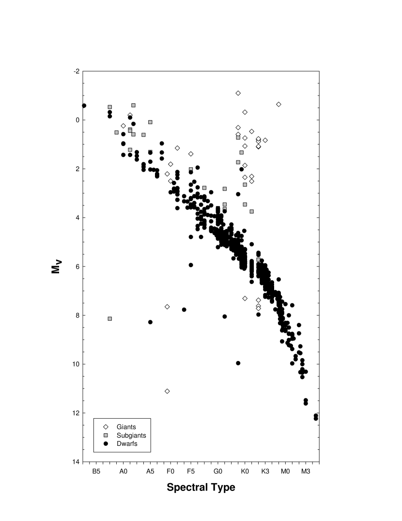
Figure 1: An observational HR diagram formed from the spectral types of the 664 stars reported in this paper. The absolute magnitudes, $M_{v}$, are calculated using Hipparcos (ESA 1997) parallaxes. The stars scattering below the main sequence in this figure all have large parallax errors and are listed in Table 2. These stars are all evidently more distant than 40pc.

Spectral types are important to this project because 1) they provide the first detailed look at our data and enable us to pick out peculiar and astrophysically interesting stars and 2) accurate spectral types yield beginning values for our determination of the basic physical parameters and provide a check on the derived physical parameters. In addition, our spectral types enable us to refine the census of stars within 40pc of the sun. Figure 1 shows an HR diagram based on the spectral types in Table 1 and Hipparcos parallaxes (ESA, 1997). Note the sharp lower edge to the main sequence and the good separation between the luminosity classes. Note, however, the handful of stars scattering below the main sequence. These stars, without exception, have large parallax errors. Most of these stars are in double and multiple systems, explaining the parallax errors. Our spectral types confirm that these stars lie significantly beyond 40pc. These stars are listed in Table 2.

Table 2: Stars Beyond 40 parsecs identified by MK Classification

HIP	BD/HD	Spectral Type	$\pi\pm\sigma_{\pi}$ (mas)	dMK
1663	1651	kA7hA9mF0 III	$46.72\pm 20.16$	290
1692	1690	K2 III	$43.42\pm 33.05$	340
7765	10182	K2 III	$61.30\pm 36.67$	320
24502	33959C	F5 V	$39.77\pm 22.40$	95
30362	256294	B8 IVp	$48.08\pm 13.63$	1050
30756	257498	K0 IIIb	$55.52\pm 33.89$	230
35389	+18 1563	A5 V	$52.47\pm 28.98$	370
76051	+10 2868C	G2 V CH$-$0.3	$44.59\pm 20.41$	90
84581	$-$07 4419B	A9 III	$100.89\pm 43.18$	275
116869	+13 5158B	G8 V+	$44.81\pm 60.22$	80
117042	222788	F3 V	$53.88\pm 32.40$	170

4 Basic Physical Parameters

An important goal of this project is to derive the basic physical parameters - the effective temperature, the surface gravity and the overall metallicity - for as many of our program stars as possible.

4.1 Determination of the Basic Physical Parameters

To determine these parameters, we use a technique similar to that devised by Gray, Graham & Hoyt (2001) which fits the observed spectra and fluxes from medium-band (Strömgren $uvby$) and broad-band (Johnson and Johnson-Cousins $VRI$) photometry, and, when available, IUE spectra, to synthetic spectra and fluxes. The fit is achieved by minimizing a $\chi^{2}$ statistic formed from the point-to-point squared differences between the synthetic and observed spectra plus a similar sum over the squared differences between the observed and synthetic fluxes. The sum of the squared differences for the spectra are given approximately three times the weight of the sum of the squared differences over the fluxes in the final $\chi^{2}$. The synthetic spectra and fluxes are based on Kurucz (1993) atlas9 stellar atmosphere models (calculated without convective overshoot) and the synthetic spectra are computed with the spectral synthesis program spectrum (Gray & Corbally, 1994). Since the publication of the Gray, Graham & Hoyt paper, much effort has been put into improving the spectral line list used by spectrum including updating the oscillator strengths with the latest critically evaluated values from the NIST website. Full details can be found on the spectrum website.

The minimization of the $\chi^{2}$ statistic is carried out by the multidimensional downhill simplex algorithm amoeba (Press et al., 1992). We have modified the Gray, Graham & Hoyt technique by introducing a graphical front end (xfit16) to this algorithm, which allows the user to find visually an approximate global solution which is then polished using the simplex engine. Any of the four basic physical parameters ($T_{\rm eff}$, $\log g$, $\xi_{t}$ – the microturbulent velocity – and [M/H] – the overall metal abundance) may be held fixed or allowed to vary in the solution. A further improvement on the Gray et al. technique is the possibility to introduce observed fluxes not only from Strömgren $uvby$ photometry, but from Johnson and Johnson-Cousins $VRI$ photometry and from IUE spectra. In addition, xfit16 can rotationally broaden the synthetic spectra, and thus is capable of treating even high $v\sin i$ stars. The graphical program xfit16 can access multiple libraries of synthetic spectra for each of the different datasets in the project (for instance, the two dispersions from DSO, spectra from CTIO, the David Dunlap Observatory and the Bok telescope of Steward Observatory). The program xfit16 allows the user not only to verify that the solution obtained is the global solution, but to judge visually the quality of the solution and to decide if any of the input data are defective. While xfit16 allows the user to deredden the observed fluxes, the reddening for all of our program stars was assumed to be zero.

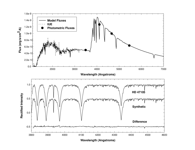
Figure 2: The simplex solution for the early A-type star HD 47105. The top panel shows the fit with respect to photometric fluxes (Strömgren $uvby$) and ultraviolet fluxes from IUE spectra. The bottom panel shows the fit with the observed spectrum; the difference between the observed and synthetic spectrum is seen at the bottom of the panel.

For the B- and early A-type stars in our program, we utilized observed fluxes from the Strömgren $u$, $b$ and $y$ bands and, when available, IUE spectra obtained from the MAST IUE website. The flux calibration used for the Strömgren photometry is that of Gray (1998). Because the metallic lines in these stars are quite weak and thus do not have much leverage on the solution, the solution was first optimized with [M/H] held fixed at 0.00, and then [M/H] was adjusted manually until good agreement was obtained visually with the metallic-line strengths. The solution was then re-optimized and [M/H] readjusted if necessary. For these stars, a microturbulent velocity of 2 km s^-1 was assumed. The IUE spectra, when available, were valuable in determining [M/H] because line blanketing is much greater in the ultraviolet. An example of a simplex/xfit16 solution for an early A-type star, HD 47105, is shown in Figure 2.

For the late A- , F- and early G-type stars IUE spectra were generally not available, and so the flux solution was constrained by fluxes from Strömgren $u$, $b$ and $y$ photometry. For these stars, all four physical parameters were allowed to vary to derive the final solution.

For the late G- and K-type dwarfs, a number of points had to be taken into consideration to achieve good solutions. First, for these cooler stars the flux solution is not well constrained by observed fluxes from the Strömgren bands, but it is necessary to include photometric fluxes from the red and the near infrared in the form of Johnson and/or Johnson-Cousins $VRI$ photometry. We have used the absolute flux calibration for the Cousins $R$ and $I$ bands of Bessell (1990). To ensure uniformity, when only Johnson $VRI$ photometry was available for a star, we used the equations of Fernie (1983) to transform Johnson $V-R$ and $V-I$ colors to Johnson-Cousins $V-R$ and $V-I$ colors and then used Bessell’s calibration. Unfortunately, many of our late G- and K-type stars do not have either Johnson or Johnson-Cousins $VRI$ photometry. We have found, however, that for dwarf stars the following equations are able to predict Johnson-Cousins $V-R$ and $V-I$ colors from Strömgren $b-y$ colors in the range $0.4<b-y<0.8$ with an accuracy of 0.015 magnitude for $V-R$ and 0.03 magnitude for $V-I$.

$$V-R=1.30(b-y)-0.17$$

$$V-I=2.32(b-y)-0.25$$

We can detect only a slight dependence on metallicity in these relationships, well within the errors for stars with [M/H]$>-0.7$. By happy circumstance, most of the very metal-weak stars in our sample have $VRI$ photometry. The Kurucz fluxes in the Strömgren $u$ band do not reproduce well the observed fluxes in the late G- and K-type stars, and so the $u$ band fluxes are not used in the simplex solution for these stars.

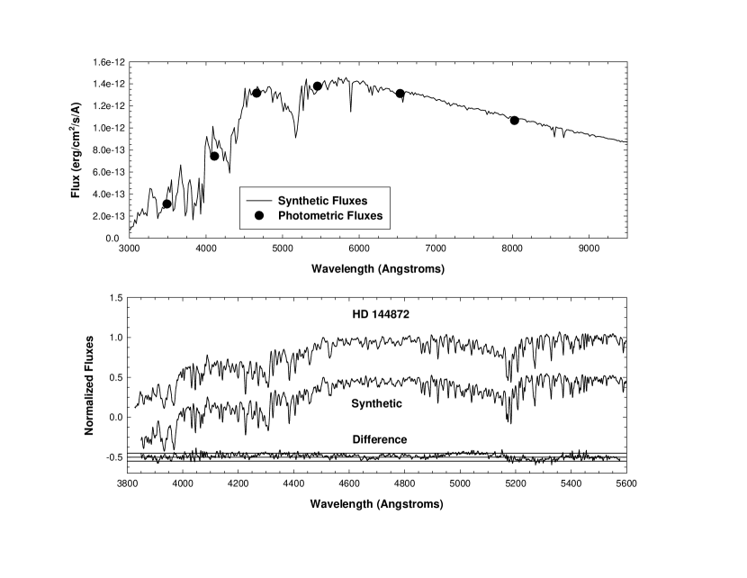
Figure 3: An example of a simplex fit for a K3 dwarf, HD 144872. The difference spectrum (synthetic minus observed) is shown at the bottom of the second panel; the parallel lines indicate errors of $\pm 5$% in the flux. The top panel shows the fit to the observed photometric fluxes; the illustrated points are, from left to right, Strömgren $u$, $v$, $b$ and $y$ fluxes and Johnson-Cousins $R$ and $I$ fluxes. The Strömgren $u$ flux is not used in the solution.

It is unfortunate that neither the energy distributions of the late G- and K-type dwarfs nor our classification spectra strongly constrain the surface gravity for these stars. In the B, A, F and even early G-type stars the Balmer jump strongly constrains the surface gravity, but this feature is too weak to serve this purpose in the late G and K-type stars. The normal MK luminosity criteria in the K-type stars (the strength of the CN band, and certain lines of ionized species such as Sr II $\lambda 4077$ and Y II $\lambda 4376$ – both used in ratio with adjacent Fe I lines) do not offer sufficient leverage in the simplex solutions to yield accurate ($\pm 0.10$ dex) values for $\log g$ in the dwarfs. We have found that allowing $\log g$ to be a free parameter in the simplex solution for the late G- and K-type dwarfs often results in an unreliable (usually too low) value for that parameter in the final solution. We have therefore constrained $\log g$ to the value implied by the Hipparcos parallax and the mass-luminosity relationship (Gorda & Svechnikov, 1998). We have further constrained $\xi_{t}=1.0$km s^-1. With these constraints, we generally obtain good to excellent solutions for dwarfs of spectral type K3 and earlier. An example of such a fit for a K3 dwarf can be seen in Figure 3.

Later than K3, however, the quality of the synthetic spectra and fluxes, especially in the spectral region used (3800 – 5600Å) begins to deteriorate for the dwarf stars. It is clear that in this spectral region, for $T_{\rm eff}<4500$K, a significant contributer to the continuous opacity is missing in both atlas9 and spectrum. Synthetic fluxes normalized and matched in the red to observed fluxes similarly normalized are too high compared to the observed fluxes in the blue-violet, and synthetic line strengths in the blue-violet are too strong. This persists even when both synthetic and observed spectra are normalized at a common point in the blue-violet. This effect is seen even in the NextGen models and synthetic spectra of Hauschildt, Allard & Baron (1999). This missing opacity in the blue-violet region is reminiscent of a similar effect found in K-giant stars in the violet by Short & Lester (1994). Short & Lester suggested this missing violet continuous opacity might be supplied by photodissociation of MgH. However, Weck et al. (2003) have recently calculated this continuous opacity; it is about an order of magnitude too small to explain the observed effect. Other possible culprits include CaH and the O^- ion, as CaH has a dissociation energy similar to that of MgH and the ionization energy of O^- is about 2 eV. This discrepancy between observed and synthetic spectra and fluxes unfortunately prevents us from calculating basic physical parameters for dwarf stars later than K3 from our spectra.

For the late-G and K-type giants and subgiants it is likewise necessary to introduce certain constraints to derive good solutions. For most of the G and K giants and subgiants in our program, $V-K$ photometry exists, and so we have elected to use the Infrared Flux Method (IRFM) of Blackwell & Lynas–Gray (1994) to derive starting conditions and constraints for the simplex solutions. For the few giants without $V-K$ photometry, we have found that the following equations can be used to predict $V-K$ colors to sufficient accuracy ($\pm 0.06$ magnitude) for our purposes:

$$V-K=3.80(b-y)-0.02$$

$$V-K=1.39(B-V)^{2}-0.98(B-V)+1.87$$

valid for $0.55<b-y<0.90$ and $0.90<B-V<1.50$ respectively. The IRFM method uses the following polynomial to predict the effective temperature (for $V-K>0.35$):

$$T_{\rm eff}=8862-2583(V-K)+353.1(V-K)^{2}$$ (1)

The luminosity of the star may be determined using the Hipparcos parallaxes with bolometric corrections (Flower, 1996), and the radius may be determined from the Stefan-Boltzmann law. We then determine the mass for the star using the evolutionary tracks of Claret & Gimenez (1995) for Z = 0.01 (as many of the giants are slightly metal weak) and thence the surface gravity. The normal procedure with the giants is then to constrain the $T_{\rm eff}$ to the IRFM value in the simplex solution, constrain $\xi_{t}=1.0$km s^-1, begin with $\log g$ as calculated above, and [M/H] is manually adjusted so that the line strengths in the synthetic spectrum are approximately correct. The simplex algorithm is then allowed to polish the solution.

The basic physical parameters for this first set of program stars may be found in Table 1.

4.2 Reliability of the Basic Physical Parameters

A thorough discussion of the errors associated with the simplex method may be found in Gray, Graham & Hoyt (2001), but since a number of improvements to both the spectral synthesis program spectrum and to the simplex method have been made since the publication of that paper, a review of the errors is warranted.

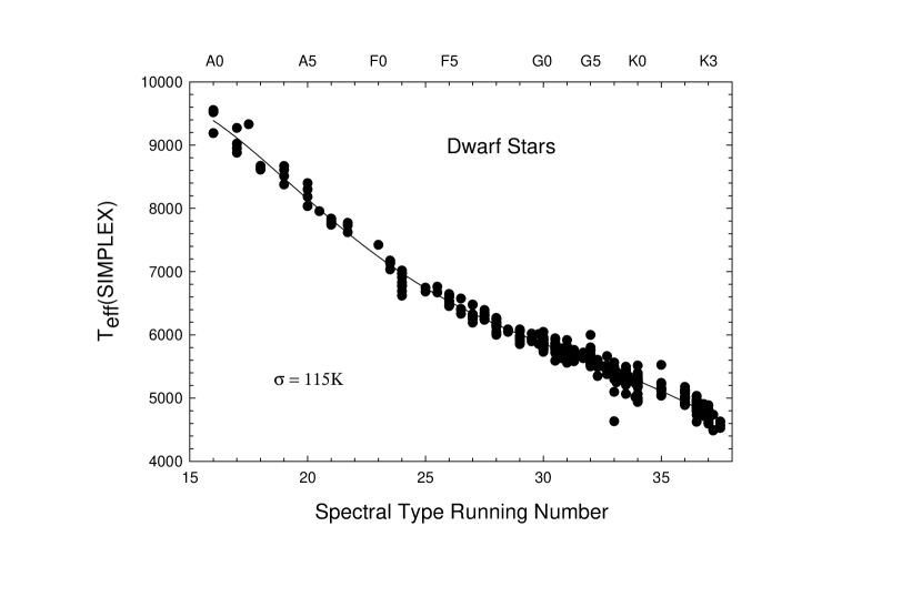
Figure 4: The correlation between the simplex effective temperatures and the spectral type for the dwarf stars in the present sample. The scatter in this relationship is $\pm 115$K and sets an upper limit on the random error in the simplex effective temperatures.

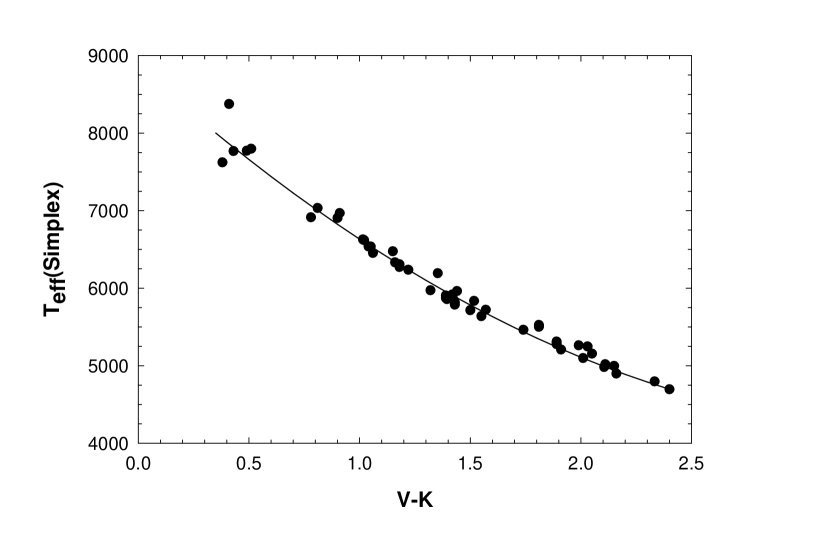
Figure 5: Comparison of simplex effective temperatures with the IRFM calibration. This comparison constitutes an external check on the simplex effective temperatures. The solid line is the IRFM polynomial (equation 1). The scatter of simplex temperatures around this curve is 115K, and the systematic difference over this range of effective temperature does not appear to exceed 30K. The IRFM temperatures are essentially independent of theoretical models.

An excellent internal check on the precision of the simplex effective temperatures is afforded by a comparison with our spectral types. Figure 4 shows a plot of $T_{\rm eff}$ versus the spectral-type running number (Keenan, 1984) for the dwarfs in our sample. A polynomial fit yields a scatter of $\pm 115$K, part of which is attributable to errors in the spectral types and the width of the spectral boxes. This polynomial yields the effective temperature/spectral type calibration for dwarf stars in Table 3. We conservatively estimate a random error in the simplex effective temperatures of $\pm 80$K. For an external check, we may compare the simplex effective temperatures with those derived from the IRFM method (Blackwell & Lynas–Gray, 1994). To do this, we have selected those dwarfs in Table 1 which have $V-K>0.35$ and have plotted (Figure 5) $V-K$ against the simplex effective temperatures. The solid line in that figure shows the IRFM calibration (see equation 1). As can be seen, the agreement is excellent; the scatter around the IRFM calibration is $\pm 115$K and a close comparison suggests that the simplex temperatures are systematically only 30K hotter than the IRFM temperatures.

Table 3: An Effective Temperature Calibration for Dwarf Stars

SpT	$T_{\rm eff}$	SpT	$T_{\rm eff}$	SpT	$T_{\rm eff}$
A2	8800	F3	6740	G5	5580
A3	8480	F5	6530	G8	5430
A5	8150	F7	6250	G9	5350
A7	7830	F8	6170	K0	5280
A9	7380	F9	6010	K1	5110
F0	7240	G0	5860	K2	4940
F1	7100	G1	5790	K3	4750
F2	6980	G2	5720	$\cdots$	$\cdots$

It is of interest to compare the simplex effective temperatures with those in the Cayrel de Strobel, Soubiran & Ralite (2001) catalog (hereinafter the [Fe/H] catalog) which contains determinations of $T_{\rm eff}$, $\log g$ and [Fe/H] from the literature based on high-resolution spectroscopy. This catalog contains only data derived from digital detectors (i.e., older photographic determinations have been removed from this version of the catalog), but the data are not otherwise critically assessed. The [Fe/H] values in this catalog are derived using a number of techniques, ranging from the curve of growth method to spectral synthesis.

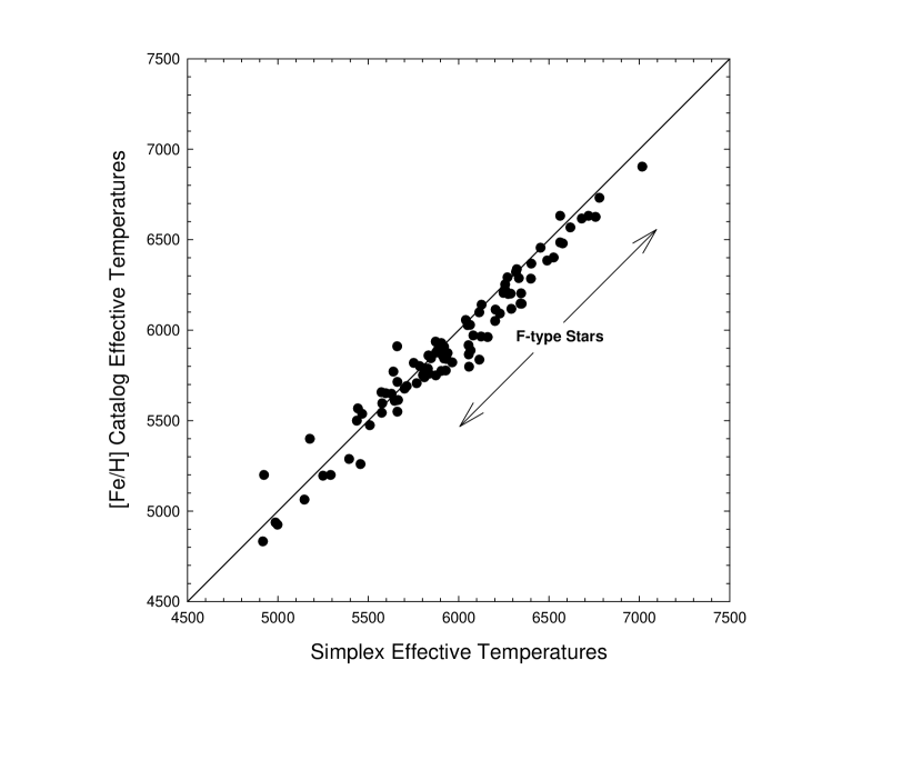
Figure 6: A comparison of the simplex effective temperatures with those in the Cayrel de Strobel, Soubiran & Ralite (2001) [Fe/H] catalog. The systematic difference in the F-type stars is probably due to a defective convective overshoot algorithm used in the published atlas9 models (Kurucz 1993). This has been corrected in the models used in the simplex solutions.

Figure 6 shows that for the G and K-type stars in common there is good agreement between the simplex values of $T_{\rm eff}$ and those of the [Fe/H] catalog ($\sigma=100$K, with a negligible zero-point difference), but in the F-type stars there is a systematic difference in the sense that the simplex effective temperatures are about 100K hotter than the literature values. There is, however, good agreement at G0 and for the early F-type stars.

This systematic difference in the F-type stars can be traced to a faulty convective over-shoot algorithm included in the atlas9 stellar atmosphere program (Kurucz, 1993). This faulty algorithm introduces a systematic error in the structure of the stellar atmosphere models of the partially convective F-type star atmospheres (Smalley & Kupka, 1997). This produces a distortion in the temperature scale of the F-type stars which is unfortunately reflected in many of the determinations listed in the [Fe/H] catalog.

We have recomputed the atlas9 models for the F-type stars with convective overshoot turned off using the implementation of atlas9 by Michael Lemke and used these models in the spectral libraries employed by simplex (see Gray, Graham & Hoyt (2001) for further details).

An important parameter for those who would use our data for the nearby stars in exo-planet searches is the metallicity [M/H] of the star. There is some indication that planets are found preferentially around stars with higher than solar metallicities (Gonzalez, 1999).

Comparing the simplex [M/H] values with mean [Fe/H] values from the [Fe/H] catalog for the stars in common, we find small but significant zero-point differences (see Table 4). The zero-point differences for the dwarfs are generally small, but the zero-point difference for the G and K giants is quite large and requires some discussion. Many of the determinations in the [Fe/H] catalog for G and K-giants were made with stellar atmosphere models calculated with the MARCS code or its predecessors (Gustafsson et al., 1975), and this may possibly indicate a systematic difference between the Kurucz models and the MARCS models. However, we expect that this systematic difference in the giants has more to do with the fact that the abundance determinations in the [Fe/H] catalog were largely carried out at wavelengths $>5000$Å, and for the most part in the red, whereas the simplex solutions use blue-violet spectra (3800 – 5600Å). We have noted above discrepancies in line strengths in the dwarfs between observed and synthetic spectra in the blue-violet for $T_{\rm eff}<4500$K, and we expect that we are seeing a similar phenomenon in the giants, although to a lesser degree (note that many of our giants have $T_{\rm eff}<4500$K). Missing continuous opacity in the blue-violet would lead to greater line strengths in the models, and thus systematically negative values for [M/H].

Table 4: Zeropoint Differences: [Fe/H]${}_{\rm catalog}-$[M/H]_simplex

Stellar Type	Resolution	Zeropoint
F & G dwarfs	1.8 Å	0.02
G & K dwarfs	3.6 Å	0.05
G & K giants	3.6 Å	0.23

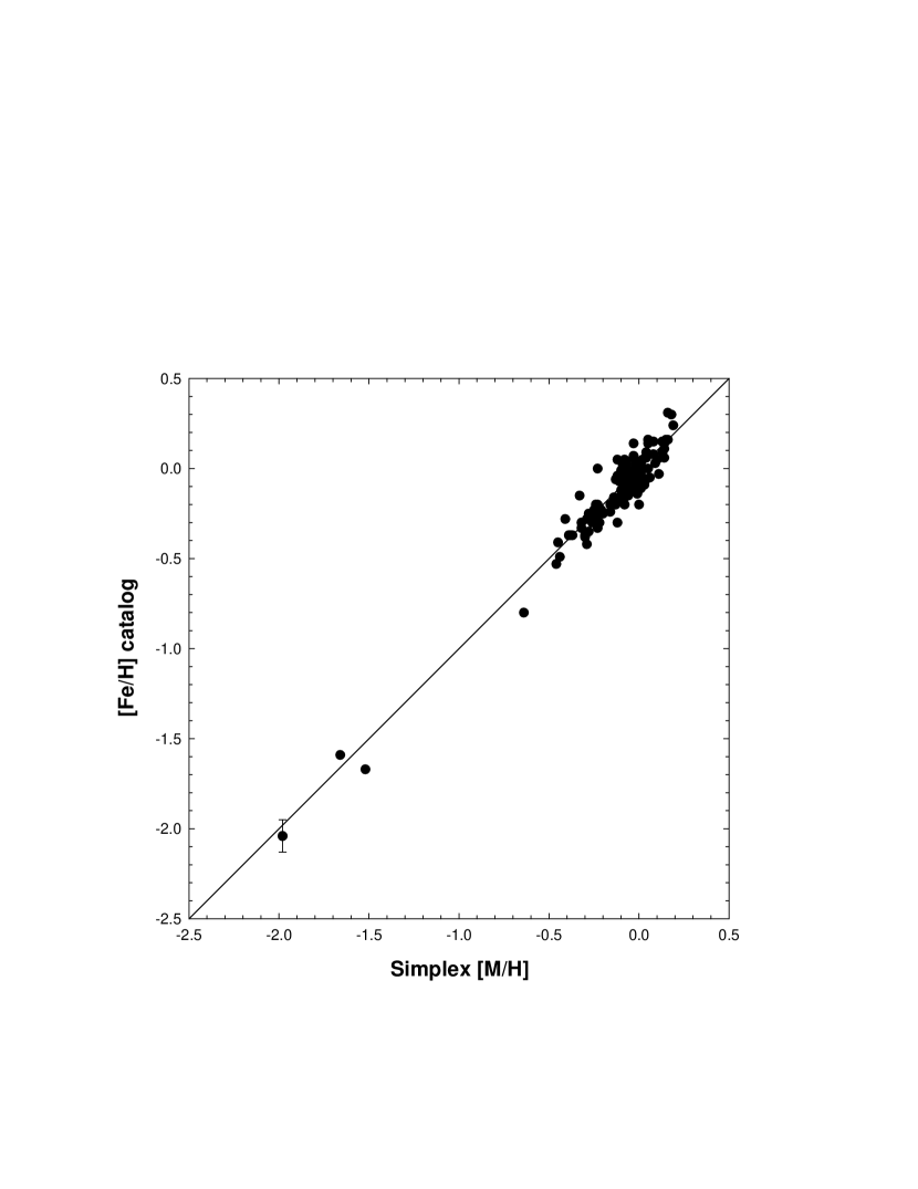
Figure 8: A comparison between the simplex [M/H] (overall metal abundance) and mean [Fe/H] values from the Cayrel de Strobel, Soubiran & Ralite (2001) [Fe/H] catalog. The scatter in the comparison is 0.09 dex, similar to the scatter for single stars in the [Fe/H] catalog, $\approx 0.08$ dex.

Having applied the zero-point corrections in Table 4 to the simplex [M/H] values, we find excellent agreement with the [Fe/H] catalog values (see Figure 8). The [M/H] values in Table 1 have had these corrections applied. The random error in the comparison is only $\pm 0.09$ dex, hardly larger than the internal scatter in the [Fe/H] catalog ($\approx 0.08$ dex, illustrated with error bars on one point in the figure). This is an impressive result, considering that the [Fe/H] catalog values were determined from high resolution spectra. Such accurate and homogeneous [M/H] values for a large sample of nearby stars will make possible a number of investigations, including examination of the hypothesis that planets are found preferentially around metal-rich stars. We will consider this hypothesis in paper II of this series.

5 Chromospheric Emission

All of the spectra obtained for this project include the Ca II K & H lines and thus can be used to obtain measures of the chromospheric emission, as emission from the chromosphere can be detected in the cores of these very strong lines. This is an important measurement, as chromospheric emission can be an indication of the age of a star and/or its binary status. An age determination can be important for exo-planet searches, as an indication of a young age for a star might preclude observations using interferometric or coronographic techniques due to the complicating effects of zodiacal light from a remnant protoplanetary disk.

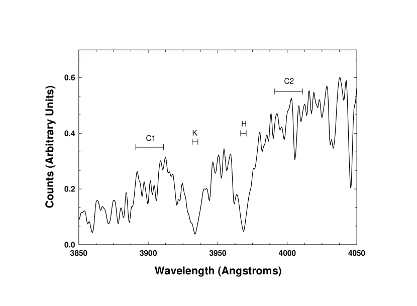
Figure 9: Numerical passbands utilized in the calculation of the chromospheric activity index $S$. Two bands, each 4Å wide, are centered on the Ca II K & H lines. The $C_{1}$ and $C_{2}$ bands measure the flux in the continuum in 20Å-wide segments of the spectrum on either side of the K & H lines.

We measure the chromospheric emission in our program stars by calculating relative fluxes in four wavelength bands (see Figure 9), two of which are centered on the Ca II K & H lines. The other two bands measure fluxes in the “continuum” just shortwards and longwards of Ca II K & H. These bands are essentially identical to those used in the Mount Wilson chromospheric activity survey program (Baliunas et al., 1995) except that the bands centered on Ca II K & H are wider (4 Å) than those used at Mount Wilson (1 Å) because our spectra are of lower resolution. Our instrumental chromospheric emission index is calculated, like the Mount Wilson index, with the following equation:

$$S=5\frac{K+H}{C_{1}+C_{2}}$$

This index is defined in such a way that it is insensitive to the local slope of the continuum in the vicinity of the Ca II K & H lines. Thus, we find that this index is identical (within a few thousandths) whether we use flux-calibrated spectra or uncalibrated raw counts. We determine this index by using a feature in the spectral classification program xmk19 that allows the user to shift the spectrum in wavelength to exactly align the $K$ and $H$ bands with the cores of the Ca II K & H lines and which then carries out a numerical integration over the four bands. To ensure accuracy in the numerical integration over these bands, we resample the spectrum into 0.1 Å bins.

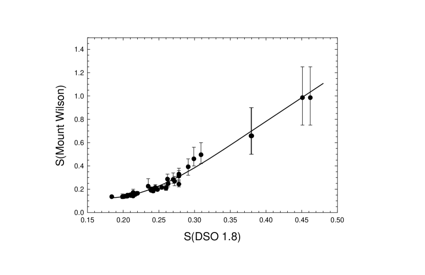
Figure 10: The calibration between the instrumental $S_{18}$ chromospheric activity index and the Mount Wilson $S$ index. The “error bars” represent the range of variation shown by the star in Baliunas et al. (1995). The solid line shows the adopted calibration.

To place this chromospheric index on the Mount Wilson scale, it is necessary to use “standard” stars to derive a transformation equation. Unfortunately, all solar-type stars show some variability in the chromospheric index, and those with higher values of $S$ are generally more variable. What this means is that unless one has observations taken near in time to Mount Wilson observations, it is impossible to derive an exact transformation equation. One, however, can derive a transformation of sufficient accuracy to characterize stars as active, inactive, etc. by selecting from the Mount Wilson list (Baliunas et al., 1995) those stars that do not show long-term secular trends or irregular behavior as calibration stars. The stars we have selected for this purpose are listed in Table 5. The resulting calibration for the 1.8 Å resolution spectra is shown in Figure 10. To fit the trend in Figure 10, we have employed a cubic fit given by the following equation:

$$S_{\rm MW}=-39.976S_{18}^{3}+43.335S_{18}^{2}-11.592S_{18}+1.041$$

for $S_{18}<0.361$. For $S_{18}\geq 0.361$ (the inflection point of the above cubic), the curve is extended with a straight line, having the slope of the cubic at the inflection point:

$$S_{\rm MW}=4.067S_{18}-0.845$$

This straight line is also used to extrapolate to values of $S_{\rm MW}$ outside the range represented by the calibration stars.

We estimate the errors in this transformation allow a determination of the Mount Wilson activity index, $S_{\rm MW}$, to an accuracy of 5% with larger uncertainties (including unknown systematic errors) for $S_{\rm MW}>0.8$. To ensure compatibility of the derived $S_{\rm MW}$ values from the 3.6 Å resolution spectra with the 1.8Å spectra, we first transform the instrumental $S_{36}$ values onto the instrumental $S_{18}$ system and then use the above calibration. The transformation from the $S_{36}$ system to the $S_{18}$ system is determined by using stars observed with both resolutions within a time frame of a few months. This transformation is linear, with a slope of unity and a zeropoint difference of 0.039. The scatter in this transformation, an indication of the precision with which we can measure $S_{\rm MW}$, is $\pm 0.010$.

Table 5: Chromospheric Activity Calibration Stars

HD	$<S_{\rm MW}>$	HD	$<S_{\rm MW}>$
9562	0.136	131156A	0.461
16160	0.226	136202	0.140
16673	0.215	141004	0.155
18256	0.185	142373	0.147
22049	0.496	143761	0.150
26923	0.287	152391	0.393
29645	0.140	154417	0.269
33608	0.214	158614	0.158
43587	0.156	159332	0.144
45067	0.141	178428	0.154
78366	0.248	182101	0.216
81809	0.172	187013	0.154
82885	0.284	188512	0.136
89744	0.137	190360	0.146
100180	0.165	194012	0.198
100563	0.202	201091	0.658
106516	0.208	201092	0.986
114378	0.244	206860	0.330
114710	0.201	212754	0.140
115383	0.313	216385	0.142
120136	0.191	217014	0.149
126053	0.165	$\cdots$	$\cdots$

The $S_{\rm MW}$ index measures the flux in the core of the Ca II K & H lines, but there are both photospheric and chromospheric contributions to this flux. The photospheric flux may be removed approximately following the procedure of Noyes et al. (1984) who derive a quantity $R_{\rm HK}\propto F_{\rm HK}/\sigma T_{\rm eff}^{4}$ where $F_{\rm HK}$ is the flux per cm^-2 in the H and K bandpasses. $R_{\rm HK}$ can be derived from $S_{\rm MW}$ by modeling the variation in the continuum fluxes (in bands C₁ and C₂) as a function of effective temperature (using $B-V$ as a proxy). $R_{\rm HK}$ must then be further corrected by subtracting off the photospheric contribution in the cores of the H & K lines. The logarithm of the final quantity, $R^{\prime}_{\rm HK}$ is then a useful measure of the chromospheric emission, essentially independent of the effective temperature. We have calculated $R^{\prime}_{\rm HK}$ for all of our dwarf program stars later than F5 and earlier than M0 with $B-V$ photometry. While the conversion of $S_{\rm MW}$ into $R^{\prime}_{\rm HK}$ becomes increasingly uncertain for $B-V>1.20$ (approximately spectral type K5), we have carried this calculation out for stars as late as K8. Both the $S_{\rm MW}$ and the $\log R^{\prime}_{\rm HK}$ indices are tablulated for our program stars in Table 1.

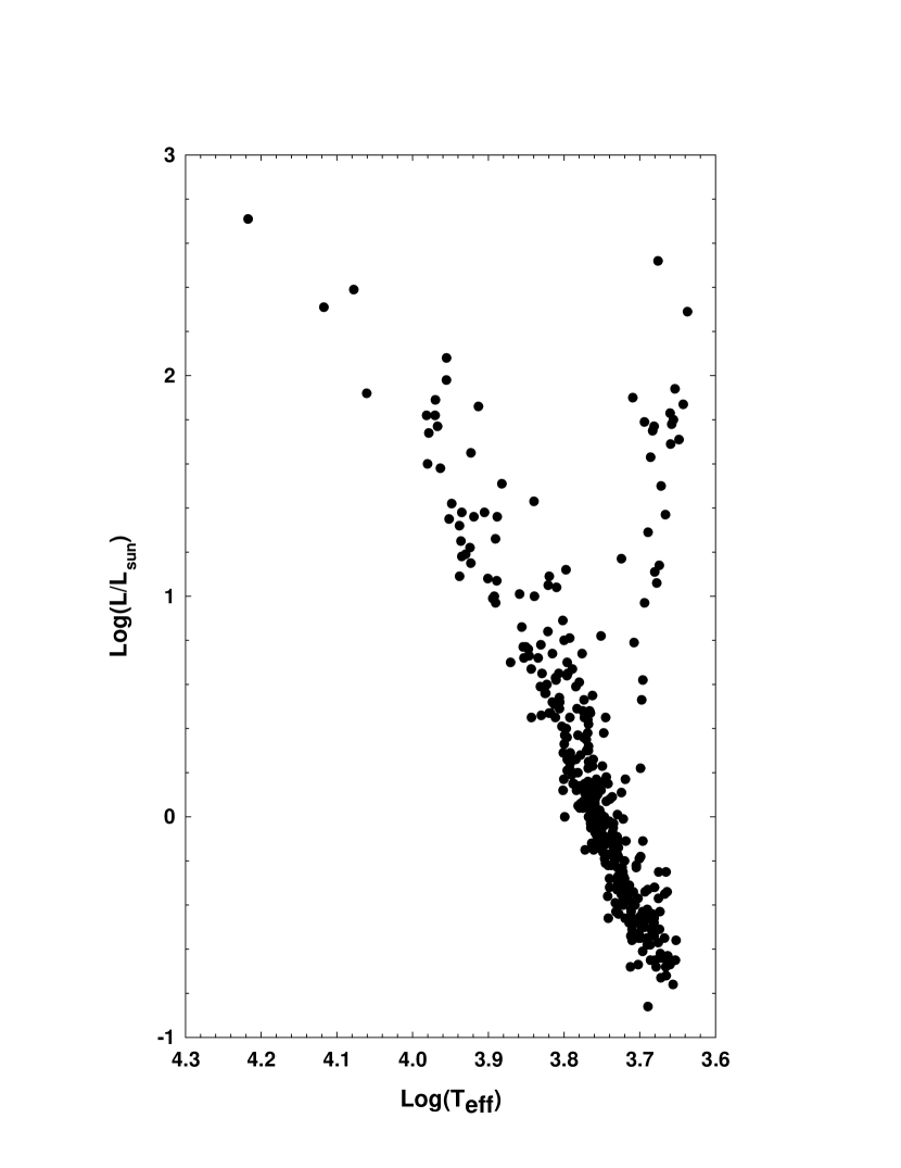
Figure 7: An astrophysical HR diagram based on simplex physical parameters.

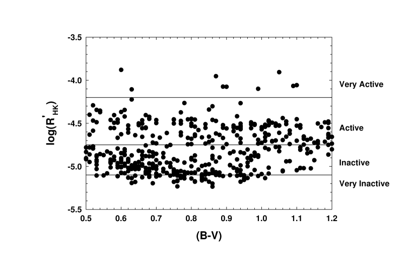
Figure 11: A plot of the chromospheric flux parameter $\log R^{\prime}_{\rm HK}$ versus the $B-V$ color. This diagram allows the classification of stars into the chromospheric activity categories “Very Inactive”, “Inactive”, “Active” and “Very Active”. All but one of the “Very Active” stars are well-known flare, BY Dra or RS CVn variables. The exception is HIP 90035 (see text and figure 13).

We follow Henry et al. (1996) in employing $\log R^{\prime}_{\rm HK}$ to classify stars into “Very Inactive”, “Inactive”, “Active” and “Very Active” categories (see Figure 11 and Table 1). The distribution of stars in Figure 11 is similar to that in Figure 7 of Henry et al., except that their study had a bias toward G-dwarfs and did not go to as late a spectral type as our project.

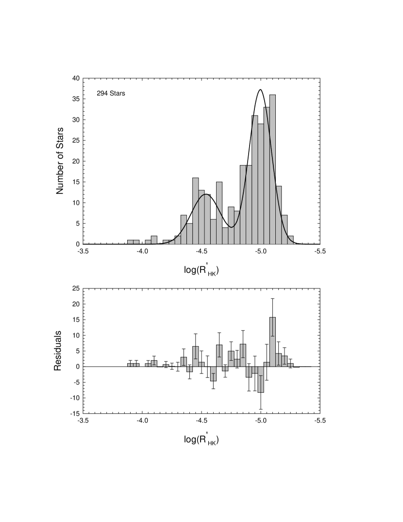
Figure 12: The distribution of the chromospheric flux parameter $\log R^{\prime}_{\rm HK}$ for stars with $0.50<B-V<0.90$. The distribution is clearly bimodal, with the main peak representing chromospherically inactive stars, and the secondary peak chromospherically active stars. The double Gaussian curve is a fit to the distribution. The lower panel shows the residuals associated with this fit. With the exception of the bin centered at $\log R^{\prime}_{\rm HK}=-5.1$, the fit is within the errors. The excess number of stars at $\log R^{\prime}_{\rm HK}=-5.1$ is discussed in §5.

Figure 12 shows a histogram of the $\log R^{\prime}_{\rm HK}$ values for the program stars with $0.5<B-V<0.9$. This distribution may be compared directly with Figure 8 of Henry et al. It is clear that the distribution is bimodal, with a peak near $\log R^{\prime}_{\rm HK}=-5.0$ and another peak near $-4.5$, very similar to that found by Henry et al. We have used the Levenberg-Marquardt method (Press et al., 1992) to fit a double-Gaussian model to this distribution; the result is shown in Figure 12 with the residuals from the fit illustrated in the lower panel. It is clear that this double Gaussian-model (peaks at $\log R^{\prime}_{\rm HK}=-4.996$ and $-4.536$, with FWHM = 0.266 and 0.352 respectively – again very similar to the results of Henry et al.) fits the distribution within the errors, with the possible exception of one bin, at $\log R^{\prime}_{\rm HK}=-5.1$. This bin shows an excess (a 2.5$\sigma$ result) of stars. An examination of Table 1 shows that out of the 36 stars in this bin, only 2 are metal-weak ([M/H]$<-0.50$) and 3 are slightly evolved (either classified as subgiants or having $\log g<=4.00$). The remaining stars in this bin are apparently normal, near-solar metallicity, chromospherically-inactive dwarfs. This result suggests that the excess stars in this bin and in all the bins representing very inactive stars ($\log R^{\prime}_{\rm HK}<-5.1$) may be due to dwarfs in a Maunder-minimum phase (see as well Henry et al. 1996, and Table 6 for a list of possible solar-metallicity Maunder-minimum dwarfs). However, as these excesses are only marginally significant statistically with the current sample, we will defer discussion of this point to later papers in this series.

Table 6: Possible Solar-Metallicity Maunder-Minimum Dwarfs

HIP	BD/HD	Spectral Type	[M/H]	$\log R^{\prime}_{\rm HK}$
9269	12051	G9 V	0.00	-5.134
35872	57901	K3- V	0.00	-5.135
39064	65430	K0 V	-0.20	-5.110
42499	73667	K2 V	-0.15	-5.127
67246	120066	G0 V	0.14	-5.193
70873	127334	G5 V CH+0.3	-0.03	-5.118
88348	164922	G9 V	0.00	-5.141
101345	195564	G2 V	-0.09	-5.196
116085	221354	K0 V	0.00	-5.149

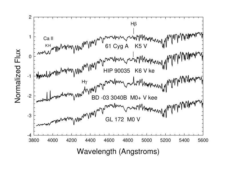
Figure 13: HIP 90035 = BD+01 3657 is a chromospherically very active star which has not been classified as a flare, BY Dra or RS CVn star. Note the strong emission (in comparison with the K5 V standard 61 Cyg A) in Ca II K & H lines, and the infilling of the H$\beta$ line with emission. Likewise, BD $-$03 3040B is a chromospherically active early-M dwarf, not yet classified in the literature as an emission-line star, showing strong emission in Ca II K & H as well as H$\beta$, H$\gamma$ and H$\delta$.

Most of the stars in the “very active” category in Figure 11 are well-known variables of either the BY Dra or RS CVn types. These stars are named in the notes to Table 1 (§6). Two exceptions are HIP 90035 = BD+01 3657 which shows strong emission in Ca II K & H, but which is not a known variable and BD$-$03 3040B which shows strong emission in Ca II and the hydrogen lines. See the notes in §6 and Figure 13.

6 Notes on Astrophysically Interesting Stars

HIP 7585 = HD 9986: Solar twin. Notice how closely the simplex basic physical parameters resemble those of the sun. This star is also chromospherically inactive, and has a classification spectrum indistinguishable from that of the sun. However, in a speckle survey of G-dwarfs (Horch et al., 2002), this star, while not resolved, was listed as a suspected non-single star.
HIP 16209 = LHS 173: This star is clearly metal-weak, but abundance-independent criteria place the spectral type of this star near to K7. At that spectral type the MgH band at $\lambda 4780$ appears of nearly normal strength. This luminosity (gravity) sensitive feature therefore suggests an unusually high gravity. Classified as a subdwarf K7 star by Gizis (1997).
HIP 53910 = HD 95418: Some sharp lines, Fe II 4233 enhanced. May be mild shell star.
BD$-$03 3040B: strong emission in Ca II H & K and the hydrogen lines. This star is not a known variable, but has been detected in the X-ray by ROSAT (Mason et al., 1995). Observed on Jan 31, 2001. Double with HD 96064. HD 96064 is as well chromospherically active suggesting that this is a young binary system. See Figure 13.
HIP 90035 = BD+01 3657: Very active chromospherically, but is not a known variable. Observed on Aug 8, 2000. Detected in the extreme ultraviolet (Lampton et al., 1997). A probable new BY Dra variable. See Figure 13.

7 Conclusions

We have presented a database for 664 dwarf and giant stars earlier than M0 within 40pc of the sun that includes new, homogeneous spectral types, basic physical parameters and measures of chromospheric activity. Similar data on the remaining 2935 solar-type nearby stars will be presented in subsequent papers in this series. The goals of this project are to characterize the stellar population in the solar neighborhood and to provide data which will be useful in the selection of targets for the Space Interferometry Mission and the Terrestrial Planet Finder Mission. As an example of how this database could be helpful in selection of targets for discovering terrestrial planets around solar-type stars, the following table (Table 7) contains stars from the database that satisfy the following criteria:

1. Solar-type dwarfs with spectral types from F8 – G8.

2. Solar metallicity: [M/H]$>-0.10$ (following the hypothesis of Gonzalez (1999) that planets are found preferentially around metal-rich stars – the validity of this hypothesis will be tested in paper II).

3. Chromospherically inactive or very inactive: chromospheric activity can be an indicator of a young age; to find terrestrial planets with extraterrestrial life, older stars should be selected. In addition, a young age for the star might preclude observation by a spacecraft like the TPF because of the presence of excessive zodiacal light in the system.

4. Single and non-variable.

It should be noted that 13 of the stars in Table 1 already have known planets. These are HD 19994, 46375, 75732, 89744, 137759, 143761, 145675, 186427, 190360, 210277, 217014, 217107 and 222404. These stars have not been included in Table 7.

Table 7: Candidate Stars for Terrestrial Planet Surveys

HIP	BD/HD	Spectral Type
1499	1461	G3 V
7585	9986	G2 V
7918	10307	G1 V
14150	18803	G6 V
14632	19373	F9.5 V
14954	19994	F8.5 V
24813	34411	G1 V
30545	45067	F8 V
41484	71148	G1 V
49081	86728	G4 V
49756	88072	G3 V
56242	100180	F9.5 V
61053	108954	F9 V
67246	120066	G0 V
70873	127334	G5 V CH+0.3
73100	132254	F8- V
74605	136064	F8 V
79862	147044	G0 V
85042	157347	G3 V
85810	159222	G1 V
89474	168009	G1 V
90864	171067	G6 V
94981	181655	G5 V
96895	186408	G1.5 V
100017	193664	G0 V
101345	195564	G2 V
102040	197076	G1 V
103682	199960	G1 V

The data presented in this paper are currently available on the project’s website and work is continuing on the remaining stars in the project which will be the subject of future papers in this series. As more results become available and the statistical significance of our results improve, we intend to examine detailed features of the distribution of chromospheric activity among solar-type stars, the validity of the hypothesis that exoplanets are found preferentially around metal-rich stars and to point out stars of astrophysical interest and of interest to the SIM and TPF missions.

Table 7: Spectral Types, Basic Physical Parameters and Chromospheric Indices

HIP	BD/HD	SpT	N1	$T_{\rm eff}$	$\log g$	$\xi_{t}$	$[M/H]$	N2	SMW	$\log(R^{\prime})$	AC	N3
171	224930	G5 V Fe$-$1	$\cdots$	5502	4.27	(1.0)	$-$0.64	$\cdots$	0.183	$-$4.880	I	1.8
400	225261	G9 V	$\cdots$	5250	4.40	(1.0)	$-$0.43	$\cdots$	0.148	$-$5.094	I	3.6
518	123	G4 V	*	5718	4.50	(1.0)	0.06	$\cdots$	0.257	$-$4.644	A	1.8
544	166	G8 V	$\cdots$	5412	4.41	(1.0)	0.07	$\cdots$	0.379	$-$4.458	A	3.6
677	358	B8 IV-V Hg Mn	$\cdots$	13098	3.91	(2.0)	(0.0)	*	$\cdots$	$\cdots$	$\cdots$	$\cdots$
746	432	F2 III	$\cdots$	6915	3.49	3.1	$-$0.02	$\cdots$	$\cdots$	$\cdots$	$\cdots$	$\cdots$
974	+26 8	K3 V	$\cdots$	$\cdots$	$\cdots$	$\cdots$	$\cdots$	$\cdots$	0.392	$-$4.775	I	3.6
1499	1461	G3 V	$\cdots$	5700	4.31	(1.0)	0.07	$\cdots$	0.151	$-$5.059	I	1.8
1532	$-$10 47	M0 V	$\cdots$	$\cdots$	$\cdots$	$\cdots$	$\cdots$	$\cdots$	$\cdots$	$\cdots$	$\cdots$	$\cdots$
1598	1562	G1 V	$\cdots$	5756	4.43	(1.0)	$-$0.22	$\cdots$	0.162	$-$4.979	I	1.8
1663	1651	kA7hA9mF0 III	$\cdots$	$\cdots$	$\cdots$	$\cdots$	$\cdots$	$\cdots$	$\cdots$	$\cdots$	$\cdots$	$\cdots$
1692	1690	K2 III	$\cdots$	$\cdots$	$\cdots$	$\cdots$	$\cdots$	$\cdots$	$\cdots$	$\cdots$	$\cdots$	$\cdots$
1860	$\cdots$ B	M2.5 V	$\cdots$	$\cdots$	$\cdots$	$\cdots$	$\cdots$	$\cdots$	$\cdots$	$\cdots$	$\cdots$	$\cdots$
2762	3196	F8.5 V	*	6067	4.35	1.9	$-$0.13	$\cdots$	0.301	$-$4.461	A	1.8
3092	3627	K3 III	$\cdots$	4392	1.87	(1.0)	$-$0.03	K	$\cdots$	$\cdots$	$\cdots$	$\cdots$
3093	3651	K0 V	$\cdots$	5280	(4.43)	(1.0)	0.09	$\cdots$	0.153	$-$5.087	I	1.8
3203	3821	G1 V (k)	$\cdots$	5785	4.40	(1.0)	$-$0.07	$\cdots$	0.287	$-$4.525	A	1.8
3206	3765	K2.5 V	$\cdots$	4892	(4.36)	(1.0)	$-$0.11	$\cdots$	0.161	$-$5.101	VI	3.6
3418	+33 99	K5$-$ V	$\cdots$	$\cdots$	$\cdots$	$\cdots$	$\cdots$	$\cdots$	0.452	$-$4.848	I	3.6
3535	4256	K3 IV-V	$\cdots$	4801	(4.43)	(1.0)	0.00	$\cdots$	0.192	$-$5.042	I	3.6
3757	$\cdots$ B	M2.5 V	$\cdots$	$\cdots$	$\cdots$	$\cdots$	$\cdots$	$\cdots$	$\cdots$	$\cdots$	$\cdots$	$\cdots$
3765	4628	K2 V	$\cdots$	4998	(4.66)	(1.0)	$-$0.43	$\cdots$	0.159	$-$5.071	I	3.6
3810	4676	F8 V	$\cdots$	6254	4.38	1.7	$-$0.03	$\cdots$	0.158	$-$4.917	I	1.8
3876	4635	K2.5 V+	$\cdots$	$\cdots$	$\cdots$	$\cdots$	$\cdots$	$\cdots$	0.292	$-$4.742	A	3.6
3909	4813 B	F7 V	$\cdots$	6250	4.28	1.4	$-$0.06	$\cdots$	0.183	$-$4.780	I	1.8
3937	$\cdots$ B	M3 V kee	$\cdots$	$\cdots$	$\cdots$	$\cdots$	$\cdots$	$\cdots$	$\cdots$	$\cdots$	$\cdots$	$\cdots$
3979	4915	G6 V	$\cdots$	5608	4.51	(1.0)	$-$0.24	$\cdots$	0.175	$-$4.915	I	3.6
3998	4913	K6$-$ V	$\cdots$	$\cdots$	$\cdots$	$\cdots$	$\cdots$	$\cdots$	0.704	$-$4.750	I	3.6
4454	5351	K4 V	$\cdots$	$\cdots$	$\cdots$	$\cdots$	$\cdots$	$\cdots$	0.222	$-$5.015	I	3.6
4845	$-$11 192	M0 V	$\cdots$	$\cdots$	$\cdots$	$\cdots$	$\cdots$	$\cdots$	$\cdots$	$\cdots$	$\cdots$	$\cdots$
4849	6101	K3 V	$\cdots$	$\cdots$	$\cdots$	$\cdots$	$\cdots$	$\cdots$	0.458	$-$4.661	A	3.6
4872	+61 195	M2+ V	$\cdots$	$\cdots$	$\cdots$	$\cdots$	$\cdots$	$\cdots$	$\cdots$	$\cdots$	$\cdots$	$\cdots$
4907	5996	G9 V (k)	$\cdots$	5497	4.50	(1.0)	$-$0.14	$\cdots$	0.382	$-$4.454	A	1.8
5110	6440	K3.5 V	$\cdots$	$\cdots$	$\cdots$	$\cdots$	$\cdots$	$\cdots$	0.649	$-$4.802	I	3.6
$\cdots$	6440B	K8 V	$\cdots$	$\cdots$	$\cdots$	$\cdots$	$\cdots$	$\cdots$	1.623	$\cdots$		3.6
5247	+63 137	K7 V	$\cdots$	$\cdots$	$\cdots$	$\cdots$	$\cdots$	$\cdots$	0.912	$-$4.801	I	3.6
5286	6660	K4 V	$\cdots$	$\cdots$	$\cdots$	$\cdots$	$\cdots$	$\cdots$	0.549	$-$4.747	A	3.6
5336	6582	K1 V Fe$-$2	$\cdots$	5526	(4.49)	(1.0)	$-$0.77	$\cdots$	0.157	$-$5.031	I	3.6
5521	6963	G7 V	$\cdots$	$\cdots$	$\cdots$	$\cdots$	$\cdots$	$\cdots$	0.222	$-$4.768	I	3.6
5799	7439	F5 V	$\cdots$	6465	3.99	1.5	$-$0.22	$\cdots$	0.181	$-$4.754	I	1.8
5944	7590	G0$-$ V (k)	$\cdots$	6013	4.62	1.9	$-$0.16	$\cdots$	0.294	$-$4.487	A	1.8
5957	$\cdots$ B	M0 V	$\cdots$	$\cdots$	$\cdots$	$\cdots$	$\cdots$	$\cdots$	$\cdots$	$\cdots$	$\cdots$	$\cdots$
6405	8262	G2 V	$\cdots$	5821	4.34	(1.0)	$-$0.13	$\cdots$	0.154	$-$5.030	I	1.8
6706	8723	F2 V	$\cdots$	6690	4.12	1.6	$-$0.26	$\cdots$	$\cdots$	$\cdots$	$\cdots$	$\cdots$
6917	8997	K2.5 V	$\cdots$	4793	(4.41)	(1.0)	$-$0.56	$\cdots$	0.509	$-$4.557	A	3.6
7339	9407	G6.5 V	$\cdots$	$\cdots$	$\cdots$	$\cdots$	$\cdots$	$\cdots$	0.158	$-$5.021	I	3.6
7576	10008	G9 V k	$\cdots$	5272	4.50	(1.0)	$-$0.03	$\cdots$	0.361	$-$4.530	A	3.6
7585	9986	G2 V	*	5749	4.39	(1.0)	$-$0.03	$\cdots$	0.168	$-$4.949	I	1.8
7646	$\cdots$ B	M2.5 V	$\cdots$	$\cdots$	$\cdots$	$\cdots$	$\cdots$	$\cdots$	$\cdots$	$\cdots$	$\cdots$	$\cdots$
7734	10086	G5 V	$\cdots$	5659	4.61	(1.0)	$-$0.02	$\cdots$	0.228	$-$4.723	A	1.8
7762	+14 253	K4.5 V	*	$\cdots$	$\cdots$	$\cdots$	$\cdots$	$\cdots$	$\cdots$	$\cdots$	$\cdots$	$\cdots$
7765	10182	K2 III	*	$\cdots$	$\cdots$	$\cdots$	$\cdots$	$\cdots$	$\cdots$	$\cdots$	$\cdots$	$\cdots$
7918	10307	G1 V	$\cdots$	5874	4.35	(1.0)	0.10	$\cdots$	0.155	$-$5.017	I	1.8
7981	10476	K0 V	$\cdots$	5249	(4.55)	(1.0)	$-$0.13	$\cdots$	0.151	$-$5.095	I	3.6
8043	+27 273	M1 V	$\cdots$	$\cdots$	$\cdots$	$\cdots$	$\cdots$	$\cdots$	$\cdots$	$\cdots$	$\cdots$	$\cdots$
8070	10436	K5.5 V	$\cdots$	$\cdots$	$\cdots$	$\cdots$	$\cdots$	$\cdots$	0.905	$-$4.657	A	3.6
8275	10853	K3.5 V	$\cdots$	4529	(4.74)	(1.0)	$-$0.74	$\cdots$	0.718	$-$4.503	A	3.6
8362	10780	G9 V	$\cdots$	5312	4.38	(1.0)	0.07	$\cdots$	0.186	$-$4.933	I	3.6
$\cdots$	+63 241	K5 Ib	*	$\cdots$	$\cdots$	$\cdots$	$\cdots$	$\cdots$	$\cdots$	$\cdots$	$\cdots$	$\cdots$
8486	11131	G1 V (k)	$\cdots$	5819	4.53	(1.0)	$-$0.02	$\cdots$	0.298	$-$4.521	A	1.8
8497	11171	F2 III-IV	$\cdots$	7087	4.10	2.4	0.15	$\cdots$	$\cdots$	$\cdots$	$\cdots$	$\cdots$
8543	11130	G9 V	$\cdots$	5270	4.65	(1.0)	$-$0.57	$\cdots$	0.138	$-$5.165	VI	3.6
8796	11443	F6 IV	$\cdots$	6273	3.57	2.1	$-$0.24	*	$\cdots$	$\cdots$	$\cdots$	$\cdots$
8867	11373	K3 V k	$\cdots$	4666	(4.63)	(1.0)	$-$0.45	$\cdots$	0.630	$-$4.516	A	3.6
8903	11636	kA4hA5mA5 Va	$\cdots$	8300	4.10	3.5	0.02	$\cdots$	$\cdots$	$\cdots$	$\cdots$	$\cdots$
9269	12051	G9 V	$\cdots$	5446	4.36	(1.0)	0.00	$\cdots$	0.142	$-$5.134	VI	1.8
9829	12846	G2 V$-$	$\cdots$	5667	4.38	(1.0)	$-$0.25	$\cdots$	0.164	$-$4.975	I	1.8
9884	12929	K1 IIIb	$\cdots$	4504	2.20	(1.0)	$-$0.33	K	$\cdots$	$\cdots$	$\cdots$	$\cdots$
10064	13161	A5 IV	$\cdots$	8186	3.70	(2.0)	0.20	*	$\cdots$	$\cdots$	$\cdots$	$\cdots$
10321	13507	G5 V	$\cdots$	5569	4.35	(1.0)	$-$0.19	$\cdots$	0.292	$-$4.548	A	1.8
10339	13531	G7 V	$\cdots$	5517	4.48	(1.0)	$-$0.08	$\cdots$	0.329	$-$4.497	A	3.6
10416	13789	K3.5 V	$\cdots$	$\cdots$	$\cdots$	$\cdots$	$\cdots$	$\cdots$	0.704	$-$4.527	A	3.6
10505	13825	G5 IV-V	$\cdots$	5550	4.10	(1.0)	0.12	$\cdots$	0.164	$-$4.986	I	3.6
10723	14214	G0 IV$-$	$\cdots$	5958	3.98	1.6	0.01	$\cdots$	0.140	$-$5.114	VI	1.8
11000	14635	K4$-$ V	$\cdots$	$\cdots$	$\cdots$	$\cdots$	$\cdots$	$\cdots$	0.687	$-$4.584	A	3.6
11452	15285	M1 V	$\cdots$	$\cdots$	$\cdots$	$\cdots$	$\cdots$	$\cdots$	$\cdots$	$\cdots$	$\cdots$	$\cdots$
12114	16160	K3 V	$\cdots$	4739	(4.58)	(1.0)	$-$0.37	$\cdots$	0.170	$-$5.094	I	3.6
12158	16287	K2.5 V (k)	$\cdots$	4917	(4.50)	(1.0)	$-$0.12	$\cdots$	0.523	$-$4.504	A	3.6
12444	16673	F8 V	$\cdots$	6250	4.28	1.7	$-$0.10	$\cdots$	0.239	$-$4.586	A	1.8
12530	16765	F7 V	$\cdots$	6326	4.33	1.7	$-$0.15	$\cdots$	0.314	$-$4.400	A	1.8
12623	16739	F9 IV-V	$\cdots$	5973	3.90	1.8	$-$0.03	$\cdots$	0.153	$-$5.012	I	1.8
12706	16970	A2 Vn	$\cdots$	8673	3.96	(2.0)	0.00	*	$\cdots$	$\cdots$	$\cdots$	$\cdots$
12709	16909	K3.5 V k	$\cdots$	$\cdots$	$\cdots$	$\cdots$	$\cdots$	$\cdots$	0.844	$-$4.478	A	3.6
12828	17094	A9 IIIp	*	7225	3.90	3.2	0.04	$\cdots$	$\cdots$	$\cdots$	$\cdots$	$\cdots$
12886	$\cdots$ B	M1+ V	$\cdots$	$\cdots$	$\cdots$	$\cdots$	$\cdots$	$\cdots$	$\cdots$	$\cdots$	$\cdots$	$\cdots$
12926	17190	K1 V	$\cdots$	5112	(4.47)	(1.0)	$-$0.20	$\cdots$	0.177	$-$4.983	I	3.6
12929	17230	K6 V	$\cdots$	$\cdots$	$\cdots$	$\cdots$	$\cdots$	$\cdots$	0.914	$-$4.768	I	3.6
13081	17382	K0 V	$\cdots$	5188	(4.50)	(1.0)	0.00	$\cdots$	0.342	$-$4.578	A	3.6
13258	17660	K4.5 V	$\cdots$	$\cdots$	$\cdots$	$\cdots$	$\cdots$	$\cdots$	0.941	$-$4.624	A	3.6
13398	$\cdots$ B	M2 V	$\cdots$	$\cdots$	$\cdots$	$\cdots$	$\cdots$	$\cdots$	$\cdots$	$\cdots$	$\cdots$	$\cdots$
13601	18144	G8 V	$\cdots$	5412	4.38	(1.0)	$-$0.11	$\cdots$	0.183	$-$4.916	I	1.8
13642	18143	K2 IV	$\cdots$	4732	(4.32)	(1.0)	$-$0.44	$\cdots$	0.158	$-$5.119	VI	3.6
13665	17948	F5 V	$\cdots$	6500	4.07	1.5	$-$0.29	$\cdots$	0.200	$-$4.676	A	1.8
13976	18632	K2.5 V k	*	4899	(4.49)	(1.0)	$-$0.12	$\cdots$	0.612	$-$4.418	A	1.8
14150	18803	G6 V	$\cdots$	5588	4.21	(1.0)	0.14	$\cdots$	0.193	$-$4.854	I	3.6
14286	18757	G1.5 V	$\cdots$	5629	4.28	(1.0)	$-$0.27	$\cdots$	0.160	$-$4.987	I	1.8
14576	19356	B8 V	*	$\cdots$	$\cdots$	$\cdots$	$\cdots$	$\cdots$	$\cdots$	$\cdots$	$\cdots$	$\cdots$
14594	19445	G2 V Fe$-$3	$\cdots$	5920	4.30	(1.0)	$-$1.98	$\cdots$	$\cdots$	$\cdots$	$\cdots$	$\cdots$
14632	19373	F9.5 V	$\cdots$	5899	4.17	1.4	$-$0.09	$\cdots$	0.160	$-$4.962	I	1.8
14954	19994	F8.5 V	$\cdots$	6088	3.92	1.7	0.05	$\cdots$	0.160	$-$4.950	I	1.8
15099	20165	K1 V	$\cdots$	5147	(4.54)	(1.0)	0.00	$\cdots$	0.162	$-$5.050	I	3.6
15332	$\cdots$ B	M2.5 V	$\cdots$	$\cdots$	$\cdots$	$\cdots$	$\cdots$	$\cdots$	$\cdots$	$\cdots$	$\cdots$	$\cdots$
15442	20619	G2 V	$\cdots$	5666	4.50	(1.0)	$-$0.25	$\cdots$	0.195	$-$4.819	I	1.8
15673	232781	K3.5 V	$\cdots$	$\cdots$	$\cdots$	$\cdots$	$\cdots$	$\cdots$	0.404	$-$4.691	A	3.6
15797	+43 699	K3 V	$\cdots$	4701	(4.71)	(1.0)	$-$0.71	$\cdots$	0.288	$-$4.840	I	3.6
15919	21197	K4 V	$\cdots$	$\cdots$	$\cdots$	$\cdots$	$\cdots$	$\cdots$	0.644	$-$4.724	A	3.6
16209	$\cdots$ B	K7 Vb	$\cdots$	$\cdots$	$\cdots$	$\cdots$	$\cdots$	$\cdots$	0.632	$-$4.992	I	3.6
16537	22049	K2 V (k)	$\cdots$	5120	(4.53)	(1.0)	$-$0.10	$\cdots$	0.346	$-$4.634	A	3.6
17336	23052	G4 V	$\cdots$	5639	4.47	(1.0)	$-$0.21	$\cdots$	0.194	$-$4.828	I	1.8
17378	23249	K1 IV	$\cdots$	4984	3.61	(1.0)	0.18	$\cdots$	$\cdots$	$\cdots$	$\cdots$	$\cdots$
17491	23140	K0 V	$\cdots$	5066	(4.41)	(1.0)	$-$0.41	$\cdots$	0.252	$-$4.783	I	3.6
17666	23439A	K2: V Fe$-$1.3	$\cdots$	$\cdots$	$\cdots$	$\cdots$	$\cdots$	$\cdots$	0.137	$-$5.172	VI	3.6
17666	23439B	K3 Vp Fe$-$1.0	*	$\cdots$	$\cdots$	$\cdots$	$\cdots$	$\cdots$	0.129	$-$5.216	VI	3.6
17609	23453	M1 V	$\cdots$	$\cdots$	$\cdots$	$\cdots$	$\cdots$	$\cdots$	$\cdots$	$\cdots$	$\cdots$	$\cdots$
17695	$\cdots$ B	M2.5 V kee	*	$\cdots$	$\cdots$	$\cdots$	$\cdots$	$\cdots$	$\cdots$	$\cdots$	$\cdots$	$\cdots$
17749	23189	K2 V	*	$\cdots$	$\cdots$	$\cdots$	$\cdots$	$\cdots$	0.559	$-$5.045	I	3.6
17750	23189B	M2 V	*	$\cdots$	$\cdots$	$\cdots$	$\cdots$	$\cdots$	$\cdots$	$\cdots$	$\cdots$	$\cdots$
17750	GL153C	K6 V	*	$\cdots$	$\cdots$	$\cdots$	$\cdots$	$\cdots$	1.157	$\cdots$		3.6
18097	24206	G7 V	$\cdots$	5517	4.49	(1.0)	$-$0.12	$\cdots$	0.184	$-$4.883	I	3.6
18267	24496	G7 V	$\cdots$	5445	4.44	(1.0)	$-$0.14	$\cdots$	0.185	$-$4.894	I	1.8
18324	24238	K2 V	$\cdots$	$\cdots$	$\cdots$	$\cdots$	$\cdots$	$\cdots$	0.139	$-$5.153	VI	3.6
18413	24409	G3 V	$\cdots$	5584	4.20	(1.0)	$-$0.17	$\cdots$	0.176	$-$4.927	I	1.8
18512	24916	K4 V	$\cdots$	$\cdots$	$\cdots$	$\cdots$	$\cdots$	$\cdots$	0.882	$-$4.522	A	3.6
$\cdots$	24916B	M2.5 V kee	*	$\cdots$	$\cdots$	$\cdots$	$\cdots$	$\cdots$	$\cdots$	$\cdots$	$\cdots$	$\cdots$
18859	25457	F7 V	$\cdots$	6308	4.38	2.0	$-$0.07	$\cdots$	0.381	$-$4.291	A	1.8
18915	25329	K3 Vp Fe$-$1.7	*	4889	(4.83)	(1.0)	$-$1.61	$\cdots$	0.132	$-$5.199	VI	3.6
19076	25680	G1 V	$\cdots$	5788	4.45	(1.0)	0.01	$\cdots$	0.253	$-$4.608	A	1.8
19255	25893	G9 V (k)	*	5068	4.45	(1.0)	$-$0.43	$\cdots$	0.648	$-$4.302	A	1.8
19335	25998	F8 V	$\cdots$	6252	4.13	1.8	$-$0.01	$\cdots$	0.285	$-$4.468	A	1.8
19422	25665	K2.5 V	$\cdots$	4843	(4.57)	(1.0)	$-$0.30	$\cdots$	0.264	$-$4.847	I	3.6
19832	$-$04 782	K5+ V	$\cdots$	$\cdots$	$\cdots$	$\cdots$	$\cdots$	$\cdots$	0.961	$-$4.648	A	3.6
19849	26965	K1 V	$\cdots$	5216	(4.50)	(1.0)	$-$0.28	$\cdots$	0.162	$-$5.037	I	3.6
19855	26913	G6 V	*	5579	4.56	(1.0)	$-$0.07	$\cdots$	0.349	$-$4.448	A	1.8
19859	26923	G0 IV-V	*	6047	4.60	1.2	0.02	$\cdots$	0.260	$-$4.555	A	1.8
19930	26900	K2.5 V	$\cdots$	$\cdots$	$\cdots$	$\cdots$	$\cdots$	$\cdots$	0.413	$-$4.592	A	3.6
20917	28343	M0.5 V	$\cdots$	$\cdots$	$\cdots$	$\cdots$	$\cdots$	$\cdots$	$\cdots$	$\cdots$	$\cdots$	$\cdots$
21088	$\cdots$ B	M4.5 V	$\cdots$	$\cdots$	$\cdots$	$\cdots$	$\cdots$	$\cdots$	$\cdots$	$\cdots$	$\cdots$	$\cdots$
21272	28946	G9 V	$\cdots$	5369	4.55	(1.0)	0.00	$\cdots$	0.177	$-$4.956	I	3.6
21421	29139	K5 III	$\cdots$	$\cdots$	$\cdots$	$\cdots$	$\cdots$	$\cdots$	$\cdots$	$\cdots$	$\cdots$	$\cdots$
21482	283750	K3 IV ke	*	$\cdots$	$\cdots$	$\cdots$	$\cdots$	$\cdots$	2.460	$-$4.057	VA	3.6
21492	$\cdots$ B	M2.5 V	$\cdots$	$\cdots$	$\cdots$	$\cdots$	$\cdots$	$\cdots$	$\cdots$	$\cdots$	$\cdots$	$\cdots$
21553	232979	M0 V	$\cdots$	$\cdots$	$\cdots$	$\cdots$	$\cdots$	$\cdots$	$\cdots$	$\cdots$	$\cdots$	$\cdots$
21818	29697	K4 V ke	*	$\cdots$	$\cdots$	$\cdots$	$\cdots$	$\cdots$	2.318	$-$4.066	VA	3.6
21847	29645	F9 IV-V	$\cdots$	5938	3.96	1.5	$-$0.01	$\cdots$	0.140	$-$5.114	VI	1.8
22336	30562	G2 IV	$\cdots$	5825	3.92	1.7	0.00	$\cdots$	0.140	$-$5.136	VI	1.8
22715	30973	K3 V	$\cdots$	$\cdots$	$\cdots$	$\cdots$	$\cdots$	$\cdots$	0.503	$-$4.633	A	3.6
22845	31295	A3 Va $\lambda$ Boo$\ldots$	*	8611	4.15	(2.0)	$-$1.24	*	$\cdots$	$\cdots$	$\cdots$	$\cdots$
23311	32147	K3+ V	$\cdots$	4740	(4.52)	(1.0)	0.16	$\cdots$	0.226	$-$5.057	I	3.6
23783	32537	F2 V	$\cdots$	7018	4.05	2.1	$-$0.12	$\cdots$	$\cdots$	$\cdots$	$\cdots$	$\cdots$
23786	32850	G9 V	$\cdots$	5276	4.56	(1.0)	$-$0.25	$\cdots$	0.276	$-$4.680	A	3.6
23835	32923	G1 V	$\cdots$	5592	3.79	(1.0)	$-$0.39	$\cdots$	0.142	$-$5.127	VI	1.8
23875	33111	A3 IV	$\cdots$	8377	3.29	(2.0)	0.08	*	$\cdots$	$\cdots$	$\cdots$	$\cdots$
23941	33256	F5.5 V kF4mF2	*	6411	3.87	1.5	$-$0.30	$\cdots$	0.180	$-$4.767	I	1.8
24332	33632	F8 V	$\cdots$	6123	4.25	1.6	$-$0.21	$\cdots$	0.173	$-$4.857	I	1.8
24454	290054	K5.5 V	$\cdots$	$\cdots$	$\cdots$	$\cdots$	$\cdots$	$\cdots$	0.544	$-$4.863	I	3.6
24502	33959C	F5 V	$\cdots$	$\cdots$	$\cdots$	$\cdots$	$\cdots$	$\cdots$	0.287	$-$4.397	A	1.8
24813	34411	G1 V	$\cdots$	5857	4.17	(1.0)	0.04	$\cdots$	0.150	$-$5.055	I	1.8
24819	34673	K3 V	$\cdots$	$\cdots$	$\cdots$	$\cdots$	$\cdots$	$\cdots$	0.404	$-$4.776	I	3.6
25110	33564	F7 V	$\cdots$	6394	4.15	1.4	0.15	$\cdots$	0.155	$-$4.949	I	1.8
25119	35112	K2.5 V	$\cdots$	4800	(4.52)	(1.0)	$-$0.57	$\cdots$	0.265	$-$4.879	I	3.6
25220	35171	K4 V	$\cdots$	$\cdots$	$\cdots$	$\cdots$	$\cdots$	$\cdots$	0.997	$-$4.452	A	3.6
25278	35296	F8 V	*	6202	4.51	1.9	$-$0.12	$\cdots$	0.349	$-$4.353	A	1.8
25580	35681	F7 V	$\cdots$	6353	4.20	1.7	0.05	$\cdots$	0.184	$-$4.781	I	1.8
25623	36003	K5 V	$\cdots$	$\cdots$	$\cdots$	$\cdots$	$\cdots$	$\cdots$	0.288	$-$5.018	I	3.6
26335	245409	M0.5 V ke	$\cdots$	$\cdots$	$\cdots$	$\cdots$	$\cdots$	$\cdots$	$\cdots$	$\cdots$	$\cdots$	$\cdots$
26366	37160	G9 IV	$\cdots$	4697	3.14	(1.0)	$-$0.66	K	$\cdots$	$\cdots$	$\cdots$	$\cdots$
26505	37008	K1 V	$\cdots$	$\cdots$	$\cdots$	$\cdots$	$\cdots$	$\cdots$	0.138	$-$5.163	VI	3.6
26779	37394	K0 V	$\cdots$	5264	(4.48)	(1.0)	0.00	$\cdots$	0.373	$-$4.553	A	3.6
27207	38230	K0 V	$\cdots$	5174	(4.48)	(1.0)	$-$0.35	$\cdots$	0.147	$-$5.110	VI	3.6
27435	38858	G2 V	$\cdots$	5744	4.54	(1.0)	$-$0.18	$\cdots$	0.164	$-$4.968	I	1.8
27913	39587	G0 IV-V	*	5964	4.68	1.5	$-$0.12	$\cdots$	0.309	$-$4.456	A	1.8
27918	39715	K3 V	$\cdots$	4604	(4.62)	(1.0)	$-$0.57	$\cdots$	0.350	$-$4.785	I	3.6
28267	40397	G7 V	$\cdots$	5491	4.41	(1.0)	$-$0.15	$\cdots$	0.153	$-$5.059	I	1.8
28360	40183	A1 IV-Vp $\ldots$	*	9024	3.71	(2.0)	0.00	*	$\cdots$	$\cdots$	$\cdots$	$\cdots$
28908	41330	G0 V	$\cdots$	5858	4.25	1.2	$-$0.20	$\cdots$	0.146	$-$5.073	I	1.8
28954	41593	G9 V	*	$\cdots$	$\cdots$	$\cdots$	$\cdots$	$\cdots$	0.424	$-$4.456	A	3.6
29067	$\cdots$	K6 V	$\cdots$	$\cdots$	$\cdots$	$\cdots$	$\cdots$	$\cdots$	1.735	$-$4.456	A	3.6
29432	42618	G3 V	$\cdots$	5713	4.44	(1.0)	$-$0.13	$\cdots$	0.163	$-$4.974	I	1.8
29525	42807	G5 V	*	5617	4.50	(1.0)	$-$0.11	$\cdots$	0.330	$-$4.465	A	3.6
29650	43042	F5.5 IV-V	$\cdots$	6576	4.35	1.5	0.13	$\cdots$	0.186	$-$4.714	A	1.8
29761	42250	G9 V	$\cdots$	5367	4.35	(1.0)	0.10	$\cdots$	0.147	$-$5.103	VI	3.6
29800	43386	F5 V	$\cdots$	6602	4.34	1.6	$-$0.01	$\cdots$	0.269	$-$4.452	A	1.8
29860	43587	G0 V	$\cdots$	5864	4.26	(1.0)	$-$0.03	$\cdots$	0.158	$-$4.993	I	1.8
30362	256294	B8 IVp$\ldots$	*	$\cdots$	$\cdots$	$\cdots$	$\cdots$	$\cdots$	$\cdots$	$\cdots$	$\cdots$	$\cdots$
30419	44769	A8 V(n)	$\cdots$	7732	3.69	(2.0)	$-$0.02	*	$\cdots$	$\cdots$	$\cdots$	$\cdots$
30422	44770	F5 V	$\cdots$	$\cdots$	$\cdots$	$\cdots$	$\cdots$	$\cdots$	0.228	$-$4.576	A	1.8
30545	45067	F8 V	$\cdots$	6026	4.07	1.3	$-$0.08	$\cdots$	0.142	$-$5.081	I	1.8
30630	45088	K3 V k	*	4647	(4.39)	(1.0)	$-$0.83	$\cdots$	0.878	$-$4.266	A	3.6
30756	257498	K0 IIIb	*	$\cdots$	$\cdots$	$\cdots$	$\cdots$	$\cdots$	$\cdots$	$\cdots$	$\cdots$	$\cdots$
30757	45352	K2 III-IV	*	$\cdots$	$\cdots$	$\cdots$	$\cdots$	$\cdots$	$\cdots$	$\cdots$	$\cdots$	$\cdots$
30862	45391	G1 V	$\cdots$	5715	4.53	(1.0)	$-$0.38	$\cdots$	0.170	$-$4.923	I	1.8
31246	46375	K0 V	$\cdots$	5229	(4.31)	(1.0)	0.20	$\cdots$	0.157	$-$5.074	I	3.6
31681	47105	A1.5 IV+	$\cdots$	8953	3.46	2.0	$-$0.18	$\cdots$	$\cdots$	$\cdots$	$\cdots$	$\cdots$
32010	47752	K3.5 V	$\cdots$	4632	(4.67)	(1.0)	$-$0.54	$\cdots$	0.348	$-$4.802	I	3.6
32349	48915	A0mA1 Va	$\cdots$	9580	4.20	(2.0)	0.30	*	$\cdots$	$\cdots$	$\cdots$	$\cdots$
32362	48737	F5 IV-V	$\cdots$	6455	3.61	2.0	$-$0.09	$\cdots$	0.239	$-$4.531	A	1.8
32480	48682	F9 V	$\cdots$	6087	4.38	1.6	0.00	$\cdots$	0.158	$-$4.962	I	1.8
$\cdots$	48682B	K7 III	$\cdots$	$\cdots$	$\cdots$	$\cdots$	$\cdots$	$\cdots$	$\cdots$	$\cdots$	$\cdots$	$\cdots$
32423	263175	K3 V	$\cdots$	4770	(4.67)	(1.0)	$-$0.59	$\cdots$	0.241	$-$4.903	I	3.6
32439	46588	F8 V	$\cdots$	6197	4.30	1.7	$-$0.08	$\cdots$	0.167	$-$4.885	I	1.8
32723	+35 1493	K6 V	$\cdots$	$\cdots$	$\cdots$	$\cdots$	$\cdots$	$\cdots$	1.377	$-$4.685	A	3.6
32919	49601	K6 V	$\cdots$	$\cdots$	$\cdots$	$\cdots$	$\cdots$	$\cdots$	0.838	$-$4.740	A	3.6
32984	50281	K3.5 V	$\cdots$	4572	(4.65)	(1.0)	$-$0.59	$\cdots$	0.565	$-$4.655	A	3.6
33277	50692	G0 V	$\cdots$	5907	4.29	(1.0)	$-$0.11	$\cdots$	0.162	$-$4.938	I	1.8
33322	+55 1142	K7 V	$\cdots$	$\cdots$	$\cdots$	$\cdots$	$\cdots$	$\cdots$	1.631	$-$4.642	A	3.6
33373	+40 1758	K4.5 V	$\cdots$	$\cdots$	$\cdots$	$\cdots$	$\cdots$	$\cdots$	0.296	$-$5.021	I	3.6
33537	51419	G5 V Fe$-$1	$\cdots$	5656	4.51	(1.0)	$-$0.44	$\cdots$	0.168	$-$4.935	I	1.8
33852	51866	K3 V	$\cdots$	$\cdots$	$\cdots$	$\cdots$	$\cdots$	$\cdots$	0.266	$-$4.889	I	3.6
33955	52919	K4 V	$\cdots$	$\cdots$	$\cdots$	$\cdots$	$\cdots$	$\cdots$	0.484	$-$4.740	A	3.6
34017	52711	G0 V	$\cdots$	5847	4.32	(1.0)	$-$0.12	$\cdots$	0.157	$-$4.987	I	1.8
34414	53927	K2.5 V	$\cdots$	4968	(4.64)	(1.0)	$-$0.38	$\cdots$	0.190	$-$4.984	I	3.6
34567	54371	G6 V	$\cdots$	5528	4.34	(1.0)	$-$0.01	$\cdots$	0.349	$-$4.462	A	3.6
34950	55458	K1 V	$\cdots$	5131	(4.65)	(1.0)	$-$0.48	$\cdots$	0.140	$-$5.148	VI	3.6
35136	55575	F9 V	$\cdots$	5866	4.23	(1.0)	$-$0.29	$\cdots$	0.165	$-$4.927	I	1.8
35139	56274	G5 V Fe$-$1	$\cdots$	5803	4.52	(1.0)	$-$0.47	$\cdots$	0.194	$-$4.801	I	3.6
35389	+18 1563	A5 V	$\cdots$	$\cdots$	$\cdots$	$\cdots$	$\cdots$	$\cdots$	$\cdots$	$\cdots$	$\cdots$	$\cdots$
35550	56986	F2 V kF0mF0	*	6906	3.68	2.6	$-$0.27	*	$\cdots$	$\cdots$	$\cdots$	$\cdots$
35628	56168	K2.5 V	$\cdots$	$\cdots$	$\cdots$	$\cdots$	$\cdots$	$\cdots$	0.416	$-$4.552	A	3.6
35643	56963	F2 V kF1mF0	*	$\cdots$	$\cdots$	$\cdots$	$\cdots$	$\cdots$	$\cdots$	$\cdots$	$\cdots$	$\cdots$
35872	57901	K3$-$ V	$\cdots$	4824	4.47	(1.0)	0.00	$\cdots$	0.155	$-$5.135	VI	3.6
36357	+32 1561	K2.5 V	$\cdots$	4855	(4.62)	(1.0)	$-$0.61	$\cdots$	0.473	$-$4.526	A	3.6
36366	58946	F1 V	$\cdots$	7035	4.06	1.9	$-$0.21	$\cdots$	$\cdots$	$\cdots$	$\cdots$	$\cdots$
36704	59747	K1 V (k)	$\cdots$	5043	(4.58)	(1.0)	$-$0.35	$\cdots$	0.468	$-$4.460	A	1.8
36827	60491	K2.5 V	$\cdots$	$\cdots$	$\cdots$	$\cdots$	$\cdots$	$\cdots$	0.420	$-$4.559	A	3.6
36850	60178	A1.5 IV+	$\cdots$	$\cdots$	$\cdots$	$\cdots$	$\cdots$	$\cdots$	$\cdots$	$\cdots$	$\cdots$	$\cdots$
37279	61421	F5 IV-V	$\cdots$	6629	4.05	2.2	$-$0.05	$\cdots$	0.205	$-$4.631	A	1.8
37349	61606	K3$-$ V	$\cdots$	4908	(4.51)	(1.0)	$-$0.01	$\cdots$	0.443	$-$4.521	A	3.6
$\cdots$	61606B	K7 V	$\cdots$	$\cdots$	$\cdots$	$\cdots$	$\cdots$	$\cdots$	1.881	$\cdots$		3.6
37494	+49 1658	K5 V	$\cdots$	$\cdots$	$\cdots$	$\cdots$	$\cdots$	$\cdots$	1.267	$-$4.495	A	3.6
37826	62509	K0 III	$\cdots$	4850	2.52	(1.0)	0.08	K	$\cdots$	$\cdots$	$\cdots$	$\cdots$
38117	233453	K3.5 V	$\cdots$	$\cdots$	$\cdots$	$\cdots$	$\cdots$	$\cdots$	0.299	$-$4.942	I	3.6
38228	63433	G5 V	$\cdots$	5691	4.60	(1.0)	$-$0.03	$\cdots$	0.363	$-$4.424	A	1.8
38541	64090	K0: V Fe$-$3$\ldots$	$\cdots$	5516	(4.60)	(1.0)	$-$1.52	$\cdots$	0.188	$-$4.825	I	3.6
38625	64606	K0 V Fe$-$1.5	$\cdots$	5343	(4.59)	(1.0)	$-$0.89	$\cdots$	0.164	$-$5.002	I	3.6
38657	64468	K2.5 V	$\cdots$	$\cdots$	$\cdots$	$\cdots$	$\cdots$	$\cdots$	0.151	$-$5.146	VI	3.6
38931	65277	K3+ V	$\cdots$	4498	(4.64)	(1.0)	$-$0.85	$\cdots$	0.230	$-$5.049	I	3.6
39064	65430	K0 V	$\cdots$	5192	(4.51)	(1.0)	$-$0.20	$\cdots$	0.147	$-$5.110	VI	3.6
39157	65583	K0 V Fe$-$1.3	$\cdots$	5400	(4.55)	(1.0)	$-$0.74	$\cdots$	0.146	$-$5.105	VI	1.8
39757	67523	F5 II kF2 II mF5 II	$\cdots$	$\cdots$	$\cdots$	$\cdots$	$\cdots$	$\cdots$	$\cdots$	$\cdots$	$\cdots$	$\cdots$
39780	67228	G2 IV	$\cdots$	5788	4.00	1.1	0.12	$\cdots$	0.136	$-$5.181	VI	1.8
40118	68017	G3 V	$\cdots$	5600	4.36	(1.0)	$-$0.32	$\cdots$	0.167	$-$4.966	I	1.8
40167	68255/7	F8 V	$\cdots$	$\cdots$	$\cdots$	$\cdots$	$\cdots$	$\cdots$	0.160	$\cdots$	$\cdots$	1.8
40167	68256	G0 IV-V	$\cdots$	$\cdots$	$\cdots$	$\cdots$	$\cdots$	$\cdots$	0.169	$\cdots$		1.8
40170	$\cdots$ B	K7$-$ V	$\cdots$	$\cdots$	$\cdots$	$\cdots$	$\cdots$	$\cdots$	1.290	$-$4.697	A	3.6
40375	68834	K5 V	$\cdots$	$\cdots$	$\cdots$	$\cdots$	$\cdots$	$\cdots$	1.102	$-$4.555	A	3.6
40671	+31 1781	K4.5 V	$\cdots$	$\cdots$	$\cdots$	$\cdots$	$\cdots$	$\cdots$	0.484	$-$4.834	I	3.6
40843	69897	F6 V	$\cdots$	6297	4.06	1.4	$-$0.25	$\cdots$	0.176	$-$4.809	I	1.8
40977	70276	Se	$\cdots$	$\cdots$	$\cdots$	$\cdots$	$\cdots$	$\cdots$	$\cdots$	$\cdots$	$\cdots$	$\cdots$
41307	71155	A0 Va	$\cdots$	9556	3.95	(2.0)	$-$0.44	*	$\cdots$	$\cdots$	$\cdots$	$\cdots$
41484	71148	G1 V	$\cdots$	5788	4.37	(1.0)	0.01	$\cdots$	0.172	$-$4.913	I	3.6
42074	72760	K0$-$ V	$\cdots$	5266	(4.45)	(1.0)	$-$0.09	$\cdots$	0.409	$-$4.454	A	3.6
42172	72945	F8 IV-V	$\cdots$	6269	4.35	1.7	0.02	$\cdots$	0.152	$-$4.981	I	1.8
42173	72946	G8$-$ V	$\cdots$	5564	4.69	(1.0)	$-$0.03	$\cdots$	0.253	$-$4.666	A	1.8
42333	73350	G5 V	$\cdots$	5754	4.37	(1.0)	0.04	$\cdots$	0.245	$-$4.657	A	1.8
42499	73667	K2 V	$\cdots$	5131	(4.58)	(1.0)	$-$0.15	$\cdots$	0.144	$-$5.127	VI	3.6
42940	74377	K3 V	$\cdots$	$\cdots$	$\cdots$	$\cdots$	$\cdots$	$\cdots$	0.141	$-$5.178	VI	3.6
43557	75767	G1.5 V	$\cdots$	5741	4.42	(1.0)	$-$0.08	$\cdots$	0.247	$-$4.638	A	1.8
43587	75732	K0 IV-V	$\cdots$	4999	(4.37)	(1.0)	$-$0.09	$\cdots$	0.152	$-$5.099	I	3.6
43852	76218	G9$-$ V (k)	$\cdots$	5356	4.49	(1.0)	$-$0.12	$\cdots$	0.361	$-$4.503	A	1.8
44109	+02 2116	K6 V (k)	$\cdots$	$\cdots$	$\cdots$	$\cdots$	$\cdots$	$\cdots$	1.480	$-$5.000	I	3.6
44127	76644	A7 V(n)	$\cdots$	7769	3.91	(2.0)	0.00	*	$\cdots$	$\cdots$	$\cdots$	$\cdots$
44248	76943	F5 IV-V	$\cdots$	6538	3.98	2.2	0.01	$\cdots$	0.233	$-$4.548	A	1.8
44897	78366	G0 IV-V	$\cdots$	5926	4.36	(1.0)	0.00	$\cdots$	0.263	$-$4.555	A	1.8
45075	78362	kA5hF0mF5 II	*	$\cdots$	$\cdots$	$\cdots$	$\cdots$	$\cdots$	$\cdots$	$\cdots$	$\cdots$	$\cdots$
45170	79096	G9 V	$\cdots$	5270	(4.29)	(1.0)	$-$0.36	$\cdots$	0.197	$-$4.846	I	3.6
45333	79028	G0 IV-V	$\cdots$	5871	3.98	1.5	$-$0.13	$\cdots$	0.146	$-$5.073	I	1.8
45383	79555	K3+ V	$\cdots$	4489	(4.57)	(1.0)	$-$0.80	$\cdots$	0.708	$-$4.493	A	3.6
45617	79969	K3 V	$\cdots$	4612	(4.39)	(1.0)	$-$0.60	$\cdots$	0.367	$-$4.736	A	3.6
45839	80632	K5$-$ V	$\cdots$	$\cdots$	$\cdots$	$\cdots$	$\cdots$	$\cdots$	0.592	$-$4.778	I	3.6
45963	80715	K2.5 V ke	*	4627	(4.35)	(1.0)	$-$0.58	$\cdots$	1.500	$-$4.099	VA	3.6
46199	81105	K4 V	$\cdots$	$\cdots$	$\cdots$	$\cdots$	$\cdots$	$\cdots$	0.565	$-$4.702	A	3.6
46580	82106	K3 V	$\cdots$	4709	(4.62)	(1.0)	$-$0.42	$\cdots$	0.572	$-$4.545	A	3.6
46843	82443	G9 V (k)	*	5372	4.54	(1.0)	$-$0.18	$\cdots$	0.582	$-$4.264	A	3.6
46853	82328	F5.5 IV-V	$\cdots$	6334	3.80	1.6	$-$0.11	$\cdots$	0.148	$-$4.957	I	1.8
46977	82210	G9 V Fe$-$0.7	*	5300	(4.50)	(1.0)	$-$0.76	$\cdots$	0.301	$-$4.606	A	1.8
47080	82885	G8+ V	*	5370	4.40	(1.0)	0.06	$\cdots$	0.283	$-$4.640	A	1.8
47690	84035	K4 V	$\cdots$	$\cdots$	$\cdots$	$\cdots$	$\cdots$	$\cdots$	0.506	$-$4.798	I	3.6
48113	84737	G0 IV-V	$\cdots$	5859	4.04	1.3	0.01	$\cdots$	0.140	$-$5.131	VI	1.8
48411	85488	K5+ V	$\cdots$	$\cdots$	$\cdots$	$\cdots$	$\cdots$	$\cdots$	0.966	$-$4.678	A	3.6
49018	86590	K0 V k	*	$\cdots$	$\cdots$	$\cdots$	$\cdots$	*	1.417	$-$3.953	VA	3.6
49081	86728	G4 V	$\cdots$	5720	4.29	(1.0)	0.10	$\cdots$	0.146	$-$5.101	VI	1.8
49593	87696	A7 V(n)	$\cdots$	7839	4.07	(2.0)	$-$0.01	*	$\cdots$	$\cdots$	$\cdots$	$\cdots$
49669	87901	B8 IVn	$\cdots$	11962	3.56	(2.0)	(0.00)	*	$\cdots$	$\cdots$	$\cdots$	$\cdots$
49699	87883	K2.5 V	$\cdots$	$\cdots$	$\cdots$	$\cdots$	$\cdots$	$\cdots$	0.200	$-$4.999	I	3.6
49756	88072	G3 V	$\cdots$	5746	4.31	(1.0)	0.01	$\cdots$	0.155	$-$5.030	I	1.8
49908	88230	K8 V	$\cdots$	$\cdots$	$\cdots$	$\cdots$	$\cdots$	$\cdots$	1.727	$-$4.617	A	3.6
50125	233719	K6 V	$\cdots$	$\cdots$	$\cdots$	$\cdots$	$\cdots$	$\cdots$	0.462	$-$4.807	I	3.6
50384	89125	F6 V	$\cdots$	6193	4.06	1.3	$-$0.30	$\cdots$	0.173	$-$4.832	I	1.8
50505	89269	G4 V	$\cdots$	5639	4.54	(1.0)	$-$0.20	$\cdots$	0.159	$-$5.000	I	1.8
50564	89449	F6 IV-V	$\cdots$	6476	4.08	1.8	0.04	$\cdots$	0.182	$-$4.749	A	1.8
50782	89813	G9 V	$\cdots$	5368	(4.51)	(1.0)	$-$0.17	$\cdots$	0.155	$-$5.054	I	1.8
50786	89744	F8 IV	$\cdots$	6202	3.99	2.0	0.05	$\cdots$	0.137	$-$5.106	VI	1.8
51248	90508	G0 V	$\cdots$	5779	4.24	(1.0)	$-$0.23	$\cdots$	0.155	$-$5.005	I	1.8
51254	90663	K2.5 V	$\cdots$	4900	(4.63)	(1.0)	$-$0.29	$\cdots$	0.182	$-$5.016	I	3.6
51459	90839	F8 V	$\cdots$	6165	4.37	1.5	$-$0.11	$\cdots$	0.189	$-$4.768	I	1.8
51502	90089	F4 V kF2mF2	$\cdots$	6762	4.32	1.6	$-$0.14	$\cdots$	$\cdots$	$\cdots$	$\cdots$	$\cdots$
51525	+46 1635	K7 V	$\cdots$	$\cdots$	$\cdots$	$\cdots$	$\cdots$	$\cdots$	1.713	$-$4.590	A	3.6
51814	91480	F2 V	$\cdots$	6972	4.22	2.1	$-$0.05	$\cdots$	$\cdots$	$\cdots$	$\cdots$	$\cdots$
52470	92786	G9 V	$\cdots$	5389	4.64	(1.0)	$-$0.29	$\cdots$	0.157	$-$5.044	I	1.8
53486	94765	K2.5 V	$\cdots$	$\cdots$	$\cdots$	$\cdots$	$\cdots$	$\cdots$	0.454	$-$4.546	A	3.6
53910	95418	A1 IVps (Sr II)	*	9342	3.70	2.0	0.06	*	$\cdots$	$\cdots$	$\cdots$	$\cdots$
54028	95724	K2.5 V k	$\cdots$	$\cdots$	$\cdots$	$\cdots$	$\cdots$	$\cdots$	0.488	$-$4.536	A	3.6
54061	95689	G8 III	$\cdots$	4742	2.31	(1.0)	$-$0.14	K	$\cdots$	$\cdots$	$\cdots$	$\cdots$
54155	96064	G8+ V (k)	$\cdots$	5360	4.55	(1.0)	$-$0.07	$\cdots$	0.461	$-$4.373	A	1.8
$\cdots$	$-$03 3040B	M0+ V kee	*	$\cdots$	$\cdots$	$\cdots$	$\cdots$	$\cdots$	$\cdots$	$\cdots$	$\cdots$	$\cdots$
54426	96612	K3$-$ V	$\cdots$	$\cdots$	$\cdots$	$\cdots$	$\cdots$	$\cdots$	0.264	$-$4.836	I	3.6
54459	96692	K5+ V	$\cdots$	$\cdots$	$\cdots$	$\cdots$	$\cdots$	$\cdots$	0.262	$-$5.045	I	3.6
54513	$\cdots$ B	M0.5 V	$\cdots$	$\cdots$	$\cdots$	$\cdots$	$\cdots$	$\cdots$	$\cdots$	$\cdots$	$\cdots$	$\cdots$
54646	97101	K7 V	$\cdots$	$\cdots$	$\cdots$	$\cdots$	$\cdots$	$\cdots$	1.303	$-$4.581	A	3.6
$\cdots$	97101B	M2+ V	$\cdots$	$\cdots$	$\cdots$	$\cdots$	$\cdots$	$\cdots$	$\cdots$	$\cdots$	$\cdots$	$\cdots$
54651	97214	K6 V	$\cdots$	$\cdots$	$\cdots$	$\cdots$	$\cdots$	$\cdots$	0.311	$-$4.939	I	3.6
54745	97334	G1 V	$\cdots$	5947	4.74	(1.0)	0.07	$\cdots$	0.362	$-$4.368	A	1.8
54872	97603	A5 IV(n)	$\cdots$	8037	3.72	(2.0)	0.00	*	$\cdots$	$\cdots$	$\cdots$	$\cdots$
54906	97658	K1 V	$\cdots$	$\cdots$	$\cdots$	$\cdots$	$\cdots$	$\cdots$	0.158	$-$5.060	I	3.6
55642	99028	F5 IV	$\cdots$	6600	3.70	2.7	$-$0.03	$\cdots$	0.270	$-$4.436	A	1.8
56035	99747	F5 V kF0mA9	*	6648	4.06	1.8	$-$0.46	$\cdots$	0.313	$-$4.324	A	1.8
56242	100180	F9.5 V	$\cdots$	6021	4.42	1.5	$-$0.04	$\cdots$	0.160	$-$4.950	I	1.8
56445	100563	F6+ V	$\cdots$	6479	4.39	1.7	0.10	$\cdots$	0.206	$-$4.670	A	1.8
56809	101177	F9.5 V	$\cdots$	5932	4.31	1.3	$-$0.18	$\cdots$	0.159	$-$4.956	I	1.8
56997	101501	G8 V	$\cdots$	5463	(4.51)	(1.0)	$-$0.12	$\cdots$	0.282	$-$4.612	A	1.8
57274	+31 2290	K4 V	$\cdots$	$\cdots$	$\cdots$	$\cdots$	$\cdots$	$\cdots$	0.286	$-$5.020	I	3.6
57632	102647	A3 Va	$\cdots$	8378	4.22	(2.0)	0.00	*	$\cdots$	$\cdots$	$\cdots$	$\cdots$
57866	103072	K2 V	$\cdots$	5029	(4.60)	(1.0)	$-$0.30	$\cdots$	0.165	$-$5.037	I	3.6
57939	103095	K1 V Fe$-$1.5	$\cdots$	5157	(4.76)	(1.0)	$-$1.08	$\cdots$	0.136	$-$5.179	VI	1.8
58001	103287	A1 IV(n)	$\cdots$	9272	3.64	(2.0)	$-$0.19	*	$\cdots$	$\cdots$	$\cdots$	$\cdots$
58576	104304	G8 IV$-$V	$\cdots$	5499	(4.35)	(1.0)	0.14	$\cdots$	0.180	$-$4.933	I	3.6
59280	105631	G9 V	$\cdots$	$\cdots$	$\cdots$	$\cdots$	$\cdots$	$\cdots$	0.245	$-$4.744	A	3.6
59504	106112	kA6hF0mF0 (III)	*	$\cdots$	$\cdots$	$\cdots$	$\cdots$	$\cdots$	$\cdots$	$\cdots$	$\cdots$	$\cdots$
59602	$\cdots$ B	M1.5 V	$\cdots$	$\cdots$	$\cdots$	$\cdots$	$\cdots$	$\cdots$	$\cdots$	$\cdots$	$\cdots$	$\cdots$
59743	106515	K0$-$ V	$\cdots$	5237	(4.08)	(1.0)	$-$0.25	$\cdots$	0.154	$-$5.070	I	3.6
59750	106516	F6 V Fe$-$1 CH$-$0.5	$\cdots$	6316	4.31	0.9	$-$0.45	$\cdots$	0.252	$-$4.520	A	1.8
59774	106591 B	A2 Vn	$\cdots$	8613	3.70	(2.0)	$-$0.03	*	$\cdots$	$\cdots$	$\cdots$	$\cdots$
59816	+06 2573	K5 V	$\cdots$	$\cdots$	$\cdots$	$\cdots$	$\cdots$	$\cdots$	1.218	$-$4.561	A	3.6
60475	107888	M0.5 V	$\cdots$	$\cdots$	$\cdots$	$\cdots$	$\cdots$	$\cdots$	$\cdots$	$\cdots$	$\cdots$	$\cdots$
60816	108510	G1 V Fe$-$0.7	$\cdots$	5926	4.43	(1.0)	0.04	$\cdots$	0.172	$-$4.887	I	1.8
61053	108954	F9 V	$\cdots$	6052	4.41	1.4	$-$0.09	$\cdots$	0.165	$-$4.921	I	1.8
61099	108984	K0 V	$\cdots$	$\cdots$	$\cdots$	$\cdots$	$\cdots$	$\cdots$	0.214	$-$4.878	I	3.6
61317	109358	G0 V	$\cdots$	5818	4.27	(1.0)	$-$0.22	$\cdots$	0.193	$-$4.792	I	3.6
61901	110315	K4.5 V	$\cdots$	$\cdots$	$\cdots$	$\cdots$	$\cdots$	$\cdots$	0.286	$-$5.020	I	3.6
61941	110379/80	F2 V	*	$\cdots$	$\cdots$	$\cdots$	$\cdots$	$\cdots$	$\cdots$	$\cdots$	$\cdots$	$\cdots$
61960	110411	A3 Va $\lambda$ Boo$\ldots$	*	8671	4.03	(2.0)	$-$1.10	*	$\cdots$	$\cdots$	$\cdots$	$\cdots$
62207	110897	F9 V Fe$-$0.3	$\cdots$	5907	4.31	1.1	$-$0.44	$\cdots$	0.172	$-$4.869	I	1.8
62523	111395	G7 V	$\cdots$	5665	4.76	(1.0)	0.05	$\cdots$	0.227	$-$4.733	A	1.8
62942	112099	K1 V	$\cdots$	5242	(4.56)	(1.0)	0.09	$\cdots$	0.280	$-$4.716	A	1.8
62956	112185	A1 III-IVp kB9	$\cdots$	9020	3.23	(2.0)	(0.00)	*	$\cdots$	$\cdots$	$\cdots$	$\cdots$
63121	112412	F2 V	$\cdots$	6969	4.17	2.0	$-$0.13	$\cdots$	$\cdots$	$\cdots$	$\cdots$	$\cdots$
63125	112413	A0 II-IIIp SiEuCr	$\cdots$	$\cdots$	$\cdots$	$\cdots$	$\cdots$	$\cdots$	$\cdots$	$\cdots$	$\cdots$	$\cdots$
63076	112429	F1 V mA7(n)	*	7129	4.01	1.9	$-$0.14	*	$\cdots$	$\cdots$	$\cdots$	$\cdots$
63366	112758	K2 V Fe$-$0.8	$\cdots$	5113	(4.48)	(1.0)	$-$0.58	$\cdots$	0.141	$-$5.140	VI	3.6
63406	112914	K3$-$ V	$\cdots$	$\cdots$	$\cdots$	$\cdots$	$\cdots$	$\cdots$	0.179	$-$5.043	I	3.6
63467	112943	K2 IIIb	$\cdots$	$\cdots$	$\cdots$	$\cdots$	$\cdots$	$\cdots$	$\cdots$	$\cdots$	$\cdots$	$\cdots$
63503	113139	F2 V	$\cdots$	6829	3.94	2.3	$-$0.10	*	$\cdots$	$\cdots$	$\cdots$	$\cdots$
63608	113226	G8 III	$\cdots$	5120	3.01	(1.0)	0.13	K	$\cdots$	$\cdots$	$\cdots$	$\cdots$
63636	113319	G4 V	$\cdots$	5632	4.45	(1.0)	$-$0.12	$\cdots$	0.311	$-$4.503	A	3.6
63742	113449	K1 V (k)	$\cdots$	$\cdots$	$\cdots$	$\cdots$	$\cdots$	$\cdots$	0.584	$-$4.340	A	1.8
64150	114174	G3 IV	$\cdots$	5750	4.34	(1.0)	0.07	$\cdots$	0.158	$-$5.018	I	1.8
64241	114378	F5.5 V	$\cdots$	6399	4.13	1.6	$-$0.24	$\cdots$	0.308	$-$4.385	A	1.8
64457	114783	K1 V	$\cdots$	5039	(4.49)	(1.0)	0.00	$\cdots$	0.172	$-$5.056	I	3.6
64797	115404	K2.5 V (k)	$\cdots$	4899	(4.40)	(1.0)	$-$0.49	$\cdots$	0.383	$-$4.640	A	3.6
65026	115953	M2 V	$\cdots$	$\cdots$	$\cdots$	$\cdots$	$\cdots$	$\cdots$	$\cdots$	$\cdots$	$\cdots$	$\cdots$
65343	116495	M0 V	$\cdots$	$\cdots$	$\cdots$	$\cdots$	$\cdots$	$\cdots$	$\cdots$	$\cdots$	$\cdots$	$\cdots$
65352	116442	G9 V	$\cdots$	5350	4.64	(1.0)	$-$0.17	$\cdots$	0.154	$-$5.065	I	1.8
65355	116443	K2 V	$\cdots$	5178	(4.55)	(1.0)	$-$0.15	$\cdots$	0.152	$-$5.099	I	3.6
65378	116656	A1.5 Vas	$\cdots$	9330	3.88	2.0	0.16	$\cdots$	$\cdots$	$\cdots$	$\cdots$	$\cdots$
65477	116842	A6 Vnn	$\cdots$	7955	3.88	(2.0)	0.00	*	$\cdots$	$\cdots$	$\cdots$	$\cdots$
65515	116956	G9 V	$\cdots$	5317	4.48	(1.0)	$-$0.08	$\cdots$	0.422	$-$4.447	A	3.6
65775	117378	F9.5 V+	$\cdots$	5949	4.29	1.8	$-$0.18	$\cdots$	0.292	$-$4.492	A	1.8
66147	117936	K3+ V	$\cdots$	$\cdots$	$\cdots$	$\cdots$	$\cdots$	$\cdots$	0.437	$-$4.711	A	3.6
66193	118096	K4 V	$\cdots$	$\cdots$	$\cdots$	$\cdots$	$\cdots$	$\cdots$	0.633	$-$4.620	A	3.6
66212	118036	K2 V	$\cdots$	5001	(3.90)	(1.0)	0.13	$\cdots$	0.316	$-$4.725	A	3.6
66249	118098	A2 Van	$\cdots$	8633	3.77	(2.0)	$-$0.02	*	$\cdots$	$\cdots$	$\cdots$	$\cdots$
66252	118100	K4.5 V ke	*	$\cdots$	$\cdots$	$\cdots$	$\cdots$	$\cdots$	3.461	$-$4.090	VA	3.6
66587	$-$05 3740	M0.5 V	$\cdots$	$\cdots$	$\cdots$	$\cdots$	$\cdots$	$\cdots$	$\cdots$	$\cdots$	$\cdots$	$\cdots$
66704	119124	F8 V	$\cdots$	6156	4.38	2.0	$-$0.20	$\cdots$	0.339	$-$4.371	A	1.8
66886	119291	K5 V	$\cdots$	$\cdots$	$\cdots$	$\cdots$	$\cdots$	$\cdots$	0.852	$-$4.667	A	3.6
67090	+18 2776	M1$-$ V	$\cdots$	$\cdots$	$\cdots$	$\cdots$	$\cdots$	$\cdots$	$\cdots$	$\cdots$	$\cdots$	$\cdots$
67105	119802	K3 V	$\cdots$	$\cdots$	$\cdots$	$\cdots$	$\cdots$	$\cdots$	0.584	$-$4.610	A	3.6
67246	120066	G0 V	$\cdots$	5874	4.21	(1.0)	0.14	$\cdots$	0.134	$-$5.193	VI	3.6
67301	120315	B3+ V	$\cdots$	16494	4.17	(2.0)	(0.00)	*	$\cdots$	$\cdots$	$\cdots$	$\cdots$
67422	120476	K3.5 V	$\cdots$	$\cdots$	$\cdots$	$\cdots$	$\cdots$	$\cdots$	0.824	$-$4.552	A	3.6
67691	234078	K7 V	$\cdots$	$\cdots$	$\cdots$	$\cdots$	$\cdots$	$\cdots$	1.809	$-$4.551	A	3.6
67773	121131	K0$-$ V	$\cdots$	$\cdots$	$\cdots$	$\cdots$	$\cdots$	$\cdots$	0.135	$-$5.178	VI	3.6
67904	121320	G5 V	$\cdots$	5526	4.50	(1.0)	$-$0.31	$\cdots$	0.195	$-$4.837	I	3.6
68337	122120	K5 V	$\cdots$	$\cdots$	$\cdots$	$\cdots$	$\cdots$	$\cdots$	0.659	$-$4.731	A	3.6
68469	122303	M1.5 V	$\cdots$	$\cdots$	$\cdots$	$\cdots$	$\cdots$	$\cdots$	$\cdots$	$\cdots$	$\cdots$	$\cdots$
68634	122676	G7 V	$\cdots$	5435	4.31	(1.0)	$-$0.15	$\cdots$	0.172	$-$4.962	I	1.8
68682	122742	G6 V	$\cdots$	5350	4.20	(1.0)	$-$0.12	$\cdots$	0.173	$-$4.955	I	3.6
69400	124752	K0$-$ V	*	$\cdots$	$\cdots$	$\cdots$	$\cdots$	$\cdots$	0.204	$-$4.873	I	3.6
69400	+68 771B	M2 V	*	$\cdots$	$\cdots$	$\cdots$	$\cdots$	$\cdots$	$\cdots$	$\cdots$	$\cdots$	$\cdots$
69414	124292	G8+ V	$\cdots$	5418	4.62	(1.0)	$-$0.15	$\cdots$	0.150	$-$5.077	I	1.8
69518	124694	F8 V	$\cdots$	6188	4.68	(1.0)	0.04	$\cdots$	0.279	$-$4.487	A	3.6
69526	124642	K3.5 V	$\cdots$	$\cdots$	$\cdots$	$\cdots$	$\cdots$	$\cdots$	0.889	$-$4.439	A	3.6
69673	124897	K0 III$\ldots$	*	4336	1.94	(1.0)	$-$0.57	K	$\cdots$	$\cdots$	$\cdots$	$\cdots$
69732	125162	A3 Va $\lambda$ Boo$\ldots$	*	8512	3.95	(2.0)	$-$1.86	*	$\cdots$	$\cdots$	$\cdots$	$\cdots$
69962	125354	K7 V	$\cdots$	$\cdots$	$\cdots$	$\cdots$	$\cdots$	$\cdots$	1.241	$-$4.667	A	3.6
69989	125451	F3 V	$\cdots$	6686	4.11	1.8	$-$0.07	$\cdots$	$\cdots$	$\cdots$	$\cdots$	$\cdots$
70218	+30 2512	K6 V	$\cdots$	$\cdots$	$\cdots$	$\cdots$	$\cdots$	$\cdots$	1.631	$-$4.516	A	3.6
70319	126053	G1.5 V	$\cdots$	5722	4.57	(1.0)	$-$0.28	$\cdots$	0.162	$-$4.979	I	1.8
70873	127334	G5 V CH0.3	$\cdots$	5522	4.11	(1.0)	$-$0.03	$\cdots$	0.144	$-$5.118	VI	1.8
70950	127506	K3.5 V	$\cdots$	4626	(4.70)	(1.0)	$-$0.40	$\cdots$	0.442	$-$4.706	A	3.6
70956	127339	M0.5$-$ V	$\cdots$	$\cdots$	$\cdots$	$\cdots$	$\cdots$	$\cdots$	$\cdots$	$\cdots$	$\cdots$	$\cdots$
71193	128041	G8 V	$\cdots$	5300	4.24	(1.0)	$-$0.28	$\cdots$	0.152	$-$5.069	I	1.8
71311	+34 2541	K6 V	$\cdots$	$\cdots$	$\cdots$	$\cdots$	$\cdots$	$\cdots$	1.169	$-$4.677	A	3.6
71395	128311	K3$-$ V	$\cdots$	4720	(4.53)	(1.0)	$-$0.57	$\cdots$	0.590	$-$4.489	A	3.6
71631	129333	G5 V Fe$-$0.7$\ldots$	*	5765	4.61	(1.0)	$-$0.04	$\cdots$	0.613	$-$4.106	VA	3.6
72146	130004	K2.5 V	$\cdots$	$\cdots$	$\cdots$	$\cdots$	$\cdots$	$\cdots$	0.221	$-$4.919	I	3.6
72200	130215	K1 V	$\cdots$	$\cdots$	$\cdots$	$\cdots$	$\cdots$	$\cdots$	0.349	$-$4.618	A	3.6
72312	130307	K2.5 V	$\cdots$	4981	(4.56)	(1.0)	$-$0.41	$\cdots$	0.329	$-$4.670	A	3.6
72659	131156	G7 V	$\cdots$	5380	4.59	(1.0)	$-$0.33	$\cdots$	0.382	$-$4.472	A	1.8
72848	131511	K0 V	*	5250	(4.45)	(1.0)	0.05	$\cdots$	0.405	$-$4.510	A	3.6
72896	$\cdots$ B	M3 V	$\cdots$	$\cdots$	$\cdots$	$\cdots$	$\cdots$	$\cdots$	$\cdots$	$\cdots$	$\cdots$	$\cdots$
72981	$\cdots$ B	M2 V	$\cdots$	$\cdots$	$\cdots$	$\cdots$	$\cdots$	$\cdots$	$\cdots$	$\cdots$	$\cdots$	$\cdots$
73100	132254	F8$-$ V	$\cdots$	6200	3.79	1.5	$-$0.02	$\cdots$	0.146	$-$5.030	I	1.8
73512	132950	K3+ V	$\cdots$	$\cdots$	$\cdots$	$\cdots$	$\cdots$	$\cdots$	0.676	$-$4.529	A	3.6
73717	133352	G8 V	$\cdots$	5430	4.59	(1.0)	$-$0.12	$\cdots$	0.149	$-$5.090	I	1.8
73786	+06 2986	K8 V	$\cdots$	$\cdots$	$\cdots$	$\cdots$	$\cdots$	$\cdots$	1.124	$-$4.726	A	3.6
73996	134083	F5 V	$\cdots$	6540	4.11	1.6	$-$0.08	$\cdots$	$\cdots$	$\cdots$	$\cdots$	$\cdots$
74432	135101	G5 V Fe$-$0.9	$\cdots$	5550	4.05	(1.0)	$-$0.02	$\cdots$	0.143	$-$5.122	VI	3.6
74434	+19 2939B	G7 V	*	$\cdots$	$\cdots$	$\cdots$	$\cdots$	$\cdots$	0.163	$-$5.006	I	3.6
74537	135204	G9 V	$\cdots$	5391	4.43	(1.0)	$-$0.11	$\cdots$	0.146	$-$5.107	VI	3.6
74605	136064	F8 V	$\cdots$	6152	3.93	1.4	0.06	$\cdots$	0.139	$-$5.105	VI	1.8
74666	135722	G8 IV	$\cdots$	4820	2.72	(1.0)	$-$0.50	K	0.148	$-$5.157	VI	1.8
74702	135599	K0 V	$\cdots$	$\cdots$	$\cdots$	$\cdots$	$\cdots$	$\cdots$	0.298	$-$4.663	A	3.6
74893	136176	G0 V Fe$-$0.7	$\cdots$	5932	4.38	(1.0)	$-$0.25	$\cdots$	0.179	$-$4.846	I	3.6
75253	136713	K3 IV-V	$\cdots$	$\cdots$	$\cdots$	$\cdots$	$\cdots$	$\cdots$	0.260	$-$4.878	I	3.6
75266	136834	K3 IV-V	$\cdots$	4803	(4.48)	(1.0)	$-$0.13	$\cdots$	0.276	$-$4.871	I	3.6
75277	136923	G9 V	$\cdots$	$\cdots$	$\cdots$	$\cdots$	$\cdots$	$\cdots$	0.194	$-$4.902	I	3.6
75458	137759	K2 III	$\cdots$	4526	2.64	(1.0)	0.11	K	$\cdots$	$\cdots$	$\cdots$	$\cdots$
75676	138004	G2 III	$\cdots$	5688	4.01	(1.0)	0.15	$\cdots$	0.197	$-$4.825	I	3.6
75695	137909	A8 V: SrCrEu	$\cdots$	7624	3.99	2.0	0.50	*	$\cdots$	$\cdots$	$\cdots$	$\cdots$
75718	137763	G9 V	$\cdots$	5390	4.42	(1.0)	0.00	$\cdots$	0.153	$-$5.072	I	3.6
75722	137778	K2 V	$\cdots$	5081	(4.46)	(1.0)	0.01	$\cdots$	0.467	$-$4.472	A	3.6
75809	139777	G1.5 V(n)	$\cdots$	5703	4.55	(1.0)	$-$0.05	$\cdots$	0.371	$-$4.405	A	3.6
76051	+10 2868C	G2 V CH$-$0.3	*	$\cdots$	$\cdots$	$\cdots$	$\cdots$	$\cdots$	0.277	$-$4.669	A	3.6
76219	138716	K1 III-IV	$\cdots$	4724	2.75	(1.0)	$-$0.06	K	$\cdots$	$\cdots$	$\cdots$	$\cdots$
76233	138763	F9 IV-V	$\cdots$	6076	4.63	1.6	$-$0.12	$\cdots$	0.333	$-$4.405	A	1.8
76267	139006	A1 IV	$\cdots$	9584	3.71	(2.0)	0.00	*	$\cdots$	$\cdots$	$\cdots$	$\cdots$
76375	139323	K2 IV-V	$\cdots$	4891	(4.41)	(1.0)	0.00	$\cdots$	0.162	$-$5.103	VI	3.6
76382	139341	K1 V	$\cdots$	$\cdots$	$\cdots$	$\cdots$	$\cdots$	$\cdots$	0.155	$-$5.102	VI	3.6
76602	139460	F7 V	$\cdots$	6298	4.42	1.6	$-$0.03	$\cdots$	0.183	$-$4.793	I	1.8
76603	139461	F6.5 V	$\cdots$	6329	4.33	1.5	$-$0.06	$\cdots$	0.169	$-$4.861	I	1.8
77070	140573	K2 III	$\cdots$	4548	2.37	(1.0)	0.04	K	$\cdots$	$\cdots$	$\cdots$	$\cdots$
77257	141004	G0 IV-V	$\cdots$	5892	4.14	(1.0)	$-$0.01	$\cdots$	0.154	$-$5.011	I	1.8
77349	$\cdots$ B	M2.5 V	$\cdots$	$\cdots$	$\cdots$	$\cdots$	$\cdots$	$\cdots$	$\cdots$	$\cdots$	$\cdots$	$\cdots$
77408	141272	G9 V (k)	$\cdots$	5299	4.55	(1.0)	$-$0.17	$\cdots$	0.419	$-$4.452	A	3.6
77622	141795	kA2hA5mA7 V	$\cdots$	$\cdots$	$\cdots$	$\cdots$	$\cdots$	$\cdots$	$\cdots$	$\cdots$	$\cdots$	$\cdots$
77655	142091	K0 III-IV	$\cdots$	4789	3.21	(1.0)	$-$0.09	K	$\cdots$	$\cdots$	$\cdots$	$\cdots$
77718	142093	G1 V	$\cdots$	5859	4.55	(1.0)	$-$0.15	$\cdots$	0.180	$-$4.863	I	3.6
77760	142373	G0 V Fe$-$0.8$\ldots$	*	5837	3.83	1.2	$-$0.45	$\cdots$	0.151	$-$5.012	I	1.8
78024	142661	F8.5 V	$\cdots$	6048	3.93	1.4	0.07	$\cdots$	0.161	$\cdots$	I	1.8
78024	$-$01 3118B	G8.5 V (k)	$\cdots$	$\cdots$	$\cdots$	$\cdots$	$\cdots$	$\cdots$	0.335	$\cdots$	A	1.8
78241	143291	G9 V	$\cdots$	5356	(4.61)	(1.0)	$-$0.36	$\cdots$	0.151	$-$5.080	I	3.6
78395	$-$01 3125	K6 V	$\cdots$	$\cdots$	$\cdots$	$\cdots$	$\cdots$	$\cdots$	1.296	$-$4.567	A	3.6
78459	143761	G0 V	$\cdots$	5775	4.11	(1.0)	$-$0.22	$\cdots$	0.146	$-$5.079	I	1.8
78709	144287	G8+ V	$\cdots$	5250	4.32	(1.0)	$-$0.25	$\cdots$	0.155	$-$5.054	I	3.6
78775	144579	K0 V Fe$-$1.2	$\cdots$	5280	(4.50)	(1.0)	$-$0.55	$\cdots$	0.151	$-$5.076	I	3.6
78913	144872	K3 V	$\cdots$	4782	(4.65)	(1.0)	$-$0.64	$\cdots$	0.294	$-$4.804	I	3.6
79248	145675	K0 IV-V	$\cdots$	4965	(4.31)	(1.0)	$-$0.05	$\cdots$	0.152	$-$5.103	VI	3.6
79359	+43 2575	K3.5 V	$\cdots$	$\cdots$	$\cdots$	$\cdots$	$\cdots$	$\cdots$	0.507	$-$4.614	A	3.6
79492	145958	G9 V	$\cdots$	$\cdots$	$\cdots$	$\cdots$	$\cdots$	$\cdots$	0.154	$-$5.059	I	3.6*
79492	+13 3091B	G8+ V	$\cdots$	$\cdots$	$\cdots$	$\cdots$	$\cdots$	$\cdots$	0.154	$-$5.059	I	3.6*
79607	146361	G1 IV-V (k)	*	$\cdots$	$\cdots$	$\cdots$	$\cdots$	$\cdots$	0.924	$-$3.827	VA	1.8
79607	146362	G1 V	*	$\cdots$	$\cdots$	$\cdots$	$\cdots$	$\cdots$	0.241	$-$4.655	A	1.8
79672	146233	G2 V	$\cdots$	5744	4.44	(1.0)	0.00	$\cdots$	0.159	$-$5.000	I	1.8
79702	146413	K4 V	$\cdots$	$\cdots$	$\cdots$	$\cdots$	$\cdots$	$\cdots$	0.638	$-$4.680	A	3.6
$\cdots$	+07 3125B	K5 V	*	$\cdots$	$\cdots$	$\cdots$	$\cdots$	$\cdots$	0.919	$\cdots$	$\cdots$	3.6
79837	146946	F9 V	$\cdots$	5854	4.21	(1.0)	$-$0.21	$\cdots$	0.171	$-$4.905	I	1.8
79862	147044	G0 V	$\cdots$	5849	4.29	(1.0)	$-$0.03	$\cdots$	0.158	$-$4.999	I	1.8
80008	147365	F4 V	$\cdots$	6672	4.15	1.8	$-$0.09	*	$\cdots$	$\cdots$	$\cdots$	$\cdots$
80331	148387	G8 III-IV	$\cdots$	4941	3.33	(1.0)	$-$0.31	K	$\cdots$	$\cdots$	$\cdots$	$\cdots$
80644	148467	K6 V	*	$\cdots$	$\cdots$	$\cdots$	$\cdots$	$\cdots$	$\cdots$	$\cdots$	$\cdots$	$\cdots$
80725	148653	K2 V	$\cdots$	$\cdots$	$\cdots$	$\cdots$	$\cdots$	$\cdots$	0.313	$-$4.655	A	3.6
81300	149661	K0 V	*	5312	(4.49)	(1.0)	0.00	$\cdots$	0.306	$-$4.630	A	3.6
81348	149957	K5 V	$\cdots$	$\cdots$	$\cdots$	$\cdots$	$\cdots$	$\cdots$	0.756	$-$4.736	A	3.6
81375	149806	K0 V	$\cdots$	$\cdots$	$\cdots$	$\cdots$	$\cdots$	$\cdots$	0.173	$-$4.995	I	3.6
81633	150748	K3 V	$\cdots$	$\cdots$	$\cdots$	$\cdots$	$\cdots$	$\cdots$	0.439	$-$4.639	A	3.6
82003	151288	K7 V	$\cdots$	$\cdots$	$\cdots$	$\cdots$	$\cdots$	$\cdots$	1.396	$-$4.647	A	3.6
82389	151995	K3.5 V	$\cdots$	$\cdots$	$\cdots$	$\cdots$	$\cdots$	$\cdots$	0.193	$-$5.083	I	3.6
82588	152391	G8+ V	*	5290	4.30	(1.0)	$-$0.12	$\cdots$	0.350	$-$4.502	A	1.8
83000	153210	K2 III	$\cdots$	4564	2.50	(1.0)	0.16	K	$\cdots$	$\cdots$	$\cdots$	$\cdots$
83006	153525	K3 V	$\cdots$	4692	(4.63)	(1.0)	$-$0.55	$\cdots$	0.542	$-$4.570	A	3.6
83020	153557	K3 V	$\cdots$	4649	(4.56)	(1.0)	$-$0.83	$\cdots$	0.584	$-$4.508	A	3.6
83343	+23 3035	K3 V	$\cdots$	$\cdots$	$\cdots$	$\cdots$	$\cdots$	$\cdots$	0.596	$-$4.541	A	3.6
83601	154417	F9 V	*	5985	4.28	(1.0)	$-$0.01	$\cdots$	0.288	$-$4.494	A	1.8
83676	154518	K3 V	$\cdots$	$\cdots$	$\cdots$	$\cdots$	$\cdots$	$\cdots$	0.418	$-$4.704	A	3.6
84140	155876	M3 V	$\cdots$	$\cdots$	$\cdots$	$\cdots$	$\cdots$	$\cdots$	$\cdots$	$\cdots$	$\cdots$	$\cdots$
84195	155712	K2.5 V	$\cdots$	$\cdots$	$\cdots$	$\cdots$	$\cdots$	$\cdots$	0.197	$-$4.988	I	3.6
84212	$\cdots$ B	M1 V	$\cdots$	$\cdots$	$\cdots$	$\cdots$	$\cdots$	$\cdots$	$\cdots$	$\cdots$	$\cdots$	$\cdots$
84379	156164	A1 IVn	$\cdots$	8879	3.47	(2.0)	$-$0.04	*	$\cdots$	$\cdots$	$\cdots$	$\cdots$
84581	$-$07 4419B	A9 III	$\cdots$	$\cdots$	$\cdots$	$\cdots$	$\cdots$	$\cdots$	$\cdots$	$\cdots$	$\cdots$	$\cdots$
84607	156668	K3 V	$\cdots$	$\cdots$	$\cdots$	$\cdots$	$\cdots$	$\cdots$	0.169	$-$5.136	VI	3.6
85042	157347	G3 V	$\cdots$	5633	4.43	(1.0)	0.01	$\cdots$	0.152	$-$5.058	I	3.6
85295	157881	K7 V	$\cdots$	$\cdots$	$\cdots$	$\cdots$	$\cdots$	$\cdots$	1.980	$-$4.573	A	3.6
85582	+29 3029	K5 V	$\cdots$	$\cdots$	$\cdots$	$\cdots$	$\cdots$	$\cdots$	0.690	$-$4.678	A	3.6
85653	159062	G9 V Fe$-$0.8	$\cdots$	5364	(4.46)	(1.0)	$-$0.52	$\cdots$	0.164	$-$5.001	I	1.8
85810	159222	G1 V	$\cdots$	5788	4.25	(1.0)	0.12	$\cdots$	0.165	$-$4.962	I	1.8
86400	160346	K2.5 V	$\cdots$	4801	(4.57)	(1.0)	$-$0.47	$\cdots$	0.218	$-$4.956	I	3.6
86722	161198	G9 V	$\cdots$	5266	4.52	(1.0)	$-$0.55	$\cdots$	0.148	$-$5.093	I	3.6
86731	161239	G2 IV	$\cdots$	5640	3.53	1.6	$-$0.12	$\cdots$	$\cdots$	$\cdots$	$\cdots$	$\cdots$
86742	161096	K2 III	$\cdots$	4571	1.99	(1.0)	0.06	K	$\cdots$	$\cdots$	$\cdots$	$\cdots$
87108	161868	A1 Vn kA0mA0	$\cdots$	8951	4.03	(2.0)	$-$0.81	*	$\cdots$	$\cdots$	$\cdots$	$\cdots$
87464	162598	K6 V	$\cdots$	$\cdots$	$\cdots$	$\cdots$	$\cdots$	$\cdots$	0.405	$-$4.928	I	3.6
87579	+21 3245	K2.5 V	$\cdots$	$\cdots$	$\cdots$	$\cdots$	$\cdots$	$\cdots$	0.496	$-$4.529	A	3.6
87585	163588	K2 III	$\cdots$	4449	2.31	(1.0)	$-$0.01	K	$\cdots$	$\cdots$	$\cdots$	$\cdots$
87768	+18 3497	K5 V	$\cdots$	$\cdots$	$\cdots$	$\cdots$	$\cdots$	$\cdots$	1.234	$-$4.489	A	3.6
87773	+33 2990	K6 V	$\cdots$	$\cdots$	$\cdots$	$\cdots$	$\cdots$	$\cdots$	1.312	$-$4.479	A	3.6
$\cdots$	+33 2990C	M2.5 V	$\cdots$	$\cdots$	$\cdots$	$\cdots$	$\cdots$	$\cdots$	$\cdots$	$\cdots$	$\cdots$	$\cdots$
88175	164259	F2 V	$\cdots$	6771	4.01	1.9	$-$0.06	$\cdots$	$\cdots$	$\cdots$	$\cdots$	$\cdots$
88324	164651	G8 V	$\cdots$	5446	4.39	(1.0)	$-$0.15	$\cdots$	0.150	$-$5.080	I	1.8
88348	164922	G9 V	$\cdots$	5349	4.39	(1.0)	0.00	$\cdots$	0.141	$-$5.141	VI	3.6
88601	165341	K0$-$ V	*	5019	(4.03)	(1.0)	$-$0.38	$\cdots$	0.294	$-$4.698	A	3.6
88622	165401	G0 V	$\cdots$	5798	4.27	(1.0)	$-$0.29	$\cdots$	0.226	$-$4.668	A	1.8
88771	165777	A5 V	$\cdots$	8400	3.89	3.0	0.20	$\cdots$	$\cdots$	$\cdots$	$\cdots$	$\cdots$
88945	166435	G1 IV	$\cdots$	5741	4.41	1.1	$-$0.07	$\cdots$	0.490	$-$4.223	A	1.8
88972	166620	K2 V	$\cdots$	4900	(4.53)	(1.0)	$-$0.61	$\cdots$	0.159	$-$5.067	I	3.6
89087	+49 2743	K6 V	$\cdots$	$\cdots$	$\cdots$	$\cdots$	$\cdots$	$\cdots$	1.528	$-$4.544	A	3.6
89474	168009	G1 V	$\cdots$	5733	4.19	(1.0)	$-$0.07	$\cdots$	0.154	$-$5.033	I	1.8
89962	168723	K0 III-IV	$\cdots$	4888	2.39	(1.0)	$-$0.13	K	$\cdots$	$\cdots$	$\cdots$	$\cdots$
90035	+01 3657	K6 V ke	*	$\cdots$	$\cdots$	$\cdots$	$\cdots$	$\cdots$	4.538	$-$4.055	VA	3.6
90355	169822	G6 V	$\cdots$	5494	4.45	(1.0)	$-$0.15	$\cdots$	0.162	$-$4.998	I	3.6
90864	171067	G6 V	$\cdots$	5589	4.52	(1.0)	$-$0.07	$\cdots$	0.163	$-$4.990	I	3.6
91009	234677	K4 V ke	*	$\cdots$	$\cdots$	$\cdots$	$\cdots$	$\cdots$	3.714	$-$4.142	VA	3.6
91262	172167	A0 Va	$\cdots$	9519	3.88	(2.0)	$-$0.43	*	$\cdots$	$\cdots$	$\cdots$	$\cdots$
91605	+31 3330	K2.5 V	$\cdots$	4852	(4.69)	(1.0)	$-$0.68	$\cdots$	0.203	$-$4.909	I	3.6
93185	176377	G1 V	$\cdots$	5817	4.57	(1.0)	$-$0.26	$\cdots$	0.179	$-$4.868	I	1.8
93509	177082	G0 V	$\cdots$	5733	4.25	(1.0)	$-$0.11	$\cdots$	0.181	$-$4.872	I	1.8
93747	177724	A0 IV-Vnn	$\cdots$	9190	3.74	(2.0)	$-$0.68	*	$\cdots$	$\cdots$	$\cdots$	$\cdots$
93805	177756	B9 IVp	*	11501	4.02	(2.0)	(0.00)	*	$\cdots$	$\cdots$	$\cdots$	$\cdots$
93966	178428	G5 IV-V	$\cdots$	5588	4.01	(1.0)	0.14	$\cdots$	0.149	$-$5.083	I	1.8
94336	179957	G3 V	$\cdots$	$\cdots$	$\cdots$	$\cdots$	$\cdots$	$\cdots$	0.148	$-$5.079	I	1.8
94336	179958	G2 V	$\cdots$	$\cdots$	$\cdots$	$\cdots$	$\cdots$	$\cdots$	0.150	$-$5.067	I	1.8
94650	180263	K2 IV-V	$\cdots$	$\cdots$	$\cdots$	$\cdots$	$\cdots$	$\cdots$	0.244	$-$4.847	I	3.6
94981	181655	G5 V	$\cdots$	5617	4.39	(1.0)	$-$0.01	$\cdots$	0.157	$-$5.026	I	3.6
95319	182488	G9+ V	$\cdots$	5352	4.43	(1.0)	$-$0.08	$\cdots$	0.153	$-$5.074	I	3.6
95575	183255	K2.5 V	*	4736	(4.45)	(1.0)	$-$0.68	$\cdots$	0.157	$-$5.109	VI	3.6
95995	184467	K2 V	$\cdots$	5019	(4.30)	(1.0)	$-$0.34	$\cdots$	0.163	$-$5.047	I	3.6
96100	185144	G9 V	$\cdots$	5210	(4.58)	(1.0)	$-$0.58	$\cdots$	0.189	$-$4.919	I	1.8
96183	184385	G8 V	$\cdots$	5400	4.41	(1.0)	$-$0.10	$\cdots$	0.229	$-$4.751	I	1.8
96285	184489	K8 V	$\cdots$	$\cdots$	$\cdots$	$\cdots$	$\cdots$	$\cdots$	1.514	$-$4.735	A	3.6
96441	185395	F3+ V	$\cdots$	6747	4.21	2.0	$-$0.04	$\cdots$	$\cdots$	$\cdots$	$\cdots$	$\cdots$
96895	186408	G1.5 V	$\cdots$	5788	4.21	(1.0)	0.14	$\cdots$	0.158	$-$5.003	I	1.8
96901	186427	G3 V	$\cdots$	5639	4.26	(1.0)	$-$0.12	$\cdots$	0.161	$-$4.992	I	1.8
97222	186858	K3+ V	$\cdots$	$\cdots$	$\cdots$	$\cdots$	$\cdots$	$\cdots$	0.386	$-$4.726	A	3.6
97223	332518	K5 V	$\cdots$	$\cdots$	$\cdots$	$\cdots$	$\cdots$	$\cdots$	0.737	$-$4.714	A	3.6
97295	187013	F5.5 IV-V	$\cdots$	6401	3.97	1.6	$-$0.06	$\cdots$	0.156	$-$4.920	I	1.8
97420	187237	G2 IV-V	$\cdots$	5788	4.61	(1.0)	0.06	$\cdots$	0.184	$-$4.871	I	1.8
97649	187642	A7 Vn	$\cdots$	7800	3.76	(2.0)	0.02	*	$\cdots$	$\cdots$	$\cdots$	$\cdots$
97650	187532	F2 V	$\cdots$	6782	4.07	1.5	$-$0.12	$\cdots$	$\cdots$	$\cdots$	$\cdots$	$\cdots$
98036	188512	G8 IV-V	$\cdots$	5100	3.78	(1.0)	$-$0.29	$\cdots$	0.126	$-$5.235	VI	1.8
98192	189087	G9 V	$\cdots$	5270	4.58	(1.0)	$-$0.30	$\cdots$	0.249	$-$4.741	A	3.6
98416	189340	F9 V	$\cdots$	5947	4.30	1.5	$-$0.14	$\cdots$	0.163	$-$4.951	I	1.8
98505	189733	K2 V	$\cdots$	4939	(4.53)	(1.0)	$-$0.37	$\cdots$	0.459	$-$4.553	A	1.8
98677	190067	K0 V Fe$-$0.9	$\cdots$	5371	(4.50)	(1.0)	$-$0.62	$\cdots$	0.169	$-$4.964	I	3.6
98698	190007	K4 V	$\cdots$	$\cdots$	$\cdots$	$\cdots$	$\cdots$	$\cdots$	0.644	$-$4.692	A	3.6
98767	190360	G7 IV-V	$\cdots$	5490	4.04	(1.0)	0.18	$\cdots$	0.148	$-$5.095	I	1.8
98792	190404	K1 V	$\cdots$	5151	(4.63)	(1.0)	$-$0.62	$\cdots$	0.136	$-$5.173	VI	3.6
98819	190406	G0 V	$\cdots$	5824	4.32	(1.0)	$-$0.04	$\cdots$	0.182	$-$4.846	I	1.8
98828	190470	K2.5 V	$\cdots$	4968	(4.50)	(1.0)	$-$0.16	$\cdots$	0.258	$-$4.828	I	3.6
98921	190771	G2 V	$\cdots$	5732	4.43	(1.0)	$-$0.01	$\cdots$	0.308	$-$4.501	A	1.8
99031	191026	K0 IV	$\cdots$	4966	3.76	(1.0)	$-$0.44	$\cdots$	0.180	$-$4.976	I	3.6
99316	191499	G9 V	$\cdots$	$\cdots$	$\cdots$	$\cdots$	$\cdots$	$\cdots$	0.153	$-$5.076	I	3.6
99427	193202	K7 V	$\cdots$	$\cdots$	$\cdots$	$\cdots$	$\cdots$	$\cdots$	1.107	$-$4.764	I	3.6
99452	191785	K0 V	$\cdots$	$\cdots$	$\cdots$	$\cdots$	$\cdots$	$\cdots$	0.151	$-$5.093	I	3.6
99711	192263	K2.5 V	$\cdots$	4814	(4.54)	(1.0)	$-$0.60	$\cdots$	0.365	$-$4.676	A	3.6
99764	$-$07 5223	M0 V	$\cdots$	$\cdots$	$\cdots$	$\cdots$	$\cdots$	$\cdots$	$\cdots$	$\cdots$	$\cdots$	$\cdots$
99916	$\cdots$ B	M0.5 V	$\cdots$	$\cdots$	$\cdots$	$\cdots$	$\cdots$	$\cdots$	$\cdots$	$\cdots$	$\cdots$	$\cdots$
100017	193664	G0 V	$\cdots$	5932	4.55	(1.0)	$-$0.08	$\cdots$	0.167	$-$4.927	I	1.8
100511	194012	F7 V	$\cdots$	6250	4.22	1.5	$-$0.15	$\cdots$	0.222	$-$4.632	A	1.8
101262	+33 3936	K4 V	$\cdots$	$\cdots$	$\cdots$	$\cdots$	$\cdots$	$\cdots$	$\cdots$	$\cdots$	$\cdots$	$\cdots$
101345	195564	G2 V	$\cdots$	5560	3.74	1.4	$-$0.09	$\cdots$	0.134	$-$5.196	VI	1.8
101382	195987	G9 V	$\cdots$	$\cdots$	$\cdots$	$\cdots$	$\cdots$	$\cdots$	0.169	$-$4.999	I	3.6
101875	196850	G1 V	$\cdots$	5792	4.30	(1.0)	$-$0.12	$\cdots$	0.158	$-$4.987	I	1.8
101955	196795	K5 V	$\cdots$	$\cdots$	$\cdots$	$\cdots$	$\cdots$	$\cdots$	1.079	$-$4.647	A	3.6
102040	197076	G1 V	$\cdots$	5842	4.34	(1.0)	$-$0.02	$\cdots$	0.166	$-$4.946	I	1.8
102226	197396	K2.5 V	$\cdots$	$\cdots$	$\cdots$	$\cdots$	$\cdots$	$\cdots$	0.151	$-$5.112	VI	3.6
102301	$\cdots$ B	M1 V	$\cdots$	$\cdots$	$\cdots$	$\cdots$	$\cdots$	$\cdots$	$\cdots$	$\cdots$	$\cdots$	$\cdots$
102422	198149	K0 IV	$\cdots$	4940	3.27	(1.0)	$-$0.33	K	$\cdots$	$\cdots$	$\cdots$	$\cdots$
102488	197989	K0 III-IV	$\cdots$	4799	2.39	(1.0)	$-$0.24	K	$\cdots$	$\cdots$	$\cdots$	$\cdots$
102616	$\cdots$ B	K7 V	$\cdots$	$\cdots$	$\cdots$	$\cdots$	$\cdots$	$\cdots$	1.433	$-$4.714	A	3.6
102766	198425	K2.5 V	$\cdots$	$\cdots$	$\cdots$	$\cdots$	$\cdots$	$\cdots$	0.329	$-$4.726	A	3.6
102851	198550	K4 V	$\cdots$	$\cdots$	$\cdots$	$\cdots$	$\cdots$	$\cdots$	0.785	$-$4.509	A	3.6
$\cdots$	335248	G8 IV	*	$\cdots$	$\cdots$	$\cdots$		$\cdots$	$\cdots$	$\cdots$	$\cdots$	$\cdots$
102870	+52 2815	K7$-$ V	$\cdots$	$\cdots$	$\cdots$	$\cdots$	$\cdots$	$\cdots$	1.112	$-$4.502	A	3.6
103256	+12 4499	K4 V	$\cdots$	$\cdots$	$\cdots$	$\cdots$	$\cdots$	$\cdots$	0.364	$-$4.824	I	3.6
103650	+70 1157	K4 V	$\cdots$	$\cdots$	$\cdots$	$\cdots$	$\cdots$	$\cdots$	0.678	$-$4.653	A	3.6
103682	199960	G1 V	$\cdots$	5861	4.01	1.3	0.16	$\cdots$	0.144	$-$5.108	VI	1.8
103859	200560	K2.5 V	$\cdots$	4801	(4.52)	(1.0)	$-$0.36	$\cdots$	0.562	$-$4.512	A	3.6
104092	200779	K6 V	$\cdots$	$\cdots$	$\cdots$	$\cdots$	$\cdots$	$\cdots$	0.673	$-$4.657	A	3.6
104214	201091	K5 V	$\cdots$	$\cdots$	$\cdots$	$\cdots$	$\cdots$	$\cdots$	0.700	$-$4.704	A	1.8
104217	201092	K7 V	$\cdots$	$\cdots$	$\cdots$	$\cdots$	$\cdots$	$\cdots$	0.978	$-$4.864	I	1.8
104659	201891	G5 V Fe$-$2.5$\ldots$	*	6000	4.50	(1.0)	$-$0.91	$\cdots$	$\cdots$	$\cdots$	$\cdots$	$\cdots$
104733	202108	G3 V	$\cdots$	5665	4.38	(1.0)	$-$0.30	$\cdots$	0.214	$-$4.757	I	1.8
104858	202275	F7 V	$\cdots$	6238	4.05	1.5	$-$0.07	$\cdots$	0.160	$-$4.905	I	1.8
104887	202444	F2+ V	$\cdots$	6621	3.54	1.9	$-$0.20	$\cdots$	$\cdots$	$\cdots$	$\cdots$	$\cdots$
105038	202575	K3 V	$\cdots$	4598	(4.66)	(1.0)	$-$0.68	$\cdots$	0.643	$-$4.522	A	3.6
105152	202751	K3 V	$\cdots$	4693	(4.64)	(1.0)	$-$0.47	$\cdots$	0.171	$-$5.111	VI	3.6
105199	203280	A8 Vn	$\cdots$	7773	3.45	(2.0)	0.09	*	$\cdots$	$\cdots$	$\cdots$	$\cdots$
105406	203454	F8 V	$\cdots$	6051	4.16	(1.0)	$-$0.26	$\cdots$	0.351	$-$4.344	A	1.8
105766	204521	G0 V Fe$-$0.8	$\cdots$	5765	4.30	(1.0)	$-$0.54	$\cdots$	0.166	$-$4.946	I	1.8
106231	+22 4409	K3 V ke	*	$\cdots$	$\cdots$	$\cdots$	$\cdots$	$\cdots$	2.886	$-$3.906	VA	3.6
106811	+27 4120	M0.5+ V	$\cdots$	$\cdots$	$\cdots$	$\cdots$	$\cdots$	$\cdots$	$\cdots$	$\cdots$	$\cdots$	$\cdots$
106897	206043	F1 V(n)	$\cdots$	7145	3.93	2.3	$-$0.13	*	$\cdots$	$\cdots$	$\cdots$	$\cdots$
107070	206374	G6.5 V	$\cdots$	5506	4.51	(1.0)	$-$0.17	$\cdots$	0.185	$-$4.883	I	3.6
107310	206826	F6 V	$\cdots$	6309	3.86	1.6	$-$0.22	$\cdots$	0.181	$-$4.783	I	1.8
107346	+40 4631	K8 V	$\cdots$	$\cdots$	$\cdots$	$\cdots$	$\cdots$	$\cdots$	1.721	$-$4.588	A	3.6
107350	206860	G0 IV-V	*	5917	4.50	1.3	$-$0.12	$\cdots$	0.309	$-$4.456	A	1.8
107376	+43 4035	M2+ V	$\cdots$	$\cdots$	$\cdots$	$\cdots$	$\cdots$	$\cdots$	$\cdots$	$\cdots$	$\cdots$	$\cdots$
108028	208038	K2.5 V	$\cdots$	$\cdots$	$\cdots$	$\cdots$	$\cdots$	$\cdots$	0.456	$-$4.569	A	3.6
108156	208313	K2 V	$\cdots$	$\cdots$	$\cdots$	$\cdots$	$\cdots$	$\cdots$	0.189	$-$4.987	I	3.6
108706	$\cdots$ B	M4.5 V kee	$\cdots$	$\cdots$	$\cdots$	$\cdots$	$\cdots$	$\cdots$	$\cdots$	$\cdots$	$\cdots$	$\cdots$
109117	209845	kA3 hA5 mF2 (IV)	$\cdots$	$\cdots$	$\cdots$	$\cdots$	$\cdots$	$\cdots$	$\cdots$	$\cdots$	$\cdots$	$\cdots$
109378	210277	G8 V	$\cdots$	5365	4.09	(1.0)	0.05	$\cdots$	0.146	$-$5.110	VI	1.8
109527	210667	G9 V	$\cdots$	$\cdots$	$\cdots$	$\cdots$	$\cdots$	$\cdots$	0.297	$-$4.647	A	3.6
109926	211472	K0 V	$\cdots$	5304	(4.51)	(1.0)	0.00	$\cdots$	0.362	$-$4.538	A	3.6
109980	+67 1424	K5$-$ V	$\cdots$	$\cdots$	$\cdots$	$\cdots$	$\cdots$	$\cdots$	1.050	$-$4.543	A	3.6
110774	$\cdots$ B	K5 V	$\cdots$	$\cdots$	$\cdots$	$\cdots$	$\cdots$	$\cdots$	0.838	$-$4.528	A	3.6
110951	$\cdots$ B	M1 V	$\cdots$	$\cdots$	$\cdots$	$\cdots$	$\cdots$	$\cdots$	$\cdots$	$\cdots$	$\cdots$	$\cdots$
110980	$\cdots$ B	M1 V	$\cdots$	$\cdots$	$\cdots$	$\cdots$	$\cdots$	$\cdots$	$\cdots$	$\cdots$	$\cdots$	$\cdots$
111170	213429	F8 V	$\cdots$	6001	4.10	1.5	$-$0.23	$\cdots$	0.181	$-$4.827	I	1.8
111571	214100	M1 V	$\cdots$	$\cdots$	$\cdots$	$\cdots$	$\cdots$	$\cdots$	$\cdots$	$\cdots$	$\cdots$	$\cdots$
111888	214683	K3 V	$\cdots$	$\cdots$	$\cdots$	$\cdots$	$\cdots$	$\cdots$	0.470	$-$4.554	A	3.6
112190	215152	K3 V	$\cdots$	4823	(4.55)	(1.0)	$-$0.17	$\cdots$	0.236	$-$4.925	I	3.6
112245	215500	G8 V	$\cdots$	5310	4.40	(1.0)	$-$0.34	$\cdots$	0.158	$-$5.029	I	3.6
112496	+17 4808	K3.5 V k	$\cdots$	$\cdots$	$\cdots$	$\cdots$	$\cdots$	$\cdots$	0.708	$-$4.524	A	1.8
112527	216520	K0 V	$\cdots$	$\cdots$	$\cdots$	$\cdots$	$\cdots$	$\cdots$	0.155	$-$5.083	I	3.6
112774	216133	M0.5$-$ V	$\cdots$	$\cdots$	$\cdots$	$\cdots$	$\cdots$	$\cdots$	$\cdots$	$\cdots$	$\cdots$	$\cdots$
112800	$\cdots$ B	M2+ V	$\cdots$	$\cdots$	$\cdots$	$\cdots$	$\cdots$	$\cdots$	$\cdots$	$\cdots$	$\cdots$	$\cdots$
112870	216259	K2.5 V	*	5036	(4.70)	(1.0)	$-$0.79	$\cdots$	0.135	$-$5.178	VI	3.6
112915	216448	K3 V	$\cdots$	$\cdots$	$\cdots$	$\cdots$	$\cdots$	$\cdots$	0.463	$-$4.699	A	3.6
112935	216385	F6 V	$\cdots$	6250	3.69	1.6	$-$0.32	$\cdots$	0.153	$-$4.946	I	1.8
113357	217014	G3 V	$\cdots$	5717	4.22	(1.0)	0.10	$\cdots$	0.150	$-$5.071	I	1.8
113421	217107	G8 IV-V	$\cdots$	5450	4.05	(1.0)	0.17	$\cdots$	0.146	$-$5.108	VI	1.8
113718	217580	K2.5 V	$\cdots$	4942	(4.56)	(1.0)	$-$0.06	$\cdots$	0.165	$-$5.088	I	3.6
113829	217813	G1 V$\ldots$	*	5861	4.41	(1.0)	$-$0.03	$\cdots$	0.269	$-$4.567	A	1.8
114189	218396	F0+ V ($\lambda$ Boo)$\ldots$	*	7424	4.22	2.0	$-$0.50	$\cdots$	$\cdots$	$\cdots$	$\cdots$	$\cdots$
114378	218687	G0$-$ V (k)	$\cdots$	5858	4.31	(1.0)	$-$0.37	$\cdots$	0.382	$-$4.345	A	1.8
114379	218738	K2 V k	*	4932	(4.43)	(1.0)	$-$0.53	$\cdots$	1.180	$-$4.076	VA	3.6
114385	218739	G1 V	$\cdots$	5788	4.41	(1.0)	0.06	$\cdots$	0.285	$-$4.557	A	1.8
114456	218868	G8 V	$\cdots$	$\cdots$	$\cdots$	$\cdots$	$\cdots$	$\cdots$	0.158	$-$5.036	I	3.6
114570	219080	F1 V	$\cdots$	7176	3.93	2.7	$-$0.22	$\cdots$	$\cdots$	$\cdots$	$\cdots$	$\cdots$
114622	219134	K3 V	$\cdots$	4798	(4.55)	(1.0)	$-$0.09	$\cdots$	0.182	$-$5.089	I	3.6
114886	219538	K2 V	$\cdots$	5001	(4.52)	(1.0)	$-$0.37	$\cdots$	0.194	$-$4.944	I	3.6
114941	+04 4988	M0 V	$\cdots$	$\cdots$	$\cdots$	$\cdots$	$\cdots$	$\cdots$	$\cdots$	$\cdots$	$\cdots$	$\cdots$
115147	220140	K2 V k	*	5085	(4.48)	(1.0)	$-$0.18	$\cdots$	1.150	$-$4.074	VA	3.6
115331	220182	G9 V	$\cdots$	5337	4.50	(1.0)	$-$0.09	$\cdots$	0.380	$-$4.503	A	3.6
115341	220221	K3 V (k)	$\cdots$	$\cdots$	$\cdots$	$\cdots$	$\cdots$	$\cdots$	0.500	$-$4.694	A	3.6
115445	220339	K2.5 V	$\cdots$	5027	(4.59)	(1.0)	$-$0.33	$\cdots$	0.213	$-$4.896	I	3.6
116005	221239	K2.5 V	$\cdots$	4941	(4.56)	(1.0)	$-$0.46	$\cdots$	0.265	$-$4.783	I	3.6
116085	221354	K0 V	$\cdots$	5277	(4.43)	(1.0)	0.00	$\cdots$	0.140	$-$5.149	VI	3.6
116106	221356	F8 V	$\cdots$	6140	4.37	1.3	$-$0.15	$\cdots$	0.158	$-$4.944	I	1.8
116416	221851	K1 V	$\cdots$	5148	(4.53)	(1.0)	$-$0.42	$\cdots$	0.266	$-$4.735	A	1.8
116584	222107	G8 IV k	*	4636	2.79	(1.0)	$-$0.44	K	0.712	$-$4.476	A	1.8
116613	222143	G3 V (k)	$\cdots$	5763	4.33	(1.0)	$-$0.06	$\cdots$	0.288	$-$4.555	A	1.8
116727	222404	K1 III	$\cdots$	4761	3.21	(1.0)	0.07	K	$\cdots$	$\cdots$	$\cdots$	$\cdots$
116838	222474	K3.5 V	$\cdots$	$\cdots$	$\cdots$	$\cdots$	$\cdots$	$\cdots$	0.492	$-$4.779	I	3.6
116869	+13 5158B	G8 V+	$\cdots$	$\cdots$	$\cdots$	$\cdots$	$\cdots$	$\cdots$	0.315	$-$5.023	I	3.6
116928	222603	A7 V	$\cdots$	7742	3.83	(2.0)	$-$0.05	*	$\cdots$	$\cdots$	$\cdots$	$\cdots$
117042	222788	F3 V	$\cdots$	$\cdots$	$\cdots$	$\cdots$	$\cdots$	$\cdots$	$\cdots$	$\cdots$	$\cdots$	$\cdots$
117463	223374	K2.5 V	$\cdots$	4956	(4.53)	(1.0)	$-$0.23	$\cdots$	0.179	$-$5.033	I	1.8
117712	223778	K3 V	$\cdots$	4715	(4.46)	(1.0)	$-$0.63	$\cdots$	0.571	$-$4.518	A	3.6
117779	+28 4660	K6 V	$\cdots$	$\cdots$	$\cdots$	$\cdots$	$\cdots$	$\cdots$	2.024	$-$4.564	A	3.6
117946	224129	K3 V	$\cdots$	$\cdots$	$\cdots$	$\cdots$	$\cdots$	$\cdots$	0.726	$-$4.467	A	3.6
118162	224465	G4 V	$\cdots$	5664	4.22	(1.0)	$-$0.12	$\cdots$	0.167	$-$4.969	I	1.8
118310	224660	K4 V	$\cdots$	$\cdots$	$\cdots$	$\cdots$	$\cdots$	$\cdots$	0.912	$-$4.638	A	3.6

Note. — The column headings have the following meanings: HIP stands for the desgination in the Hipparcos catalog ESA (1997); HD/BD for the HD or the BD designation; SpT for the spectral type – note that some long spectral types are continued in the notes; N1: an asterisk in this column refers to a note on the spectral type; $T_{\rm eff}$, $\log g$, $\xi_{t}$, [M/H] refer to the basic physical parameters – the effective temperature (Kelvin), the logarithm of the surface gravity, the microturbulent velocity in km s^-1 and the overall metal abundance on a logarithmic scale, where [M/H] = 0.00 refers to solar metallicity (note that if any of these quantities are enclosed in parentheses it was held fixed in the simplex solution); N2: an asterisk in this column refers to a note on the simplex solution, a “K” in this column indicates that the method used to determine the basic physical parameters was that adopted for the G & K giants; S_MW is the chromospheric activity index on the Mount Wilson system; $\log(R^{\prime})$ is $\log R^{\prime}_{\rm HK}$, a measure of the chromospheric flux in the Ca II K & H lines; AC stands for the chromospheric activity class: VI = Very Inactive, I = Inactive, A = Active, VA = Very Active; N3 indicates the resolution of the spectrum in Ångstroms used for the measurement of S_MW and $\log R^{\prime}_{\rm HK}$. An asterisk in this column refers to a note on chromospheric activity.

Notes to Table1

In Table 1 there are three “note” columns pertaining to comments on the spectral types, the simplex solutions and the measurements of chromopheric activity which direct the reader to the comments on individual stars below. In some of these comments, the rotational broadening ($v\sin i$) of the star is noted; these are visual estimates used in the simplex solutions and should not be taken as actual measurements of the $v\sin i$.

HIP 518 = HD 123 = V640 Cas.
HIP 677 = HD 358: Far UV in the IUE spectra is very discrepant with respect to the model, probably due to excess metal blanketing in this chemically peculiar star. The simplex solution was carried out without IUE spectra, and is suspect.
HIP 2762 = HD 3196 = BU Cet.
HIP 3937: Chromospherically active M-dwarf, observed on Dec 1, 2000.
HIP 7585 = HD 9986: Solar twin. Notice how closely the simplex basic physical parameters resemble those of the sun. This star is also chromospherically inactive, and has a classification spectrum indistinguishable from that of the sun. However, in a speckle survey of G-dwarfs (Horch et al., 2002), this star, while not resolved, was listed as a suspected non-single star.
HIP 7762 = BD+14 253: Double with HD 10182. The Hipparcos parallax places this star outside the 40 pc limit.
HIP 7765 = HD 10182: Large parallax error, beyond 40pc. See Table 2.
BD+63 241: Most probably an optical, not physical double with HD 10780.
HIP 8796 = HD 11443: Rotational broadening $=50$ km s^-1.
HIP 10064 = HD 13161: Rotational broadening $=100$ km s^-1.
HIP 12706 = HD 16970: Rotational broadening $=150$ km s^-1.
HIP 12828 = HD 17094: Strong metallic-line spectrum; some metals = F1.
HIP 13976 = HD 18632 = BZ Cet.
HIP 14576 = HD 19356 = Algol.
HIP 16209 = LHS 173: This star is clearly metal-weak, but abundance-independent criteria place the spectral type of this star near to K7. At that spectral type the MgH band at $\lambda 4780$ appears of nearly normal strength. This luminosity (gravity) sensitive feature therefore suggests an unusually high gravity. Classified as a subdwarf K7 star by Gizis (1997).
HIP 17666 = HD 23439B: Ca I 4227 strong, 4500 – 4800Å region appears “veiled”.
HIP 17695: Chromospherically active M-dwarf, observed on Jan 31, 2001.
HIP 17749/50 = HD 23189A/B = GL 153A/B/C: This visual triple system has confusing nomenclature in the Simbad database. The brightest component (A) is the K2 star, the star immediately adjacent and second in brightness, which we identify as B, is an M2 star. The third and faintest of the triple, C (but which is identified in Simbad as BD+68 278A), is a K6 star.
HD 24916B: Chromospherically active M-dwarf, observed on Dec 1, 2000.
HIP 18915 = HD 25329: Metals are weak, but Ca I 4227 and the G band are almost normal for K3.
HIP 19255 = HD 25893 = V491 Per.
HIP 19335 = HD 25998 = V582 Per.
HIP 19855 = HD 26913 = V891 Tau.
HIP 19859 = HD 26923 = V774 Tau.
HIP 21482 = HD 283750 = V833 Tau: Chromospherically active K3 subgiant, observed on Dec 1, 2000.
HIP 21818 = HD 29697 = V834 Tau: Chromospherically active K4 dwarf, observed on Jan 31, 2001.
HIP 22845 = HD 31295: A3 Va kB9.5mB9.5 $\lambda$ Boo; rotational broadening $=100$ km s^-1; IUE spectra used in the simplex solution.
HIP 23875 = HD 33111: Rotational broadening $=180$ km s^-1; IUE spectra used in the simplex solution.
HIP 23941 = HD 33256: Spectral type may also be written F5.5 V Fe-0.7.
HIP 25278 = HD 35296 = V1119 Tau.
HIP 26335 = HD 245409: Chromospherically active M-dwarf, observed on Oct 28, 2000.
HIP 27913 = HD 39587 = $\chi^{1}$ Ori: G-band slightly weak & chromospherically active.
HIP 28360 = HD 40183: A1 IV-Vp kA1mA1.5 (Sr). Mild Ap star; rotational broadening $=100$ km s^-1.
HIP 28954 = HD 41593 = V1386 Ori.
HIP 29525 = HD 42807 = V1357 Ori.
HIP 30362 = HD 256294: B8 IV kB9 Helium-weak.
HIP 30419 = HD 44769: Rotational broadening $=100$ km s^-1.
HIP 30630 = HD 45088 = OU Gem.
HIP 30756 = HD 257498: Large parallax error, beyond 40pc. See Table 2.
HIP 30757 = HD 45352: Double with HIP 30756 = HD 257498. This star has a parallax of $5.67\pm 2.22$, and thus, like its companion, is beyond 40pc.
HIP 31681 = HD 47105: IUE spectra used in the simplex solution. See Figure 2.
HIP 32349 = HD 48915 = Sirius: Only an SWP IUE spectrum was used in the simplex solution as the LWP and LWR spectra were all defective or had large gaps. The simplex fit is excellent, except for the K-line which is too strong in the model. This is consistent with the Am nature of Sirius.
HD 48682B = BD+43 1596. Probable optical double.
HIP 35550 = HD 56986: Rotational broadening $=100$ km s^-1. Spectral type may also be written F2 V Fe-0.5.
HIP 35643 = HD 56963: Spectral type may also be written F2 V Fe-0.5.
HIP 38541 = HD 64090: K0: V Fe-3 CH-1.5.
HIP 40375 = HD 68834: Noisy near Ca II K & H, so chromospheric activity measures uncertain.
HIP 41307 = HD 71155: Rotational broadening $=150$ km s^-1.
HIP 44127 = HD 76644: Rotational broadening $=100$ km s^-1; IUE spectra used in the simplex solution.
HIP 45075 = HD 78362: Anomalous luminosity effect.
HIP 45963 = HD 80715 = BF Lyn. Chromospherically active K2.5 dwarf, observed on Dec 6, 2000.
HIP 46843 = HD 82443 = DX Leo.
HIP 46977 = HD 82210 = DK UMa.
HIP 47080 = HD 82885 = SV LMi.
HIP 49018 = HD 86590 = DH Leo: simplex solution poorly converged.
HIP 49593 = HD 87696: Rotational broadening $=120$ km s^-1; IUE spectra used in the simplex solution.
HIP 49669 = HD 87901: Rotational broadening $=250$ km s^-1; IUE spectra used in the simplex solution.
HIP 51502 = HD 90089: Spectral type may also be written F4 V Fe$-0.5$.
HIP 53910 = HD 95418: Some sharp lines, Fe II 4233 enhanced. May be mild shell star. IUE spectra used in the simplex solution.
BD$-$03 3040B: strong emission in Ca II H & K and the hydrogen lines. This star is not a known variable, but has been detected in the X-ray by ROSAT (Mason et al., 1995). Observed on Jan 31, 2001. Double with HD 96064. HD 96064 is as well chromospherically active suggesting that this is a young binary system. See Figure 13.
HIP 54872 = HD 97603: Rotational broadening $=150$ km s^-1; IUE spectra used in the simplex solution.
HIP 56035 = HD 99747: Spectral type may also be written F5 V Fe$-1.0$.
HIP 57632 = HD 102647: Rotational broadening $=120$ km s^-1; IUE spectra used in the simplex solution.
HIP 58001 = HD 103287: Rotational broadening $=150$ km s^-1; only SWP IUE spectrum available for the simplex fit.
HIP 59504 = HD 106112: Anomalous luminosity effect.
HIP 59744 = HD 106591: Rotational broadening $=180$ km s^-1; IUE spectra used in the simplex solution.
HIP 61941 = HD110379/80: $\gamma$ Vir AB.
HIP 61960 = HD 110411: A3 Va kB9.5mA0 $\lambda$ Boo; rotational broadening $=150$ km s^-1; IUE spectra used in the simplex solution.
HIP 62956 = HD 112185: Good fit except K-line in the model is stronger than in the star, consistent with the spectral type.
HIP 63076 = HD 112429: Rotational broadening $=100$ km s^-1. Spectral type may also be written F1 V(n) Fe$-0.8$.
HIP 63503 = HD 113139: Rotational broadening $=100$ km s^-1.
HIP 65477 = HD 116842: Rotational broadening $=180$ km s^-1; IUE spectra used in the simplex solution.
HIP 66249 = HD 118098: Rotational broadening $=180$ km s^-1.
HIP 66252 = HD 118100 = EQ Vir: emission in Ca II K & H, H$\beta$ and H$\gamma$ filled in, SED unusual, violet end depressed. Observed May 11, 2001.
HIP 67301 = HD 120315: Rotational broadening $=120$ km s^-1.
HIP 69400 = HD 124752: Binary with BD+68 771B.
HIP 69673 = HD 124897: K0 III CH-1 CN-0.5.
HIP 69732 = HD 125162: A3 Va kB9mB9 $\lambda$ Boo; rotational broadening $=100$ km s^-1; IUE spectra used in the simplex solution.
HIP 71631 = HD 129333 = EK Dra: G5 V Fe-0.7 CH-1 (k); this star is a young solar analog - it is chromospherically very active, and is a single, rapidly rotating G-type star with spot-induced variations (see Dorren & Guinan (1994) and references therein). The rapid rotation, which is just barely detectable with our 3.6Å resolution spectra, may be responsible for the metal-weak classification. Note, however, that the simplex solution gives a nearly solar metallicity.
HIP 72848 = HD 131511 = DE Boo.
HIP 74434 = BD+19 2939B: Double with HD 135101.
HIP 75695 = HD 137909: The LWP IUE spectrum shows very broad, strong absorption due to metal blanketing. The fit was carried out without the IUE spectrum, and thus is suspect.
HIP 76051 = BD+10 2868C: Double with HD 138455; $\pi=44.59\pm 20.41$mas, whereas the parallax of HD 138455 is $\pi=15.61\pm 3.71$mas (ESA, 1997).
HIP 76267 = HD 139006: Rotational broadening $=150$ km s^-1; the LWP IUE spectrum inconsistent with the two SWP spectra, and was not used in the fit.
HIP 77760 = HD 142373: G0 V Fe-0.8 CH-0.5.
HIP 79492 = HD 145958 & BD+13 3091B: Both components of this visual binary system yielded precisely the same instrumental value of the chromospheric activity index $S_{36}$. The two components as well are nearly identical, translating into the same value for $\log R^{\prime}_{\rm HK}$.
HIP 79607 = HD 146361 = TZ CrB: An RS CVn variable. Many of the lines are veiled, probably by continuum emission; H$\gamma$ filled in with emission. Double with HD 146362.
HIP 79607 = HD 146362: Double with HD 146361.
BD+07 3125B: Double with HD 146413.
HIP 80008 = HD 147365: Rotational broadening $=70$ km s^-1.
HIP 80644 = HD 148467: Noisy spectrum.
HIP 81300 = HD 149661 = V2133 Oph.
HIP 82588 = HD 152391 = V2292 Oph.
HIP 83601 = HD 154417 = V2213 Oph.
HIP 84379 = HD 156164: Rotational broadening $=250$ km s^-1.
HIP 87108 = HD 161868: Rotational broadening $=200$ km s^-1; IUE spectra used in the simplex solution.
HIP 88601 = HD 165341 = 70 Oph = V2391 Oph: Visual binary. Spectral type and the simplex solution are for the primary.
HIP 90035 = BD+01 3657: Very active chromospherically, but is not a known variable. Observed on Aug 8, 2000. Detected in the extreme ultraviolet (Lampton et al., 1997). A probable new BY Dra variable. See Figure 13.
HIP 91009 = HD 234677 = BY Dra: Strong emission in Ca II H & K, H$\beta$ and H$\gamma$ both filled in with emission. Observed on Aug 31, 1999.
HIP 91262 = HD 172167 = $\alpha$ Lyr = Vega: IUE spectra used in the simplex solution.
HIP 93747 = HD 177724: Rotational broadening $=300$ km s^-1; IUE spectra used in the simplex solution.
HIP 93805 = HD 177756: Metals and helium slightly weak; rotational broadening $=150$ km s^-1; He I lines strong in the model compared to the star, consistent with spectral type.
HIP 95575 = HD 183255: Slightly peculiar.
HIP 97649 = HD 187642: Rotational broadening $=200$ km s^-1; IUE spectra used in the simplex solution.
HD 335248: Optical double with HIP 102851 = HD 198550. No parallax; from its spectral type and magnitude, it is likely beyond 40pc.
HIP 104659 = HD 201891: G5 V Fe-2.5 CH-1.5.
HIP 105199 = HD 203280: Rotational broadening $=200$ km s^-1; IUE spectra used in the simplex solution.
HIP 106231 = BD+22 4409 = LO Peg: Observed on Aug 19, 2000.
HIP 106897 = HD 206043: Rotational broadening $=120$ km s^-1.
HIP 107350 = HD 206860 = HN Peg: flare star.
HIP 108706 = V374 Peg: A chromospherically active M-dwarf, observed Aug 23, 2000.
HIP 112870 = HD 216259: Note to spectral type: may be slightly metal-weak.
HIP 113829 = HD 217813 = MT Peg: G1 V CH-0.4 (k).
HIP 114189 = HD 218396: F0+ V kA5mA5 ($\lambda$ Boo); see Gray & Kaye (2001).
HIP 114379 = HD 218738 = KZ And.
HIP 115147 = HD 220140 = V368 Cep.
HIP 116584 = HD 222107 = $\lambda$ And.
HIP 116928 = HD 222603: IUE spectra used in the simplex solution.

References

- Baliunas et al. (1995) Baliunas, S.L. et al. 1995 ApJ 438, 269
- Bessell (1990) Bessell, M.S. 1990 PASP 102, 1181
- Blackwell & Lynas–Gray (1994) Blackwell, D.E. & Lynas–Gray, A.E. 1994 A&A 282, 899
- Cayrel de Strobel, Soubiran & Ralite (2001) Cayrel de Strobel, G. , Soubiran, C. & Ralite, N. 2001 A&A 373, 159
- Claret & Gimenez (1995) Claret, A. & Gimenez, A. 1995, A&AS 114, 549
- Dorren & Guinan (1994) Dorren, J.D. & Guinan, E.F. 1994 ApJ 428, 805
- ESA (1997) ESA. 1997, The Hipparchos and Tycho Catalogues (ESA SP–1200) (Noordwijk: ESA)
- Fernie (1983) Fernie, J.D. 1983 PASP 95, 782
- Flower (1996) Flower, P.J. 1996, ApJ 469, 355.
- Garrison (1994) Garrison, R.F. 1994 in The MK Process at 50 Years, ASP Conference Series, vol 60, eds C.J. Corbally, R.O. Gray & R.F. Garrison (San Francisco, Astronomical Society of the Pacific)
- Gizis (1997) Gizis, J.E. 1997 AJ 113, 806
- Gonzalez (1999) Gonzalez, G. 1999 MNRAS 308, 447
- Gorda & Svechnikov (1998) Gorda, S.Yu. & Svechnikov, M.A. 1998 Astron. Reports 42, 793
- Gray (1998) Gray, R.O. 1998 AJ 116, 482
- Gray & Corbally (1994) Gray, R.O. & Corbally, C.J. 1994 AJ 107, 742
- Gray, Graham & Hoyt (2001) Gray, R.O., Graham, P.W. & Hoyt, S.R. 2001 AJ 121, 2159
- Gray & Kaye (1999) Gray, R.O. & Kaye, A.B. 1999 AJ 118, 2993
- Gustafsson et al. (1975) Gustafsson, B., Bell, R.A., Eriksson, K. & Nordlund, Å. 1975 A&A 42, 407
- Hauschildt, Allard & Baron (1999) Hauschildt, P.H., Allard, F. & Baron, E. 1999 ApJ 512, 377
- Henry et al. (1996) Henry, T.J., Soderblom, D.R., Donahue, R.A. & Baliunas, S.L. 1996 AJ 111, 439
- Henry et al. (2002) Henry, T.J., Walkowicz, L.M., Barto, T.C. & Golimowski, D.A. 2002 AJ 123, 2002
- Horch et al. (2002) Horch, E.P. et al. 2002 AJ 124, 2245
- Keenan (1984) Keenan, P.C.. 1984 in The MK Process and Stellar Classification, ed. R.F. Garrison (Toronto: David Dunlap Observatory)
- Keenan & McNeil (1989) Keenan, P.C. & NcNeil, R.C. 1989 ApJS 71, 245
- Kurucz (1993) Kurucz, R. L. 1993, CD–ROM 13, atlas9 Stellar Atmosphere Programs and 2 km/s Grid (Cambridge: Smithsonian Astrophys. Obs.)
- Lampton et al. (1997) Lampton, M., Lieu, R., Schmidt, J.H.M.M., Bowyer, S., Voges, W., Lewis, J. & Wu, X. 1997 ApJS 108, 545
- Mason et al. (1995) Mason, K.O. et al. 1995 MNRAS 274, 1194
- Noyes et al. (1984) Noyes, R.W., Hartmann, L.W., Baliunas, S.L., Duncan, D.K. & Vaughan, A.H. 1984 ApJ 279, 763
- Press et al. (1992) Press, W.H., Teukolsky, S.A., Vetterling, W.T. & Flannery, B.P. 1992, Numerical Recipes in C, 2nd Edition, (Cambridge: Cambridge University Press)
- Short & Lester (1994) Short, C.I. & Lester, J.B. 1994 ApJ 436, 165
- Smalley & Kupka (1997) Smalley, B. & Kupka, F. 1997 A&A 328, 349
- Weck et al. (2003) Weck, P.F., Schweitzer, A, Stancil, P.C., Hauschildt, P.H. & Kirby, K. 2003 ApJ 584, 459