The B band luminosities of QSO host galaxies

Abstract

We report on the analysis of $B$ band imaging data of 57 low-redshift QSOs and Seyfert 1 galaxies selected from the Hamburg/ESO-Survey, for which host galaxy dependent selection biases are greatly reduced compared to other optical surveys. Only one object in the sample is known to be radio-loud.

We adopted a procedure to remove the AGN contribution by subtracting a scaled point spread functions from each QSO image. To reclaim the integrated host galaxy flux we correct for oversubtraction based on simulations. This method shows to be quite insensitive to the host galaxy morphological type, which we can unambiguously established for 15 of the 57 objects.

The quasar host galaxies are detected in all cases. The hosts are very luminous, ranging in absolute magnitude $M_{B}$ from $-19.0$ to $-23.8$, with an average of $M_{B,\mathrm{gal}}=-21.5$, considerably above $L^{*}$ for field galaxies. For the luminous QSO subsample with $M_{B}<-23$ the average host absolute magnitude is $M_{B,\mathrm{gal}}=-23.0$, while for the complementary low-luminosity AGN we get $M_{B,\mathrm{gal}}=-21.2$, roughly equal to $L^{*}$.

The luminous host galaxies in the sample are typically $\sim$1 mag brighter than expected when inferring $B$ band luminosities from studies of similar objects at longer wavebands. We argue that this mismatch is not likely to be explained by selection effects, but favor host galaxy colours significanlty bluer than those of inactive galaxies. Although published $B$ band data are scant, this result and the findings of other authors are in good agreement.

1 Introduction

Imaging studies of QSO host galaxies show a wide variety of galaxy types and luminosities: some are large and very luminous ellipticals, others are perfect spirals, yet others show strong evidence for tidal distortions and merging. A few QSOs reside in rich clusters while the majority prefers loose groups. So far, there are very few noticeable correlations between nuclear and host properties. One of the most frequently quoted cases is the dichotomy of radio-loud and radio-quiet QSOs, the former claimed to be harboured by ellipticals, the latter by spiral galaxies. Recent investigations have shown this to be a strong oversimplification. Also many radio-quiet QSOs are hosted in elliptical or bulge dominated galaxies (Taylor et al., 1996; Bahcall et al., 1997; Dunlop et al., 2003), the host galaxy type is more a function of nuclear luminosity than radio properties.

The most fundamental relation found in in recent years, between the mass of central black holes and the bulge mass of the surrounding galaxies (Magorrian et al., 1998; Gebhardt et al., 2000; Ferrarese & Merrit, 2000), seems to be valid for both inactive and active galaxies (McLure & Dunlop, 2002). This relation links the nuclear and host galaxy luminosities and explains the correlation of these parameters found in several studies to date (e.g. McLeod & Rieke, 1995b; Schade et al., 2000).

There is ample evidence that QSOs are generally found in galaxies of luminosities – and thus masses – above the average field population (e.g., Dunlop et al., 1993; McLeod & Rieke, 1994a, b; Rönnback et al., 1996), although the effect seems to be less pronounced for low-luminosity Seyfert galaxies (Kotilainen & Ward, 1994; McLeod & Rieke, 1995b). Other properties are much less constrained. Obtaining reliable morphological information beyond a binary Hubble-type classification, such as bulge/disc ratios or scale lengths, is compromised by the presence of the bright AGN in the centre, often outshining the entire galaxy. HST has brought major advancement in this respect (Bahcall et al., 1997; McLure et al., 1999; Schade et al., 2000), allowing to better resolve substructures in the hosts.

A severe limitation in interpreting the relation of active to inactive galaxies is the fact that spectral information is sparse. Especially among the more luminous QSO hosts, colours are available for only very few objects. Yet, if galaxy interactions and mergers are important in triggering nuclear activity as repeatedly suggested (e.g., Stockton, 1982; Hernquist, 1989; Kauffmann & Haehnelt, 2000), this should be reflected in the host galaxy colours, possibly tinted blue by enhanced star-forming activity. In fact, there have been some claims that QSO hosts have bluer colours than average field galaxies (Hutchings et al., 1989; McLeod & Rieke, 1995a; Rönnback et al., 1996; Canalizo & Stockton, 2000), but conclusive evidence is certainly weak as studies with contradictory results exist (e.g. Kotilainen & Ward, 1994; Schade et al., 2000; Dunlop et al., 2003).

A general shortcoming of many previous investigations is the definition of observed samples. QSO surveys always impose certain selection criteria, some of which may affect the average host properties; an obvious example is the rejection of ‘non-stellar objects’ frequently applied in optical QSO surveys, immediately imposing redshift-dependent morphological biases in the samples. Constructing mixed samples from large catalogues of inhomogeneous composition does by no means ensure that such effects are eliminated, and it is conceivable that some of the past disagreements on host galaxy properties were due to artefacts of improper – i.e., non-representative – samples.

In this paper we adress the question of potentially blue colours of quasar host galaxies. We present an observational study of low-redshift QSOs and Seyfert galaxies selected in the course of the Hamburg/ESO Survey. The study is one of the few conducted in the optical $B$ band, being particularly sensitive to star forming components in low-redshift galaxies. With 57 objects it is also one of the largest host galaxy samples investigated altogether.

In the following we describe the sample and observations (Sect. 2) and our adopted method to extract the host galaxy from the initial images (Sect. 3). The derived host galaxy properties are reported in Section 4 and compared to existing studies in Section 5. Section 6 provides a discussion of the results and our conclusions are presented in Section 7. Throughout the paper we adopt a world model with $H_{0}=50$ km s^-1 Mpc^-1, $\Omega=1$, and $\Lambda=0$.

2 Data

2.1 Sample selection

The objects discussed in this paper were originally selected on photographic Schmidt plates obtained in the course of the Hamburg/ESO survey for bright QSOs (HES, Wisotzki et al., 1996; Reimers et al., 1996; Wisotzki et al., 2000). The HES is a wide-angle survey covering the entire southern extragalactic hemisphere with an average limiting magnitude of $B\la 17.5$, based on automated quasar candidate selection with digitised objective prism plates. One important feature of the HES selection procedure is the treatment of low-redshift QSOs and AGN. In contrast to most other optical surveys, there is no discrimination against objects with extended morphological structure. At the same time, specific selection criteria ensure maximum completeness also for lower-luminosity Seyfert 1 galaxies and objects on the classical QSO/Seyfert borderline. Among other results, the survey yielded a direct estimate of the local luminosity function of QSOs and Seyfert 1 nuclei (Köhler et al., 1997; Wisotzki, 2000a), showing that the space density of luminous low-$z$ QSOs is actually much higher than previously assumed.

45 of the objects form a random subsample with $z<0.2$ of the full set of now more than 350 QSOs with $z<0.2$ selected by the HES, only a small fraction of which were previously listed in QSO catalogues. A synopsis of redshifts and magnitudes is given in Table 3. Only one of the objects is known to be a powerful radio emitter (PKS 1020–103). While it is too early to make strong statements about the radio properties of HES-selected quasars, a systematic radio follow-up programme of the HES being in progress, the sample is certainly dominated by radio-quiet QSOs (RQQs). The in- or exclusion of a few radio-loud objects (RLQs) has no effect on any of the statistical conclusions drawn below.

An additional set of 12 mostly low-luminosity AGN was selected in the course of an identification program for ROSAT X-ray sources, using the HES database of digital objective prism spectra to provide basic spectral information about possible optical counterparts. Further details are given by Bade et al. (1995). Again, since the identification was performed irrespective of optical morphology, no corresponding bias in the subsample is expected. The objects of this subsample are marked as ‘RX’ sources in Table 3. In the remainder of this paper no distinction is made between these and the optically selected objects, referring to the combined dataset as ‘the HES sample’.

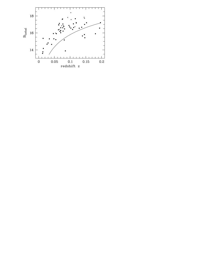
Figure 1: Hubble diagram for the sample. Circles mark the objects drawn from the HES, crosses the RX objects selected as ROSAT sources on HES plates. The solid line denotes the apparent magnitude of a QSO with $M_{B}=-23$ at the given redshift.

Table 1: Summary of observing campaigns.

Campaign	ID	Telescope	Instrument	CCD	Scale	# Obj.	Exposure
		ESO		ESO	[″/pix]		[seconds]
12/90	a	3.6 m	EFOSC1	#8	0.34	8	30
02/92	b	2.2 m	EFOSC2	#19	0.34	4	60
02/92	c	3.6 m	EFOSC1	#26	0.61	20	30
03/93	d	3.6 m	EFOSC1	#26	0.61	25	30

2.2 Observations

The data were obtained during several observing runs dedicated to low resolution slit spectroscopy with the principal aim to confirm the AGN nature of candidates (Reimers et al., 1996). During the early phase of the survey (between 1990 and 1993) the main instrument for this purpose was the ESO 3.6 m telescope with its focal reducer spectrograph EFOSC1. As a part of the acquisition procedure, taking at least one direct CCD image was mandatory; these images form the input dataset for the present analysis. To enable photometric comparison with our blue-sensitive photographic survey material, we always used a $B$ band filter. Typical exposure time was 30 s per image, under seeing conditions varying between $1\aas@@fstack{\prime\prime}1$ and $1\aas@@fstack{\prime\prime}7$. Some properties of the observational campaigns are listed in Table 1.

Although the imaging data were not initially meant to be used for host galaxy studies and the data are clearly low signal-to-noise, we found that extended ‘fuzz’ around pointlike nuclei could easily be detected already by eye in a good fraction of the low-redshift objects. Example images illustrating the typical data quality are displayed in Fig. 2, the full set of host galaxies is shown in Fig. 3. While detailed structural information generally cannot be extracted from these short exposure images, it turned out that estimation of integrated luminosities was indeed feasible.

Figure 2: Typical image quality for two redshifts. Top: HE 1043–1346 ($z=0.068$), bottom: HE 1110–1910 ($z=0.111$), all observed with EFOSC1 at the ESO 3.6m telescope. From left: image and contour including the nucleus, the same with the nucleus subtracted, radial profile (dashed line: QSO including nucleus, dotted line: PSF, points: residual galaxy, solid line: fits for disc and/or spheroid galaxy), curve of growth in apparent magnitudes. The lowest contour in each object is 25 and 26 mag arcsec^-2, respectively, with contour spacings of 0.5, and 1 mag arcsec^-2. Coordinates are given in arcsec.

Figure 3: The extracted host galaxies: Shown are the residual host galaxy images after subtraction of the scaled PSF star to remove the nuclear contribution. The size of the individual images is given in the last column of Table 3. (Continued next page)

Figure 4: continued

Observations of photometric standard star sequences during the same night were used to calibrate the instrumental magnitudes of point sources in the CCD images (cf. procedure described by Reimers et al., 1996). We did not perform corrections to the standard Bessell or Johnson systems, but since any such corrections should be below 0.1 mag for the type of objects discussed here, this aspect may be safely neglected. Large aperture measurements on the CCD frames gave the total (AGN + host) magnitudes. Together with the redshifts obtained from our low-resolution spectroscopy, we could place each source in a Hubble diagram as shown in Fig. 1.

It can be seen that the majority of our objects is located in the borderline region between high luminosity QSOs and lower luminosity Seyfert 1s. Since there seems to be a continuity of properties in all respects, we see no use in maintaining the historicaly grown arbitrary luminosity division and refer to all these objects as ‘QSOs’ henceforth.

3 Data analysis

3.1 Separation of stellar and nuclear light

To assess the galaxy apparent magnitudes, the nuclear and stellar light components needed to be separated. This was done by subtracting a scaled empirical two dimensional point-spread function (PSF) defined from a bright star in the object frame (cf. similar procedures employed e.g. by Véron-Cetty & Woltjer, 1990; Dunlop et al., 1993; McLeod & Rieke, 1994a, b; Rönnback et al., 1996; Scarpa et al., 2000; Sánchez & González-Serrano, 2003). Potential PSF stars had to be bright yet unsaturated, undistorted by cosmics, and spatially as close as possible to the QSO. The latter condition was particular important for a focal-reducer type instruments such as EFOSC where the shape of the PSF can vary significantly over the frame.

Prior to PSF subtraction, QSO and PSF star were recentered with respect to the pixel grid, so that their centroids coincided by better than 1/10th of a pixel. To avoid artificial broadening of either QSO or PSF star due to the necessary rebinning, both objects were shifted by equal amounts towards each other.

Following the definition of a PSF star, the factor of nuclear light to be subtracted had to be determined. An amount was subtracted as to yield a smooth, flat-top radial profile for the residual image, with no depression in the centre, a criterium sucessfully used by other authors (McLeod & Rieke, 1994a; Rönnback et al., 1996). For this calculation we utilised one-dimensional radial surface brightness profiles of the object and PSF star images, azimuthally averaged over elliptical isophotes.

Since the exact amount the nuclear contribution is a priori unknown, this procedure will usually lead to an underestimation of the galaxy flux, again by an unknown amount. However, two properties can be assumed valid for an arbitrary galaxy image: positive flux at all radii, and a surface brightness decreasing monotonously with radius. The former is always true; the latter is at least reasonable except for the – easily detectable – cases of strong spiral arms or circumnuclear starburst rings. The ‘monotony’ criterion will yield a higher flux for the residual galaxy than the ‘positive central flux’ criterion, and although it still leads to an oversubtraction of nuclear light (see next section), the amount of this oversubtraction will be minimised.

After subtraction of the AGN component, the residuals were always inspected to check for possible PSF mismatches. Typical mismatch patterns were ‘butterfly’ residuals with paired regions of positive and negative flux. In such cases it was first tried to apply slightly different centroiding displacements; in case of no improvement, a different star was used for the PSF. We finally succeeded to obtain reasonable PSF models for all objects in the sample.

The residual galaxy images, after subtraction of the nuclei, are shown in Fig. 3. The correction for oversubtraction discussed in the next section was not applied to these images.

3.2 Correction for oversubtraction

As the overestimation of nuclear light in the PSF subtraction process can result in a galaxy brightness too faint by several tenths of a magnitude (Abraham et al., 1992; Dunlop et al., 1993), we estimated the amount of oversubtraction from simulations. An array of artificial QSO+host images was created and treated with the methods described above. The image quality was chosen to match that of the actual data, and for each model several realisations of random photon shot noise were produced. Average correction terms and resulting uncertainties were calculated to give the amount of oversubtraction as well as the corresponding spread as a function of input model parameters.

The images were created as a function of redshift, galaxy morphological type, half-light radius, seeing, and nuclear and galaxy luminosity. For the morphological types two different models were assumed: An exponential disc model with

$$I(r)=I_{0}\exp\left[{-1.68\frac{r}{r_{0}}}\right]$$

for spiral and disc galaxies (Freeman, 1970), and a de Vaucouleurs’ model

$$I(r)=I_{0}\exp\left[{-7.67(\frac{r}{r_{0}})^{\frac{1}{4}}}\right]$$

for elliptical or bulge dominated galaxies (de Vaucouleurs, 1948). Here $I(r)$ is the radial surface brightness distribution in mag arcsec^-1, $I_{0}$ the central surface brightness and $r_{0}$ the radius in seconds of arc containing half of the total light. Because of the general difficulties in the analysis of galaxies with bright nuclei, a further breakdown in Hubble sub-types is usually not possible in ground-based data and was not attempted in these simulations.

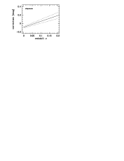
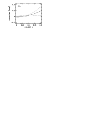
Figure 5: Correction terms for oversubtraction of the nuclear component as a function of redshift as determined in numerical simulations. The solid lines represent approximate averages over the range of adopted input parameters. The left panel shows the values for elliptical, the middle panel that for disc galaxies. The right panel is a combination of the two, to be used for hosts with unidentified galaxy type. Dotted lines bracket the range of values found in the simulations.

At each redshift, using two different half-light radii, galaxy-to-nuclear luminosity ratios, seeing values, as well as various photon shot noise realisations yielded a distribution of correction values. Figure 5 shows the resulting average correction terms – differences between ‘true’ and reconstruced magnitudes –, with suitable interpolation between the simulated redshifts. The range covered by the distributions is indicated by the dotted lines. As the distributions are considerably non-Gaussian, we have adopted the min–max range rather than rms scatter as uncertainty envelope.

The simulations show that the correction term depends mainly on the amount of angular extention, i.e. compactness, of the galaxy in comparison to the shape of the point like nucleus. In the case of relatively small seeing variations (full range $1\aas@@fstack{\prime\prime}4\pm 0\aas@@fstack{\prime\prime}3$) present in this data, the dominating parameters thus are the morphological type of the galaxy, ellipticals being more compact than discs, and the angular scale length, i.e. the combination of physical scalelength and redshift. Intrinsically more compact and more distant galaxies require larger corrections, thus also larger corrections for ellipticals than for disc galaxies for the same range of half-light radii. The effect from the range of scale lengths dominated over the effect of different seeing and the different ratios of nuclear and galaxy luminosities by a factor of two.

In the decomposition of quasar images, scale lengths are not a well constrained parameter, except for the case of very high S/N data (Abraham et al., 1992; Taylor et al., 1996) and it was also not possible to determine these numbers reliably for our sample. However, the half-light radii used in the simulations ($r_{0}=9$ kpc and 18 kpc for discs, 15 kpc and 30 kpc for ellipticals) are rather in the upper range of what is expected in the data. This leads to conservative estimates for the corrections: If an observed object has a host galaxy with a smaller scale length, its luminosity tends to be underestimated.

For many of our objects we could also not establish reliable morphological types (see below). To be able to deal with these cases we determined a correction term for hosts of unknown type by combination of the two type-specific relations, and this is shown in the right-hand panel of Fig. 5. The range of possible correction values is dominated by ellipticals for lower redshifts, and by discs at the high end. Note that the systematic differences between different models are negligible, considering the other error sources. This is an important feature of our adopted procedure, as it indicates that our PSF subtraction strategy allows us to estimate total host galaxy luminosities nearly independently of morphological type.

3.3 Host galaxy morphological types

The correction terms described above generally depend on galaxy type. If the type is known, the intrinsic uncertainty associated with the correction term is smaller than for the combined general correction relation shown in the middle panel of Fig. 5. It is therefore useful to determine galaxy types for as many objects as possible.

To determine individual galaxy types we fitted surface brightness distribution laws to the one-dimensional luminosity profiles of the nucleus-subtracted images, trying both the exponential disc and the de Vaucouleurs profiles as given above. The inner radius for the fit was fixed at one FWHM of the seeing, the outer radius was set at a S/N=1 in the galaxy profile.

To decide which model provided the better approximation, some authors (e.g. Rönnback et al., 1996; Taylor et al., 1996) compared the $\chi^{2}$ values of both model fits and adopted the model with the smaller $\chi^{2}$. This strategy is questionable, as the statistical significance of a decision is difficult to control, especially since real galaxies often fail to perfectly trace the theoretical distributions, but display spiral arms, knots, or other irregularities. More conservatively, we considered a galaxy type only to be safely determined if it could not be ruled out in a $\chi^{2}$ test at 95% confidence level, while at the same time the alternative model was rejected. Alltogether for 12 of the 57 objects in the sample we could establish galaxy types in this way – four discs and eight ellipticals. Further three objects not classified with the $\chi^{2}$ test were obviously spirals due to visible spiral arms.

3.4 Photometry

Galaxy magnitudes were measured by simulated aperture photometry in the PSF-subtracted residual images. Increasing the aperture radius in steps of one pixel yielded a curve-of-growth for the integrated flux with radius. Whenever the sky background was perfectly subtracted, these curves converged; non-convergence of the curve-of-growth, within the statistical uncertainties, indicated a nonperfect background subtraction. This yielded an excellent tool to optimise the background determination. The galaxy magnitude was adopted as the total integrated flux, after local background removal, to which the correction term for oversubtraction according to Fig. 5 was applied.

Pixels in the vicinity of the galaxies showing obvious artefacts of the CCD and cosmic ray events were eliminated from the analysis by creating a mask for each image. Masked pixels were not used, but effectively replaced by the average surface brightness value in the corresponding annulus. Likewise, projected neighbours such as foreground stars and background galaxies, but also physical companions were excluded (see discussion in Sect. 3.6 and Sect. 4.3 for a few exceptions).

3.5 Photometric uncertainties

We considered three major sources of uncertainties that contributed to the total error of the host galaxy magnitudes, apart from Poissonian errors in the individual images:

1. Uncertainties in the determination of the total flux from the curve-of-growth. The simulations show that in different shot noise realisations the derived flux fluctuates by $\pm 0.05$ mag (rms) out to $z=0.2$ for this image quality, independent of the galaxy type.

2. Errors in the correction for oversubtraction. According to Fig. 5, the range around the average is smaller than $\pm 0.1$ mag for $z<0.1$ and $\pm 0.15$ mag for $0.1<z<0.2$.

3. The uncertainty estimates for the corrections are only valid if the half-light radii of the objects in the sample are not much different from the values of $r_{0}$ adopted in the simulations. From the curve-of-growth analyses we estimate half-light radii between 9 and 18 kpc for most of the objects. As our data do not really have the angular resolution to probe into the central regions, it is likely that these values are somewhat too high for several of the objects. This unknown systematic error could push the luminosities of the most compact hosts to yet higher values. We have chosen to be conservative and to assume that the adopted corrections are, on average, correct.

The uncertainty estimates are summarised in Tab. 2, broken up into two redshift regions. For all but two objects, where photon shot noise dominates, these external errors determine the error budget.

Table 2: Photometric uncertainties for external error sources discussed in the text. The last column gives the combined uncertainty $\Delta B_{\mathrm{err,gal}}$ for two redshift ranges.

	Error source				$\Delta B_{\mathrm{err,gal}}$
$z$-range	(i)		(ii)		[mag]
$0.0\ldots 0.1$	$\pm 0$.	05	$\pm 0$.	1	$\pm 0$.	15
$0.1\ldots 0.2$	$\pm 0$.	05	$\pm 0$.	15	$\pm 0$.	2

3.6 Influence of companions, knots, tidal tails

Resolved or unresolved flux of companion objects, tidal tails or ‘knots’ of unknown nature in or around the host galaxies can contribute a significant amount of flux. This poses the question as to what constitutes ‘the host galaxy’? The answer is necessarily subjective, and depends on spatial and spectral resolution as well as S/N. An unspecific knot might be identified in high resolution, multicolour or spectroscopic data as a small companion galaxy in the process of being accreted, while this could not be inferred with lower resolution, single band imaging. Even then there is a gradual transition between a companion – which is not part of the host galaxy – and a clump within the host. Similar arguments can be brought forward in the case of tidal tails or bridges.

We took the approach to exclude the contribution of all visible compact asymmetries from the photometry of the host galaxies. Technically, as described in Sect. 3.4, we used the underlying smooth host galaxy contribution instead. We estimate that we exclude the contributions from all compact sources that would contribute more than 0.1 mag. Contributions from low surface brightness companions can not be ruled out, but even with higher S/N data these would be difficult to judge. For unresolved companions see also Sect. 4.3.

3.7 Systematic effects in host galaxy extraction

We now investigate whether our brightness estimation method could be biased by systematic effects that depend on the S/N of the data. Most crucial is our adopted strategy of determining the appropriate PSF scaling factor to subtract the nuclear component from the host galaxy. Two aspects are important in this context: (1) We have employed a criterion that, although it still should lead to an oversubtraction, is decidedly less conservative than the more frequently employed criterion of purely positive residuals. (2) Unlike several others, we have applied explicit corrections for oversubtraction determined from simulations.

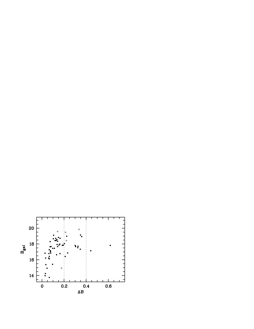
Figure 6: Difference $\Delta m$ in derived brightness of the host galaxies between the ‘monotony’ criterion for PSF subtraction used for analysis and the more conservative ‘positivity’ criterion for the surface brightness of the residual profile. Only for two objects is $\Delta m>0.4$. Open symbols mark the galaxies with higher uncertainties described above.

To test the level by which our ‘monotony’ criterion differs from the more conservative ‘positivity’ criteron, we have applied the latter to our dataset and compared the corresponding (uncorrected) aperture host magnitudes after PSF subtraction. The result of this exercise is shown in Fig. 6, where the difference $\Delta B$ between magnitudes determined with either method is plotted against apparent host magnitude. $\Delta B$ is smaller than 0.4 mag for all but two objects, and even smaller than 0.2 mag in over 70 % of the cases. Concerning the faintest objects, being the most difficult for separating host and nucleus, there is no systematic effect apparent from this relation that would systematically over- or underestimate these host galaxies in flux.

The correction for oversubtraction described in Sect. 3.2 and listed in Tab. 3 are $<0.25$ mag for all objects. As discussed in Sections 3.2 and 3.5, a possible systematic error in corrections could occur if some of the observed host galaxies were more compact than assumed in the simulations – but in that case the adopted corrections would be conservative again and the host luminosities rather under- than overestimated.

3.8 External test of PSF subtraction

The simulations described in secs. 3.2 and 3.5 demonstrate that our extracted host galaxy fluxes are quite reliable, and provide realistic error margins. In the light of the relatively low S/N of the data that this study is based on, we attempted to support this statement by taking into account a second, independent method and additional data.

In the course of a separate project with the aim to investigate the stellar composition of quasar host galaxies (Jahnke et al., 2003) we obtained multiband photometry for 19 objects out of the sample discussed here. New optical $V$, $R$ and $I$ band as well as near-infrared data were obtained. To separate the nuclear and host galaxy contributions for all of these images a new two-dimensional modelling algorithm was used (Kuhlbrodt et al., 2003).

Modelling the two-dimensional surface brightness distribution is usually superior to PSF scaling governed by radial profiles. However, in the case of low S/N data such a method becomes increasingly dominated by artefacts like PSF mismatch, asymmetries, and other deviations from the model assumptions when fitting a full parameter set (5–9 parameters). Thus without external constraints these methods can not be applied to the data presented here.

To reduce the number of free parameters and to guarantee a homogenenous treatment of all images of an object, the morphological parameters of a given object were determined globally for all bands. Using these parameters on the $B$ band images left only nuclear and host fluxes as free parameters. With these additional constraints modelling was successful for 12 of the 19 objects. In the remaining cases the size of the PSF mismatch or low S/N prevented the two-dimensional modelling to successfully converge.

Plotting the resulting apparent $B$ band host galaxy magnitudes derived in this independent way against the values derived from the PSF subtraction presented in this work yields the relation shown in Figure 7. Individual deviations up to 0.75 mag exist, but the values scatter symmetrically around the 1:1 correlation. The ensemble average difference is 0.00 mag ($\sigma=0.39$ mag).

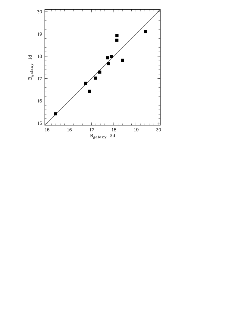
Figure 7: Apparent brightness of a 12 object ‘multicolour’ subsample for which two-dimensional modelling of the surface brightness distribution of the images was possible. Plotted is the ‘1d’ value of the host from this study against the ‘2d’ value. The solid line marks the 1:1 relation.

The 12 objects of the ‘multicolour’ subsample span both the full redshift and brightness range of the present sample (Fig. 8). The absence of any trend with apparent brightness suggests that the host galaxy fluxes are properly recovered and – for the upcoming discussion – that there is neither evidence that the luminosities of our objects are systematically overestimated, nor that any systematic effect is apparent to boost the host galaxies of the lower S/N.

4 Results

4.1 Apparent magnitudes

For 55 of the 57 objects in the sample, significant flux was detected in the PSF-subtracted image. In two cases the uncertainties are large and the residuals are dominated by shot noise, manifest also in significant fluctuations in the outer parts of the growth curves. Two further objects were observed near full moon and also these images are very noisy, although the host galaxies are clearly detected. In two further cases the PSF was poorly defined, so that the PSF subtraction must be considered quite uncertain. These six objects are marked by the ‘L’ flag in column 4 of Table 3 and by the open symbols in the relevant figures below. They will be treated separately in the subsequent discussion.

Redshift-dependent corrections for oversubtraction were applied using the relation shown in Fig. 5, type-specific in the case of the 15 objects with determined galaxy types, type-averaged values for the remaining ones. The individual values of the corrections $\Delta B_{\mathrm{gal}}$ are given together with the corrected apparent magnitudes $B_{\mathrm{gal}}$ and $B_{\mathrm{nuc}}$ in Table 3. Figure 8 shows the distribution of $B_{\mathrm{gal}}$ with redshift $z$. Error bars were derived from quadratic combination of internal Poissonian and external errors. For comparison we plotted the brightness of a field galaxy with Schechter luminosity ($M_{B}=-21.0$; Zucca et al., 1997) as a function of $z$.

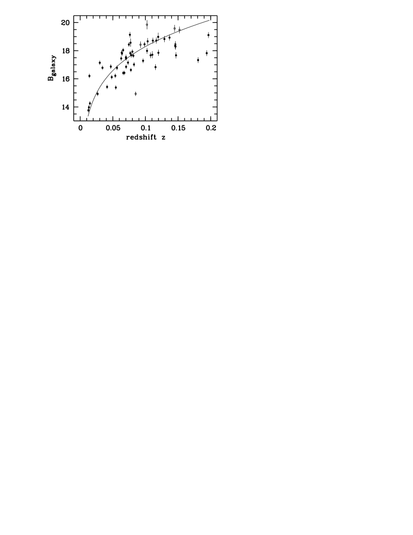
Figure 8: Distribution of the apparent galaxy magnitudes $B_{\mathrm{gal}}$ with redshift $z$ for the HES sample. Open symbols mark the objects with higher uncertainty. Errors are the quadractic combination of internal Poissonian and external errors. The solid line marks the apparent brightness of a galaxy with Schechter luminosity $L^{*}$ including galaxy $K$ correction for intermediate type (Sab) galaxy colours.

Table 3: The observed sample: Properties and results. The first two columns give object designations and redshifts, followed by a letter a–d indicating the observing campaign as listed in Table. Column ‘DQ’ lists ‘L’ if the data quality is considered to be low. Column ‘Type’ gives the morphological type when established (E: elliptical, D: disc, S: spiral arms visible). The next columns list the estimated correction for oversubtraction, the corrected apparent, and the inferred absolute magnitudes (standard $K$ correction). The next to last column lists the predicted $H$ band magnitude of the host galaxy, based on ‘normal’ galaxy colours. The last column gives the size of the object’s images in Fig. 3.

Object	$z$	C	DQ	Type	$\Delta\!B_{\mathrm{gal}}$		$B_{\mathrm{nuc}}$		$B_{\mathrm{gal}}$		$M_{B,\mathrm{nuc}}$		$M_{B,\mathrm{gal}}$		$M_{B,\mathrm{tot}}$		$M_{H,\mathrm{gal}}$		Image size [″]
HE 0317–2638	0.078	a			$-$0.	02	17.	45	16.	63	$-$20.	95	$-$22.	12	$-$22.	43	$-$25.	72	48
IR 03450+0055	0.030	a			$+$0.	05	14.	96	17.	14	$-$21.	89	$-$19.	87	$-$22.	05	$-$23.	47	48
HE 0348–2226	0.111	b			$-$0.	06	17.	95	17.	72	$-$21.	23	$-$21.	94	$-$22.	37	$-$25.	54	20
HE 0403–3719	0.056	b		D	$-$0.	02	16.	56	16.	78	$-$21.	11	$-$21.	16	$-$21.	88	$-$24.	46	38
HE 0414–2552	0.152	c	L		$-$0.	11	17.	34	19.	48	$-$22.	55	$-$21.	16	$-$22.	81	$-$24.	76	38
HE 0427–2701	0.064	a			0.	00	17.	60	17.	81	$-$20.	48	$-$20.	60	$-$21.	30	$-$24.	20	38
HE 0444–3449	0.181	a			$-$0.	15	16.	24	17.	33	$-$23.	93	$-$23.	68	$-$24.	53	$-$27.	28	38
HE 0444–3900	0.120	c			$-$0.	07	17.	45	18.	98	$-$21.	89	$-$20.	93	$-$22.	26	$-$24.	53	48
HE 0507–2710	0.146	c			$-$0.	11	17.	39	18.	30	$-$22.	38	$-$22.	15	$-$23.	00	$-$25.	75	48
HE 0517–3243	0.013	a			$+$0.	07	15.	69	13.	76	$-$18.	33	$-$20.	89	$-$21.	05	$-$24.	49	80
HE 0526–4148	0.076	c			$-$0.	01	17.	95	19.	14	$-$20.	50	$-$19.	70	$-$20.	92	$-$23.	30	38
HE 0529–3918	0.077	b			$-$0.	01	17.	35	18.	57	$-$21.	13	$-$20.	30	$-$21.	54	$-$23.	90	20
HE 0952–1552	0.108	d			$-$0.	06	16.	82	17.	67	$-$22.	55	$-$22.	21	$-$23.	13	$-$25.	81	48
IR 09595–0755	0.055	d			$+$0.	02	17.	27	15.	38	$-$20.	57	$-$22.	82	$-$22.	96	$-$26.	42	48
HE 1019–1414	0.077	a			$-$0.	01	17.	05	17.	82	$-$21.	73	$-$21.	33	$-$22.	30	$-$24.	93	38
PKS 1020–103	0.197	d			$-$0.	17	17.	41	19.	11	$-$23.	13	$-$22.	38	$-$23.	55	$-$25.	98	60
HE 1029–1401	0.085	a	L		$-$0.	03	14.	40	14.	94	$-$24.	60	$-$24.	48	$-$25.	28	$-$28.	08	48
HE 1043–1346	0.068	d		S	$-$0.	01	17.	99	16.	43	$-$20.	39	$-$22.	25	$-$22.	42	$-$25.	55	48
HE 1106–2321	0.081	d			$-$0.	02	15.	28	17.	64	$-$23.	49	$-$21.	54	$-$23.	66	$-$25.	14	48
HE 1110–1910	0.111	d		E	$-$0.	08	16.	81	18.	72	$-$22.	51	$-$21.	15	$-$22.	77	$-$25.	15	48
Q 1114–2846	0.070	c			$-$0.	01	16.	33	17.	54	$-$22.	13	$-$21.	28	$-$22.	54	$-$24.	88	48
PG 1149–1105	0.048	d			$+$0.	02	16.	00	16.	12	$-$21.	45	$-$21.	59	$-$22.	28	$-$25.	19	48
HE 1201–2409	0.137	d			$-$0.	09	16.	82	18.	93	$-$23.	16	$-$21.	71	$-$23.	40	$-$25.	31	38
HE 1213–1633	0.064	d			0.	00	17.	57	17.	86	$-$20.	55	$-$20.	59	$-$21.	32	$-$24.	19	38
HE 1217–1340	0.070	d		E	$-$0.	20	16.	73	17.	45	$-$21.	69	$-$21.	23	$-$22.	19	$-$25.	23	48
HE 1228–1637	0.102	d			$-$0.	05	16.	91	17.	99	$-$22.	23	$-$21.	64	$-$22.	71	$-$25.	24	48
HE 1235–0857	0.070	d		D	$-$0.	02	18.	37	16.	85	$-$19.	94	$-$21.	73	$-$21.	91	$-$25.	03	48
HE 1237–2252	0.096	d			$-$0.	04	18.	15	17.	29	$-$21.	18	$-$22.	45	$-$22.	72	$-$26.	05	48
HE 1239–2426	0.082	d			$-$0.	02	17.	48	17.	02	$-$21.	45	$-$22.	30	$-$22.	70	$-$25.	90	48
HE 1245–2709	0.066	d		E	$-$0.	20	17.	73	18.	04	$-$20.	83	$-$20.	72	$-$21.	46	$-$24.	72	48
HE 1248–1357	0.015	d		S	0.	00	17.	05	14.	25	$-$17.	97	$-$20.	85	$-$20.	92	$-$24.	15	70
IR 12495–1308	0.013	d			$+$0.	07	15.	65	13.	98	$-$18.	73	$-$20.	88	$-$21.	08	$-$24.	48	130
HE 1300–1325	0.047	a			$+$0.	03	16.	52	16.	87	$-$20.	95	$-$20.	85	$-$21.	66	$-$24.	45	38
HE 1309–2501	0.063	c		E	$-$0.	03	16.	87	17.	45	$-$21.	45	$-$21.	17	$-$22.	06	$-$25.	17	70
PG 1310–1051	0.034	d			$+$0.	04	15.	62	16.	79	$-$21.	13	$-$20.	15	$-$21.	51	$-$23.	75	48
HE 1315–1028	0.099	d		E	$-$0.	10	16.	95	18.	45	$-$22.	02	$-$20.	98	$-$22.	35	$-$24.	98	48
HE 1328–2509	0.027	d			$+$0.	05	16.	35	14.	93	$-$19.	80	$-$21.	58	$-$21.	81	$-$25.	18	48
HE 1335–0847	0.080	d		D	$-$0.	02	17.	23	17.	93	$-$21.	36	$-$21.	05	$-$21.	97	$-$24.	35	48
HE 1338–1423	0.041	c			$+$0.	03	15.	38	15.	42	$-$21.	96	$-$22.	15	$-$22.	82	$-$25.	75	90
HE 1348–1758	0.014	b			$+$0.	07	16.	02	16.	21	$-$19.	08	$-$19.	03	$-$19.	84	$-$22.	63	38
HE 1405–1545	0.194	d		D	$-$0.	24	16.	97	17.	83	$-$23.	78	$-$23.	79	$-$24.	49	$-$27.	09	38
PG 1416–1256	0.129	c			$-$0.	08	16.	70	18.	83	$-$23.	16	$-$21.	66	$-$23.	39	$-$25.	26	38
HE 1420–0903	0.117	d			$-$0.	07	18.	20	18.	72	$-$21.	37	$-$21.	38	$-$22.	11	$-$24.	98	38
HE 1434–1600	0.144	c		E	$-$0.	20	15.	58	17.	67	$-$24.	59	$-$23.	21	$-$24.	84	$-$27.	21	38
HE 1522–0955	0.146	d			$-$0.	11	15.	92	18.	34	$-$24.	33	$-$22.	61	$-$24.	52	$-$26.	21	38
RXJ 04407–3442	0.073	c			$-$0.	01	18.	39	17.	15	$-$19.	89	$-$21.	47	$-$21.	69	$-$25.	07	48
RXJ 04474–3309	0.078	c		E	$-$0.	01	17.	53	17.	68	$-$20.	87	$-$21.	11	$-$21.	74	$-$25.	11	38
RXJ 04485–3346	0.145	c	L		$-$0.	10	18.	09	19.	58	$-$21.	60	$-$20.	80	$-$22.	01	$-$24.	40	38
RXJ 05043–2554	0.120	c			$-$0.	07	17.	95	17.	85	$-$21.	44	$-$22.	06	$-$22.	52	$-$25.	66	48
RXJ 05079–3411	0.102	c	L		$-$0.	05	18.	71	19.	85	$-$20.	35	$-$19.	71	$-$20.	82	$-$23.	31	38
RXJ 10119–1635	0.066	d		E	$-$0.	20	18.	41	16.	41	$-$20.	05	$-$22.	37	$-$22.	49	$-$26.	37	48
RXJ 10596–1506	0.092	c	L		$-$0.	03	18.	75	18.	43	$-$20.	28	$-$21.	01	$-$21.	44	$-$24.	61	38
RXJ 11355–1328	0.075	c			$-$0.	01	18.	26	18.	44	$-$20.	18	$-$20.	36	$-$21.	02	$-$23.	96	48
RXJ 12167–3035	0.115	c		S	$-$0.	02	19.	38	16.	83	$-$20.	30	$-$23.	23	$-$23.	29	$-$26.	53	48
RXJ 12297–3153	0.054	c			$+$0.	02	17.	76	16.	22	$-$20.	06	$-$21.	94	$-$22.	13	$-$25.	54	48
RXJ 12570–1409	0.146	c	L		$-$0.	11	18.	48	18.	45	$-$21.	47	$-$22.	12	$-$22.	56	$-$25.	72	38
RXJ 13531–2802	0.103	c			$-$0.	05	18.	07	18.	66	$-$21.	13	$-$21.	03	$-$21.	82	$-$24.	63	38

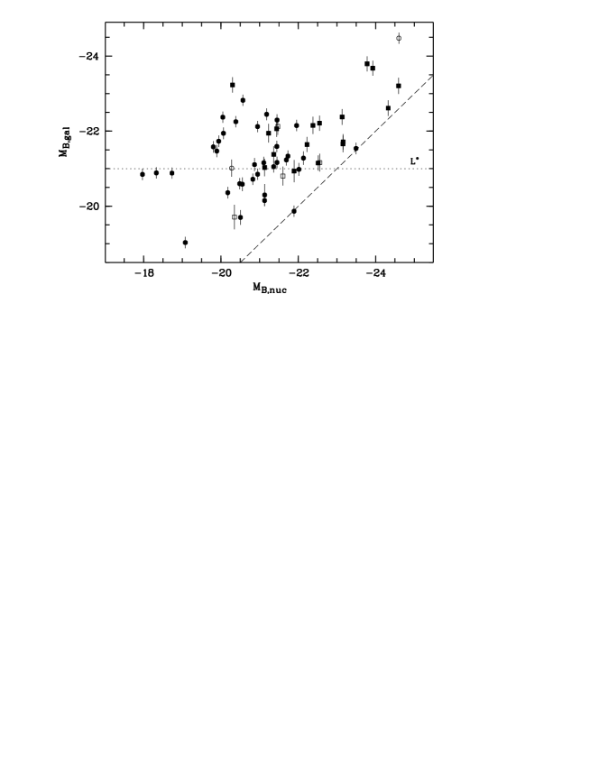
Figure 9: Host galaxy versus nuclear absolute magnitude in the $B$ band for all 57 objects in the sample. Redshift ranges are coded by different symbols, circles: $z<0.1$, squares: $0.1<z<0.2$. Open symbols denote the six objects with higher uncertainties marked in Table 3. The dashed line is a lower limit with slope 1.0, similar to the NIR relation of McLeod & Rieke, assuming the AGN to radiate with $L\sim 0.1L_{\mathrm{Edd}}$ (see text in Sect. 6). The horizontal dotted line marks the brightness of galaxies with Schechter luminosity $L^{*}$ for field galaxies.

4.2 Absolute magnitudes

To convert from apparent to absolute magnitudes we first corrected for Galactic foreground extinction, using the distribution of neutral hydrogen column density $N_{H}$ (Dickey & Lockman, 1990) and adopting $A_{B}=4.2\times N_{H}/58$ with $N_{H}$ given in units of $10^{20}\,\mathrm{cm}^{-2}$ (cf. Bohlin et al., 1978). The AGN $K$ correction was based on the usual formula

$$K_{\mathrm{nuc}}(z)=-2.5\,(\alpha+1)\,\log{(1+z)};$$

the value of the spectral index was taken as $\alpha=+0.45$. This is significantly different from the canonical value of $\alpha\approx-0.5$, but appropriate for the low-redshift range under discussion here (cf. the detailed discussion by Wisotzki, 2000b). Note that this $K(z)$ relation leads to slightly lower nuclear luminosities than usually obtained.

For the galaxies we adopted an approximate $K$ correction valid for inactive intermediate type (Sab) galaxies

$$K_{\mathrm{gal}}(z)=3.5\times z,$$

(Fukugita et al., 1995), valid for $z<0.3$. The $B$ band is particularly sensitive to $K$ correction effects as the difference between the Sab relation and the corresponding one for E galaxies is $\sim$0.35 mag at $z=0.2$. As the spectral energy distributions (SEDs) of our host galaxies is unknown, the $K$ correction adds a non-negligible additional uncertainty to the estimated absolute magnitudes of especially the objects near the upper redshift limit. Assuming a type-dependent $K$ correction for the 15 galaxies with established morphological types has little effects to our results, as these objects are all located at very low redshifts and have small corrections anyway.

Some previous studies (e.g., Smith et al., 1986; McLeod & Rieke, 1994a; Rönnback et al., 1996) have claimed host galaxy colours bluer than normal for their morphologically classified galaxy types. As will be discussed in Sect. 6.2, this might also be the case for our present sample. If that case the $K$ correction would be overestimated. If the SEDs were similar to intermediate to late-type spirals with ongoing star formation, the appropriate $K$ correction would be $K_{\mathrm{gal}}(z)\simeq 1.5\times z$, and a systematic error up to 0.4 mag (at $z=0.2$) could occur.

The estimated absolute magnitudes $M_{B,\mathrm{nuc}}$ and $M_{B,\mathrm{gal}}$ are also listed in Table 3. Figure 9 shows the properties of the sample in terms of nuclear and galaxy luminosities. The former range from $-18\ga M_{\mathrm{nuc}}\ga-24.5$ (mean $M_{\mathrm{nuc}}=-21.3$), the galaxy magnitudes range from $-19\ga M_{\mathrm{gal}}\ga-24$ (mean $M_{\mathrm{gal}}=-21.5$). When the low-quality objects are included, the mean value for the galaxy brightness remains unchanged, the mean nuclear luminosity increases by a marginal $0.1$ mag.

When dividing the sample into two subsets along the conventional though arbitrary division of Seyfert 1 and quasars at $M_{\mathrm{tot}}=-23$, a high-luminosity subsample of 11 objects and a low-luminosity subsample of 43 objects are formed. The average galaxy magnitude for the high-luminosity objects is $M_{\mathrm{gal}}=-22.6$, or about one magnitude brighter than for the whole sample (average nuclear luminosity is $M_{\mathrm{nuc}}=-23.1$). For the fainter subsample these values are $M_{\mathrm{gal}}=-21.2$ and $M_{\mathrm{nuc}}=-20.8$, respectively. Incorporating the low-quality objects leaves these values practically unchanged.

Three features in the distribution are worth noting:

1. The host galaxies are generally very bright. A large fraction of the objects, all in the case of the high-luminosity subsample, is brighter than an $L^{*}$ field galaxy, some by as much as a factor of $\sim$10.

2. There is a clear correlation between $M_{\mathrm{nuc}}$ and $M_{\mathrm{gal}}$, although this is dominated by the objects with the very brightest nuclei. No significant correlation is found for the low-luminosity subsample.

3. As expected from previous studies (e.g. McLeod & Rieke, 1995b), faint galaxies with bright nuclei are missing in the distribution. This is not a selection effect but solely due to a physical lower limit in host galaxy luminosity at given nuclear luminosity, since all of the host galaxies are detected.

4.3 Companions and morphological peculiarities

In nine of our images we identified possible close companion objects ($\leq 40$ kpc from the nucleus), and ongoing mergers in three further cases. Of course, we cannot dismiss the possibility that some of the ‘companions’ could be fore- or background objects. In general (unless noted otherwise) these objects have been masked out for the analysis of the host, excluding them from radial profile creation, model fitting, and luminosity estimation. Here we give some descriptive comments on the detected companions.

HE 0317–2638:

Two extra knots or companions in the host, $\sim$$6^{\prime\prime}$ ($\sim$14 kpc) from the center; included for brightness estimate of host, contribution is $\sim$30% of total luminosity.

HE 0517–3243

(= ESO 362-G18): Ongoing merging event, tidal arm with bright knot or companion galaxy.

IR 09595–0755:

Spectacular merging event, several knots and arcs. Object also known as MCG-01-26-011 or the ‘Sextans ring’.

HE 1110–1910:

Diffuse knot $\sim$$10^{\prime\prime}$ ($\sim$30 kpc) from centre is a spectroscopically confirmed companion (Wisotzki et al., in prep.). 25% of total luminosity, included in host brightness.

HE 1217–1340:

Image contains also a large edge-on spiral with no obvious interaction; probably a foreground galaxy. Two nearby objects ($\sim$$12^{\prime\prime}$ and $\sim$$15^{\prime\prime}$ distance, or $\sim$24 and $\sim$30 kpc, respectively) appear stellar. All excluded from flux integration.

HE 1228–1637:

Object at $\sim$$15^{\prime\prime}$ ($\sim$40 kpc), fainter by 0.5 mag, no tidal connection visible. Not included. This object happened to be observed during the spectroscopic follow-up; it is an emission-line galaxy at the QSO redshift.

HE 1239–2426:

Confirmed companion at $\sim$$12^{\prime\prime}$ ($\sim$27 kpc), included in luminosity estimate, 8% of total flux.

HE 1245–2709:

Faint object $\sim$$7^{\prime\prime}$ ($\sim$13 kpc) from host center, 6% of total flux. Included in total host brightness.

IR 12495–1308:

Active merger with several knots, tidal bridges and at least two pronounced nuclei. The second nucleus does not show any spectroscopic evidence for activity.

HE 1328–2509:

Knot well within the visible galaxy borders, $\sim$$12^{\prime\prime}$ ($\sim$9 kpc) from center, $<$5% of total flux (included). Could be a foreground star.

HE 1335–0847:

Object $\sim$$14^{\prime\prime}$ ($\sim$19 kpc) away from host, no visible tidal connection. 1.7 mag fainter than host galaxy, not included.

RXJ 13531–2802:

Two point like objects ($\sim$$12^{\prime\prime}$ and $\sim$$14^{\prime\prime}$ distance, or $\sim$$34$ and $\sim$$40$ kpc, respectively), brighter by 1.7 and 3 mag than the host galaxy, are most likely foreground stars.

Compared to high resolution imaging with HST (Disney et al., 1995; Fisher et al., 1996; Bahcall et al., 1997) we find that only a very small fraction of objects has close companions. We believe this to be in part an effect of data quality. Our data is less deep than the HST imaging and our images do not resolve faint companions closer than $\sim 2-3^{\prime\prime}$ to the nucleus. The close companion statistics by Bahcall et al. (1997) shows five out of their 20 luminous quasars to have close companions within $3^{\prime\prime}$ (projected to $z=0.2$). Of these only three contribute more than 0.1 mag to the total luminosity, none more than 0.25 mag, and and all but one of these quasars are radio-loud. An order-of-magnitude estimate from the single radio-quiet quasar yields a total of a few faint companions to be expected in the unresolved galaxy centers of the objects in our sample.

5 Comparison to existing studies

Although numerous imaging surveys of QSO host galaxies have been published, few of them provide sufficient sample size and cover a similar region of the Hubble diagram to be directly comparable to our sample. The list of comparison studies reduces to two when looking for the $B$ band. At other wavelengths the studies by McLeod & Rieke and Dunlop et al. are the most relevant for this sample.

5.1 B band studies

A larger $B$ band CCD study of host galaxies at low redshifts was published by Hutchings (1987) and Hutchings et al. (1989). A total of 50 objects were analysed in both $B$ and $R$, each half of which were radio-loud and radio-quiet QSOs, respectively. The RLQ and RQQ samples were selected to ‘match’ in their $z$ distributions. Only 11 RQQ and 8 RLQ hosts could be detected in the $B$ band.

There are no objects common to Hutchings’ and our sample so that only a statistical comparison is possible. The 11 detected RQQ host galaxies are on average $\sim$1 mag more luminous in $B$ than an inactive $L^{*}$ galaxy, similar to our results. However, the small sample size and its spread in luminosity and redshift space precludes a more detailed comparison.

More substantial is the study by Schade et al. (2000). They observed a sample of 76 low redshift ($z\leq 0.15$) AGN of low and intermediate luminosities ($-24<M_{B,\mathrm{tot}}<-18$) with the HST and ground based telescopes. The sample was X-ray selected from the Einstein Extended Medium Sensitivity Survey, thus not prone to selection effects from host galaxy morphology.

Ground based imaging was performed in the $B$ and $R$ bands. The 66 objects observed in the $B$ band show host galaxy properties similar to our lower-luminosity subsample, with a host galaxy luminosity range of $-23.0<M_{B,\mathrm{gal}}<-18.2$ and median of $-21.0$ (converted to Vega zeropoint from their AB magnitude system).

The authors report morphologies and colours not different from inactive galaxies. No strong merger events are observed, only central bars in a number of objects. Individual $B-I$ colours of their host galaxies show a large spread, which are, as the authors note, in part due to the separation of nucleus and host galaxy components. The mean colour $B-I\sim 2.2$ of their galaxy components is very similar to that of inactive galaxies without strong star formation.

Table 4: Optical and optical-NIR colours for ellipticals, Sbc, and Scd spirals, and intermediate types for galaxies with unidentified type (Fukugita et al., 1995; Fioc & Rocca-Volmerange, 1999).

Typ	$B\!-\!V$	$B\!-\!R$	$V\!-\!H$	$B\!-\!H$
E	0.96	1.57	3.05	4.0
interm.	0.77	1.33	2.85	3.6
Sbc	0.57	1.09	2.7	3.3
Scd	0.50	1.00	2.4	2.9

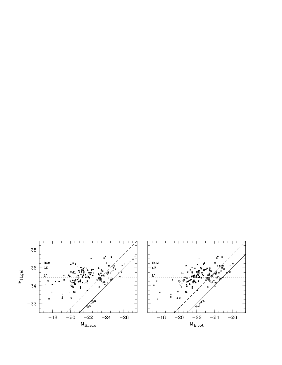
Figure 10: Predicted $H$ band galaxy magnitudes vs. the nuclear (left) and total (right) $B$ band magnitudes for the HES sample. Open symbols show the objects by McLeod & Rieke (1994a, b, 1995b). The horizontal lines are reference galaxy luminosities: Schechter $L^{*}$ of field galaxies, giant ellipticals (GE), and brightest cluster members. The solid diagonal line is the lower limit in galaxy $H$ band magnitude as a function of nuclear magnitude $M_{H,\mathrm{gal}}=M_{B,\mathrm{tot}}$ as first found by McLeod & Rieke, the dashed line is parallel to this relation but shifted by 1.5 mag to fit the HES sample.

5.2 NIR data by McLeod & Rieke

In three important papers, McLeod & Rieke studied the hosts of a total of $\sim$100 QSOs and Seyfert 1 galaxies in the near infrared $H$ band (McLeod & Rieke, 1994a, b, 1995b, hereafter MR1, MR2, MR3, or MR for the authors in general). Together with Schade et al. (2000) their studies are among the few where objects were selected in a well-defined way. Attempting to build representative samples, MR used subsamples from the Palomar-Green Bright Quasar Survey (Schmidt & Green, 1983) and the CfA Seyfert sample (Huchra & Burg, 1992).

The combined MR sample covers a somewhat larger range of nuclear absolute magnitudes than the HES, but the Hubble diagram occupancy of MR and HES samples is otherwise very similar. Unfortunately, there is only one object common to both studies (see sect. 5.4 below), so again the only way to compare the two sets of observations is by their statistical distribution of properties.

Instead of computing average statistical colours, we use our $B$ band measurements to predict $H$ band magnitudes for our sample assuming $B-H$ colours of normal inactive galaxies, depending on type if applicable. Typical optical to near infrared colours were taken from Fukugita et al. (1995) and Fioc & Rocca-Volmerange (1999) and are listed in Tab. 4.

For identified spirals and ellipticals we used $B-H=3.3$ and 4.0, respectively, for the remaining objects $B-H=3.6$ was adopted. The resulting predicted $H$ band luminosities are included in Tab. 3. Fig. 10 shows the distributions of observed MR and predicted HES $H$ band luminosities, plotted against nuclear absolute $B$ magnitude. However, a fair comparison between the HES and the MR samples is hampered by the fact that the ‘nuclear’ magnitudes quoted by MR are rather ill-defined: While for the Palomar-Green BQS these are basically isophotal, i.e. in good approximation total magnitudes, the Zwicky magnitudes given for the CfA sample contain highly unequal mixtures of light from stars in the central host galaxy regions and from the AGN. Being unable to reconstruct similar compound magnitudes for our objects, we have tried to bracket the correct distribution by plotting the HES data in two versions, shown in the two panels of Fig. 10: Total magnitudes (right-hand panel) are reasonable for the comparison between HES and BQS objects from MR1 and MR2; for the fainter AGN of the CfA sample galaxies (MR3), true nuclear magnitudes are more appropriate.

The figure displays distinct differences between observed and predicted $H$ band luminosities. In the MR data, several of the most luminous hosts are among the CfA galaxies, whereas in the HES sample the most luminous hosts also harbour very luminous nuclei. The distributions appear to be consistent in the low-luminosity Seyfert regime, but there is a strong mismatch at the high-luminosity end which is independent of the choice of nuclear magnitude (in fact, the mismatch increases when using ‘true nuclear’ magnitudes for the HES objects). Table 5 quantifies this in terms of average $M_{H,\mathrm{gal}}$ values for the two luminosity bins (MR restricted to $z\leq 0.2$, and using total magnitudes for the high-, true nuclear magnitudes for the low luminosities). While for the low-$L$ bin the samples are consistent within the expected uncertainties, the discrepancy for the high-luminosity QSOs is significant.

Table 5: Comparison of predicted $M_{H,\mathrm{gal}}$ as a function of total luminosity, compared with values measured by McLeod & Rieke. The McLeod & Rieke sample was restricted to $z\leq 0.2$ and the six ‘low quality’ objects have been removed from the HES sample. $N$ is the number of objects in each subsample, $\overline{z}$ is the average redshift, and $\Delta M$ is the difference in magnitudes between MR and HES hosts. Host galaxy colours of the HES objects were first assumed to be ‘normal’ (first set of columns), and then as similar to star-forming Scd galaxies (last columns; see text for details).

	MR								HES					normal				Scd-like
$M_{B}$	$N$	$\overline{z}$		$\overline{M}_{B}$		$\overline{M}_{H,\mathrm{gal}}$			$N$	$\overline{z}$		$\overline{M}_{B}$		$\overline{M}_{H,\mathrm{gal}}$		$\Delta M$		$\overline{M}_{H,\mathrm{gal}}$		$\Delta M_{\mathrm{Scd}}$
$M_{B,\mathrm{tot}}\leq-23$	43	0.	13	$-$24.	0	$-$25.	1		11	0.	14	$-$23.	8	$-$26.	1	1.	0	$-$25.	3	0.	2
$-23<M_{B,\mathrm{tot}}$	46	0.	019	$-$20.	5	$-$24.	7		43	0.	07	$-$20.	8	$-$24.	8	0.	1	$-$24.	0	$-$0.	7

Before discussing for possible explanations, we identify one technical point, often overlooked, that might reduce the discrepancy but cannot account for the effect as such. The decomposition into nuclei and hosts allowed us to apply appropriate $K$ corrections to both components separately. Within the MR sample this was not possible, as the contributions of galaxy light to the total $B$ magnitudes were not known. Applying a QSO-type $K$ correction to such a composite $B$ magnitude, as done by MR, leads invariably to an overestimation of the object’s luminosity; the effect will be small when the nucleus outshines the host, and largest for a low-luminosity nucleus in a bright host at relatively high redshift. Using our own data we have estimated that this effect could result in a bias of $M_{B,\mathrm{tot}}\sim 0.5$ mag for extreme cases, however it will generally be much smaller.

We note in passing that in preparing the comparison in Fig. 10 and Tab. 5, we adopted the same QSO $K$ correction as MR, thus using $\alpha=-0.5$ rather than the more previously used value of $\alpha=+0.45$.

5.3 Studies by Dunlop et al.

Dunlop et al. (1993), Taylor et al. (1996), McLure et al. (1999), Hughes et al. (2000), Nolan et al. (2001) and Dunlop et al. (2003) compared the properties of RLQs and RQQs at low redshifts. From the catalogue of Véron-Cetty & Véron (1991) they selected samples of $\sim$10 objects for each class with $z\leq 0.35$ and $M_{V,\mathrm{tot}}\leq-23$, to ‘match’ in $z$ and $V$ distribution, and obtained HST F675W ($\sim$$R$) band and ground based $K$ band imaging as well as off-nuclear host galaxy spectra. Due to the selection the sample has a smaller Hubble diagram coverage than our sample.

From morphological analysis all except two RQQ host galaxies were found to be large ellipticals. Both the derived $R-K$ colours and the spectra showed SEDs consistent with the morphological classification, i.e. a dominant evolved, red stellar population with no enhanced blue component. They determined average values of $M_{K,\mathrm{gal}}=-26.3$ and $M_{R,\mathrm{gal}}=-23.5$ for their combined RQQ and RLQ samples, the host galaxies of the RLQ being more luminous than their RQQ counterparts by about 0.5 mag.

Their samples were primarily selected for the comparison of the properties of the host galaxies of RQQs, RLQs and radio galaxies and are not statistically complete or representative. We still want to use their RQQ sample for comparison because of the high luminosity and the reliable methods applied in extracting the host galaxy properties.

Our bright subsample has a very similar total luminosity, $M_{V,\mathrm{tot}}=-23.8$ when assuming $M_{V}\simeq M_{B}$, compared to $M_{V,\mathrm{tot}}=-24.0$ for the Dunlop RQQ sample. Their RQQ host galaxies have an $R$ band luminosity of $M_{R,\mathrm{gal}}=-23.3$. Converting again our average $B$ host luminosity from Sect. 4.2 above to the $R$ band, assuming $B-R=1.3$, valid for intermediate type inactive galaxies (Fukugita et al., 1995, see Tab. 4), we arive at a predicted $M_{R,\mathrm{gal}}=-24.3$, much brighter than actually observed for their sample.

5.4 Comparison of individual objects

The HES sample contains only two objects that were already studied by others, in various photometric bands. We derive colours from the measured apparent magnitudes and compare them to those of intermediate type (Sab) inactive galaxies, including the $K$ corrections for both colours taken from Coleman et al. (1980), Fukugita et al. (1995), and Yoshii & Takahara (1988).

PKS 1020–103,

is an intermediately luminous RLQ at $z=0.197$. It is one of the objects that we also analysed with two-dimensional modelling, which in this case yielded a luminosity less than 0.1 mag different. The object was observed by Dunlop et al. (2003) in the $R$ band. The resulting $B-R=2.0$ is identical to the corresponding value expected for a normal galaxy at this redshift. Thus this object shows no unusual colours, which is confirmed by Dunlop et al. and Nolan et al.

PG 1416–1256,

$z=0.129$, has been observed by McLeod & Rieke (1994b) in the $H$ band, yielding $B-H=3.45$ whereas a normal galaxy at this redshift on average shows $B-H=4.2$.

Thus one of these two objects appears much bluer than comparable inactive early type spirals.

6 Discussion

In Sections 3.5 through 3.8 we evaluated possible sources for systematic biases in extracted host galaxy luminosities, and concluded that we accounted for all major systematic effects. As previously found, there exists a lower limit in host galaxy luminosity as a function of nuclear luminosity.

As the main result of this analysis we find that high luminosity QSOs are hosted by extraordinarily luminous (in the $B$ band) galaxies. When comparing our data with other samples observed at longer wavelengths, there is a significant discrepancy when assuming host galaxy colours typical for inactive galaxies. We see two options to resolve this discrepancy: Either our sample contains more luminous galaxies than those of previous studies, possibly due to QSO sample selection biases. Alternatively, the phenomenon could be explained by unusually blue host galaxy colours. We now investigate each of these options in more detail.

6.1 Are previous samples biased?

If the HES selection procedure of low-redshift QSOs is largely unbiased with respect to host galaxy properties, could then the apparent excess of high-luminosity hosts be related to an incompleteness of previous samples? Unfortunately there is very little overlap between the sky coverage of the HES and other surveys, so the direct route to test this on an object-to-object comparison is not possible.

As already mentioned in the introduction, most optical QSO surveys discriminate against objects with non-stellar morphology and are thereby biased in a straightforward way. The amount of incompleteness introduced into the samples depends on several factors: limiting surface brightness of the survey imaging data (often photographic plates); photometric band employed; definition of ‘extendedness’. For the Palomar-Green survey (Schmidt & Green, 1983), probably the most important supplier of luminous low-$z$ QSOs and the principle source for MR, Köhler et al. (1997) estimated an incompleteness of up to a factor of $\sim 3$–5 based on a comparison of measured number counts in the HES. However, in a more recent study with the full HES, Wisotzki et al. (2000) showed an incompleteness of only $\sim$1.5. It is not clear if this incompleteness is brightness dependent but it is likely that high luminosity QSOs suffer less than objects at the detection limit. Overall, we can not completely rule out that the PG incompleteness might have an effect, but probably the influence of any possible selection bias would be small.

For the lower luminosity CfA Seyfert sample investigated by MR, which is based on a dedicated galaxy catalogue, no selection bias against extended objects is expected. Correspondingly, the $B-H$ host galaxy colours in combination with the HES are very consistent with ‘inactive’ colours for the low-luminosity Seyferts.

6.2 Blue colours due to younger population age?

After excluding selection biases as a dominant factor, we are left with the implication that we see bluer than normal colours for some of our host galaxies. In particular, there seems to be a division in host galaxy colours that is correlated with luminosity. The low luminosity QSO sample seems to show ‘normal’ colours for the hosts and a wide range of nuclear luminosities. These objects seem to be normal galaxies in many aspects except for the active nuclei in their centers.

The higher luminosity QSOs seem to be bluer than normal in optical–NIR colours by $\sim$1 mag. Even though the number of objects involved is small (eleven objects), the difference is not dominated by e.g. the most luminous hosts in the sample. This unusual colour has two effects: (1) The $(B-H)$ colour would numerically decrease, and (2) the $K$ correction for the galaxy would become smaller. Both effects operate in the same direction, making the predicted $H$ band magnitudes fainter. The first effect causes a constant offset for all objects, the second is redshift-dependent and largest for the high-luminosity objects at $z\sim 0.2$.

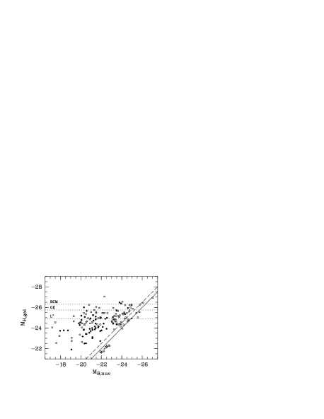
Figure 11: Predicted HES and observed MR $H$ band luminosities, computed with Scd-type colours and $K$ corrections. Symbols and lines as in Fig. 10.

To illustrate the consequences, we used the Scd-type colours listed in Tab. 4, together with appropriate $K$ corrections from Griersmith et al. (1982) and Fukugita et al. (1995), and recalculated the predicted $H$ band magnitudes. The resulting colours of $(B-H)\sim 2.9$ and a $B$ band $K$ correction of $1.5\times z$ would result in an $H$ band ‘dimming’ of the brightest HES galaxies by $\sim$1 mag. Note that such colours would be also bring the $B$ luminosity of PG 1416–1256 from Sect. 5.4 into agreement with the results from MR. Fig. 11 shows the changes in the comparison of MR and HES samples when an Scd-like stellar population is assumed. The strongest changes occur at relatively high $z$, affecting the most luminous objects. The discrepancy between the bright end of the samples is largely removed. Colours of $(B-H)\sim 2.5$ are however more typical of late type spirals. Such morphological types would be contrary to the established fact that luminous AGN reside predominantly in early type galaxies.

Conversely, if our luminous hosts are indeed mostly of early galaxy type, such blue colour would be somewhat unexpected. Possible explanations could be ongoing star formation at a rate substantially higher than expected, an overall younger stellar population, or a recent starburst.

The resulting composite spectral energy distributions would at short wavelengths be dominated by the youngest stars, but the bulk of radiation in the red would come from the old stellar population. Note that virtually all of the bright HES objects are at the high redshift end of our sample, $z\ga 0.1$. For these objects we start to measure in the rest-frame $U$ band rather than in $B$. Because of the strong 4000 Å break displayed by old stellar populations, already a relatively small fraction of very young stars could account for a significant rest-frame $U$ band excess, boosting our measured $B$ band magnitudes, but show relatively little effect in the other colours.

To give an order-of-magnitude estimate, we compute the effect of a simple instantaneous burst population of young stars and the masses nessessary to produce these blue colours. Adopting the simple two-component model of an old and a young stellar population, we used the colours and luminosities for starburst models given by Leitherer & Heckman (1995). The inferred mass of a burst population depends mainly on the the assumed burst age, yielding values of $\sim$1% for an age of $10^{6.5}$ yrs and $\sim$5% for an age of $10^{7}$ yrs. For a $10^{8}$ yrs population already a significant fraction is required.

Are such blue colours compatible with previous results? Some earlier studies have indicated bluer than normal colours for host galaxies, however others find largely normal values:

• The abovementioned study by Hutchings et al. (1989) finds $B-R=0.94$ for their RQQ hosts and even $B-R=0.29$ for the RLQ hosts, compared to $B-R=1.4$ for inactive Sab spirals and $B-R=1.6$ for inactive ellipticals.

• Rönnback et al. (1996) and Örndahl & Rönnback (2001) obtain rest frame $B-V$ colours for three elliptical RQQ host galaxies, bluer than normal by 0.6 mag. These object have similar luminosities than our luminous objects.

• The early spectrocopic studies by Boroson & Oke (1984) and Boroson et al. (1985) resulted in a range of colours, down to $B-V\simeq 0.2$, the colour of very late spirals. Five of six QSOs with $B-V<0.5$ resided in luminous early type galaxies (Stockton & Ridgway, 1991; Hutchings & Neff, 1992; Bahcall et al., 1997; Márquez et al., 2001), all of these RLQs.

• A reanalysis of HST data of nine host galaxies by McLeod & Rieke (1995a) shows a tendency for blue colours in $V-H$, an excess by $\sim$0.5 mag compared to inactive Sab galaxies or $\sim$0.7 mag to ellipticals.

So several studies find evidence for bluer colours. On the other hand, as noted above, the more luminous sample investigated by Dunlop et al. (2003) and Nolan et al. (2001), all elliptical galaxies by morphology, was found to show $R-K$ colours and spectra typical of old evolved stellar populations, with ages $\ga 8$ Gyrs and no traces of star formation. Similarly, normal colours have been reported for the (lower-luminosity) X-ray selected objects by Schade et al. (2000) and for the multicolour study of low-luminosity (mostly spiral) Seyfert galaxies by Kotilainen & Ward (1994). This agrees well with the results our low luminosity subsample. Furthermore it should be expected that the most luminous elliptical galaxies, with low remaining gas content, also show old stellar populations and colours. If Dunlop et al. find only such objects, then this may or may not be an effect of sample selection. On the other hand, at least in the luminosity regime of our sample, there exists a range of host galaxies colours, from normal to very blue.

Due to the current lack of detailed diagnostics, we prefer to refrain from speculating on the cause for the enhanced blue colours at this point. Obvious candidates are tidal interaction, or minor or major mergers. If all or some nuclear activity is triggered by such events then it is well possible that also star formation is induced in the host galaxy by the same process. However our very limited data quality does not allow a meaningful correlation of colour and either companion statistics or a measurement of distortion as an indicator for interaction. Deep higher resolution data and in particularly a well defined comparison sample of inactive galaxies are required for this task.

7 Conclusions

We analysed a new sample of low-$z$ AGN, encompassing both luminous QSOs and intermediate-luminosity Seyfert galaxies. The objects were selected from the Hamburg/ESO survey, for which host galaxy dependent selection biases are greatly reduced compared to other optical surveys.

We found that the host galaxies in our sample are generally very luminous, typically around $L^{\star}$ for the lower nuclear luminosities, and several times brighter for high luminosity QSOs. From a statistical comparison to studies in other bands we conclude that the latter show signs of significantly bluer colours ($B-H\sim 2.5$) than inactive galaxies. We argue that the mismatch of observed and predicted $H$ band magnitudes for the most luminous QSOs in the Palomar-Green and HES samples is not likely to be explained by selection effects.

These discrepancies can be resolved when invoking an additional contribution from younger stars, adding blue light to the bulk emission of an old(er) evolved stellar population. In case of a recent starburst the inferred stellar masses would only need to comprise a few percent of the total luminous mass. Such a starburst could be induced e.g. by a minor or major merging event that at the same time is triggering the nuclear activity in luminous QSOs.

More and different data is required to test the distribution and origin of bluer colours. As one option multiband imaging would allow homogenous photometry and direct measurement of colours. To identify the source of an enhanced star formation rate, spectroscopy is required. Only with spectra, timescales and masses of the star forming processes become available. In fact, very little data involving either direct multiband photometry or QSO host spectroscopy can be found in the literature. Most of the few existing investigations reported host galaxy colours that are bluer than those of normal galaxies, consistent with our inferences.

References

- Abraham et al. (1992) Abraham R. G., Crawford C. S., McHardy I. M., 1992, ApJ, 401, 474
- Bade et al. (1995) Bade N., Fink H. H., Engels D., Voges W., Hagen H.-J., Wisotzki L., Reimers D., 1995, A&AS, 110, 468
- Bahcall et al. (1997) Bahcall J. N., Kirhakos S., Saxe D. H., Schneider D. P., 1997, ApJ, 479, 642
- Bohlin et al. (1978) Bohlin R. C., Savage B. D., Drake J. F., 1978, ApJ, 224, 132
- Boroson & Oke (1984) Boroson T. A., Oke J. B., 1984, ApJ, 281, 535
- Boroson et al. (1985) Boroson T. A., Persson S. E., Oke J. B., 1985, ApJ, 293, 120
- Canalizo & Stockton (2000) Canalizo G., Stockton A., 2000, ApJ, 528, 201
- Coleman et al. (1980) Coleman G. D., Wu C.-C., Weedman D. W., 1980, ApJS, 43, 393
- de Vaucouleurs (1948) de Vaucouleurs G., 1948, Ann. Astrophys., 11, 247
- Dickey & Lockman (1990) Dickey J. M., Lockman F. J., 1990, ARAA, 28, 215
- Disney et al. (1995) Disney M. J., Boyce P. J., Blades J. C., Boksenberg A., Crane P., Deharveng J. M., Macchetto F., Mackay C. D., Sparks W. B., Phillipps S., 1995, Nature, 376, 150
- Dunlop et al. (2003) Dunlop J. S., McLure R. J., Kukula M. J., Baum S. A., O’Dea C. P., Hughes D. H., 2003, MNRAS, 340, 1095
- Dunlop et al. (1993) Dunlop J. S., Taylor G. L., Hughes D. H., Robson E. I., 1993, MNRAS, 264, 455
- Ferrarese & Merrit (2000) Ferrarese L., Merrit D., 2000, ApJ, 539, L9
- Fioc & Rocca-Volmerange (1999) Fioc M., Rocca-Volmerange B., 1999, A&A, 351, 869
- Fisher et al. (1996) Fisher K. B., Bahcall J. N., Kirhakos S., Schneider D. P., 1996, ApJ, 468, 469
- Freeman (1970) Freeman K. C., 1970, ApJ, 160, 812
- Fukugita et al. (1995) Fukugita M., Shimasaku K., Ichikawa T., 1995, PASP, 107, 945
- Gebhardt et al. (2000) Gebhardt K., Bender R., Bower G., Dressler A., Faber S. M., Filippenko A. V., Green R., Grillmair C., Ho L. C., Kormendy J., Lauer T. R., Magorrian J., Pinkney J., Richstone D., Tremaine S., 2000, ApJ, 539, L13
- Griersmith et al. (1982) Griersmith D., Hyland A. R., Jones T. J., 1982, AJ, 87, 1106
- Hernquist (1989) Hernquist L., 1989, Nature, 393, 90
- Huchra & Burg (1992) Huchra J., Burg R., 1992, ApJ, 393, 90
- Hughes et al. (2000) Hughes D. H., Kukula M. J., Dunlop J. S., Boroson T., 2000, MNRAS, 316, 204
- Hutchings (1987) Hutchings J. B., 1987, ApJ, 320, 122
- Hutchings et al. (1989) Hutchings J. B., Janson T., Neff S. G., 1989, ApJ, 342, 660
- Hutchings & Neff (1992) Hutchings J. B., Neff S. G., 1992, AJ, 104, 1
- Jahnke et al. (2003) Jahnke K., Kuhlbrodt B., Wisotzki L., 2003, MNRAS, in prep.
- Kauffmann & Haehnelt (2000) Kauffmann G., Haehnelt M., 2000, MNRAS, 311, 576
- Köhler et al. (1997) Köhler T., Groote D., Reimers D., Wisotzki L., 1997, A&A, 325, 502
- Kotilainen & Ward (1994) Kotilainen J. K., Ward M. J., 1994, MNRAS, 266, 953
- Kuhlbrodt et al. (2003) Kuhlbrodt B., Wisotzki L., Jahnke K., 2003, submitted to MNRAS
- Leitherer & Heckman (1995) Leitherer C., Heckman T. M., 1995, ApJS, 96, 9
- McLeod & Rieke (1994a) McLeod K. K., Rieke G. H., 1994a, ApJ, 420, 58
- McLeod & Rieke (1994b) McLeod K. K., Rieke G. H., 1994b, ApJ, 431, 137
- McLeod & Rieke (1995a) McLeod K. K., Rieke G. H., 1995a, ApJ, 454, L77
- McLeod & Rieke (1995b) McLeod K. K., Rieke G. H., 1995b, ApJ, 441, 96
- McLure & Dunlop (2002) McLure R. J., Dunlop J. S., 2002, MNRAS, 331, 795
- McLure et al. (1999) McLure R. J., Kukula M. J., Dunlop J. S., Baum S. A., O’Dea C. P., Hughes D. H., 1999, MNRAS, 308, 377
- Magorrian et al. (1998) Magorrian J., Tremaine S., Richstone D., Bender R., Bower G., Dressler A., Faber S. M., Gebhardt K., Green R., Grillmair C., Kormendy J., Lauer T., 1998, AJ, 115, 2285
- Márquez et al. (2001) Márquez I., Petitjean P., Théodore B., Bremer M., Monnet G., Beuzit J.-L., 2001, A&A, 371, 97
- Nolan et al. (2001) Nolan L. A., Dunlop J. S., Kukula M. J., Hughes D. H., Boroson T., Jimenez R., 2001, MNRAS, 323, 308
- Örndahl & Rönnback (2001) Örndahl E., Rönnback J., 2001, in Marqués I., Masegosa J., del Olmo A., Lara L., García E., Molina J., eds, QSO Hosts and their Environments, Kluver Academic/Plenum Publishers, p. 61
- Reimers et al. (1996) Reimers D., Köhler T., Wisotzki L., 1996, A&AS, 115, 235
- Rönnback et al. (1996) Rönnback J., Van Groningen E., Wanders I., Örndahl E., 1996, MNRAS, 283, 282
- Sánchez & González-Serrano (2003) Sánchez S. F., González-Serrano J. I., 2003, A&A, accepted
- Scarpa et al. (2000) Scarpa R., Urry C. M., Falomo R., Pesce J. E., Treves A., 2000, ApJ, 532, 740
- Schade et al. (2000) Schade D., Boyle B. J., Letawsky M., 2000, MNRAS, 315, 498
- Schmidt & Green (1983) Schmidt M., Green R. F., 1983, ApJ, 269, 352
- Smith et al. (1986) Smith E. P., Heckman T. M., Bothun G. D., Romanishin W., Balick B., 1986, ApJ, 306, 64
- Stockton (1982) Stockton A., 1982, ApJ, 257, 33
- Stockton & Ridgway (1991) Stockton A., Ridgway S. E., 1991, AJ, 102, 488
- Taylor et al. (1996) Taylor G. L., Dunlop J. S., Hughes D. H., Robson E. I., 1996, MNRAS, 283, 930
- Véron-Cetty & Véron (1991) Véron-Cetty M.-P., Véron P., 1991, A Catalogue of Quasars and Active Nuclei, 5th Edition. ESO Scientific Report #10
- Véron-Cetty & Woltjer (1990) Véron-Cetty M.-P., Woltjer L. J., 1990, A&A, 206, 69
- Wisotzki (2000a) Wisotzki L., 2000a, A&A, 353, 853
- Wisotzki (2000b) Wisotzki L., 2000b, A&A, 353, 861
- Wisotzki et al. (2000) Wisotzki L., Christlieb N., Bade N., Beckmann V., Köhler T., Vanelle C., Reimers D., 2000, A&A, 358, 77
- Wisotzki et al. (1996) Wisotzki L., Köhler T., Groote D., Reimers D., 1996, A&AS, 115, 227
- Yoshii & Takahara (1988) Yoshii Y., Takahara F., 1988, ApJ, 326, 1
- Zucca et al. (1997) Zucca E., Zamorani G., Vettolani G., Cappi A., Merighi R., Mignoli M., Stirpe G. M., MacGillivray H., Collins C., Balkowski C., Cayatte V., Maurogordato S., Proust D., Chincarini G., Guzzo L., Maccagni D., Scaramella R., Blanchard A., Ramella M., 1997, A&A, 326, 477