Non-commutative inflation and the CMB
Abstract
Non-commutative inflation is a modification of standard general relativity inflation which takes into account some effects of the space-time uncertainty principle motivated by ideas from string theory. The corrections to the primordial power spectrum which arise in a model of power-law inflation lead to a suppression of power on large scales, and produce a spectral index that is blue on large scales and red on small scales. This suppression and running of the spectral index are not imposed ad hoc, but arise from an early-Universe stringy phenomenology. We show that it can account for some loss of power on the largest scales that may be indicated by recent WMAP data. Cosmic microwave background anisotropies carry a signature of these very early Universe corrections, and can be used to place constraints on the parameters appearing in the non-commutative model. Applying a likelihood analysis to the WMAP data, we find the best-fit value for the critical wavenumber (which involves the string scale) and for the exponent (which determines the power-law inflationary expansion). The best-fit value corresponds to a string length of .
pacs:
pacs: 98.80.CqI Introduction
General relativity will break down at very high energies in the early Universe when quantum effects are expected to become important. If the very early Universe is described by a period of inflation Guth , as in the current paradigm of cosmology, and if the period of inflation lasts sufficiently long (as it does in most current scalar field-driven inflationary models), then, since the wavelength of perturbations which are observed today emerged from the Planck region in the early stages of inflation, in principle the quantum theory of gravity should leave an imprint on the primordial spectrum of perturbations (see initial for the first discussion of this effect; see review for a recent review containing a comprehensive list of references, and recent for some of the latest papers on this issue). The nature of these imprints will remain an open question as long as we lack a complete theory of quantum gravity. If we assume that string theory is a promising framework for quantum gravity, it is of interest to explore specific stringy corrections to the spectrum of fluctuations.
The standard concordance CDM model, which can arise from an inflationary background cosmology in which the quasi-exponential expansion of space is driven by a scalar field, provides a good fit to the recent WMAP Spergel:2003cb ; Kogut:2003et ; Verde:2003ey ; Peiris:2003ff and earlier observations. This implies, in particular, that any stringy corrections to general relativity will be constrained by the properties of the observed cosmic microwave background (CMB) anisotropies. Although there is no signature in CMB data of statistically significant deviations from the predictions of the standard paradigm, the unexpectedly low quadrupole and octopole Spergel:2003cb are intriguing, in particular since a similar deficit of power on these large angular scales was also seen in the earlier COBE maps. Thus, although the lack of power on the largest scales may simply be a statistical effect (and different approaches to statistical analysis yield differing results concerning the statistical significance of the lack of power ge ), early Universe explanations of this lack of power are not ruled out and are worth exploring, provided that the explanations are not ad hoc.
Recent papers low1 ; low2 ; Contaldi ; Cline ; Feng have attempted to explain the low quadrupole and octopole, typically via a finely-tuned inflationary potential or an ad hoc cut-off in the spectrum (see Ref. Yokoyama for the earlier work about this suppression). In Ref. KYY , supergravity inflation is shown to lead to a possible running of the power spectrum which tends to be blue on large scales. In Ref. bfm , some corrections to general relativity inflation motivated by brane-world scenarios (correction terms in the Friedmann equations and velocity-dependent potentials) were studied, and it was shown that they may account for the suppression of power. Here, we investigate consequences of a more basic stringy effect, namely the space-time uncertainty relation uncpr
| (1) |
where are the physical space-time coordinates and is the string scale. In Alexander:2001dr , it was shown that this principle may yield inflation from pure radiation. A more modest approach was pioneered in Brandenberger:2002nq , where the consequences were studied of imposing Eq. (1) on the action for cosmological perturbations on an inflationary background (generated in the usual way).
Space-time non-commutativity excep at high energies in the early Universe leads to a coupling between the fluctuations generated in inflation and the background Friedmann model that is nonlocal in time. In addition, the uncertainty relation is saturated for a particular comoving wavelength when the corresponding physical wavelength is equal to the string length. Thus, fluctuation modes must be considered to emerge at this time (a time denoted by later in the text), and the most conservative assumption is to start the modes in the state which minimizes the canonical Hamiltonian at that time. In a background space-time with power-law inflation, these modifications lead to a suppression of power for large-wavelength modes (those created when the Hubble constant is largest), compared to the predictions of standard general relativity inflation com1 . It may appear counter-intuitive that high-energy stringy effects modify the large-scale perturbations rather than those on small scales. But the point is that large-scale modes, which correspond to higher energies earlier in inflation, are created outside the Hubble radius due to stringy effects, and thus experience less growth than the small-scale modes, which are created inside the Hubble radius at lower energies, and evolve as in the standard case. There is a critical wavenumber such that for the mode is created on super-Hubble scales, and thus undergoes less squeezing during the subsequent evolution than it does for . This critical wavenumber depends on the string scale and on the exponent appearing in the formula for the time-dependence of the scale factor [see Eq. (5)]. The spectrum is blue-tilted for rather than red-tilted as it is in the power-law inflation scenario with .
Here we calculate the spectrum of CMB anisotropies predicted by the model of Brandenberger:2002nq , and thus quantify the prediction of loss of power for infrared modes. In addition, we perform a likelihood analysis to find the best-fit values to the WMAP data of the cosmological parameters, including the power-law exponent which gives the time dependence of the scale factor, and the critical wavenumber (to a first approximation the same as ) when stringy effects become important. Thus we are able to constrain the non-commutative model and place limits on the string scale. These results expand on the previous work of Huang:2003zp , where the parameters of the model of Brandenberger:2002nq were fitted to the WMAP data at two specific angular scales.
II Non-commutative modifications to the primordial power spectrum
The stringy space-time uncertainty relation is compatible with an unchanged homogeneous background, but it leads to changes in the action for the metric fluctuations. The action for scalar metric fluctuations can be reduced to the action of a real scalar field with a specific time-dependent mass which depends on the background cosmology (see e.g. MFB for a comprehensive review). For simplicity, we will assume that matter is described by a single real scalar field . In this case, the stringy space-time uncertainty relation leads to the following modified action for the field Brandenberger:2002nq
| (2) |
where is the total spatial coordinate volume, a prime denotes the derivative with respect to conformal time , is the comoving wave number, and
| (3) | |||
| (4) |
where and are the scale factor and the Hubble rate, respectively, and denotes a new time variable (related to the conformal time via ) in terms of which the stringy uncertainty principle takes the simple form , using comoving coordinates . The case of general relativity corresponds to . The nonlocal coupling in time between the background and the fluctuations is manifest in Eq. (4).
This stringy modification is complicated, and computing the power spectrum will in general require numerical evaluation. However, the spectrum can be evaluated analytically in power-law inflation, and thus we assume for simplicity that
| (5) |
with suitable exponent , is a reasonable approximation to the background dynamics around the time when large-scale fluctuations are generated. Such a background can be obtained if inflation is driven by a single scalar field with an exponential potential, . In this case, , and (here is the reduced Planck mass, ).
The power spectrum of the curvature perturbation, , where is the scalar metric perturbation in longitudinal gauge, is Brandenberger:2002nq
| (6) |
where is the time where the fluctuations are generated.
For , the power spectrum will have a different slope for small values of than for large values. For large values, one obtains the usual power spectrum with index , whereas for very small values of , the spectrum is blue. We have calculated approximations to the power spectrum which become exact either for very large or very small scales.
In Huang:2003zp , the power spectrum was calculated (up to the normalization coefficient) by evaluating the time when the fluctuations are generated. We have repeated the analysis in order to compute the coefficient of the resulting spectrum (which yields important information for placing limits on the string scale ) in terms of and . (This was not done in Huang:2003zp .) We obtain
| (7) |
where
| (8) | |||||
| (9) | |||||
In deriving the relation (7), we made the assumption that , and expanded everything in terms of . Thus, the above power spectrum ceases to be valid as approaches . For modes satisfying , we can obtain the power spectrum by considering the fluctuations outside the Hubble radius starting in a vacuum Brandenberger:2002nq . According to the stringy space-time uncertainty principle, we have an upper bound for the comoving momentum,
| (10) |
By solving this equation one can find the initial time at which the perturbation with comoving wavenumber is generated, which yields Brandenberger:2002nq
| (11) |
The power spectrum of the curvature perturbation is derived by inserting the time (11) into Eq. (6), but the general form of is very complicated. When , which is the same approximation used to derive Eq. (7), the power spectrum is given by
| (12) |
where
| (13) | |||||
| (14) |
with . Note that the spectrum (12) is scale-invariant for .
Using Eqs. (9) and (14), one can easily show that is much smaller than as long as the power-law exponent satisfies . The two spectra, Eqs. (7) and (12), are joined at a value of satisfying . Since , the second term on the right hand side of Eq. (12) is practically negligible on scales .
The two cut-off scales, where the power spectra (7) and (12) formally vanish, satisfy for . For example, when we have . We are interested in cosmologically relevant scales, which lie in the range . When the power spectrum is mainly characterized by Eq. (7) on these scales, the spectral index, , is given by
| (15) |
Then, the critical scale at which the spectrum becomes scale-invariant is
| (16) |
The second term in the square bracket of Eq. (7) is for . Therefore, the spectrum (7) is not reliable for (corresponding to ), due to the breakdown of the approximation, . This means that is not a suitable scale for joining the spectral formulas (7) and (12). Instead, we need to join them at a scale .
In Huang:2003zp , the likelihood values of and are derived by using recent WMAP data on only two scales, namely , at and , at . However, we cannot trust the spectrum (7) at the scale , since it is in the range where the spectrum has a blue tilt (). In addition, the analysis in Huang:2003zp makes use of the information only at the above two scales, but it is not clear whether the fit will be good on all scales.
III Non-commutative effects on the CMB, and likelihood analysis
In order to compare the theoretical predictions of our class of models with the recent WMAP results, we ran the CosmoMc (Cosmological Monte Carlo) code (which makes use of the CAMB program CAMB ), developed in antony . This program uses a Markov-chain Monte Carlo method to derive the likelihood values of model parameters. The method produces a large set of sample spectra associated with given values of the model parameters and of the usual cosmological parameters, and compares them with the recent WMAP Kogut:2003et ; Spergel:2003cb data files from WMAP of temperature (TT) and temperature-polarization cross-correlation (TE) anisotropy spectra, by evaluating the -distribution. We also include the band-powers on smaller scales corresponding to , from the CBI CBI , VSA VSA and ACBAR ACBAR experiments. The contribution of gravitational waves is also taken into account, since it can be important for low multipoles. Tensor perturbations can be obtained by replacing by in the first of equations (3). Taking into account the two polarization states, we obtain the spectrum of gravitational waves as
| (17) |
Our results are summarized in Figs. 1 and 2. When only the spectrum (7) is used, the value of the cut-off wavenumber with the highest likelihood is found to be . In Fig. 1 we show the best-fit plot of the CMB temperature angular power spectrum [see the case (a)]. In the absence of non-commutativity, i.e. for , the best-fit value of is found to be , thereby yielding a constant, red-tilted spectral index, . In this context, it is difficult to explain the suppressed power on large scales. On the other hand, space-time non-commutativity can naturally lead to an effective running of the spectral index. In fact, as seen in Fig. 1, a better fit for the quadrupole and octopole moments can be obtained by taking into account the non-commutative effect.
However, the spectrum (7) is reliable only for scales satisfying , implying that the prediction of the curve (a) in Fig. 1 will have some theoretical error for values of in the range . In order for the spectrum (7) to be valid for the cosmologically relevant scales, , one needs to choose a smaller cut-off scale, . In this case, the deviation of the CMB angular spectrum from what is obtained without a cut-off is not significant (, results shown in (c) of Fig. 1). Still, an analysis taking into account a spectrum which on large scales is modified as compared to (7), is required in order to avoid the problem of negative values of for , which occurs if we use the spectrum (7) only.

To obtain a more complete analysis, it is necessary to match the two spectra (7) and (12). Since at , it seems natural to consider that the spectrum (7) is connected to (12) at . However, the approximation already breaks down at . In order to avoid this problem, we choose , and try to find the likelihood distribution of various values of . We also vary and in addition to other cosmological parameters. The best fit angular power spectrum in this case is given in curve (b) of Fig. 1.
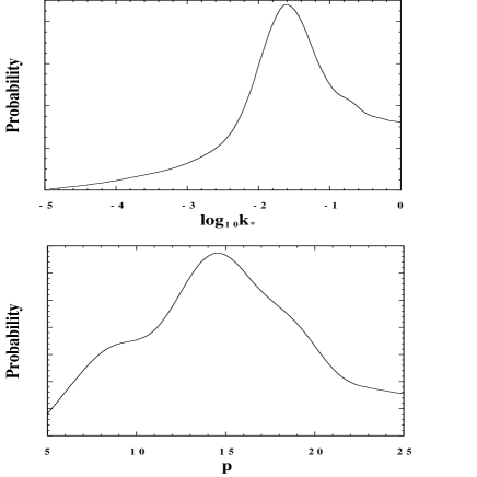
The probability distribution of the likelihood values of and are shown in Fig. 2. This corresponds to the mean likelihood analysis where the probability distribution of is assumed to be Gaussian, as (here is the minimum value of ). The best-fit critical scale corresponds to
| (18) |
in which case the spectrum changes from (7) to (12) around . The distribution of is consistent with the result of Huang:2003zp , obtained by using the WMAP data at the scale . Other best-fit values are found to be
| (19) |
, and
| (20) |
Since changes to scale-invariant for , the angular power spectrum exhibits a better fit compared to the standard case [compare curves (b) and (c) in Fig. 1]. This is an advantage of non-commutative inflation, which allows for the running of the spectral index, due to the existence of a cut-off momentum that arises from the stringy uncertainty relation. Note that using only the formula (7) leads to a power spectrum which is even more suppressed for low multipoles, as seen in Fig. 1 (a), but this is ruled out since becomes negative.
We can constrain the string length scale, , by using the above best-fit values. Since the two spectra (7) and (12) are interpolated at , we have
| (21) |
where we used the fact . The scale is chosen as in the numerical calculation of CAMB. Substituting the most likely values of , and in Eq. (21), one gets
| (22) |
which corresponds to a string length scale, . This result must be interpreted with care. It means that in the context of our postulated theoretical framework, the best fit value of is the above one. From Fig. 2 it is also clear that this value of is more likely only by a modest amount than the value .
We also considered the case where the cosmologically relevant scales are dominated by the spectrum (7), and obtained a similar constraint to (22) by utilizing the likelihood values of , and . Since in Eq. (21), the change of around the scale does not lead to any significant modification for the estimation of . The string length scale is mainly determined by the ratio . It is quite intriguing that space-time non-commutativity opens up the possibility to constrain the string scale by using the observational CMB data sets.
The largest scales correspond to the initial time with . Expanding the exact solution (11) around , we get
| (23) |
where
| (24) | |||||
| (25) |
This is a blue tilted spectrum for . The critical scale is much less than ; e.g., for , . As long as the spectra are characterized by (7) and (12) on the scales , Eq. (23) is not important, since it applies only well beyond , with . While the case (b) in Fig. 1 exhibits good agreement with the WMAP data, the scale-invariant spectrum (12) is not sufficient to explain significant loss of power around . The amplitude of the fluctuations tends to grow toward smaller multipoles due to the Sachs-Wolfe effect even in the scale-invariant case.
Instead we can consider a case where the spectrum around is characterized by (23). When , Eq. (23) can be written in the form
| (26) |
with . This corresponds to the case of an exponential cut-off in the spectrum analyzed in Contaldi ; Cline ; bfm , except for the absence of the tilted term, . In Contaldi ; Cline , the value is chosen, and the TT spectrum is shown to be suppressed for low multipoles. It is clear that is required for strong suppression on large scales (for example, see Fig. 1 in bfm for and ). Since is larger than unity in our case, for non-commutative inflation is restricted to be smaller than 1. Therefore, we do not have a significant suppression only around as long as we use the spectrum (23) with . Note, however, that the spectrum can be better fitted than the standard CDM model in power-law inflation.
IV Discussion
In this work we have found the best-fit parameters of a model of inflation based on space-time non-commutativity Brandenberger:2002nq when comparing to the recent WMAP spectrum of CMB anisotropies. The advantage of this approach is that one uses stringy phenomenology to modify inflationary perturbations, rather than imposing ad hoc modifications. The stringy corrections ensure that the model is not subject to the trans-Planckian problem of general inflationary models, since the physical wavenumbers of modes have an upper bound. At the same time, this feature means that high-energy stringy effects modify the large-scale perturbations rather than those on small scales, since large-scale modes are generated outside the Hubble radius and thus experience growth due to squeezing for less time than they do for . This model automatically predicts that at large angular scales the spectrum will be blue, thus providing a possible explanation for the observed lack of power at the quadrupole and octopole. Roughly speaking, requiring the correct location of the transition between blue and red spectrum in our model determines the string length scale, whereas the spectrum on smaller angular scales determines the best fit value of the power-law exponent .
Given that there are now a large number of possible explanations of the observed deficit of power on large angular scales, it would be of interest to look for special signals in our model not present in the other proposed theoretical explanations. Work on this subject is in progress. Note that our “determination” of the length scale assumes that our class of models is in fact correct, and that no secondary effects cause any deviations of the spectrum. The first point, in particular, is a major assumption to be justified.
We have for simplicity assumed power-law inflation. In this case is proportional to due to the time-independence of the small parameter, . Therefore, the spectrum of curvature perturbations is similar to that of gravitational waves, except for their amplitudes. The spectrum changes in general inflation models because of the time variation of . In particular, the running of the spectral index can be different from the one in power-law inflation. Although it may be in general difficult to obtain the spectrum of primordial curvature perturbations analytically, it will be interesting to extend our analysis to other inflationary models by using a numerical approach. This would allow the exciting possibility to place more generally applicable limits on the string length scale, in addition to limits on the value of more general inflationary model parameters.
Recently Cremonini , it was shown that a quantum deformation
of the wave equation on a cosmological background yields a
modified power spectrum analogous but not identical to
Eq. (7). It would be of interest to constrain the
region of parameter space in those models through a likelihood
analysis similar to what we have done here, since this can provide
a powerful tool to pick up a possible trans-Planckian effect and
to distinguish between different string inspired cosmological
models.
Acknowledgements
We are indebted to Antony Lewis for crucial advice and support in implementing and interpreting the likelihood analysis. S.T. is grateful to Bruce Bassett, Rob Crittenden and David Parkinson for useful discussions. R.B. thanks George Efstathiou for important advice. We also wish to acknowledge discussions with Stephon Alexander at the beginning of this project. S.T. acknowledges financial support from JSPS (No. 04942). R.M. is supported by PPARC. R.B. is supported in part by the US Department of Energy under Contract DE-FG02-91ER40688, TASK A.
References
-
(1)
A. H. Guth,
Phys. Rev. D 23, 347 (1981);
K. Sato, Mon. Not. Roy. Astron. Soc. 195, 467 (1981). -
(2)
R. H. Brandenberger and J. Martin,
Mod. Phys. Lett. A 16, 999 (2001);
J. Martin and R. H. Brandenberger, Phys. Rev. D 63, 123501 (2001). - (3) R. H. Brandenberger, hep-th/0210186.
-
(4)
L. Bergstrom and U. H. Danielsson,
JHEP 0212, 038 (2002);
X. Wang, B. Feng and M. Li, arXiv:astro-ph/0209242;
V. Bozza, M. Giovannini and G. Veneziano, JCAP 0305, 001 (2003);
C. P. Burgess, J. M. Cline, F. Lemieux and R. Holman, JHEP 0302, 048 (2003);
J. Martin and R. Brandenberger, hep-th/0305161;
C. P. Burgess, J. M. Cline and R. Holman, hep-th/0306079;
O. Elgaroy and S. Hannestad, astro-ph/0307011;
N. Kaloper and M. Kaplinghat, hep-th/0307016. - (5) A. Kogut et al., astro-ph/0302213.
- (6) D. N. Spergel et al., astro-ph/0302209.
- (7) L. Verde et al., astro-ph/0302218.
- (8) H. V. Peiris et al., astro-ph/0302225.
- (9) G. Efstathiou, astro-ph/0306431.
- (10) S. L. Bridle, A. M. Lewis, J. Weller and G. Efstathiou, astro-ph/0302306.
-
(11)
S. de Deo, R. R. Caldwell and P. J. Steinhardt, Phys. Rev. D67,
103509 (2003);
G. Efstathiou, astro-ph/0303127;
J. P. Uzan, A. Riazuelo, R. Lehoucq and J. Weeks, astro-ph/0303580. - (12) C. R. Contaldi, M. Peloso, L. Kofman and A. Linde, JCAP 0307, 002 (2003).
- (13) J. M. Cline, P. Crotty and J. Lesgourgues, astro-ph/0304558.
- (14) B. Feng and X. Zhang, astro-ph/0305020.
- (15) J. Yokoyama, Phys. Rev. D 59, 107303 (1999).
- (16) M. Kawasaki, M. Yamaguchi and J. Yokoyama, Phys. Rev. D 68, 023508 (2003).
- (17) M. Bastero-Gil, K. Freese and L. Mersini-Houghton, hep-ph/0306289.
-
(18)
T. Yoneya,
Mod. Phys. Lett. A 4, 1587 (1989);
M. Li and T. Yoneya, hep-th/9806240. - (19) S. Alexander, R. Brandenberger and J. Magueijo, Phys. Rev. D 67, 081301 (2003).
- (20) R. Brandenberger and P. M. Ho, Phys. Rev. D 66, 023517 (2002).
- (21) Note that a different type of non-commutativity in inflation is possible fkm , with qualitatively different features to those considered here. Non-commutativity is applied on the sphere, rather than the real spacetime non-commutativty considered here. Modes are set to be absent at all times if they are inconsistent with the non-commutativity constraint at the time of Hubble radius crossing. By contrast, in our case modes are produced if they initially do not satisfy the constraint.
- (22) M. Fukuma, Y. Kono and A. Miwa, hep-th/0307029.
- (23) The reason is that these modes undergo a shorter period of squeezing than they do according to the standard calculations.
- (24) Q. G. Huang and M. Li, JHEP 0306, 014 (2003).
- (25) V. F. Mukhanov, H. A. Feldman and R. H. Brandenberger, Phys. Rept. 215, 203 (1992).
- (26) http://camb.info/
-
(27)
A. Lewis, A. Challinor and A. Lasenby,
Astrophys. J. 538, 473 (2000);
A. Lewis and S. Bridle, Phys. Rev. D 66, 103511 (2002). - (28) http://lambda.gsfc.nasa.gov/
- (29) T. Pearson et al., astro-ph/0205388.
- (30) K. Grainge et al., astro-ph/0212495.
- (31) C. L. Kuo et al., astro-ph/0212289.
- (32) S. Cremonini, hep-th/0305244.