Multi-wavelength Cosmological Simulations of Elliptical Galaxies

Abstract

We study the chemodynamical evolution of elliptical galaxies and their X-ray and optical properties using high-resolution cosmological simulations. Our Tree N-body/SPH code includes a self-consistent treatment of radiative cooling, star formation, supernovae feedback, and chemical enrichment. We present a series of ${\rm\Lambda}$CDM cosmological simulations which trace the spatial and temporal evolution of abundances of heavy element in both the stellar and gas components of galaxies. A giant elliptical galaxy formed in the simulations is quantitatively compared with the observational data in both the X-ray and optical regime. X-ray spectra of the hot gas are constructed via the use of the vmekal plasma model, and analysed using XSPEC with the XMM EPN response function. Optical properties are derived by the population synthesis for the stellar component. We find that radiative cooling is important to interpret the observed X-ray luminosity, temperature, and metallicity of the hot gas of elliptical galaxies. However, this cooled gas also leads to excessive star formation at low redshift, and therefore results in underlying galactic stellar populations which are too blue with respect to observations. Time variation and radial dependence of X-ray properties and abundance ratios, such as [O/Fe] and [Si/Fe], of the X-ray emitting hot gas are also discussed.

1 Introduction

Historically, galactic astronomy was based on optical observation. At optical wavelengths, general properties especially for nearby elliptical galaxies are well studied. For example, the various scaling relations for nearby elliptical galaxies, such as the Colour-Magnitude Relation (CMR: e.g. Sandage, 1972; Aaronson, Persson, & Frogel, 1981; Bower, Lucey, & Ellis, 1992a, b) and fundamental plane (e.g. Djorgovski & Davis, 1987; Dressler et al., 1987), provide strong constraints on the formation paradigm of elliptical galaxies. On the other hand, progressive developments of telescopes and instruments have opened up other wavelengths, such as X-ray and radio, and made it possible to observe galaxies at those wavelengths with similar or even higher sensitivity and resolution than those in the optical observations. As a result, those multi-wavelength observations throw a new light on the study of the formation and evolution of galaxies.

As for elliptical galaxies, the discovery of an X-ray emitting hot interstellar medium (ISM) has dramatically renewed the view of their physical properties and formation history (e.g. Forman et al., 1979; Forman, Jones, & Tucker, 1985). The optical observation represents mainly the properties of stellar component. On the other hand, X-ray observations offer a unique tool for the study of the hot gas component. Since there is little cold gas in elliptical galaxies (e.g. Bregman, Hogg, & Roberts, 1992; Edge, 2001; Georgakakis et al., 2001), those two are the major components of elliptical galaxies. Therefore, any successful scenario of elliptical galaxy formation must explain both X-ray and optical observation.

The aim of this paper is to present our first attempt to construct a successful self-consistent cosmological simulation of elliptical galaxies whose properties are consistent with both X-ray and optical observations. To this end, we carry out a series of high-resolution cosmological simulations using our galactic chemodynamical evolution code (GCD+: Kawata & Gibson, 2003). The code is a three-dimensional tree N-body/smoothed particle hydrodynamics (SPH) code which incorporates self-gravity, hydrodynamics, radiative cooling, star formation, supernovae (SNe) feedback, and metal enrichment. GCD+ takes account of the chemical enrichment by both SNe II and SNe Ia, and mass-loss from intermediate mass (IM) stars, and follows the evolution of the abundances of several chemical elements in both gas and stellar components. Based on the plasma model for hot gas and single stellar population (SSP) for stars, this self-consistent chemodynamical treatment allows us to derive the X-ray and optical spectral energy distribution (SED) for the simulation end-products with minimal assumptions. Taking advantage of this, we compare these results for an elliptical galaxy in our simulation with the observational data at X-ray and optical wavelength directly and quantitatively, and discuss the physical processes of the formation and evolution of elliptical galaxies.

In the X-ray observation, we focus on the well-studied observational values of luminosity, $L_{X}$, temperature, $T_{X}$, and iron abundance, [Fe/H]_X. In observed clusters of galaxies, there is well-known ${L_{X}}-{T_{X}}$ relation, ${L_{X}}\propto{T_{X}}^{b}$: $b=2.5-3$ (e.g. Edge & Stewart, 1991; Xue & Wu, 2000). On the other hand, the simple spherical top-hat density perturbation theory predicts that the virial temperature and density of a cluster with mass $M$ follow $T\propto M^{2/3}(1+z)$ and $\rho\propto(1+z)^{3}$ at a redshift of $z$ (e.g. Padmanabhan, 1993). At typical cluster temperatures ($T>2$ keV), free-free emission dominates the cooling process, and the X-ray luminosity is expected to be $L_{X}\propto M\rho T^{1/2}$. If all clusters followed this simple scaling low, we would expect $L_{X}\propto T^{2}$ at a fixed redshift, which is a significantly shallower slope than that observed. Recently, the ${L_{X}}-{T_{X}}$ relation for groups of galaxies has also been examined, and is revealed to have much steeper slope, $b\sim 5$, than that for clusters of galaxies (e.g. Helsdon & Ponman, 2000; Xue & Wu, 2000). Thus, in lower mass systems, the agreement between the simple theoretical prediction and the observations becomes even worse, i.e., the X-ray luminosity of low-temperature system is unexpectedly small. Ponman, Cannon, & Navarro (1999) calculated the specific entropy of the gas for observed groups and clusters, and found an “entropy floor” of $S\equiv T/n_{e}^{2/3}\sim 100h^{-1/3}$ keV cm^-2, where $n_{e}$ is the electron number density. This entropy floor reduces the X-ray luminosity by lowering the gas density progressively more in smaller system, and hence reproduces the steep $L_{X}-T_{X}$ relations seen in groups.

One approach to explain this entropy floor is “pre-heating” of the gas before the system collapses (Evrard & Henry, 1991; Kaiser, 1991). Lloyd-Davies, Ponman, & Cannon (2000) estimated that a pre-heating temperature of $\sim$0.3 keV is required to explain the entropy floor, if the energy is injected well before cluster collapse. If energy injection takes place internally, i.e. within collapsed halos, more energy is required, $\sim 1-3$ keV (Loewenstein, 2000; Wu, Fabian, Nulsen, 2000; Bower et al., 2001). Although the source of the pre-heating is still unclear, this scenario is also supported by numerical simulations which take into account the dynamical evolution of the system (e.g. Navarro, Frenk, & White, 1995; Muanwong et al., 2002). An alternative mechanism to explain the entropy floor is radiative cooling. Bryan (2000) pointed out that smaller systems, such as groups, have converted more of their gas into galaxies than larger systems, and the gas that goes to form the galaxies was lower in entropy preferentially, thus raising the mean entropy of the gas that remains. Voit & Bryan (2001) further argued that cooling removes low-entropy gas during the formation of cluster galaxies, and showed that this mechanism naturally explains an entropy floor of $\sim$ 100 keV cm^-2. Hydrodynamic cosmological simulations also support these analytic arguments (e.g. Pearce et al., 2000; Muanwong et al., 2001, 2002; Davé, Katz, & Weinberg, 2002; Valdarnini, 2003).

The size of the potential well of elliptical galaxies corresponds to the low mass end of the groups observed in the above studies. Matsushita, Ohashi, & Makishima (2000, MOM00) showed that the X-ray luminosities of elliptical galaxies are well below that expected from the extrapolation of the cluster $L_{X}-T_{X}$ relation. Therefore, the entropy floor seems to be still active on the scale of elliptical galaxies. However, the above theoretical work focuses on larger systems, such as groups and clusters. On the elliptical galaxy scale, we must take into account details of complex radiative cooling processes, star formation, as well as SNe feedback at the formation epoch and during the long time evolution of the system (Mathews & Loewenstein, 1986; Hattori, Habe, & Ikeuchi, 1987). These processes were simplified in the above theoretical studies, or were difficult to follow due to the resolution limit of numerical simulations. Thus, to examine the $L_{X}-T_{X}$ relation for elliptical galaxies is a challenging problem, and this paper will shed light on this issue.

X-ray observation also provides the chemical composition of the hot gas, which should contain a fossil record of past history of the elliptical galaxy evolution, because stellar mass-loss products and SNe ejecta are expected to be accumulated in the hot gas. The standard SNe and stellar mass-loss rates predict the metallicity of the hot gas to be several times higher than the solar value (e.g. Loewenstein & Mathews, 1991; Arimoto et al., 1997; Brighenti & Mathews, 1999). However, previous measurements of ISM of elliptical galaxies with ASCA have shown that the iron abundance is less than the solar abundance (Awaki et al., 1994; Loewenstein et al., 1994; Matsumoto et al., 1997; Matsushita, Ohashi, & Makishima, 2000). This discrepancy between the theoretical predictions and observations is called the “iron discrepancy” (Arimoto et al., 1997). X-ray iron abundances remain a controversial issue. Recently, Buote & Fabian (1998); Buote (1999, 2002) claimed that some X-ray luminous galaxies have roughly solar abundance, employing a multi-temperature plasma model. However, even these observed abundances are still lower than the theoretical prediction. Also, high-resolution spectra taken with Reflecting Grating Spectrometers (RGS) on board XMM-Newton show less than solar abundance (Xu et al., 2002; Sakelliou et al., 2002; Tamura et al., 2003).

To solve this iron discrepancy, a couple of scenarios have been suggested. Using a chemodynamical evolution model, Bekki (1998) showed that the metallicity of the ISM (especially in the outer regions) becomes lower than that of the stellar component in some elliptical galaxies formed by gas-rich disk-disk galaxy mergers, because less metal-enriched ISM is tidally stripped away and surrounds its merger remnant. Considering evolution after the galaxy formed, using a multi-phase chemical evolution model, Fujita, Fukumoto, & Okoshi (1996, 1997) suggested that X-ray emitting hot gas is hardly enriched, because the enriched gas cools more easily and drops out of the hot gas phase. Unfortunately, there is no study following the chemodynamical evolution of elliptical galaxies from the epoch of their complex hierarchical formation to the present, based on the self-consistent cosmological simulation. Thus, our study would be important to test those scenarios in the context of the cosmological evolution.

From the previous studies above, radiative cooling is apparently considered to be a key mechanism in understanding the X-ray properties, such as $L_{X}$, $T_{X}$, and [Fe/H]_X, of elliptical galaxies. Therefore, we first examine the effects of radiative cooling, comparing the results of simulations with and without radiative cooling. Pre-heating is also an interesting mechanism, although the origin of the pre-heating is unclear. Hence, we also consider the effect of SNe feedback which is one of candidates of the source of the pre-heating as well as the internal heating within the collapsed halo (Mathews & Loewenstein, 1986; Hattori, Habe, & Ikeuchi, 1987; Ciotti et al., 1991; Ponman, Cannon, & Navarro, 1999; Lloyd-Davies, Ponman, & Cannon, 2000; Wu, Fabian, Nulsen, 2000; Bower et al., 2001). In this paper, we would like to clarify the effects of radiative cooling and SNe feedback on the X-ray properties of elliptical galaxies, such as $L_{X}$, $T_{X}$, and [Fe/H]_X.

As mentioned above, we must explain not only the X-ray but also optical properties. Although the previous studies pointed out the importance of radiative cooling, they did not answer where the cooled gas has gone. It would be natural to expect that such cooled gas would be the source of successive star formation. However, the optical observations, such as the CMR, provide a strong restriction on such recent star formation. Therefore, we test the CMR of the stellar component of the simulation end-products as well. We will show that this test gives a serious constraint on the theoretical model.

The outline of this paper is as follows. Details of our code, numerical simulation model, and analysis of X-ray and optical properties are described in Section 2. In Section 3, we show the results, and compare the simulation results with the observational data in both the X-ray and the optical regime. Finally, we present a discussion and conclusions in Section 4. Throughout this paper, we adopt for the solar abundance the “meteoric” values in Anders & Grevesse (1989).

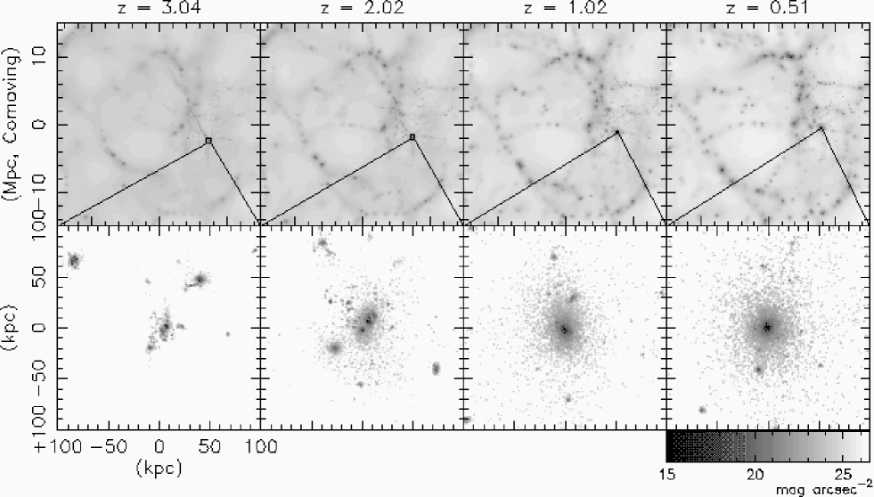
Figure 1: Dark matter density map of a portion of the 43 Mpc (comoving) simulation volume (upper panels), and predicted $I$-band image (physical scale) of the target galaxy (lower panels), over the redshift range $z$=3.0 to $z$=0.5.

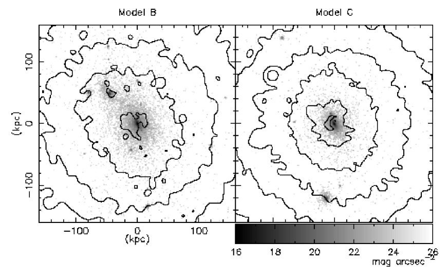
Figure 2: R band image of the target galaxy for Models B (left) and C (right) at z=0. Overlaid contours show X-ray surface brightness.

2 Methods

2.1 The Galactic Chemodynamical Evolution Code

Our simulations were carried out using GCD+, our original galactic chemodynamical evolution code. Details of the code are presented in Kawata (1999) and Kawata & Gibson (2003). The code is essentially based on TreeSPH (Hernquist & Katz, 1989; Katz, Weinberg, & Hernquist, 1996), which combines the tree algorithm (Barnes & Hut, 1986) for the computation of the gravitational forces with the SPH (Lucy, 1977; Gingold & Monaghan, 1977) approach to numerical hydrodynamics. The dynamics of the dark matter (DM) and stars is calculated by the N-body scheme, and the gas component is modeled using SPH. It is fully Lagrangian, three-dimensional, and highly adaptive in space and time owing to individual smoothing lengths and individual time steps. Moreover, it includes self-consistently almost all the important physical processes in galaxy formation, such as self-gravity, hydrodynamics, radiative cooling, star formation, SNe feedback, and metal enrichment.

Radiative cooling which depends on the metallicity of the gas (derived with MAPPINGSIII: Sutherland & Dopita, 1993) is taken into account. The cooling rate for a gas with solar metallicity is larger than that for gas of primordial composition by more than an order of magnitude. Thus, the cooling by metals should not be ignored in numerical simulations of galaxy formation (Käellander & Hultman, 1998; Kay et al., 2000).

We stress that GCD+ takes account of energy feedback and metal enrichment by both SNe II and SNe Ia, and metal enrichment from IM stars (see Kawata & Gibson, 2003, for details). The code calculates the event rates of SNe II and SNe Ia, and the yields of SNe II, SNe Ia, and IM stars for each star particle at every time step, considering the Salpeter (1955) initial mass function (IMF: mass range of 0.1$\sim$60 ${\rm M_{\rm\sun}}$) and metallicity dependent stellar lifetimes (Kodama, 1997; Kodama & Arimoto, 1997). We assume that each massive star ($\geq 8\ {\rm M_{\rm\sun}}$) explodes as a Type II supernova. The SNe Ia rates are calculated using the model proposed by Kobayashi, Tsujimoto, & Nomoto (2000). The yields of SNe II, SNe Ia, and IM stars are taken from Woosley & Weaver (1995), Iwamoto et al. (1999), and van den Hoek & Groenewegen (1997), respectively. The mass, energy, and heavy elements ejected from star particles are smoothed over the neighbouring gas particles using the SPH smoothing algorithm. For example, when the $i$-th star particle ejects the mass of $M_{\rm SN,{\it i}}$, the increment of the mass of the $j$-th neighbour gas particle is given by

$$\Delta{M_{\rm SN,{\it j}}}=\frac{m_{j}}{\rho_{{\rm g},i}}{M_{\rm SN,{\it i}}}W(r_{ij}/h_{i}),$$ (1)

where

$$\rho_{{\rm g},i}=\langle\rho_{\rm g}(\mbox{\boldmath$x$}_{i})\rangle=\sum_{j\neq i}m_{j}W(r_{ij}/h_{i}),$$ (2)

and $W(x)$ is an SPH kernel (Kawata & Gibson, 2003). The simulation follows the evolution of the abundances of several chemical elements (¹H, ⁴He,¹²C, ¹⁴N, ¹⁶O, ²⁰Ne, ²⁴Mg, ²⁸Si, ⁵⁶Fe, and Z, where Z means the total metallicity). The self-consistent calculation of both chemical (especially including the metal enrichment from SNe Ia and IM stars, which were often ignored in previous chemodynamical simulations) and dynamical evolution by GCD+ makes it possible for us to analyse the chemical and physical properties for both the gas and stellar components, which is essential for this study,

2.2 Cosmological Simulation and the Target Galaxy

Using GCD+, we have carried out a series of high-resolution simulations within the adopted standard $\Lambda$-dominated cold dark matter ($\Lambda$CDM) cosmology ($\Omega_{0}$=0.3, $\Lambda_{0}$=0.7, $\Omega_{\rm b}$=0.019$h^{-2}$, $h$=0.7, and $\sigma_{8}$=0.9). We use the multi-resolution technique, to achieve high-resolution in the interesting region, including the tidal forces from the large scale structures. The initial conditions for the following simulations are constructed using the public software “GRAFIC2” (Bertschinger, 2001). All our simulations use isolated boundary conditions. Initially, we perform a low-resolution N-body simulation of a comoving 30$h^{-1}$ Mpc diameter sphere. Mean separation of the particles is 30$h^{-1}$/48 Mpc. The mass of each particle is $2.90\times 10^{10}{\rm M_{\sun}}$, and a fixed physical softening of 18.0 kpc is applied.

At redshift $z=0$, we selected an 11.6 Mpc diameter spherical region, which contains a few galaxy-sized DM halos. We trace the particles which fall into the selected region back to the initial conditions at $z=38.6$, and identify the volume which consists of those particles. Within this arbitrarily shaped volume, we replace the low resolution particles with 64 times less massive particles. The initial density and velocities for the less massive particles are self-consistently calculated by GRAFIC2, taking into account the density fields of a lower resolution region. Finally, we re-run the simulation of the whole volume (30$h^{-1}$ Mpc sphere), including the gas dynamics, cooling, and star formation. The gas component is included only within the high-resolution region. The surrounding low-resolution region contributes to the high-resolution region only through gravity. The mass and softening length of individual gas (DM) particles in the high-resolution region are $5.86\times 10^{7}$ ($3.95\times 10^{8}$) ${\rm M}_{\rm\sun}$ and 2.27 (4.29) kpc, respectively.

At $z=0$, using the friends-of-friends technique, we found 5 stellar systems which consist of more than 2000 star particles. The largest stellar system has an elliptical galaxy like morphology, and the kinematics shows that the system is supported mainly by velocity dispersion rather than rotation (the ratio of the max rotational velocity to the max velocity dispersion, $V/\sigma\sim 0.7$). We chose this system as the target galaxy for this study. The rest of the paper focuses on this target galaxy. The total virial mass of this galaxy is $M_{\rm vir}\sim 2\times 10^{13}$ ${\rm M_{\sun}}$, similar in size to that of NGC 4472, a bright elliptical galaxy in the Virgo Cluster. The virial mass is defined as the mass within the virial radius, $r_{\rm vir}$, which is the radius of a sphere containing a mean density of $178\Omega_{0}^{0.45}$ times the critical values, $\rho_{\rm crit}=3{\rm H_{0}}/8\pi G$, following Eke, Navarro, & Frenk (1998).

As described in Section 1, we are interested in the effect of radiative cooling and SNe feedback. We carry out a series of simulations with this initial condition, using the following three models. Model A is an adiabatic (i.e. no cooling) model; Model B includes cooling and weak feedback; Model C mimics Model B, but incorporates stronger feedback. Model B assumes that each SN yields the energy of $10^{50}$ ergs, but Model C adopts the energy of $10^{52}$ ergs. The energy in Model C is unrealistically higher than the canonical value ($10^{51}$ ergs). We use this model as an extreme comparison case, to see the dependence of the strength of the SNe feedback more clearly. Also note that we assume that all kinetic energy of SNe is turned into thermal energy on a scale less than our resolution limit, and thus only the thermal energy of SNe is available to affect the surrounding gas of our resolution.

Fig. 1 shows the morphological evolution of DM in a central portion of the simulation volume, and the evolution of the stellar component in a 200 kpc region centred on the target galaxy for Model B. The lower panels correspond to the $I$ band (in observed frame) image of the target galaxy, which is made using population synthesis techniques as explained in the next section. We take into account the K-correction, but do not consider any dust absorption. The galaxy forms through conventional hierarchical clustering between redshifts $z$=3 and $z$=1; the morphology has not changed dramatically since $z$=1. Fig. 2 displays the final (at $z=0$) $R$ band image (gray scale image) and X-ray surface brightness profile (contours) for Models B and C. The target galaxy is relatively isolated, with only a few low-mass satellites remaining at $z$=0. Model parameters and final basic properties for each model are summarised in Table 1.

Table 1: Model Parameters.

	energy per SN	$r_{\rm vir}$	Mass within $r_{\rm vir}$ (M☉)			Number of Particles
Name	(ergs)	(kpc)	Gas	DM	Star	Gas	DM	Star
A	$-$	821	$2.14\times 10^{12}$	$1.60\times 10^{13}$	0	36457	40492	0
B	$10^{50}$	821	$1.45\times 10^{12}$	$1.60\times 10^{13}$	$1.08\times 10^{12}$	21136	40454	18966
C	$10^{52}$	825	$1.83\times 10^{12}$	$1.62\times 10^{13}$	$6.02\times 10^{11}$	30765	41036	10782

2.3 Analysis

For all the models, we examine both the resulting X-ray and optical properties, comparing them quantitatively with observation. The following sections describe how we derived synthesised spectra in both X-ray and optical bands from the simulation results.

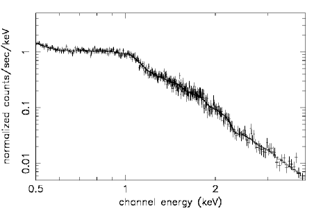
Figure 3: Synthesised X-ray Spectrum (error-bars) and vmekal model fit (solid line).

2.3.1 X-ray Synthesised Spectrum and Fitting

To derive the X-ray spectrum, we need to know the density, temperature, and abundances of heavy elements for the gas component. Due to our chemodynamical evolution code, the gas particles in our simulations carry with them knowledge of those physical and chemical properties. Using the XSPEC ver.11.1.0 vmekal plasma model (Mewe, Gronenschild, & van den Oord, 1985; Mewe, Lemen, & van den Oord, 1986; Kaastra, 1992; Liedahl Osterheld, & Goldstein, 1995), we derive the X-ray spectra for each gas particle, and synthesise them within the assumed apertures. We next generate “fake” spectra with the response function of the XMM EPN detector, assuming an exposure time (40 ks) and target galaxy distance (17 Mpc). Finally, our XSPEC fitting of this fake spectrum provides the X-ray weighted temperatures and abundances of various elements. In this section, we describe the process of this analysis in detail.

First, we generate the X-ray spectrum for each gas particle. We use the subroutine of the XSPEC vmekal model. Input parameters of the vmekal model are the hydrogen number density, temperature, and abundances of He, C, N, O, Ne, Na, Mg, Al, Si, S, Ar, Ca, Fe, and Ni, with respect to the hydrogen abundance. The temperature for each particle are given directly from the simulation output. The hydrogen number density is derived by the gas density times the hydrogen abundance divided by the mass of hydrogen atom, i.e. the proton mass. Due to the limitation of the size of memory, our numerical simulation follows the abundance evolution of only ¹H, ⁴He,¹²C, ¹⁴N, ¹⁶O, ²⁰Ne, ²⁴Mg, ²⁸Si, ⁵⁶Fe. Simply, we assume the abundance of these elements with respect to ¹H is the same as the total abundance of all isotopes with respect to the total (¹H and ²H) hydrogen abundance, e.g. ${}^{16}{\rm O}$/${}^{1}{\rm H}$=${\rm O(=^{16}O+^{17}O+^{18}O)}$/${\rm H(=^{1}H+^{2}H)}$. For the elements whose abundances are not calculated in our simulation, we assume [Na/H]$=$[Al/H]$=$[O/H], [S/H]$=$[Ar$/$H]$=$[Ca$/$H]$=$[Si/H], and [Ni/H]$=$[Fe/H], here [X/H] $=\log_{10}({\rm X}/{\rm H})-\log_{10}({\rm X}_{\sun}/{\rm H}_{\sun})$. This assumption should not be an issue, because we use the same assumption when we fit the synthesised spectrum, as described later. Finally, we generate the spectrum for each gas particle within the energy range between 0.1 and 20 keV with 1800 bins, using the vmekal model.

To compare our results with the X-ray properties observed within a certain radius, we assume an aperture size. The X-ray fluxes for all the gas particles within the assumed apetrure radius are added up in each bin, and the synthesised spectrum is stored as a FITS file to enable XSPEC to read it as a model using atable command. Next, we make “fake” spectrum using fakeit command in XSPEC. In this paper, we suppose the observation by EPN detector on XMM-Newton, and the distance of the target galaxy is 17 Mpc. We use epn_ff20_sY9_thin.rmf for the EPN response file, and adopt 40 ks exposure time. Any absorption component or background are not taken into account. We binned the spectra to achieve at least 25 counts per bin, using “grppha” tool of HEASOFT ver.5.1. Fig. 3 shows an example of fake spectrum with $R=35$ kpc aperture for Model B.

Finally, using XSPEC, the generated fake spectrum is fitted by vmekal model within the energy range between 0.5 and 4 keV. As mentioned above, here we assume [Na/H]=[Al/H]=[O/H], [S/H]=[Ar/H]=[Ca/H]=[Si/H], and [Ni/H]=[Fe/H]. We fix the values of [He/H], [C/H], and [N/H] to be solar, i.e. zero, because those abundances do not affect the X-ray spectrum within the energy range which we use. Consequently, the free parameters for the fitting are the temperature and abundances of [O/H], [Ne/H], [Mg/H], [Si/H], and [Fe/H]. As shown later, except for Model A, two temperature vmekal models provide a better fit than one temperature models, irrespective of the aperture. In a two temperature model, we assume that the hot and cold components have the same abundances, to reduce the number of fitting parameters. The solid line in Fig. 3 shows the best fit two temperature vmekal model for the fake spectrum of Model B with an aperture $R=35$ kpc. For Model A, we set the metal abundance to be zero, i.e. [X/H]$=-\infty$, because, as there are no stars, no metals are produced, and find that a one temperature model can fit the spectrum very well. Such spectrum fitting gives us the X-ray weighted temperature, and the abundances of various elements.

Due to this analysis, we take into account the line emissions, and the energy range in fitting. This is more sophisticated way than a simple Bremsstrahlung-based model, where X-ray luminosity is assumed to be proportional to $\rho^{2}T^{1/2}$, which is conventionally used in numerical simulation studies of X-ray properties of clusters of galaxies (e.g. Navarro, Frenk, & White, 1995). Some previous studies used mekal model of XSPEC (e.g. Mathiesen & Evrard, 2001; Toft et al., 2002) or Raymond & Smith (1977) model (e.g. Katz & White, 1995; Muanwong et al., 2002) to derive the X-ray properties. Unfortunately, they fixed the metallicity to be the assumed value, because of the lack of information about chemical evolution, and they did not do any fitting of the generated spectrum. Fujita, Fukumoto, & Okoshi (1996, 1997) used meka model of XSPEC to derive the X-ray spectrum from the results of their one-dimensional chemical evolution model, and get the temperature and abundances by fitting the spectrum using XSPEC. However, they assumed the solar abundance pattern, i.e. [Fe/H]=$\log(Z/Z_{\sun})$, [X/Fe]=0, $Z$ is the total metal (elements heavier than He) abundance, and $Z_{\sun}$ is the solar abundance. Thus, the combination of our chemodynamical simulation and this analysis offers a higher level comparison between theoretical models and observational data than that in the previous studies. The dependence of the results on the analysis method is briefly discussed in Section 3.3.

In the following sections, we compare the simulation results with the X-ray observational data in MOM00. MOM00 measured the various X-ray properties, such as luminosity, temperature, metallicity, within an aperture radius of four times the $B$-band half-light radius. Unfortunately neither the half-light radius nor the optical luminosity of our models agree with the observed ones, because of a large population of young stars in the central part of the simulated galaxy (see Section 3.2 for details). Since we cannot fix the aperture using the same way as the observation due to this problem, we show the results with different apertures, and discuss the effects of aperture. For this purpose, 20 kpc and 35 kpc radius apertures are used. The former one roughly corresponds to four times the $B$ band half-light radius for the simulation end-products, when the light from young ($t_{\rm age}<8$ Gyr) stars are ignored. The latter one is similar to four times the $B$ band half-light radius of NGC 4472 ($r_{\rm h}\sim 8.5$ kpc). These apertures are applied to the projected distribution of the gas particles within the virial radius of the target galaxy at $z=0$. We use an arbitrary direction for projection, and the same projection is used when we derive the optical properties. We have checked that the results we show in this paper do not depend on the direction of the projection.

In this paper, we show the X-ray luminosity in the 0.5–10 keV pass band, because MOM00 showed the X-ray flux in this pass band. We focus on the X-ray emission from the hot ISM. The X-ray spectrum derived with the above analysis is an idealised spectrum from the hot ISM, because the observed X-ray flux comes from not only the hot ISM but also the background and the point sources, such as X-ray binaries. MOM00 carefully reduced the background, and also estimated the flux of the hard component which is considered to come from low-mass X-ray binaries. We assume that the flux of the soft component measured in MOM00 would be dominated by the contribution from the hot ISM, and use them in the following section. Nevertheless, it is important for this type of study to identify the X-ray sources, and evaluate the X-ray flux from the hot ISM correctly using high spatial and spectral resolution observation (Sarazin, Irwin, & Bregman, 2001).

2.3.2 Optical Population Synthesis

The optical photometric properties which are examined in this paper are derived using the same procedure as that used and described in Kawata (2001a, b). Here, we briefly describe this procedure. In our simulations, the star particles each carry their own age and metallicity “tag”, due to the self-consistent calculation of the chemodynamical evolution. This enables us to generate an optical-to-near infrared SED for the target galaxy, when combined with our population synthesis code adopting the SSP of the public spectrum and chemical evolution code, KA97 (Kodama, 1997; Kodama & Arimoto, 1997). It is worth noting that our simulation assumes the same shape and mass range of IMF and the same lifetime of stars as those assumed in the SSPs provided by KA97. Here, the SED of each star particle is assumed to be that of an SSP, i.e. a coeval and chemically homogeneous assembly of stars. Since the observational data which our results should be compared with provide the luminosity distribution projected onto a plane, we have to derive the projected distribution of the SED from the three-dimensional distribution of star particles. Finally, we obtain the images projected in the direction used in the X-ray analysis. For example, Fig. 2 shows the $R$-band images (gray scale image) for Models B and C, where a 1000 $\times$ 1000 pixel mesh is chosen to span a square region of side 320 kpc, and the flux of each star particle is smoothed using a gaussian filter with the filter scale of 1/4 of the softening length of the star particle. These images provide similar information to the imaging data obtained in actual observations. Thus, we can obtain various photometric properties from these images in the same way as in the analysis of observational imaging data. In the following analysis, we use images similar to the ones displayed in Fig. 2, but employing a 750 $\times$ 750 pixel mesh to span a squared region of side 100 kpc. The global photometric properties, such as the total luminosity and the colours, are obtained from the projected image data. In this paper, we focus on the colour and total magnitude of the target galaxy. For simplicity, we assume that the luminosity within an aperture raius of 50 kpc is the total luminosity. The colours are measured using the same aperture size as the observation which we compare with. These optical properties are discussed in Section 3.2.

Table 2: Model Results of X-ray Spectrum Fitting.

	Aperture $R<20$ kpc
	$L_{X}$	Fe/H	$kT_{1}$	$kT_{2}$	EM1/EM2	$\chi^{2}/\mu$	N${}_{\rm g}(R)$	N${}_{\rm g,hot}(R)$
Name	(1041 erg s-1)	(solar)	(keV)	(keV)
A	30.0	0.0	$0.45^{+0.00}_{-0.00}$	$-$	$-$	531.9/511	1607	1606
B	0.333	$0.17^{+0.04}_{-0.03}$	$1.52^{+0.10}_{-0.05}$	$0.73^{+0.09}_{-0.07}$	$0.323^{+0.103}_{-0.072}$	260.5$/$273	245	146
C	2.87	$0.21^{+0.01}_{-0.01}$	$1.22^{+0.02}_{-0.01}$	$0.47^{+0.03}_{-0.03}$	$0.169^{+0.013}_{-0.010}$	479.1$/$486	438	372
	Aperture $R<35$ kpc
Af	47.1	0.0	$0.45^{+0.00}_{-0.00}$	$-$	$-$	478.9/543	3657	3654
B	0.710	$0.12^{+0.02}_{-0.02}$	$1.39^{+0.08}_{-0.07}$	$0.67^{+0.03}_{-0.04}$	$0.451^{+0.103}_{-0.093}$	311.7$/$347	542	411
C	5.48	$0.12^{+0.01}_{-0.01}$	$1.16^{+0.01}_{-0.01}$	$0.54^{+0.03}_{-0.02}$	$0.229^{+0.015}_{-0.011}$	549.7$/$572	1166	1058

Figure 4: Comparison of the simulated and observed (crosses with error-bars) ${L_{X}-T_{X}}$ relations. The observational data are taken from MOM00. The triangle/circle/square indicates the predictions of Model A/B/C. The open (filled) symbols denote the values evaluated within the radius of 35 (20) kpc. The dashed line represents the relation obtained from the adiabatic simulation of Muanwong et al. (2001). Open diamond shows the value for Model A evaluated by the same method as Muanwong et al. (2001).

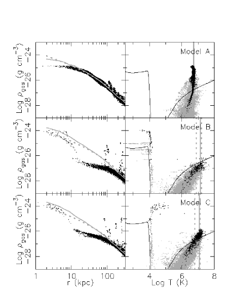
Figure 5: Density vs radius (left) and density vs temperature (right) distributions of gas particles for Model A (upper), Model B (middle), and Model C (bottom). In the left panels, the gray thick solid lines show the DM density profiles, and the gray dotted lines show the NFW profiles (see text for details). The DM densities are scaled by $\Omega_{b}/(\Omega_{0}-\Omega_{b})$ to compare with the gas density profiles. The solid curves in the right panels separate the region where the cooling time (${\rm t_{cool}}$) is shorter (upper region) and longer than the Hubble time (${\rm t_{H}}$). In the right panels, the black (gray) dots represent the particle within (outside of) the projected radius of 35 kpc. The vertical gray solid lines show the mean temperatures weighted by emission measure of the two temperature components (described by dotted lines) obtained by the spectrum fitting. Since the spectrum for Model A is fitted by one component, only the solid line is appeared.

3 Results

First, we discuss the global properties of the target galaxy in different models. Section 3.1 examines the X-ray properties, and compares them with the observed X-ray luminosity$-$temperature (${L_{X}-T_{X}}$) relation and X-ray luminosity$-$iron abundance ($L_{X}-{\rm[Fe/H]}_{X}$) relation of elliptical galaxies in MOM00. Section 3.2 discusses the optical properties of the target galaxy. Here, we focus on the CMR, which is well-established by the previous observation, and gives strong constraints on the stellar population of the elliptical galaxy. In Section 3.3, we mention the X-ray properties at different radii, i.e. the radial gradients. Then, the dependence of the derived X-ray properties on the analysis method is briefly argued. We also show time variation of X-ray properties in Section 3.4. Finally, abundance ratios of the X-ray emitting hot gas are discussed in Section 3.5.

3.1 X-ray Properties at the Central Region

3.1.1 ${L_{X}-T_{X}}$ Relation

Fig. 4 shows the predicted ${L_{X}-T_{X}}$ relation for the three models at $z=$0; crosses with error-bars represent the observational data from MOM00. As shown in Table 2 and Section 2.3.1, except for Model A, the two temperature vmekal model is applied to fit the synthesised X-ray spectrum. Thus, Fig. 4 plots the mean temperatures weighted by the emission measure of the two components for Models B and C.

The adiabatic model (Model A) appears incompatible with the observational data due to its excessive luminosity and low temperature. The X-ray luminosity is too high, and/or the X-ray weighted temperature is too low. The dashed line of Fig. 4 shows the ${L_{X}-T_{X}}$ relation obtained from the adiabatic cosmological simulation of Muanwong et al. (2001). The result of Model A is rather close to this line than the observational data. Note that Muanwong et al. (2001) derive the luminosity with a simple analytic formula, and do not apply any aperture or X-ray pass band, i.e. the summation of the cooling rates for all the gas particles with temperature larger than 10⁵ K. Thus, their luminosity means the bolometric luminosity, which is the reason why the luminosity for Model A is smaller than the dashed line. The way to derive temperature is also different between Muanwong et al. (2001) and us. The temperature derived by our analysis should be higher than those by their analysis, because of the aperture and X-ray pass band which we apply. In fact, the open diamond in Fig. 4 shows the result for Model A derived by the same way as Muanwong et al. (2001), and are in good agreement with the dashed line.

On the other hand, the inclusion of radiative cooling leads to lower luminosities and higher temperatures. As a result, models with cooling (Models B and C) are in better agreement with the ${L_{X}-T_{X}}$ relation of the observed elliptical galaxies. These results are qualitatively consistent with those of Pearce et al. (2000), Muanwong et al. (2002), and Davé, Katz, & Weinberg (2002) (but see also Yoshikawa, Jing, & Suto, 2000; Lewis et al., 2000).

Fig. 5 shows the effect of cooling more clearly. The left panels show the density profiles of gas and DM. The DM profiles are the spherically averaged density profiles. We confirm that the DM density profile for Model A is similar to the universal profile suggested by Navarro, Frenk, & White (1997, NFW profile) for this virialised mass halo and the cosmology which we adopted. The concentration parameter, $c$, of NFW profile is a function of the mass of the system, which is represented with M₂₀₀, the mass within the radius of a sphere containing a mean density of 200 $\rho_{\rm crit}$. Using NFW routines provided by Julio Navarro, we obtain the concentration parameters of $c=6.72,6.71,6.70$ for Models A, B, and C, whose masses are M${}_{200}=1.62,1.66,1.67\times 10^{13}$ M_☉, respectively. We also ran an N-body only ($\Omega_{\rm b}=0$) simulation using the same initial condition, and confirmed that the DM density profile is identical to that in Model A. Thus, the inclusion of the adiabatic gas dynamics does not change the dynamics of the DM. On the other hand, Models B and C have a steeper DM density profile in the central region ($r<20$ kpc). This is due to the gravitational drag by the central baryon concentration which is induced by radiative cooling. These conclusions are consistent with the previous studies (e.g. Lewis et al., 2000; Pearce et al., 2000; Yoshikawa, Jing, & Suto, 2000), although those previous studies focus on larger systems, such as clusters of galaxies whose mass is $M_{\rm vir}>10^{14}{\rm M_{\sun}}$.

The gas density profiles are shown with dots for all the gas particles within the virial radius. The gas density profiles are smooth, except for some particles with high density at large radii which are due to gas within the satellite galaxies seen in Fig. 2. In Model A, the gas density follows the DM density in the outer region. However, in the inner region, the gas density profile becomes flatter than that of the DM, and the gas densities are smaller than the DM density. The radius where flattening happens ($\sim 20$ kpc) is much larger than the softening length. Therefore, this is considered to be caused by the difference in dynamics between DM and gas whose thermal pressure keeps the equilibrium density lower (see also Navarro, Frenk, & White, 1995; Eke, Navarro, & Frenk, 1998; Pearce et al., 2000).

On the other hand, the inclusion of radiative cooling in Model B changes the gas density profile dramatically. The gas density profile no longer follows the DM density profile within a radius of 200 kpc. Between this radius and 10 kpc the gas density is much less than the expected density from the DM density ($\rho_{\rm DM}\Omega_{b}/(\Omega_{0}-\Omega_{b})$), and only recovers that density within 10 kpc. Consequently the central gas density for Model B becomes higher than that for Model A. This is the effect of radiative cooling, and the right panels of Fig. 5 show this effect clearly. The right panels of Fig. 5 show the density and temperature of the gas particles. The lines in the right panels show the density and temperature where the cooling time (${\rm t_{cool}}$) equals the Hubble time (${\rm t_{H}}$) at $z=0$, i.e. the gas above this line can cool within Hubble time. In the adiabatic case of Model A, the hydrostatic equilibrium condition of the gas is determined independently of this line. Comparing Model B with Model A, the inclusion of radiative cooling ensures that the temperature of the gas in the upper region of the line decreases to $T<10^{4}$ K where the cooling becomes inefficient. In other words, cooling changes hot gas to cold gas. The cold gas loses thermal energy and falls further into the potential well. This cold dense gas corresponds to the high density gas within 10 kpc in the left panels for Model B. This conversion of the hot gas to the cold gas decreases the density of the hot gas in the outer region, and makes less dense hot gas in the radius between 10 and 200 kpc in Model B. Because the cold gas ($T<10^{4}$ K) does not produce any emission on the observed X-ray band, this decrease in the hot gas density is the reason why radiative cooling drives down the X-ray luminosity. Moreover, to keep the cooling time long, the denser gas has to be hotter in Model B. This is the reason why radiative cooling drives up the X-ray weighted temperature.

On the other hand, Model C has similar ${L_{X}}$ and ${T_{X}}$ to Model B. These are caused by the effect of radiative cooling described above. However, Model C has slightly lower ${L_{X}}$ and higher ${T_{X}}$ than Model B. The reason for this is also seen in Fig. 5. Comparing Model C with Model B, some fraction of the hot gas in Model C stays above the line of ${\rm t_{cool}=t_{H}}$. This is due to the stronger heating by SNe which is balanced with radiative cooling, and makes the net cooling time for this gas longer. Therefore, the hot gas in Model C is allowed to be slightly denser and cooler than those in Model B. As a result, ${L_{X}}$ (${T_{X}}$) for Model C becomes slightly higher (lower) than those for Model B.

Fig. 4 shows the X-ray luminosities and temperatures measured in the different apertures. In Model A, temperature is independent of the aperture, which means that the X-ray emitting hot gas has little radial temperature gradient within 35 kpc, as seen in Fig. 5. On the other hand, in Models B and C, the smaller aperture results in the higher temperature. Fig. 5 also shows that the hot gas ($T>10^{6}$ K) with higher density has higher temperature. In other words, there is a negative temperature radial gradient in the models including radiative cooling. We will come back to this issue in Section 3.3.

Finally, we comment on the relationship between the actual temperature distribution of the hot gas particles and the temperatures obtained by the spectrum fitting. Right panels of Fig. 5 show the two temperatures ($kT_{1}$ for higher temperature; $kT_{2}$ for higher temperatuer) as well as the mean value ($kT_{m}$) obtained by the spectrum fitting within the projected radius of $R=35$ kpc. These panels show that $kT_{m}$ corresponds to the temperature of the hot gas with high density, and $kT_{1}$ and $kT_{2}$ represent the range of the temperature of the hot high-dense gas. Although there are a significant amount of the gas particles with the temperature less than $kT_{2}$, their density is too low to contribute to the X-ray spectrum. Fig. 5 also shows that the two components of $kT_{1}$ and $kT_{2}$ are induced by the projection effect. In fact, we confirmed that a single temperature model is good enough to fit the X-ray spectrum from the gas particles within the three-dimintional radius of $r=35$ kpc . This is consistent with the deprojected analysis of the recent high spatial resolution observations (Xu et al., 2002; Matsushita et al., 2002; Buote et al., 2003).

Figure 6: Comparison of the simulated and observed (crosses with error-bars) ${L_{X}-{\rm[Fe/H]}_{X}}$ relations. The circle (square) shows the result of Model B (C); stars show the mean metallicity of the stellar component for Models B and C. The open (filled) symbols denote the values evaluated within the radius of 35 (20) kpc.

Table 3: Mass fraction of the ejected iron captured by each component, and mass fraction of each component within $r=35$ kpc.

	Mi,Fe $/$Mej,Fe				Mi$/$ Mb,tot
Name	star	cold gas	hot gas	escape	star	cold gas	hot gas
B	0.749	0.015	0.0008	0.235	0.986	0.009	0.005
C	0.694	0.023	0.002	0.281	0.962	0.011	0.027

3.1.2 $L_{X}-{\rm[Fe/H]}_{X}$ Relation

Fig. 6 compares the X-ray weighted iron abundance of our simulations with the observational data of MOM00. As the adiabatic model of Model A does not form any stars (not having any cooling), we show the results only for Models B and C. We measure [Fe/H]${}_{X}=\log{\rm(Fe/H)}_{X}-\log{\rm(Fe/H)}_{\sun}$ using apertures with radii of 20 and 35 kpc. As explained in Section 2.3.1, this [Fe/H]_X is derived by X-ray spectrum fitting, and means the X-ray emission weighted iron abundance of the hot gas. The star symbols plotted at the same X-ray luminosities as the other symbols show the mean (weighted by mass at z=0) stellar metallicity within each aperture. Note that we use for the solar abundance the “meteoric” values in Anders & Grevesse (1989).

As described in Section 1, the iron abundances observed in the X-ray satellite are significantly lower than the mean iron abundances of the stellar component. Since the iron abundances of the hot gas are expected to be higher than those of stars (e.g. Arimoto et al., 1997), this is called “iron discrepancy”, and one of the biggest mystery of the X-ray observation of the hot gas of elliptical galaxies. Our model results show lower [Fe/H]_X of the hot gas, compared to their stellar [Fe/H]. Although our model results show even lower [Fe/H]_X than the observed ones, these are consistent with the observed iron discrepancy. Therefore, it is interesting to see what has caused such a low [Fe/H]_X of the hot gas, in order to interpret the observed iron discrepancy.

To this end, we examine how much iron is held by each component with respect to the amount of iron ejected from the stars. Table 3 shows those values for the stars, cold gas, and hot gas, respectively. We measure those values within the three-dimensional radius of $r=35$ kpc, which encompasses a significant fraction of the stellar component. We found that the deprojected [Fe/H]_X within three-dimensional radius of $r=35$ kpc is systematically higher than the projected one. However, because the difference is small ($\Delta{\rm[Fe/H]}_{X}\leq 0.1$), we conclude that the projected iron abundance within $R=35$ kpc is dominated by the contribution from the central region in three-dimensional space. Here, the “hot gas” is defined as gas with $T>10^{6}$ K, and “escape” means the remainder after subtracting the total amount of iron within $r=35$ kpc from the total ejected iron from stars within $r=35$ kpc. Although it is not true that all iron within this radius comes from the stars within this radius at $z=0$, it gives us a rough idea where the ejected iron has gone. Table 3 shows that the stellar component holds most of the iron. On the other hand, comparing the cold gas with the hot gas, the cold gas holds more iron than the hot gas, although their masses are similar.

This is also demonstrated in Fig. 7 which compares [Fe/H]_X obtained by the spectrum fitting with the distribution of [Fe/H], density, and temperatures for the gas particles within the projected radius of $R=35$ kpc. The value obtained by the fitting, in fact, corresponds to the [Fe/H] of the hot high-dense gas. The cold gas, which does not contribute to the X-ray spectrum, has higher [Fe/H]. Since the stars formed from the cold gas, the mean [Fe/H] of stellar component is similar to that for the cold gas.

This metal poor hot gaseous halo is explained by the following mechanism. Mass-loss from stars and SNe preferentially enrich the gas in the central region, where the cold gas is dominant, because radiative cooling is efficient (Fig. 5). Also, enriched hot gas can cool more easily than unenriched gas, because the cooling is more efficient in the gas with higher metallicity (Sutherland & Dopita, 1993). Consequently, the cold gas holds more iron than the hot gas. Moreover, the high density cold gas is incorporated into future generations of stars, and thus a large fraction of the iron ejected from stars is locked into future generation of stars. As a result, the hot gaseous halo which emits X-ray is not enriched efficiently, leading to a lower [Fe/H]_X for Models B and C. Hence, radiative cooling ensures that the hot gas has a low metallicity.

We have analysed the mass fraction of the gas of a primordial origin, i.e. the gas which is not ejected from stars, in the hot ($T>10^{6}$ K) and cold ($T<10^{6}$ K) gas within $R=35$ kpc. Here, we consider that the mass of the gas of a primoridal origin is ${\rm M_{g,p}}={\rm n_{g}}\times{\rm m_{g,ini}}$, where n_g is the number of gas particles within $R=35$ kpc, and m_g,ini is the initial mass of the gas particles, because the mass of each gas particle increases only by the mass deposition from stars in our modeling of the star formation (Kawata, 1999). As a result, we found that 98 (98) % of the hot gas is a primordial origin, while 67 (63) % of the cold gas is a primordial origin in Model B (C). This also means that the gas ejected from stars is locked into the cold gas, and hardly stays in the hot ISM. In addition, because the hot gas is a primordial origin, i.e., the hot gas consists of the gas infalling from the outer region, the metallicity of the hot gas stays low.

The aperture effect is also important in [Fe/H]_X. Fig. 6 shows [Fe/H]_X within the different apertures, such as 20 and 35 kpc. In both Models B and C, smaller aperture leads to higher [Fe/H]_X, which means that the hot gas has a negative radial gradient of metallicity within 35 kpc. We will discuss the radial gradients of X-ray properties in Section 3.3 in more detail.

Finally, we comment on the limitation of our analysis of the chemical composition for different gas components. We are not taking into account any thermal conduction or evaporation process, which is able to change the cold gas to the hot gas. Since the cold gas is metal rich, if a significant amount of the cold gas are transfered to the hot gas, the metallicity of the hot gas would be higher. Unfortunately, there is no good understanding of how such physical processes are implemented in the numerical simulation. However, we consider that this process affects in a similar way to SNe feedback, which is also able to heat the cold gas. Therefore, our studies comparing different strength of the SNe feedback should provide us a hint of the total effect of the various heating processes. Also we ignore the mixing of heavy elements among the gas particles. If the mixing of heavy elements between the cold and hot gas are efficient, the metallicity of the hot gas would be higher.

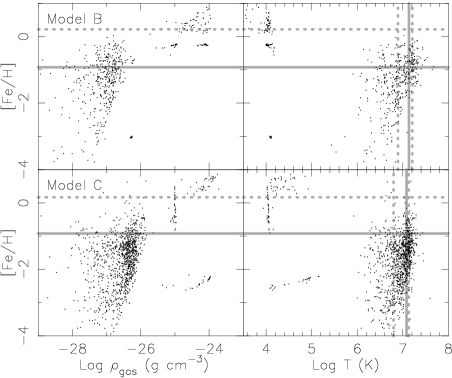
Figure 7: [Fe/H] vs density (left) and [Fe/H] vs temperature (right) distributions of gas particles within the projected radius of $R=$35 kpc for Model B (upper) and Model C (lower). The horizontal gray solid lines show [Fe/H]_X obtained by the spectrum fitting within the radius of $R=35$ kpc. The horizontal gray dotted lines correspond to mean [Fe/H] of stellar component within the radius of $R=35$ kpc. In the right panel, the vertical gray solid lines show the mean temperatures weighted by emission measure of the two temperature components (described by dotted lines) obtained by the spectrum fitting within the radius of $R=35$ kpc.

Figure 8: Comparison of the simulated CMRs (filled circle and square for Models B and C, respectively) and that of the Coma cluster ellipticals (crosses). The dashed line shows the CMR fitted to the Coma Cluster galaxies. The large (small) open circle and square demonstrate the colour and magnitude for Models B and C, when the contribution from stars whose age is younger than 2 (8) Gyr is ignored. Open star shows the position of NGC 4472.

Figure 9: Time variation of the star formation rate (upper) and the event rate of SNe II (thin lines) and SNe Ia (thick line) for Models B (left) and C (right). Solid circle (square) with error-bar in lower left (right) panel is taken from the observational SNe Ia rate by Caperrallo, Evans, & Turatto (1999). To show them clearly, those SNe Ia rates are plotted at ${\rm t}=13$ Gyr.

3.2 Optical Properties

In the last section, we showed that radiative cooling helps to explain the observed X-ray properties, such as $L_{X}$, $T_{X}$, and [Fe/H]_X. Having said that, any successful scenario must also explain the optical properties of the underlying stellar component. For this purpose, we examine the position of our simulated target galaxy in the CMR of observed elliptical galaxies. The CMR is the simple and well-studied optical scaling relation for elliptical galaxies, and gives strong constraints on the formation history of elliptical galaxies (e.g. Arimoto & Yoshii, 1987; Gibson, 1997). On the other hand, due to our self-consistent treatments of chemodynamics, the optical properties of the simulation end-products can be derived with the population synthesis as described in Section 2.3.2, and reflect the properties of stellar components, such as the age and the metallicity. Therefore, the CMR provides one of the best tests for our theoretical model of elliptical galaxies. Fig. 8 shows the comparison of the simulated galaxies with the observed Coma cluster galaxies as well as NGC 4472 in the $V-K$ and $U-V$ CMR. The data for the galaxies in the Coma cluster are from Bower, Lucey, & Ellis (1992a). Since there is no difference between S0s and ellipticals in the scaling relations which we discuss, we do not distinguish S0s from ellipticals. Bower, Lucey, & Ellis (1992a) supplies the $U-V$ and $V-K$ colours which refer to an aperture size of 11 arcsec and the $V$ band total magnitude derived from a combination of their data and the literature. We adopt the distance modulus of the Coma cluster of $m-M=34.7$ mag: the Virgo cluster distance modulus is $m-M=31.01$ (Graham et al., 1999) and the relative distance modulus of Coma with respect to Virgo is $m-M=3.69$ (Bower, Lucey, & Ellis, 1992b). This gives a luminosity distance of 87.1 Mpc for Coma. We assume that the angular diameter distance equals the luminosity distance, because the redshift of the Coma cluster ($z\sim 0.023$) is nearly zero cosmologically. Then the aperture size of 11 arcsec at the distance of the Coma cluster corresponds to $\sim$ 5 kpc. Thus, we also measure the colours within an aperture diameter of 5 kpc for the simulation end-products. The total luminosity of the simulation end-products is defined as the luminosity within the aperture radius of 50 kpc, which covers almost the whole simulated galaxy (Fig. 2).

We can see immediately that the colours of the resulting stellar components of both Models B and C are too blue and inconsistent with the observational data. This inconsistency can be traced to an excessive population of young and intermediate age stars. The strong feedback in Model C suppresses the formation of young stars, and mitigates this problem especially in the $U-V$ CMR, which is sensitive to a population of young stars. However, Model C still has too blue a colour to reproduce the observed colours. Fig. 9 shows that the histories of the star formation and SNe II and Ia rates for all the stars within $r=35$ kpc. We can see that significant amounts of stars are continuously forming until $z=0$. The SNe II and Ia rates are also too high. Caperrallo, Evans, & Turatto (1999) provide the observed SNe II and Ia rates of nearby elliptical galaxies. Their SNe II rate gives the upper limit of $0.02\times({\rm H_{0}}/75)^{2}$ SNu, and the rate of SNe Ia which they estimated is $(0.018\pm 0.06)\times({\rm H_{0}}/75)^{2}$ SNu. Here, ${\rm H_{0}}$ is the Hubble constant ( ${\rm H_{0}}=70{\rm kms^{-1}Mpc^{-1}}$ is assumed in this paper) and SNu is the number of SNe per 100 yr and $10^{10}{L}_{B,\sun}$, i.e. ${\rm SNu}=SN(100{\rm yr})^{-1}(10^{10}{L}_{B,\sun})^{-1}$. In our models, the SNe II rate is significantly higher than SNe Ia rate, which obviously contradicts this observation. In Fig. 9 symbols with error-bars show the SNe Ia rates of Caperrallo, Evans, & Turatto (1999), which is transfered from units of SNu to units used in Fig. 9 based on the $B$ band luminosity for each model. Since the luminosities of both models are too bright, compared with the observed elliptical galaxies (Fig. 8), these rates overestimate the observational data. Nevertheless, both Models B and C obviously have too many SNe Ia.

We also tried to fit the surface brightness profile by the Sersic law (see eq. 11 of Kawata, 2001b). However, we could not obtain any acceptable fit, because the stellar component is much too centrally concentrated. Such a central concentration of stars is also induced by radiative cooling which leads to continuous star formation in the high density central region. Instead, we measured the half-light radius as a radius where half the total luminosity is contained, when the total luminosity is defined as the luminosity within the aperture diameter of 100 kpc. Then, we get $V$ band half-light radii of 4.2 and 3.4 kpc for Models B and C, respectively. These are too small to reproduce the observed Kormendy relation, the relation between the half-light radius and the luminosity. Therefore, our models reproduce neither the surface brightness profile nor the size of observed elliptical galaxies, owing to excessive central radiative cooling.

Therefore, we conclude that although radiative cooling helps to explain the observed X-ray luminosity, temperature, and metallicity of elliptical galaxies, the resulting cooled gas also leads to the unavoidable overproduction of young and intermediate age stellar populations, at odds with the observational constraints. Hence, the test for both X-ray and optical properties gives stronger constraints on the theoretical model. We claim that radiative cooling alone cannot explain both X-ray and optical properties, but another physical process to suppress the recent star formation induced by cooling is required.

We found that even our extremely strong feedback assumed in Model C cannot stop radiative cooling which leads to the successive star formation. We compared the X-ray luminosity with the energy emitted by SNe II and SNe Ia in Model C, within $r=35$ kpc at z=0. The X-ray luminosity in the 0.5–10 keV pass band is $3.3\times 10^{41}$ erg s^-1. The energy emitted from SNe is estimated using the mean SNe rate for the last 1 Gyr, and provides $4.4\times 10^{43}$ erg s^-1. The energy of SNe seems larger than the X-ray luminosity. However, this X-ray luminosity is the luminosity in the 0.5–10 keV pass band. We measured the X-ray luminosity in the 0.1eV and 1 MeV pass band, and obtained $2.0\times 10^{45}$ erg s^-1. This is consistent with the total cooling rate, $1.1\times 10^{45}$ erg s^-1, of the gas particles within $r=35$ kpc, which is calculated with the cooling rate used in our simulation code. Hence, the total cooling rate is much higher than the SNe feedback energy. Model C has a higher SNe rate than the observed elliptical galaxies (Fig. 9), and the X-ray luminosity of Model C is consistent with the observation (Fig. 4). Thus, this result means that in the real elliptical galaxies SNe Ia do not generate enough energy to stop cooling.

As expected, if the contribution of the young stars was ignored, the resulting colours match the observed CMR. Open circles and squares in Fig. 8 demonstrate that if the star formation in the last 2 Gyr did not occur, the CMR of both models would become close to observational data. If the stars formed in the last 8 Gyr did not exist, the observed CMR would be roughly recovered by the increase in the colour and the decrease in the luminosity. Therefore, one exotic solution is to “hide” these younger stars within a bottom-heavy initial mass function (IMF) such that they cannot be seen today even if they did exist (e.g. Fabian, Nulsen, & Caizares, 1982; Mathews & Brighenti, 1999).

Another (more plausible) possibility is that extra heating sources, such as intermittent active galactic nuclei (AGN) activity, suppress star formation at low redshift. Before suggesting this is the true solution though, we must re-examine the predicted X-ray properties of the simulation end-products after introducing these additional heating sources; we will be pursuing this comparison in a future paper.

Figure 10: Radial dependences of $T_{X}$ and [Fe/H]_X for Models B (left panels) and C (right panels). Different symbols correspond to the values derived by the different methods, such as spectrum fitting (circles), X-ray luminosity (0.5$-$4 keV) weighted mean values (diamonds), $\rho^{2}T^{1/2}$ weighted mean values for the gas with $T>12000$ K (triangles), and $\rho^{2}T^{1/2}$ weighted mean values for the gas with $T>10^{6}$ K (stars). In the upper panels, the error-bars show the two temperatures used in fitting the X-ray spectrum, and circles indicate the mean temperatures weighted by the emission measure of the two components. The horizontal error-bars show the radius range, and the vertical error-bars indicate the 90 % confidence range obtained by the spectrum fitting.

3.3 Radial Dependences of X-ray Properties

In Section 3.1, we focused on the mean properties in the central region. In this section, we discuss X-ray properties at different radii. First, we briefly mention the dependence of the results on the analysis method. Fig. 10 shows the projected radial dependences of $T_{X}$ and [Fe/H]_X obtained by the following four different methods. Method 1 is spectrum fitting (plotted by circles and error-bars ), which is used in Section 3.1; method 2 takes the mean values weighted by the X-ray luminosity predicted by vmekal in the $0.5-4$ keV energy range (diamonds); method 3 takes the mean values weighted by $\rho^{2}T^{1/2}$ for the gas with $T>12000$ K (triangles); method 4 is the same as method 3 but only for the gas with $T>10^{6}$ K (stars). We can see that the spectrum fitting gives remarkably similar temperatures and abundances to method 4. Therefore, the results derived by the X-ray spectrum fitting reflect the properties of the high temperatures ($T>\sim 10^{6}$ K) gas. This is due to the X-ray pass band which is applied in fitting the spectrum (in this paper, 0.5$-$4 keV, which is a typical range used in the observational studies). As shown in Fig. 1 of Mathiesen & Evrard (2001), the shape of the spectrum depends on the temperature of the X-ray emitting hot gas. As a result, the gas with $T<\sim 10^{6}$ K hardly contributes to the X-ray spectrum at energies higher than 0.5 keV. For the same reason, method 3 provides different values from the ones obtained by method 1. In particular, the temperature of the central region is well bellow the ones obtained by method 1, due to the overestimate of the contribution from the low temperature ($T<\sim 10^{6}$ K) gas. Thus, if the simple $\rho^{2}T^{1/2}$ weighted mean value is used to compare the simulation results with the X-ray observational data, the temperature limit for the X-ray emitting hot gas is crucial, and should be set a temperature as high as $T=10^{6}$ K.

Except in method 3, the temperature gradient has negative slope. This is inconsistent with the observed temperature gradients in elliptical galaxies, which has a positive gradient especially at small radii (e.g. Finoguenov & Jones, 2000). The observed positive gradient in temperature is considered to be evidence for a cooling flow. On the other hand, since the ${\rm t_{cool}}={\rm t_{H}}$ line has positive slope in the density vs. temperature diagram (the right panels of Fig. 5), including radiative cooling leads to a negative temperature gradient, if the gas density profile also has a negative gradient, which is naturally expected. Thus, to explain the observed positive temperature gradient, i.e. the low temperature ($T<\sim 1$ keV) in the central region, significant amounts of the gas has to stay in the region of ${\rm t_{cool}}<{\rm t_{H}}$ in the density vs. temperature diagram for a long time, $\sim{\rm t_{H}}$. One possible physical process to realise this condition is again heating sources to balance radiative cooling, although it requires a fine-tuned physical process. In fact, the stronger feedback in Model C leads to the shallower temperature gradient than Model B (see also Fig. 5), although Model C still fails to reproduce the positive gradient.

In [Fe/H]_X, irrespective of the method, there is a clear negative gradient, which is consistent with the observational trends of some bright elliptical galaxies (e.g. Finoguenov & Jones, 2000). This is because stars, which are the source of the iron, stay within the central region corresponding to the inner most bin. This explains why the smaller aperture gives a higher [Fe/H]_X in Fig. 6.

In [Fe/H]_X, method 1 gives similar results to method 4. Particularly in the central bin, method 3 gives a higher metallicity than method 1, due to the contribution from the cooler ($T<10^{6}$ K) gas which is in the central region (Fig. 5) and enriched by stars preferentially. Surprisingly, method 2 gives higher metallicity than method 1. We found that this is because the amount of line emission increases with metallicity, and method 2 is biased towards higher metallicity gas. In fact, if the continuum X-ray luminosity is used, and line emissions are ignored, the luminosity weighted mean values agree with the values obtained by the spectrum fitting. Therefore, we should be careful when we compare the results of theoretical models with the X-ray observations.

Top panels in Fig. 11 show the 0.5–4 keV X-ray luminosity profile. We fit these profiles with the follwoing $\beta$ model, which is used to fit the observed X-ray luminosity profiles (e.g. Forman, Jones, & Tucker, 1985; Matsushita, 1997; Matsushita et al., 1998),

$$\Sigma_{X}(R)=\Sigma_{X,0}\left[1+(R/R_{\rm core})^{2}\right]^{-3\beta+0.5}.$$ (3)

In fitting, we used the data at radii less than 100 kpc, because the X-ray luminosity drops rapidly at radii further than 100 kpc. Thin lines in Fig. 11 show the best fit profile, and the parameters are summarised in Table 4. The X-ray luminosity profiles for all the Models are well described with the $\beta$ model. The typical values in the observed elliptical galaxies are $\beta\sim 0.5$ and $R_{\rm core}\sim 1$ kpc (Forman, Jones, & Tucker, 1985; Matsushita, 1997). The values of $\beta$ obtained for our models are similar to the observed values. It is worth noting that the profile for Model A is significantly steeper than those of Models B and C. Thus, radiative cooling leads to a shallower X-ray luminosity profiles, i.e., lower $\beta$. This is also a consequence of the decrease in the central hot gas density with radiative cooling (Fig. 5). On the other hand, the core radius is too large to reproduce those for the observed elliptical galaxies, irrespective of models. This is also a problem to solve for the current numerical simulation model. In model A, the core comes from the central region where the density profile is flat due to the thermal pressure of the adiabatic gas (Fig. 5). On the other hand, in Models B and C, the large core radii might be caused by a poor resolution of the simulation, because in the central region the number of the hot gas is small due to radiative cooling.

The X-ray luminosity profile is used to estimate the total mass, ${\rm M_{tot}}(r)$, within a three-dimensional radius, $r$, combined with the temperature and metallicity profiles (e.g. Forman, Jones, & Tucker, 1985; Matsushita et al., 1998). Assuming that the X-ray emitting hot gas is in a hydrostatic equilibrium and has a spherically symmetric distribution, ${\rm M_{tot,hyd}}(r)$ is written by

$${\rm M_{tot,hyd}}(r)=-\frac{kT_{\rm g}(r)r}{G\mu m_{p}}\left(\frac{d\ln\rho_{\rm g}(r)}{d\ln r}+\frac{d\ln T_{\rm g}(r)}{d\ln r}\right),$$ (4)

where $G$, $m_{p}$, and $k$ are respectively the constant of gravitation, the proton mass, and the Boltzman constant; $T_{\rm g}$ and $\rho_{\rm g}$ are the temperature and density of the X-ray emitting hot gas; $\mu=0.6$ is the mean molecular weight of the gas. Since it is easy to analyse ${\rm M_{tot}}(r)$ from the output of numerical simulations, it is interesting to compare the mass profile which is derived using equation (4), ${\rm M_{tot,hyd}}(r)$, with that derived from the simulation outputs directly, i.e. the summation of the mass of particles within the radius, ${\rm M_{tot,sum}}(r)$. To use equation (4), we need the hot gas density and temperature profile. We derived the hot gas density using the relation of

$$\rho_{\rm g}(r)=[\epsilon_{X}(r)/l_{\rm mekal}(T(r),Z(r))]^{1/2}.$$ (5)

Here, $\epsilon_{X}$ is the X-ray emission per volume, which is calculated from the following Abel integration (e.g. Binney & Merrifield, 1998) of the surface luminosity profile, $\Sigma_{X}(R)$, of equation (3),

$$\epsilon_{X}(r)=-\frac{1}{\pi}\int_{r}^{\infty}\frac{d\Sigma_{X}(R)}{dR}\frac{dR}{\sqrt{R^{2}-r^{2}}}.$$ (6)

We numerically integrate this equation and obtain $\epsilon_{X}(r)$. The expected X-ray emission, $l_{\rm mekal}$ (T,Z), is a function of temperature and metallicity, and calculated from the XSPEC vmekal model in the same X-ray pass band as $\Sigma_{X}$ (0.5–4 keV). Here, we use the metallicity, Z, which is not [Fe/H], but the total abundance of heavy elements, and assume the meteoric solar abundance pattern. Next, the three dimensional temperature and metallicity profiles are required. In observational studies, the three dimensional temperature and metallicity profiles are often assumed to equal the projected two dimensional profiles. Recently, the deprojected three dimensional profiles are also derived, assuming a spherical symmetry, and used to estimate ${\rm M_{tot,hyd}}(r)$ (e.g. Matsushita et al., 2002). Therefore, we consider the two cases of the projected profile and that derived from the three dimensional distribution of particles (deprojected profile). The thick lines in the panels of the second and third rows of Fig. 11 show the temperature and metallicity profiles of the X-ray emitting hot gas for all the models. Here, we use method 4 to derive the profiles, because methods 1 and 4 give similar X-ray observed values, as shown above. Both temperature and metallicity profiles are fitted with a power-law function, which is written by $T_{\rm g}(R)=T_{\rm g,0}[1+(R/R_{T})]^{\alpha_{T}}$ in the case of the projected temperature profile (e.g. Forman, Jones, & Tucker, 1985). The best fit profiles are presented as thin lines in Fig. 11 and the parameters are summarised in Table 4. In fitting, we used the data at radii less than 100 kpc, which is the same range as that used in fitting of the luminosity profiles. Only for the deprojected temperature profiles of Model C, we exclude the inner most bin whose value is obviously inconsistent with the assumed profile. In Model A, the metallicity is set to be zero. The fitting of the metallicity profiles in Models B and C is poor, because the profiles are not smooth. However, the metallicity profiles are less sensitive to ${\rm M_{tot,hyd}}(r)$. Finally, the bottom panels of Fig. 11 shows the derived ${\rm M_{tot,hyd}}(r)$ as well as ${\rm M_{tot,sum}}(r)$ which is the summation of the mass of all the components, i.e. DM, gas, and stars, within the three dimensional radius, $r$, in the simulation end-products. In Model A, ${\rm M_{tot,hyd}}(r)$ is consistent with ${\rm M_{tot,sum}}(r)$, which is because the X-ray emitting hot gas in Model A is in a hydrostatic equilibrium. In Models B and C, around the radius of 50 kpc, ${\rm M_{tot,hyd}}(r)$ matches with ${\rm M_{tot,sum}}(r)$. It means that even if radiative cooling is included, the status of the X-ray emitting hot gas is close to a hydrostatic equilibrium in this region. It is not surprising that ${\rm M_{tot,hyd}}(r)$ does not reproduce ${\rm M_{tot,sun}}(r)$ at larger radii ($r>100$ kpc), because we exclude those data in fitting. On the other hand, at small radii ${\rm M_{tot,hyd}}(r)$ is systematically smaller than ${\rm M_{tot,sum}}(r)$, because the hot gas is not in a hydrostatic equilibrium in this region, due to radiative cooling which continuously converts the hot gas to the cold gas. Since our simulations do not reproduce all the observed properties, we cannot judge whether or not this happens in the mass estimation from the observational data. It is also worth noting that ${\rm M_{tot,hyd}}(r)$ from the deprojected profiles (dashed lines in Fig. 11) gives higher mass and reproduces ${\rm M_{tot,sum}}(r)$ better than ${\rm M_{tot,hyd}}(r)$ from the projected profiles (solid lines in Fig. 11) in Models B and C. This is because the projected temperature underestimates the deprojected temperature, when there is a significant temperature gradient (Fig. 11). Since the temperature is constant independent of radius, in Model A, the projected temperature profile is consistent with the deprojected temperature profile,

Figure 11: Top row: the 0.5–4 keV X-ray radial luminosity profiles (thick lines) and the best-fit beta profile (thin lines). 2nd row: projected (solid lines) and deprojected (dashed lines) temperature profiles (thick lines) and the best fit profiles (thin lines). 3rd row: the projected (solid lines) and deprojected (dashed lines) metallicity profiles (thick lines) and the best fit profiles (thin lines). Bottom row: ${\rm M_{tot,sum}}(r)$ (thick lines) and ${\rm M_{tot,hyd}}(r)$ (thin lines). The solid and dashed lines corresponds to the profiles calculated from projected and deprojected temperature and metallicity profiles, respectively. In model A, the solid and dashed lines are almost overlapped, because they provides similar values.

Table 4: The results of the fitting of the luminosity, temperature, and metallicity profiles. The values in round brackets denote the results of the fitting of the deprojected profiles.

	$\log S_{0}$	$\beta$	$R_{\rm core}$	$\log T_{X,0}$	$\alpha_{T}$	$R_{\rm T}(r_{\rm T})$	$\log Z_{0}$	$\alpha_{Z}$	$R_{\rm Z}(r_{\rm Z})$
Name	(erg s-1 pc-2)		(kpc)	(keV)		(kpc)	($Z_{\sun}$)		(kpc)
A	33.6	0.86	23.8	$-$0.331 ($-$0.328)	0.15 (0.15)	128 (141)	–	–	–
B	31.5	0.35	16.8	0.250 (0.327)	0.63 (0.88)	26.8 (47.2)	$-$1.14 ($-$1.07)	0.67 (1.80)	26.2 (98.7)
C	32.5	0.51	20.4	0.097 (0.270)	3.88 (0.88)	399 (39.9)	$-$0.38 (0.19)	0.83 (0.98)	2.36 (1.32)

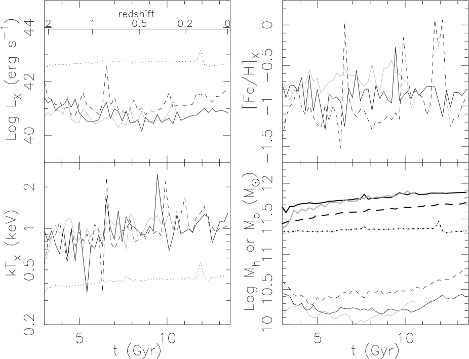
Figure 12: Time variation of the X-ray luminosity (upper left), temperature (lower left), iron abundance (upper right), and the hot (thin lines) and baryon (thick line) mass (lower right) within $R=35$ kpc. The values obtained in Model A/B/C are presented as dotted/solid/dashed lines. In the lower right panel, since in Model A almost all the baryon component within this aperture is the hot gas, the thick line overlap with the thin line. The gray line shows the results of a higher resolution simulation with the same cooling and feedback model as Model B.

3.4 Time Variation of X-ray Properties

In this paper, we focus on the properties of the simulated galaxies at $z=0$. The advantage of numerical simulation is to be able to study the evolution of galaxies, while observational data provide a snapshot of galaxies. Here, we briefly discuss the evolution history of the simulation end-products. Fig. 12 shows the X-ray properties and the hot gas and baryon mass of the simulated galaxies within $R=35$ kpc as a function of time. The X-ray luminosities are measured in the 0.5–10 keV pass band, and temperatures and iron abundances are measured by method 4 in Section 3.3. Since the number of output files in the simulations are limited, the lines are not smooth. In the X-ray luminosity, all the models have the relatively constant evolution, except for temporary increases. These temporary features are associated with the accretion of small bound objects, i.e., minor mergers. In fact, we confirmed that a small bound object passed through the central region of the target galaxy, and the gas of the objects is striped, when the X-ray luminosity increases temporarily in Model A. It is also seen in Fig. 12 that at that time the baryon and hot gas mass increases, and the temperature also increases. Although the X-ray luminosities in Models B and C are not smooth, the X-ray luminosity is always higher in the order of Models A, C, and B, as seen in Section 3.1.1. On the other hand, there is significant fluctuation in the temperatures for Models B and C, and a trend seen in Section 3.1.1, i.e. Model B has a higher temperature than Model A, represents a condition in the last 1 Gyr, when the systems are relatively stable. The mean trend of the iron abundance is constant. However, the iron abundance also changes, and gets higher values at the same time as the temperature. We consider that this is due to the SNe feedback followed by the minor mergers, which heats and enriches the gas. The baryon mass within this aperture increases continuously in Models B and C, because the gas turns into stars and the fresh gas accretes from the outer region. Since the hot high pressure gas stays in Model A, the baryon mass is relatively constant.

The numerical resolution is always a serious issue for the galaxy formation simulation, although we have achieved a high resolution at a similar level to the recent other cosmological simulations which include cooling and star formation and follow the evolution until $z=0$ (e.g. Meza et al., 2003). Since we focus on the mean properties in the scale larger than our spatial resolution, we believe that our conclusion is not heavily affected by the resolution. To examine this, we carried out a $\sim 3.375$ times (by mass) higher resolution simulation with the same parameters as Model B. In an initial condition for the higher resolution model, we have assigned high-resolution particles only in the region surrounding the target galaxies (roughly within the radius of $4\times r_{\rm vir}$ at z$=0$), to reduce the computational time. Therefore, the random seed for the small density perturbation is different from Model B, which leads to a different history of minor mergers. The mass and softening length of each gas (DM) particle in the high-resolution region are $1.74\times 10^{7}$ ($1.17\times 10^{8}$) M_☉ and 1.51 (2.86) kpc, respectively. We stop the simulation at $z\sim 0.25$, when low-resolution particles enter the virial radius of the target galaxy. The gray lines in Fig. 12 show the evolution of the X-ray properties and the hot gas and baryon mass of the simulated galaxies within $R=35$ kpc for the high-resolution model. Although detailed features are different, the mean values are roughly consistent with those of Model B. Hence, we conclude that the results presented in this paper are not sensitive to the numerical resolution. However, even in this high-resolution model the resolution is still much larger than the scales of the various physical processes, such as the star formation and the SNe feedback. The effect of such small scale physics on the large scale properties is little known, and it depends on how to model those processes. Therefore, the results shown in this paper might be affected by the modeling we adopt. Needless to say, this modeling of the small scale physics is the most crucial issue for studies of galaxy formation, which requires further investigations.

3.5 Abundance Ratios of the X-ray Emitting Hot Gas

Since we follow the evolution of the abundances of various heavy elements, we can analyse the abundance ratios of different elements. Especially, the ratios of $\alpha$ elements and Fe provide useful information about the chemical enrich history, because $\alpha$ elements, such as O and Si, are mainly produced by SNe II, while Fe is mainly produced by SNe Ia. Table 5 shows the abundance ratio of O and Si with respect to Fe (O/Fe and Si/Fe) for the X-ray emitting hot gas, the cold gas, and the stellar component within the radius of $R=$35 kpc. For the hot gas, the values obtained by method 1 and method 4 are shown. For the cold gas and stars, the mean values weighted by the mass are presented. We found that Si/H and O/H measured by method 1 are a little different from the values measured by method 4, which causes differences in O/Fe and Si/Fe between methods 1 and 4. We consider that this is because of a difficulty of the X-ray spectrum fitting due to line blending. Nevertheless, both methods give less than solar O/Fe and Si/Fe. This is consistent with the recent XMM-Newton RGS observations of O/Fe and Si/Fe in the central region of elliptical galaxies (e.g. O/Fe$=$0.4 solar in NGC 4636, O/Fe$=$0.37 and Si/Fe$=$1.04 solar in NGC 5044; Xu et al., 2002; Tamura et al., 2003). Table 6 shows the mass fraction of Fe, O, and Si ejected from SNe II, SNe Ia, and the IM stars within the last 1 Gyr for Models B and C at $R<35$ kpc. Table 6 also presents O/Fe and Si/Fe of the total ejected gas. It appears that SNe Ia are a dominant source of Fe, which induces the low O/Fe and Si/Fe. Higher Si/Fe than O/Fe is also explained by a significant contribution of SNe Ia which produce a fair amount of Si, compared to O. However, note that the rates of SNe II and SNe Ia are too high in both Models B and C, as discussed in Section 3.2 (Fig. 9). Especially, the SNe II rates in the observed elliptical galaxies are very small, and thus our high SNe II rate overestimates O and Si production. In addition, Table 5 shows that O/Fe and Si/Fe for the stellar component are solar or less, while the observed bright elliptical galaxies have over solar abundance ratios ($\alpha$/Fe$\sim$2). This is also because stars continuously form from the cold gas which has low O/Fe and Si/Fe (Table 5). This low $\alpha$/Fe for the stellar component underestimates O/Fe and Si/Fe for the mass-loss from the IM stars, although the contribution of the mass-loss of IM stars to the metal enrichment is small, compared with SNe. Hence, strictly speaking, the chemical enrichment history of our simulation is inconsistent with the observation. Nonetheless, broadly speaking, our simulation demonstrates that the observed low Si/Fe and O/Fe in the hot ISM of elliptical galaxies are explained by the dominant contribution of SNe Ia to the chemical enrichment of the X-ray emitting hot gas.

Table 5: Oxygen and Silicate abundances with respect to iron for X-ray emitting hot gas, cold gas, and stellar component at $R<$35 kpc.

	hot gas				cold gas		stars
	method 1		method 4		(T$<10^{6}$ K)
	O/Fe	Si/Fe	O/Fe	Si/Fe	O/Fe	Si/Fe	O/Fe	Si/Fe
Name	(solar)	(solar)	(solar)	(solar)	(solar)	(solar)	(solar)	(solar)
B	0.21	0.22	0.20	0.51	0.63	0.91	1.02	1.13
C	0.91	0.64	0.60	0.82	0.51	0.80	0.89	1.07

Table 6: Ejected heavy element mass fraction from SNe II, SNe Ia, and IM stars and the abundance ratios of the total ejected gas. The values denote a mean values within the last 1 Gyr from $z=0$ at $R<35$ kpc.

	SNe II			SNe Ia			IM stars			total
	fej,Fe	fej,O	fej,Si	fej,Fe	fej,O	fej,Si	fej,Fe	fej,O	fej,Si	O/Fe	Si/Fe
B	0.29	0.74	0.52	0.50	0.02	0.25	0.21	0.24	0.23	0.62	0.90
C	0.19	0.62	0.40	0.63	0.04	0.36	0.19	0.34	0.24	0.48	0.77

4 Discussion and Conclusions

Our cosmological chemodynamical simulations make it possible to undertake quantitative comparisons between the theoretical models and the observational data in both the X-ray and optical regime with minimal assumptions. This is the first attempt to explain both the X-ray and optical properties of observed elliptical galaxies by self-consistent cosmological simulations. First, we found that radiative cooling is required to explain the observed X-ray luminosity, temperature, and metallicity of elliptical galaxies. Comparison between models ignoring and including radiative cooling clarifies that radiative cooling ensures that the hot dense gas turns into the cold (i.e. non X-ray emitting) gas, and keeps X-ray emitting gas at high temperature and low density (Fig. 5). As a result, including radiative cooling leads to lower X-ray luminosity and higher X-ray weighted temperature, and provides a better agreement with the observed ${L_{X}-T_{X}}$ relation (Fig. 4). Although this effect of cooling has already been shown by previous studies (e.g. Pearce et al., 2000; Muanwong et al., 2002; Davé, Katz, & Weinberg, 2002), our study newly confirms that radiative cooling works in the same way on galactic scales using simulations with higher physical resolution. In addition, we find that stronger SNe feedback leads to higher X-ray luminosity and lower temperature, because heating by the SNe feedback makes the cooling time of the hot gas longer, and thus the gas with higher density and lower temperature is allowed to stay as X-ray emitting hot gas (Fig. 5). Radiative cooling also ensures that the hot gaseous halo has not been enriched efficiently. Stars preferentially enrich the gas in the central region, where cooling is efficient. The enriched gas can then cool easily and be incorporated into future generation of stars. In fact, we found that a large fraction of iron ejected from stars is locked into stars. This effect of cooling has been already suggested by Fujita, Fukumoto, & Okoshi (1996, 1997), although they did not consider any star formation induced by the cooled gas. Our more self-consistent numerical simulation confirms their scenario.

To summarise the X-ray study, our radiative cooling models succeed in reproducing the X-ray luminosity, temperature, and metallicity of observed elliptical galaxies. However, we also found that the resulting cooled gas leads to unavoidable overproduction of young and intermediate age stellar populations, at odds with the optical observational constraints. We examined the position of our simulated galaxy in the observed Coma cluster CMR, and found that the colours of the resulting stellar components are inconsistent with the observational data (being too blue, Fig. 8). Therefore, this study demonstrates that the cross check over both X-ray and optical properties gives stronger constraints on the theoretical models, and is essential for any successful scenario of elliptical galaxy formation and evolution. For example, our results throw doubt on the recent claim that only radiative cooling is required to explain steeper slope of the ${L_{X}-T_{X}}$ relations of groups and elliptical galaxies.

Consequently, our model fails to reproduce both X-ray and optical properties of the observed elliptical galaxies. Nevertheless, our study provides some hints to explain those observed properties. The biggest problem of the present model is too many recent (z$<$1) star formation (Fig. 8). Therefore, one exotic (if somewhat ad hoc) solution is to “hide” these younger stars within a bottom-heavy initial mass function (IMF) such that they cannot be seen today even if they did exist (e.g. Fabian, Nulsen, & Caizares, 1982; Mathews & Brighenti, 1999). A more plausible possibility is additional physical process which suppresses the cooling and star formation after the system has formed. Although we assume the extremely strong SNe feedback in Model C, it is not enough to suppress the star formation . Hence, the SNe Ia feedback is unlikely to be a candidate of this physical process, although it should contribute in some degree. We expect that extra heating by intermittent AGN activity, which is not included in our numerical model, is a major mechanism to suppress the star formation at low redshift (Brighenti & Mathews, 2002; Brüggen & Kaiser, 2002). Recent observations suggest that all elliptical galaxies have a central black hole. Therefore, once the cold gas falls into the central part of galaxy, the AGN is expected to be active and heat up the surrounding gas, and might be able to blow out the gas from the system via a radio jet. Once the gas accretion is stopped by AGN heating, the AGN itself loses fuel and goes back to a quiescent state, which allows the gas to cool again. This self-regulation cycle might be able to suppress the star formation significantly for a long time. In fact, recent high resolution X-ray images taken by Chandra reveal that the central hot gas in elliptical galaxies is not smoothly distributed, but is cavitated on scales comparable to the radio emission (e.g. Böhringer et al., 1993; Finoguenov & Jones, 2001; Jones et al., 2002). The X-ray holes are also seen on the galaxy clusters scale ($<50$ kpc), and are often coincident with extended radio lobes (e.g. McNamara et al., 2000; Allen et al., 2001; Blanton et al., 2001; Heintz et al., 2002). Those features are considered to be a relic of the significant influences of AGN activity on the hot gas of elliptical galaxies and intra cluster medium (Churazov et al., 2001).

This AGN heating mechanism might also help to solve the problem in the observed [Mg/Fe]–magnitude relation of elliptical galaxies (e.g. Matteucci, 1994; Matteucci, Ponzone, & Gibson, 1998; Kawata & Gibson, 2003). To explain the [Mg/Fe]–magnitude relation, larger galaxies are required to stop star formation at an earlier epoch. Since the recent observations claim that the black hole mass increases with the velocity dispersions of their host bulges (e.g. Merritt & Ferrarese, 2001, and reference therein), the heating effect by AGN is expected to increase with the stellar mass of elliptical galaxies, and star formation in the larger galaxies are suppressed more strongly once the AGN acts. We are planing to construct self-consistent models of this mechanism, and examine how such a self-regulation mechanism induced by AGN affects the X-ray and optical properties for elliptical galaxies with different luminosities.

References

- Aaronson, Persson, & Frogel (1981) Aaronson M., Persson S.E., Frogel J.A., 1981, ApJ, 245, 18
- Allen et al. (2001) Allen S.W., Taylor G.B., Nulsen P.E.J. et al., 2001, MNRAS, 324, 842
- Anders & Grevesse (1989) Anders E., Grevesse N., 1989, Geochim. Cosmochim. Acta, 53, 197
- Arimoto & Yoshii (1987) Arimoto N., Yoshii Y., 1987, A&A, 173, 23
- Arimoto et al. (1997) Arimoto N., Matsushita K., Ishimaru Y., Ohashi T., Renzini A., ApJ, 477, 128
- Awaki et al. (1994) Awaki H., Mushotzky R., Tsuru T. et al., 1994, PASJ, 46, L65
- Barnes & Hut (1986) Barnes J.E., Hut P., 1986, Nature, 324, 446
- Bekki (1998) Bekki K., 1998, ApJ, 504, 50
- Bertschinger (2001) Bertschinger E., 2002, ApJS, 137, 1
- Binney & Merrifield (1998) Binney J., Merrifield M., 1998, Galactic Astronomy. Princeton Univ. Press, Princeton
- Blanton et al. (2001) Blanton E.L., Sarazin C.L., McNamaraB.R., Wise M.W., 2001, ApJL, 558, L15
- Bower et al. (2001) Bower R.G., Benson A.J., Lacey C.G., Baugh C.M., Cole S., Frenk C.S., 2001, MNRAS, 325, 497
- Bower, Lucey, & Ellis (1992a) Bower R.G., Lucey J.R., Ellis R.S., 1992a, MNRAS, 254, 589
- Bower, Lucey, & Ellis (1992b) Bower R.G., Lucey J.R., Ellis R.S., 1992b, MNRAS, 254, 601
- Böhringer et al. (1993) Böhringer H., Voges W., Fabian A.C., Edge A.C., Neumann D.M., 1993, MNRAS, 264, L25
- Bregman, Hogg, & Roberts (1992) Bregman J.N., Hogg D.E., Roberts M.S., 1992, ApJ, 387, 484
- Brighenti & Mathews (1999) Brighenti F., Matthews W.G., 1999, ApJ, 515, 542
- Brighenti & Mathews (2002) Brighenti F., Matthews W.G., 2002, ApJL, 574L, 11
- Brüggen & Kaiser (2002) Brüggen M., Kaiser C.R., 2002, Nature, 418, 301
- Bryan (2000) Bryan G.L., 2000, ApJL, 544, 1
- Buote (1999) Buote D.A., MNRAS, 309, 685
- Buote (2002) Buote D.A., ApJL, 574, 135
- Buote & Fabian (1998) Buote D.A., Fabian A.C., MNRAS, 296, 977
- Buote et al. (2003) Buote D.A., Lewis A.D., Brighenti F., Mathews W.G., ApJ in press (astro-ph/0205362)
- Caperrallo, Evans, & Turatto (1999) Cappellaro E., Evans R., Turatto M., 1999, A&A, 351, 459
- Churazov et al. (2001) Churazov E., Brüggen M., Kaiser C.R., Böhringer H., Forman W., 2001, ApJ, 554, 261
- Ciotti et al. (1991) Ciotti L., D’Ercole A., Pellengrini S., Renzini A., 1991, ApJ, 376, 380
- Davé, Katz, & Weinberg (2002) Davé R., Katz N., Weinberg D.H., 2002, ApJ, 579, 23
- Djorgovski & Davis (1987) Djorgovski S., Davis M., 1987, ApJ, 313, 59
- Dressler et al. (1987) Dressler A., Lynden-Bell D., Burstein D., Davies R.L., Faber S.M., Terlevich R.J., Wegner G., 1987, ApJ, 313, 42
- Edge (2001) Edge A.C., 2001, MNRAS, 328, 762
- Edge & Stewart (1991) Edge A.C., Stewart G.C., 1991, MNRAS, 252, 414
- Eke, Navarro, & Frenk (1998) Eke V.R., Navarro J.F., Frenk C.S., 1998, ApJ, 503, 569
- Evrard & Henry (1991) Evrard A.E., Henry J.P., 1991, ApJ, 383, 95
- Fabian, Nulsen, & Caizares (1982) Fabian A.C., Nulsen P.E.J., Canizares C.R., 1982, MNRAS, 201, 933
- Forman et al. (1979) Forman, W., Schwarz J., Jones C., Liller W., Fabian A.C., 1979, ApJL, 15, 27
- Forman, Jones, & Tucker (1985) Forman, W., Jones C., Tucker W., 1983, ApJ, 293, 102
- Finoguenov & Jones (2000) Finoguenov A., Jones C., 2000, ApJ, 539, 603
- Finoguenov & Jones (2001) Finoguenov A., Jones C., 2001, ApJL, 547, L107
- Fujita, Fukumoto, & Okoshi (1996) Fujita Y., Fukumoto J., Okoshi K., 1996, ApJ, 470, 762
- Fujita, Fukumoto, & Okoshi (1997) Fujita Y., Fukumoto J., Okoshi K., 1997, ApJ, 488, 585
- Georgakakis et al. (2001) Georgakakis A., Hopkins A.M., Caulton A., Wiklind T., Terlevich A.I., Forbes D.A., 2001, MNRAS, 326, 1431
- Gibson (1997) Gibson B.K., 1997, MNRAS, 290, 471
- Gingold & Monaghan (1977) Gingold R.A., Monaghan J.J., 1977, MNRAS, 181, 375
- Graham et al. (1999) Graham J.A., Ferrarese L., Freedman W.L., Kennicutt R.C.Jr., Mould J.R., Saha A., Stetson P.B., Madore B.F., Bresolin F., Ford H.C., Gibson B.K., Han M., Hoessel J.G., Huchra J., Hughes S.M. Illingworth G.D., Kelson D.D., Macri L., Phelps R., Sakai S., Silbermann N.A., Turner A., 1999, ApJ, 516, 626
- Hattori, Habe, & Ikeuchi (1987) Hattori M., Habe A., Ikeuchi S., 1987, Prog. Theo. Phys., 78, 1099
- Helsdon & Ponman (2000) Helsdon S.F., Ponman T.J., 2000, MNRAS, 315, 356
- Heintz et al. (2002) Heintz S., Choi Y.-Y., Reynolds C.S., Begelman M.C., 2002, ApJL, 569, L79
- Hernquist & Katz (1989) Hernquist L., Katz N., 1989, ApJS, 70, 419
- Hultman & Pharasyn (1999) Hultman J., Pharasyn A., 1999, A&A, 347, 769
- Iwamoto et al. (1999) Iwamoto K., Brachwitz F., Nomoto K., Kishimoto N., Umeda H., Hix W.R., Thielemann F.-K., 1999, ApJS, 125, 439
- Jones et al. (2002) Jones C., Forman W., Vikhlinin A., Markevitch M., David L., Warmflash A., Murray S., Nulsen P. E. J., 2002, ApJL, 567, L115
- Kaastra (1992) Kaastra J.S., 1992, An X-Ray Spectral Code for Optically Thin Plasmas (Internal SRON-Leiden Report, updated version 2.0)
- Kaiser (1991) Kaiser N., 1991, ApJ, 383, 104
- Katz, Weinberg, & Hernquist (1996) Katz N., Weinberg D.H., Hernquist L., 1996, ApJS, 105, 19
- Katz & White (1995) Katz N., White S.M.D., 1995, ApJ, 412, 455
- Kawata (1999) Kawata D., 1999, PASJ, 51, 931
- Kawata (2001a) Kawata D., 2001a, ApJ, 548, 703
- Kawata (2001b) Kawata D., 2001b, ApJ, 558, 598
- Kawata & Gibson (2003) Kawata D., Gibson B.K., MNRAS, 2003, 340, 908
- Käellander & Hultman (1998) Käellander D., Hultman J., 1998, A&A, 333, 399
- Kay et al. (2000) Kay S.T., Pearce F.R., Jenkins A., Frenk C.S., White S.D.M., Thomas P.A., Couchman H.M.P., 2000, MNRAS, 316, 374
- Kobayashi, Tsujimoto, & Nomoto (2000) Kobayashi C., Tsujimoto T., Nomoto K., 2000, ApJ, 539, 26
- Kodama (1997) Kodama T., 1997, Ph.D. thesis, University of Tokyo
- Kodama & Arimoto (1997) Kodama T., Arimoto N., 1997, A&A, 320, 41
- Lewis et al. (2000) Lewis G.F., Babul, A., Katz N., Quinn T., Hernquist L., Weinberg D.H., 2000, ApJ, 536, 623
- Liedahl Osterheld, & Goldstein (1995) Liedahl D.A., Osterheld A.L., Goldstein W.H., 1995, ApJL, 438, 115
- Lloyd-Davies, Ponman, & Cannon (2000) Lloyd-Davies E.J., Ponman T.J., Cannon D.B., 2000, MNRAS, 315, 689
- Loewenstein (2000) Loewenstein M., 2000, ApJ, 532, 17
- Loewenstein & Mathews (1991) Loewenstein M., Mathews W.G., 1991, ApJ, 373, 445
- Loewenstein et al. (1994) Loewenstein M., Mushotzky R.F., Tamura T. et al., 1994, ApJL, 436, 75
- Lucy (1977) Lucy L.B., 1977, AJ, 82, 1013
- Mathews & Brighenti (1999) Mathews W.G., Brighenti F., 1999, ApJ, 526, 114
- Mathews & Loewenstein (1986) Mathews W.G., Loewenstein M., 1996, ApJL, 306, 7
- Mathiesen & Evrard (2001) Mathiesen B.F., Evrard A.E., 2001, ApJ, 546, 100
- Matsushita (1997) Matsushita K., 1997, Ph.D. thesis, University of Tokyo
- Matsushita et al. (2002) Matsushita K., Belsole E., Finoguenov A., Böhringer H., 2002, A&A, 386, 77
- Matsushita et al. (1998) Matsushita K., Makishima K., Ikebe Y., Rokutada E., Yamasaki, N.Y., Ohashi T., 1998, ApJL, 499, L13
- Matsushita, Ohashi, & Makishima (2000) Matsushita K., Ohashi T., Makishima K., 2000, PASJ, 52, 685 (MOM00)
- McNamara et al. (2000) McNamara B.R.,, Wise M., Nulsen P.E.J. et al., 2000, ApJL, 534, L135
- Merritt & Ferrarese (2001) Merritt D., Ferrarese L., 2001, ApJ, 547, 140
- Mewe, Gronenschild, & van den Oord (1985) Mewe R., Gronenschild E.H.B.M., van den Oord G.H.J., 1985, A&AS, 62, 197
- Mewe, Lemen, & van den Oord (1986) Mewe R., Lemen J.R.., van den Oord G.H.J., 1986, A&AS, 65, 511
- Meza et al. (2003) Meza A., Navarro J.F., Steinmetz M., Eke V., 2003, ApJ, 590, 619
- Matsumoto et al. (1997) Matsumoto H., Koyama K., Awaki H., Tsuru T., Loewenstein M., Matsushita K., 1997, ApJ, 482, 133
- Matsushita, Ohashi, & Makishima (2000) Matsushita K., Ohashi T., Makishima K., 2000, PASJ, 52, 685
- Matteucci (1994) Matteucci F. 1994, A&A, 288, 57
- Matteucci, Ponzone, & Gibson (1998) Matteucci F., Ponzone R., & Gibson B.K. 1998, A&A, 335, 855
- Muanwong et al. (2001) Muanwong O., Thomas P.A., Kay S.T., Pearce F.R., Couchman H.M.P., 2001, ApJL, 552, L27
- Muanwong et al. (2002) Muanwong O., Thomas P.A., Kay S.T., Pearce F.R., 2002, MNRAS, 336, 527
- Navarro, Frenk, & White (1995) Navarro J.F., Frenk, C.S., White, S.D.M., 1995, NNRAS, 275, 720
- Navarro, Frenk, & White (1997) Navarro J.F., Frenk, C.S., White, S.D.M., 1997, ApJ, 490, 493
- Navarro & White (1993) Navarro J.F., White, S.D.M., 1993, MNRAS, 265, 271
- Padmanabhan (1993) Padmanabhan T., 1993, Structure formation in the universe. Cambridge Univ. Press, Cambridge
- Pearce et al. (2000) Pearce F.R., Thomas P.A., Couchman M.P., Edge A.C., 2000, MNRAS, 317, 1029
- Ponman, Cannon, & Navarro (1999) Ponman T.J., Cannon D.B., Navarro J.F., 1999, Nature, 397, 135
- Raymond & Smith (1977) Raymond J.C., Smith B.W., 1977, ApJS, 35, 419
- Sakelliou et al. (2002) Sakelliou I., Peterson J.R., Tamura T. et al., 2002, A&A 391, 903
- Salpeter (1955) Salpeter E.E., 1955, ApJ, 121, 161
- Sandage (1972) Sandage A., 1972, ApJ, 176, 21
- Sarazin, Irwin, & Bregman (2001) Sarazin C.L., Irwin J.A.,, Bregman J.N. 2001, ApJ, 556, 533
- Sutherland & Dopita (1993) Sutherland R.S., Dopita M.A., 1993, ApJS, 88, 253
- Springel & Hernquist (2003) Springel V., Hernquist L., 2003, MNRAS, 339, 289
- Tamura et al. (2003) Tamura T., Kaastra J.S., Makishima K., Takahashi I., 2003, A&A in press (astro-ph/0211603)
- Thacker & Couchman (2000) Thacker R.J., Couchman H.M.P., 2000, ApJ, 545, 728
- Toft et al. (2002) Toft S., Rasmussen J., Sommer-Larsen J., Pedersen K., 2002, MNRAS, 335, 799
- van den Hoek & Groenewegen (1997) van den Hoek L.B., Groenewegen M.A.T., 1997, A&AS, 123, 305
- Valdarnini (2003) Valdarnini R., 2003, MNRAS, 339, 1117
- Voit & Bryan (2001) Voit M.G., Bryan G.L., 2001, Nature, 414, 425
- Woosley & Weaver (1995) Woosley S.E., Weaver T.A., 1995, ApJS, 101, 181
- Wu, Fabian, Nulsen (2000) Wu K.K.S., Fabian A.C., Nulsen P.E.J., 2000, MNRAS, 318, 889
- Xu et al. (2002) Xu H., Kahn S.M., Peterson J.R. et al., 2002, ApJ, 579, 600
- Xue & Wu (2000) Xue Y.-J., Wu X.-P., 2000, ApJ, 538, 65
- Yepes et al. (1997) Yepes, G., Kates, R., Khokhlov, A., Klypin, A. 1997, MNRAS, 284, 235
- Yoshikawa, Jing, & Suto (2000) Yoshikawa K., Jing Y.P., Suto Y., 2000, ApJ, 535, 593