Constraints on extended quintessence from high-redshift Supernovae

Abstract

We obtain constraints on quintessence models from magnitude-redshift measurements of 176 type Ia Supernovae. The considered quintessence models are ordinary quintessence, with Ratra-Peebles and SUGRA potentials, and extended quintessence with a Ratra-Peebles potential. We compute confidence regions in the $\Omega_{m0}-\alpha$ plane and find that for SUGRA potentials it is not possible to obtain useful constraints on these parameters; for the Ratra-Peebles case, both for the extended and ordinary quintessence we find $\alpha\raise-3.0pt\hbox{\hbox to0.0pt{\hbox{\hskip 3.0pt $\sim$}\hss}\raise 4.0pt\hbox{\hskip 3.0pt$<$}\ }0.8$, at the $1\sigma$ level. We also consider simulated dataset for the SNAP satellite for the same models: again, for a SUGRA potential it will not be possible to obtain constraints on $\alpha$, while with a Ratra-Peebles potential its value will be determined with an error $\raise-3.0pt\hbox{\hbox to0.0pt{\hbox{\hskip 3.0pt $\sim$}\hss}\raise 4.0pt\hbox{\hskip 3.0pt$<$}\ }0.6$. We evaluate the inaccuracy made by approximating the time evolution of the equation of state with a linear or constant $w(z)$, instead of using its exact redshift evolution. Finally we discuss the effects of different systematic errors in the determination of quintessence parameters.

1 Introduction

Cosmological tests such as the baryon fraction in galaxy clusters (Hradecky et al. 2000; Allen et al. 2002), the abundance of massive galaxy clusters (see e.g. Bahcall 2000; Borgani et al. 2001), the magnitude-redshift relation for type Ia Supernovae (Riess et al. 1998; Perlmutter et al. 1999; Gott et al. 2001; Tonry et al. 2003), the statistical analysis of the galaxy distribution in large redshift catalogs (e.g. Percival et al. 2001; Verde et al. 2002) and Cosmic Microwave Background (CMB) anisotropies Bennett et al. (2003); Spergel et al. (2003) indicate a low value for the matter density parameter today, $\Omega_{m0}$, probably lying in the interval $0.15\raise-3.0pt\hbox{\hbox to0.0pt{\hbox{\hskip 3.0pt $\sim$}\hss}\raise 4.0pt\hbox{\hskip 3.0pt$<$}\ }\Omega_{m0}\raise-3.0pt\hbox{\hbox to0.0pt{\hbox{\hskip 3.0pt $\sim$}\hss}\raise 4.0pt\hbox{\hskip 3.0pt$<$}\ }0.4$. Recent results from the study of CMB anisotropies obtained with the WMAP satellite (Bennett et al. 2003) also provide strong support for a flat (or very nearly flat) Universe. Combining these two different indications leads to the hypothesis that a new form of energy, named dark energy (DE), fills the gap between $\Omega_{m0}$ and unity: $\Omega_{m0}+\Omega_{DE0}=1$.

One of the main goals of modern cosmology is to explain the nature of dark energy. The simplest solution to this problem is to introduce a cosmological constant $\Lambda$ in our Universe model. This scenario can have a simple theoretical interpretation, as $\Lambda$ can be related to the energy density of the vacuum state in quantum field theory (Zel’dovich 1968). Unfortunately, this simple explanation results in a very large (formally infinite) value for the vacuum energy density, which is larger by tens of orders of magnitude than the observed one (of the order of $10^{-47}$ GeV⁴). What emerges is a fine-tuning problem, namely the “cosmological constant problem”. Another apparently unnatural feature of the cosmological constant model is that it starts to dominate the Universe evolution only in the very near past. This issue is usually referred to as the “cosmic coincidence problem” and reduces to a fine-tuning problem in the choice of the initial conditions, in particular of the value of $\Lambda$.

A possible way of alleviating these problems is to allow for a time variation of the dark energy density, which is constant if due to $\Lambda$. A very interesting class of models with this property goes under the name of quintessence (Coble et al. 1997; Caldwell et al. 1998; Ferreira & Joyce 1998; Viana & Liddle 1998).

One of the most promising cosmological tests on the properties of the dark energy component is based on the already mentioned magnitude-redshift relation for type Ia Supernovae (see e.g. Brax & Martin 1999; Podariu & Ratra 2000; Podariu et al. 2001; Goliath et al. 2001; Weller & Albrecht 2001, 2002; Eriksson & Amanullah 2002; Gerke & Efstathiou 2002; Padmanabhan & Choudhury 2003; Di Pietro & Claeskens 2003; Knop et al. 2003). In fact, these objects can be considered as good standard candles, which makes it possible to determine their luminosity distance, whose dependence on redshift is specific of each particular cosmological framework.

In this paper we will focus on three different kinds of quintessence models whose features are briefly described in Section 2. In Section 3 we present the constraints obtained on these models using the magnitude-redshift relation for existing type Ia Supernovae (SNIa) data. In Section 4 we illustrate how the constraints will improve with the SuperNovae Acceleration Probe (SNAP) satellite which is currently being projected and will be devoted to the discovery and study of SNIa (Aldering et al. 2002; see also: http://snap.lbl.gov); we also check the validity of approximating the exact redshift evolution of the equation of state with a linear or constant behavior and discuss the possible effects of different systematic errors on the parameter determination. Finally, in Section 5 we present our conclusions.

2 Theoretical framework

In this paper we focus on the Extended Quintessence (EQ) models, introduced in (Perrotta et al. 1999; Baccigalupi et al. 2000). Extended quintessence and related models have been also considered in (Chiba 1999, 2001; Uzan 1999; Bartolo & Pietroni 2000; Boisseau et al. 2000; de Ritis et al. 2000; Faraoni 2000; Fujii 2000; Chen et al. 2001; Bean 2001; Gasperini 2001; Perrotta & Baccigalupi 2002; Riazuelo & Uzan 2002; Torres 2002; Kneller & Steigman 2003).

For these models the evolution of the scale factor $a$ and the scalar field $\phi$ responsible for the quintessence component can be obtained by solving the set of equations:

$${H}^{2}\equiv\left(\frac{\dot{a}}{a}\right)^{2}=\frac{1}{3F}\left(a^{2}\rho_{fluid}+\frac{1}{2}\dot{\phi}^{2}+a^{2}V-3{H}\dot{F}\right),$$ (1)

$$\ddot{\phi}+2{H}\dot{\phi}=\frac{a^{2}}{2}F_{\phi}R-a^{2}V_{\phi}\ .$$ (2)

In the previous equations the dots denote derivatives with respect to the conformal time and the subscript $\phi$ denotes differentiation with respect to the scalar field; $R$ is the Ricci scalar; $\rho_{fluid}$ represents the energy density associated with all the constituents of the Universe except for the quintessence scalar field; $V\left(\phi\right)$ is the quintessence potential and finally $F\left(\phi\right)$ is a function specifying the form of the coupling between $\phi$ and gravity. Hereafter we will always refer to the non-minimally coupled (NMC) scalar field models Perrotta et al. (1999), for which the function $F$ is defined as $F\left(\phi\right)={1}/{8\pi G}+\tilde{F}\left(\phi\right)-\tilde{F}\left(\phi_{0}\right)$, where $\tilde{F}\left(\phi\right)=\xi\phi^{2}$. This kind of models has two free parameters: the dimensionless constant $\xi$, parametrizing the amount of coupling, and the present value of the scalar field $\phi_{0}$.

The coupling between the scalar field and gravity generates a time-varying gravitational constant (see e.g. the review by Uzan 2003). Upper bounds on this variation come from local laboratory and solar system experiments Gillies (1997) and from the effects induced on photon trajectories (Reasenberg et al. 1979; Will 1984; Damour 1998). As pointed out by Perrotta et al. (2000), these bounds become constraints on the parameters of the models:

$$32\pi G\xi^{2}\phi_{0}^{2}\leq\frac{1}{500}.$$ (3)

We will use the previous inequality in the next sections in order to improve our determination of the cosmological parameters.

For completeness and in order to allow a comparison with similar analyses, we will also consider the case of ordinary quintessence (OQ), i.e. models for which there is no direct coupling between the scalar field and gravity (it is often referred to as the minimal coupling case). OQ can be easily obtained from EQ in the limit of $\xi\rightarrow 0$.

If we want to completely specify a quintessence model, we have to choose the analytical form for the potential $V\left(\phi\right)$. One of the main advantages of a time-varying dark energy density is that it is possible to alleviate the cosmic coincidence problem. This is achieved by assuming particular classes of potentials, the so-called “tracker potentials” (Steinhardt et al. 1999), for which one obtains at low redshifts the same time evolution for $a$ and $\phi$, even starting from initial conditions which differ by orders of magnitude: this leads to a dark energy dominated era close to the present time, without fine-tuning on the initial conditions. For the following analysis, we will consider two different classes of tracker potentials: the inverse power-law Ratra-Peebles potential (hereafter RP; Ratra & Peebles 1988; see also Peebles & Ratra 2003 and references therein)

$$V\left(\phi\right)=\frac{M^{4+\alpha}}{\phi^{\alpha}},$$ (4)

and the SUGRA potential (Binétruy 1999; Brax & Martin 1999):

$$V=\frac{M^{4+\alpha}}{\phi^{\alpha}}\exp{\left(4\pi G\phi^{2}\right)}.$$ (5)

In particular, we will use the potential (4) in the context of both EQ and OQ models, while the potential (5) will be considered in the minimal coupling ($\xi=0$) case, only.

We solved numerically Eqs.(1) and (2) in the tracking regime. The behaviors we found for $a(t)$ and $\phi(t)$ (not shown in figure) are in excellent agreement with those obtained by Baccigalupi et al. (2000), whose analysis also includes the Ratra-Peebles case in the framework of EQ. In the next section we will use these results to obtain our theoretical estimates of the luminosity distance $d_{L}$.

3 Constraints from present high-redshift supernovae data

The purpose of this section is to test the possibility of constraining the cosmological parameters describing quintessence models by using the best SNIa dataset presently available. To this aim we build a sample combining data coming from the literature. As a starting point, we consider the data reported in Table 15 of Tonry et al. (2003). In particular, we use for our analysis the subset which is presented by the authors as the most reliable one for cosmological studies. This data compilation, comprising 172 SNIa, is obtained by eliminating from the original whole sample of 230 SNIa the objects at low redshift ($z<0.01$) and those with high reddening ($A_{V}>0.5$ mag). Then, we consider the data from Table 3 of Knop et al. (2003), but including in the sample only SNIa belonging to their “low-extinction primary subset” (7 objects). In their Table 4, Knop et al. (2003) present the new fits to the Perlmutter et al. (1999) data, which are already included in the Tonry et al. (2003) sample. In this case we decided to use the magnitudes from Knop et al. (2003), because they are obtained using new fitting lightcurves. The two catalogues have also SNIa in common in the low-redshift sample, taken from Hamuy et al. (1996) and Riess et al. (1999). For these we prefer to use the data reported by Tonry et al. (2003) because they are obtained as a median of different fitting methods. For coherence with our previous choice, we decided to exclude 5 objects, present in the low-redshift and Perlmutter et al. (1999) samples, but excluded by the “low-extinction primary subset” of Knop et al. (2003). Finally, we add two new SNIa, 2002dc and 2002dd, recently studied by Blakeslee et al. (2003). Therefore the sample of SNIa here considered comprises 176 objects.

To constrain the cosmological parameters, we compare through a $\chi^{2}$ analysis the redshift dependence of the observational estimates of $\log{\left(d_{L}\right)}$ to their theoretical values, which for a flat, matter or dark energy dominated universe can be obtained as

$$d_{L}(z)=\frac{1+z}{H_{0}}\int_{0}^{z}{\left[\frac{\Omega_{m0}\left(1+z^{\prime}\right)^{3}+\Omega_{\phi 0}f(z^{\prime})}{8\pi GF}\right]^{-{1}/{2}}dz^{\prime}},$$ (6)

where

$$f(z)=\exp{\left(3\int_{0}^{z}{\frac{1+w(z^{\prime})}{1+z^{\prime}}dz^{\prime}}\right)}.$$ (7)

Here $H_{0}$ is the present value of the Hubble constant, and $\Omega_{m0}$ and $\Omega_{\phi 0}$ represent the contributions to the present density parameter due to matter and scalar field, respectively. The quantity $w\equiv p_{\phi}/\rho_{\phi}$ sets the equation of state relating the scalar field pressure

$$p_{\phi}=\frac{\dot{\phi}^{2}}{2a^{2}}+V(\phi)-\frac{3H\dot{F}}{a^{2}}$$ (8)

and its energy density

$$\rho_{\phi}=\frac{\dot{\phi}^{2}}{2a^{2}}-V(\phi)+\frac{\ddot{F}}{a^{2}}+\frac{H\dot{F}}{a^{2}}\ .$$ (9)

The quantity $w(z)$ can be computed by using the numerical solutions of the previous equations, once a cosmological model is assumed.

We can now find, for the different quintessence models described in the previous section, the parameters (and their confidence regions) which best fit the SNIa data by using the standard $\chi^{2}$ method. For this analysis we have to consider the errors on the distance moduli. For the objects coming from Tonry et al. (2003), they are obtained directly from their Table 15, once a value for $H_{0}$ is assumed. On the other hand, Knop et al. (2003) report errors for the apparent magnitudes of their SNIa. We obtain the uncertainty on the distance modulus by adding in quadrature an error of 0.05 in the estimate of the absolute magnitude, as suggested by the data of Hamuy et al. (1996), Riess et al. (1999) and Knop et al. (2003), Table 4. In addition, we include an extra contribution to the error coming from the possible uncertainty in the peculiar velocities. In particular, following Tonry et al. (2003) we add $500$ km s^-1 divided by the redshift in quadrature to the distance error.

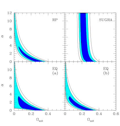
Figure 1: Confidence regions ($\Delta\chi^{2}=2.30,5.99,11.8$, corresponding to 1, 2 and 3$\sigma$ for a Gaussian distribution with two free parameters, respectively) for the parameters $\Omega_{m0}$ and $\alpha$, as obtained using the sample of 176 SNIa data presently available. Different panels refer to different quintessence models: ordinary quintessence with a Ratra-Peebles potential (top left); ordinary quintessence with a SUGRA potential (top right); extended quintessence with a Ratra-Peebles potential (bottom left); extended quintessence with a Ratra-Peebles potential when the upper limits on the time variation of the gravitational constant are satisfied (bottom right).

We compute the values for $\chi^{2}$ on a regular grid of the considered parameters ($\Omega_{m0}$, $\alpha$ and $\xi$ for the EQ models; $\Omega_{m0}$ and $\alpha$ for the OQ models), looking for its minimum value, $\chi^{2}_{\rm min}$. In particular, we allow $\Omega_{m0}$ to vary between 0 and 1 with spacing of 0.001; $\alpha$ between 0 and 12 with spacing of 0.1 and $\xi$ between 0.001 to 0.100 with spacing of 0.001. The results in the plane $\Omega_{m0}-\alpha$ are shown in Figure 1, where we display the contours of constant $\Delta\chi^{2}\equiv\chi^{2}-\chi^{2}_{\rm min}=2.30,5.99$ and 11.80, corresponding to $1\sigma$, $2\sigma$ and $3\sigma$ for a Gaussian distribution with two free parameters, respectively.

The top-left panel refers to the ordinary quintessence model with a RP potential. In this case we find $\chi^{2}_{\rm min}=206$ for $\Omega_{m0}=0.30$ and $\alpha=0.0$. However, from the plot it is evident that there is a strong degeneracy between the two free parameters $\alpha$ and $\Omega_{m0}$ and it is not possible to obtain strong constraints on them at the same time. Nevertheless, we can extract some information by considering the $\chi^{2}$ distribution when only a single parameter is allowed to vary. In this case, we obtain the errorbars associated to the best fit value by assuming $\Delta\chi^{2}=1$, which corresponds to $1\sigma$ for a Gaussian distribution with one single parameter. The SNIa dataset we used does not allow to obtain tight constraints on the parameter $\alpha$: $\alpha<0.83$ at the $1\sigma$ confidence level, with a best fit value of $\alpha=0$. In addition, we obtain $\Omega_{m0}=0.30^{+0.03}_{-0.10}$, for the matter density parameter. If we impose the Gaussian prior $\Omega_{m0}=0.27\pm 0.04$, as suggested by the combined analysis of recent CMB observations and large-scale structure data Spergel et al. (2003), we obtain $\alpha<0.47$ at the $1\sigma$ confidence level (best fit value: $\alpha=0.10$). We notice that our results are in agreement with those obtained from a similar analysis carried out by Podariu & Ratra (2000), even though, thanks to the improvement in the SNIa dataset, the confidence contours start to close off, at least at the $1\sigma$ confidence level.

In the top-right panel we report the results still for the OQ model, but with the SUGRA potential. The values for $\chi^{2}_{\rm min}$ and the corresponding parameters are the same obtained for the RP potential. In this case the confidence regions are almost vertical, showing a very small dependence on $\alpha$: this does not allow us to extract constraints on $\Omega_{m0}$ and $\alpha$. Only if we impose the Gaussian prior $\Omega_{m0}=0.27\pm 0.04$, we are able to obtain $\alpha<2.78$ at the $1\sigma$ level (best fit value: $\alpha=0.24$).

In the two bottom panels of Figure 1 we present the results for the model with EQ and a RP potential. In this case we have three free parameters: in addition to $\alpha$ and $\Omega_{m0}$, there is $\xi$, which parametrizes the strength of the coupling between the scalar field and gravity. In the bottom-left panel we show the two-dimensional confidence regions in the $\alpha-\Omega_{m0}$ plane as obtained by minimizing $\chi^{2}$ with respect to $\xi$: they appear very similar to the previous case of ordinary quintessence with RP potential, only slightly larger. Again it is convenient to discuss the results when a single free parameter is considered. Unfortunately, there are no possibilities to obtain constraints on $\xi$ (best fit for $\xi=0.001$), even at the $1\sigma$ confidence level. For the other two parameters our results are again very similar to that of ordinary quintessence with RP potential: $\alpha<0.82$ (best fit $\alpha=0.02$) and $\Omega_{m0}=0.28^{+0.05}_{-0.09}$. The bottom-right panel shows how the confidence regions change when the upper limits on the time variation of the gravitational constant are taken into account. The constraints on $\alpha$ and $\Omega_{m0}$ do not change significantly: $\alpha<0.82$ and $\Omega_{m0}=0.28^{+0.04}_{-0.09}$, respectively. Considering $\xi$, the inclusion of the upper bounds does not improve the situation, and $\xi$ remains completely undetermined.

Finally, instead of imposing the constraints just described, we can consider the prior $\Omega_{m0}=0.27\pm 0.04$. Again, we cannot obtain useful bounds on $\xi$, while we obtain $\alpha<0.45$ at the $1\sigma$ level (best fit: $\alpha=0.11$). The previous results clearly show the necessity for new samples of SNIa. The SNAP satellite will be dedicated to this purpose: in the next section we will check the improvement that it will allow on the determination of the cosmological parameters.

The results presented in this section assume that all the data points are purely governed by statistical errors. Even if we carefully selected our SNIa sample in order to reduce possible systematic errors, their importance in the present data cannot be completely excluded. As largely discussed in Knop et al. (2003, see also Tonry et al. 2003), systematics can have different origins, In particular Knop et al. (2003) studied the effects on the determination of the cosmological parameters (they considered $\Omega_{m0}$, $\Omega_{\phi 0}$, $w$) coming from different SNIa selection, lightcurve fitting methods, contamination from non-type Ia supernovae, Malmquist bias, gravitational lensing, dust properties, etc. Their conclusion is that the total systematic error is of the same order of magnitude as the statistical uncertainty. Because of the weakness of the constraints we obtained on $\alpha$ and $\xi$ using present SNIa data, we prefer to leave an extended discussion of systematics to the next section, where we will present the expected results from the SNAP satellite. However, here we report the results of some tests which have been done. In order to verify if our sample suffers from selection effects, we repeated our analysis by considering only 54 SNIa belonging to the low-extinction primary subset of Knop et al. (2003) and coming only from the Supernova Cosmology Project. Because of the smallness of this sample, the resulting constraints cannot be directly compared to those obtained from the whole sample of 176 SNIa, being weaker, but we notice that the best-fit values for $\Omega_{m0}$ and $\alpha$ are only slightly different. Then, we checked the systematic effect due to the possible type-contamination, by excluding from our sample those objects whose confirmations as type Ia supernovae are questionable. This new subsample has a smaller number of very-high redshift SNIa, and consequently the constraint on $\alpha$ becomes much weaker when compared with the whole sample: $\alpha<1.62$ for OQ with RP potential, and $\alpha<1.52$ for EQ, always with RP potential. Finally, we checked that the exclusion of very-low redshift objects (z¡0.03), whose measurements of distance moduli are possibly affected by peculiar velocities, does not change the resulting confidence levels, confirming that our treatment of this kind of error is reliable and that the constraining power of the analysis comes from high-redshift SNIa.

4 Constraints from future high-redshift supernovae data

In order to improve the sample of studied SNIa, a new satellite, the SuperNovae Acceleration Probe (SNAP) is currently under project. SNAP is expected to perform in two years a complete spectroscopic and photometric analysis for approximately 2000 high-redshift SNIa reaching a maximum redshift of $z=1.7$. Due to the large increase of both the number of observed objects and the covered redshift interval, SNAP can prove extremely useful for cosmological studies.

In order to check the ability of this satellite to constrain the parameters for quintessence models, we generate pairs of distance moduli and redshift for 1998 SNIa, adopting the fiducial distribution proposed by Kim et al. (2004) and shown in Figure 2. Always as in Kim et al. (2004), we include in addition a very low-redshift sample of 300 supernovae with redshift uniformly distributed between $z=0.03$ and $z=0.08$. Thus, the total number of objects considered in the following analysis is 2298.

Figure 2: The SNIa redshift distribution used in the simulated SNAP samples (see also Kim et al. 2004).

The simulated distance moduli $\mu$ are assumed to have a Gaussian distribution around the true value, with a dispersion $\sigma_{\mu}=0.15$. The true distance modulus for a given redshift $z$ is known once we specify the background cosmology. For our analysis, we decided to simulate SNIa datasets with three different background cosmologies, whose properties and parameter values are reported in Table 1. For all datasets, we use for the Hubble constant $H_{0}=71$ km s^-1 Mpc^-1, which is the value suggested by the combined analysis of WMAP and large-scale structure data Spergel et al. (2003).

Table 1: Properties and values of the parameters for the different cosmological models assumed in the generation of simulated SNAP samples.

Name	Model	Potential	$\alpha$	$\Omega_{m0}$	$\xi$
dataset 1	OQ	RP	$1.0$	$0.3$	$0.000$
dataset 2	OQ	SUGRA	$1.0$	$0.3$	$0.000$
dataset 3	EQ	RP	$1.0$	$0.3$	$0.015$

Adopting the same $\chi^{2}$ method described in the previous section, we then analyze these simulated datasets, fitting each quintessence model only with the data obtained from the same background cosmology. In computing the value for $\chi^{2}$ we consider an error of 0.15 mag on the distance moduli and we neglect the errors on the redshifts $z$.

It is also quite important to verify how good is the approximation of using a linear (i.e. $w(z)=w_{0}+w_{1}z$, with $w_{0}$ and $w_{1}$ suitable constants) or a constant ($w=w_{0}={\rm const}.$) equation of state in the fitting procedure (as often done in the literature), rather than its exact redshift evolution (as we did in the previous section). To this purpose we apply the following procedure. Let us refer, for simplicity, to one of the OQ models. For each pair of values $\left(\Omega_{m0},\alpha\right)$, we numerically obtain the redshift evolution of the equation of state computing $w(z)$ in 1700 equally spaced values of $z$ in the interval $\left[0,1.7\right]$. Using the Least squares method, we determine the straight line which best fits this ensemble of points. Finally, we use the theoretical distance modulus obtained from this linear approximation for $w$ instead of its exact evolution to calculate the value of $\chi^{2}$ with the SNIa simulated data. Similarly, in order to check the validity of the approximation of a constant equation of state, we follow the same procedure but substituting the straight line with the mean value of $w(z)$ in the considered range. In the following figures we will illustrate the differences in the confidence regions between these two approximations and the results obtained assuming the exact equation of state.

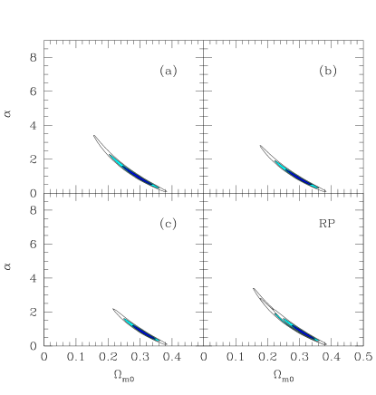
Figure 3: Confidence regions ($\Delta\chi^{2}=2.30,5.99,11.8$, corresponding to 1, 2 and 3$\sigma$ for a Gaussian distribution with two free parameters, respectively) for the parameters $\Omega_{m0}$ and $\alpha$ for the ordinary quintessence model with a Ratra-Peebles potential. The results are obtained with the simulated SNAP sample (dataset 1). Panel (a) refers to the constraints obtained by assuming the exact equation of state $w(z)$; panel (b) to the linear $w(z)$ approximation; panel (c) to the constant $w$ approximation. The final panel shows the superposition of the three cases.

In Figure 3 we show the confidence regions in the $\alpha-\Omega_{m0}$ plane obtained by fitting the OQ model with a RP potential to the dataset 1. As done also for the other fits described in this section, we fix the value of the Hubble constant to the ‘true’ value, $H_{0}=71$ km s^-1 Mpc^-1. In the panel (a) we show the results obtained with the exact equation of state. The best-fitting parameters are: $\alpha=0.91^{+0.44}_{-0.33}$ and $\Omega_{m0}=0.30^{+0.03}_{-0.04}$ at the $1\sigma$ level. They are consistent with the values assumed in the background cosmology, within the error limits. By comparing these results to those presented in the top-left panel of Figure 1, it is also evident the improvement with respect to the constraints obtained with the present SNIa data: the confidence regions are much narrower. Nonetheless, there is still a little degeneracy between $\alpha$ and $\Omega_{m0}$: to solve it will be useful to combine magnitude-redshift measurements to other cosmological tests (see, e.g., Balbi et al. 2003; Frieman et al. 2003; Jimenez et al. 2003; Caldwell & Doran 2003). The case of OQ model with a RP potential has already been examined by Podariu et al. (2001) for SNAP simulated data. Their confidence regions in the $\Omega_{m0}-\alpha$ plane look quite similar to ours, even if they considered a fiducial cosmology with $\alpha=4$ and $\Omega_{m0}=0.2$. A similar analysis has been carried out also by Eriksson & Amanullah (2002), who found an error on $\alpha$ which is approximately twice larger than ours. This difference is probably due to the different redshift distribution adopted.

In panel (b) of Figure 3 we show the confidence regions obtained when $\chi^{2}$ is computed using the linear approximation for $w(z)$, while in panel (c) we adopt a constant equation of state. The differences between the three considered cases (exact, linear and constant $w$) are evident also from the last panel, showing the superposition of the corresponding confidence regions. The best-fitting values we obtain are $\alpha=0.81^{+0.37}_{-0.29}$ and $\Omega_{m0}=0.31^{+0.03}_{-0.03}$ for the linear $w(z)$, and $\alpha=0.76^{+0.30}_{-0.26}$ and $\Omega_{m0}=0.31^{+0.02}_{-0.03}$ for the constant $w$, in both cases at $1\sigma$ level. The measured cosmological parameters are then consistent with the true values within the error limits. However, there seems to be a systematic tendency to underestimate $\alpha$, which increases when we decrease the accuracy used to describe the redshift evolution of $w$. Nevertheless, this systematic offset will be too small to be put in evidence by the SNAP data, even at the $1\sigma$ level. On the contrary, the approximations on $w(z)$ do not strongly influence the determination of $\Omega_{m0}$. Finally, we notice that, at the $1\sigma$ confidence level, the size of the errors for both $\alpha$ and $\Omega_{m0}$ appear to be smaller, i.e. systematically underestimated, when the linear and constant approximations are used instead of the exact solution.

We then perform the same kind of analysis by fitting OQ models with a SUGRA potential using the dataset 2. The results are shown in Figure 4. Looking at panel (a), which refers to the results obtained with the exact $w(z)$, it is evident that the SUGRA models present a strong degeneracy in $\alpha$, becoming larger with increasing values of $\alpha$. This was already pointed out by Brax & Martin (1999), who studied the dependence of $w_{0}$ on $\alpha$ in the same class of models. As a consequence, in this case it is impossible to determine the errors on the cosmological parameters. The confidence regions under the approximation of linear equation of state are shown in panel (b): they appear very similar to those displayed in panel (a). Instead, if we assume a constant $w$ (see panel c), the $1\sigma$ contour closes off, and we obtain: $\alpha=0.34^{+0.59}_{-0.33}$ and $\Omega_{m0}=0.32\pm 0.02$, which are marginally consistent with the true values $\alpha=1$ and $\Omega_{m0}=0.30$. Again, the last panel shows the superposition of the three cases. The situation slightly improves if we impose a Gaussian prior on $\Omega_{m0}$, namely $\Omega_{m0}=0.30\pm 0.05$. In fact we obtain $\alpha=0.95^{+6.25}_{-0.78}$ for the exact $w(z)$, $\alpha=0.49^{+1.23}_{-0.40}$ for the linear $w(z)$ and $\alpha=0.38^{+0.59}_{-0.26}$ for the constant $w$, all at the $1\sigma$ confidence level. All these values are consistent within the error limits with the original assumption of $\alpha=1$, but we see that by using the exact $w(z)$ the determination is very poor. Moreover, the use of linear or constant equation of state approximations could lead to an artificially higher precision in the determination of $\alpha$. For these reasons, we can conclude that even with SNAP it will not be possible to constrain OQ models with a SUGRA potential.

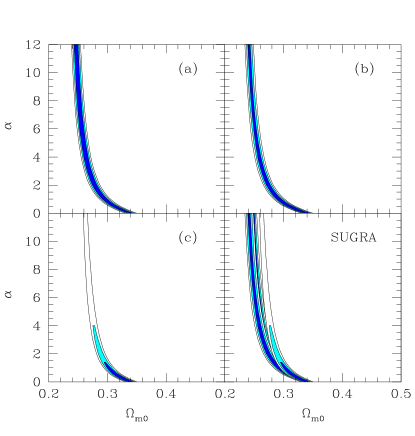
Figure 4: As Figure 3, but for the ordinary quintessence model with a SUGRA potential. The results are obtained with the simulated SNAP sample (dataset 2).

Finally, we use the dataset 3 to estimate the best-fitting parameters for EQ models with a RP potential. To this aim we determine the values of $\chi^{2}$ on a three-dimensional grid of values for the parameters $\alpha,\Omega_{m0}$ and $\xi$. In particular, we consider 100 values for $\xi$, regularly spaced between 0.001 to 0.100, as done in the previous section with the presently available SNIa data.

In Figure 5 we show the confidence regions in the $\Omega_{m0}-\alpha$ plane, obtained by minimizing (for each pair of these parameters) $\chi^{2}$ with respect to $\xi$. Panel (a) refers to the exact $w(z)$ case and can be directly compared to the bottom-left panel of Figure 1. Even if the regions become narrower, they are still larger than in the OQ models. It is possible to obtain the one-dimensional distribution separately for each of the three parameters, by minimizing $\chi^{2}$ with respect to the others. In this way we find that there is very little dependence of the minimized $\chi^{2}$ on $\xi$. Then, it is not possible to obtain useful constraints on this parameter (best fit value: $\xi=0.001$). Instead, we have $\alpha=0.95^{+0.44}_{-0.62}$ and $\Omega_{m0}=0.30^{+0.02}_{-0.03}$ at the $1\sigma$ level. This values are consistent with the true values ($\alpha=1$ and $\Omega_{m0}=0.3$) within the errors.

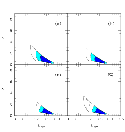
Figure 5: As Figure 3, but for the extended quintessence model with a Ratra-Peebles potential. The results are obtained with the simulated SNAP sample (dataset 3).

The confidence regions obtained using the approximated (linear and constant) equations of state (panels (b) and (c), respectively) are quite different from the previous ones, as it is evident from the superposition in the last panel. Again, there is no possibility to constrain $\xi$ (best fit values: $\xi=0.001$ for linear $w(z)$, and $\xi=0.003$ for constant $w$). For the remaining parameters we obtain: $\alpha=0.84^{+0.37}_{-0.51}$ and $\Omega_{m0}=0.31^{+0.02}_{-0.03}$ for the linear $w(z)$; and $\alpha=0.78^{+0.31}_{-0.46}$ and $\Omega_{m0}=0.32^{+0.01}_{-0.03}$ for constant $w$, at $1\sigma$ confidence level. These values are always consistent with the true ones, within the error limits.

As a final point, it is interesting to discuss how the confidence regions change if we impose the constraint coming from the time variation of the gravitational constant. The results are shown in Figure 6, where we draw the confidence regions in the $\Omega_{m0}-\alpha$ plane, obtained by minimizing $\chi^{2}$ with respect to $\xi$ and considering only the combination of the parameters for which the bounds on $G(t)$ are satisfied. This condition excludes combination of the parameters for which $\alpha$ and $\xi$ are high, and this is the main motivation for the differences with respect to Figure 5. Considering the case where the exact equation of state is used (panel (a)), we have $\alpha=0.95\pm{0.43}$ and $\Omega_{m0}=0.30\pm{0.03}$ at $1\sigma$: there is no significant change in the determination of these parameters with the imposition of the constraint. However, this time we are able to obtain an upper limit on $\xi$: $\xi<0.028$ at the $1\sigma$ level. This result is consistent with the assumed true value: $\xi=0.015$. Panel (b) refers to the linear $w(z)$ approximation, for which we derive $\alpha=0.84^{+0.37}_{-0.38}$, $\Omega_{m0}=0.31^{+0.02}_{-0.03}$ and $\xi<0.030$ at the $1\sigma$ level. Finally, panel (c) considers the constant $w$ approximation. In this case the resulting constraints are $\alpha=0.78^{+0.32}_{-0.33}$, $\Omega_{m0}=0.32^{+0.01}_{-0.03}$ and $\xi<0.030$ at the $1\sigma$ level. Again, all this values are consistent with the true ones.

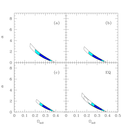
Figure 6: As Figure 3, but for the extended quintessence model with a Ratra-Peebles potential. The results are obtained by using the simulated SNAP sample (dataset 3) and imposing the upper bound on the time variation of the gravitational constant.

Up to now, we discussed the possibility of determining the quintessence parameters in the future data coming from SNAP by assuming intrinsic statistical errors only. Here we consider the impact of systematic errors on the previous results. Kim et al. (2004) define two general forms for them: uncorrelated systematic uncertainties and magnitude offsets. The first case represents a random dispersion which cannot be reduced below a given magnitude error over a finite redshift bin (here assumed to be $\Delta z=0.1$): possible examples are calibration errors and imperfect galaxy subtraction. The second case is a coherent shift acting as a bias on all SNIa magnitudes: selection effects as Malmquist bias or detector problems can produce this kind of effect.

In order to simulate irreducible systematics, we strictly follow Kim et al. (2004). In particular, for each redshift bin, containing $N_{SN}$ objects (see Figure 2), we add in quadrature to the intrinsic magnitude dispersion per SNIa (0.15 mag) an irreducible magnitude error $\Delta m$:

$$\sigma_{m}=\sqrt{\frac{0.15^{2}}{N_{SN}}+(\Delta m)^{2}}\ .$$ (10)

As in Kim et al. (2004), we consider two different possibilities for $\Delta m$: a constant value equal to 0.02 mag, which is the target of the SNAP mission, and a linear function increasing with redshift reaching at the maximum covered redshift, $z=1.7$, the maximum expected error for SNAP, 0.02 mag: $\Delta m=0.02(z/1.7)$. The resulting constraints on $\Omega_{m0}$ and $\alpha$ are shown in Figure 7 for the RP potential in the case of OQ and EQ (top-left and bottom-left panels, respectively). In both cases we show the 1$\sigma$ confidence regions when no priors are considered. The solid contour refers to the constraints obtained by considering statistical errors only; they are the same shown in the top-left panel of Figures 3 and 5. Dotted and dashed lines present the 1$\sigma$ regions when we include constant and linear irreducible systematic errors. We notice that systematics, as expected, extend the confidence regions, in particular in the direction of lower values for $\Omega_{m0}$ and higher values for $\alpha$. This effect is larger when we apply a constant $\Delta m$. In the OQ case, the best-fitting values for $\alpha$ is shifted up of 0.1 and the errors on the two variables are strongly correlated.

Then we investigate the effect of systematic magnitude offsets. First, we consider a constant shift of 0.02 mag, both positive and negative. The analysis (not shown in the figure) confirms the results obtained by Kim et al. (2004): in this case the best-fitting parameters are the true values with errors which are very similar to the ones obtained by considering statistical errors only, without any systematic biases. Then we consider a magnitude offset which is linearly proportional to the redshift as $\Delta m=\pm 0.03(z/1.7)$. The results for the same models previously considered (OQ and EQ with RP potential) are shown in the right panels of Figure 7. As discussed by Kim et al. (2004), an offset in magnitude can give best-fitting parameters which are wrong with smaller confidence regions, i.e. it is possible to have very accurate but wrong answers. This is exactly what is happening in our case. Considering a positive linear offset, we find the tendency to have confidence regions systematically shifted towards the left, while we have the opposite trend for negative magnitude shifts: the true values of the parameters $\Omega_{m0}$ and $\alpha$ are excluded at 1$\sigma$ confidence level. Finally we consider the presence of a possible mismatch between the calibration of low- and high-redshift SNIa. This is done by introducing a constant offset of $\pm 0.02$ mag to the 300 local objects only. The results (not shown in the figure for clarity) show that this kind of effect produces a small enlargement of the confidence regions, without introducing systematic biases in the parameter determination.

Figure 7: Effects of systematics errors on the 1$\sigma$ confidence regions for the parameters $\Omega_{m0}$ and $\alpha$ for the ordinary quintessence model with a Ratra-Peebles potential (upper panels) and extended quintessence model with a Ratra-Peebles potential (lower panels). The results are obtained with the simulated SNAP samples (datasets 1 and 3, respectively). Left panels show the effects of irreducible systematic uncertainties: dotted (dashed) contours refer to confidence regions obtained by including constant (linearly increasing) error $\Delta m$ (see text for details). Right panels present the effects of magnitude offsets: dotted (dashed) contours refer to a positive (negative) shift of 0.02 mag. In all panels, the solid curve represents the constraints obtained by assuming the presence of intrinsic statistical errors, only.

5 Conclusions

The main goal of this paper has been to discuss the possibility of using SNIa distances and redshifts to obtain reliable constraints on the parameters defining the quintessence models. In particular we considered extended quintessence models with Ratra-Peebles potential, and, for completeness, ordinary quintessence models with both Ratra-Peebles and SUGRA potentials.

As a first step, we studied the constraints which result from the analysis of the largest SNIa sample presently available (176 objects, coming from Tonry et al. 2003, Knop et al. 2003 and Blakeslee et al. 2003). To this purpose, we used the exact redshift evolution of the equation of state $w(z)$, as numerically determined, avoiding any approximation. Our results show that for ordinary quintessence with a SUGRA potential it is not possible to obtain significant limits on the potential exponent $\alpha$, because of the weak dependence of the equation of state on it. For ordinary quintessence with a Ratra-Peebles potential, it is possible to obtain an upper limit on $\alpha$: at the $1\sigma$ confidence level we find $\alpha\leq 0.83$. Our results, which are in agreement with a similar analysis made by Podariu & Ratra (2000) who used an older SNIa dataset, are consistent with a cosmological constant model, for which $\alpha=0$. We obtained a similar constraint for $\alpha$ when considering the extended quintessence models with Ratra-Peebles potential. Unfortunately, it is not possible to obtain useful constraints on the non-minimal coupling parameter $\xi$ between the scalar field and gravity.

We then discussed the potential improvement on the previous results when future SNIa samples, with a larger number of objects and more extended redshift coverage, will be available. To this purpose, we simulated SNIa datasets in different cosmological models, with the characteristics of the expected SNAP satellite observations (almost 2000 objects up to $z=1.7$).

For ordinary quintessence with a SUGRA potential, we found that it will still be difficult to constrain the parameters even with the SNAP SNIa data. Considering models with the Ratra-Peebles potential, both in extended and ordinary quintessence, our results suggest that $\alpha$ can be determined with an error $\raise-3.0pt\hbox{\hbox to0.0pt{\hbox{\hskip 3.0pt $\sim$}\hss}\raise 4.0pt\hbox{\hskip 3.0pt$<$}\ }0.6$ (at the $1\sigma$ significance level), while $\Omega_{m0}$ will be constrained with an error of approximately 0.03 (always at $1\sigma$). In extended quintessence models, even by imposing the upper bounds on the time variation of the gravitational constant, it will be possible to obtain only an upper limit on the coupling constant: $\xi<0.028$.

As a final issue, we discussed the systematic errors on the parameter estimates which originate if a constant or linear approximation is used for the equation of state, $w(z)$, instead of the exact redshift evolution. For all the considered quintessence models, the confidence regions obtained with these approximations look narrower than the exact ones. As a consequence, these approximations on $w(z)$ lead to a systematic underestimate of the errors. Nevertheless, the set of cosmological parameters determined by the fitting procedure are consistent with that used in the simulations. This means that the systematic errors induced by the assumed approximations are still smaller than the precision allowed on the cosmological parameters by SNAP, even at the $1\sigma$ confidence level.

References

- Aldering et al. (2002) Aldering, G., et al. 2002, Proc. of SPIE conference on Astronomical Instrumentation, 4836
- Allen et al. (2002) Allen, S.W., Schmidt, R.W., & Fabian, A.C. 2002, MNRAS, 334, L11
- Baccigalupi et al. (2000) Baccigalupi, C., Matarrese, S., & Perrotta, F. 2000, Phys. Rev. D, 62, 123510
- Bahcall (2000) Bahcall, N.A. 2000, Phys. Scripta, T85, 32
- Balbi et al. (2003) Balbi, A., Baccigalupi, C., Perrotta, F., Matarrese, S., & Vittorio, N. 2003, ApJ, 588, L5
- Bartolo (2000) Bartolo, N., & Pietroni, M. 2000, Phys. Rev. D, 61, 023518
- Bean (2001) Bean, R. 2001, Phys. Rev. D, 64, 123516
- Bennett et al. (2003) Bennett, C.L., et al. 2003, ApJS, 148, 1
- Binétruy et al. (1999) Binétruy, P. 1999, Phys. Rev. D, 60, 063502
- Blakeslee et al. (2003) Blakeslee, J.P., et al. 2003, ApJ, 589, 693
- Boisseau et al. (2000) Boisseau, B., Esposito-Farese, G., Polarski, D., & Starobinsky, A.A. 2000, Phys. Rev. Lett., 85, 2236
- Borgani et al. (2001) Borgani, S., et al. 2001, ApJ, 561, 13
- Brax & Martin (1999) Brax, P., & Martin, J. 1999, Phys. Lett. B, 468, 40
- Caldwell et al. (1998) Caldwell, R.R., Dave, R., & Steinhardt, P.J. 1998, Phys. Rev. Lett., 80, 1582
- Caldwell & Doran (2003) Caldwell, R.R., & Doran, M. 2003, preprint, astro-ph/0305334
- Chen et al. (2001) Chen, X.l., Scherrer, R.J., & Steigman,G. 2001, Phys. Rev. D, 63, 123504
- Chiba (1999) Chiba, T. 1999, Phys. Rev. D, 60, 083508
- Chiba (2001) Chiba, T. 2001, Phys. Rev. D, 64, 103503
- Coble et al. (1997) Coble, K., Dodelson, S., & Frieman, J.A. 1997, Phys. Rev. D, 55, 1851
- Damour (1998) Damour, T. 1998, Eur. Phys. J., C3, 113
- de Ritis et al. (2000) de Ritis, R., Marino, A.A., Rubano, C., & Scudellaro, P. 2000, Phys. Rev. D, 62, 043506
- Di Pietro & Claeskens (2003) Di Pietro, E., & Claeskens, J.-F. 2003, MNRAS, 341, 1299
- Eriksson & Amanullah (2002) Eriksson, M., & Amanullah, R. 2002, Phys. Rev. D, 66, 023530
- Faraoni (2000) Faraoni, V. 2000, Phys. Rev. D, 62, 023504
- Ferreira P.G. & M. Joyce (1998) Ferreira, P.G., & Joyce, M. 1998, Phys. Rev. D, 58, 023503
- Frieman et al. (2003) Frieman, J.A., Huterer, D., Linder, E.V., & Turner, M.S. 2003, Phys.Rev. D, 67, 083505
- Fujii (2000) Fujii, Y. 2000, Phys. Rev. D, 62, 044011
- Gasperini (2001) Gasperini, M. 2001, Phys. Rev. D, 64, 043510
- Gerke & Efstathiou (2002) Gerke, B.F., & Efstathiou, G. 2002, MNRAS, 335, 33
- Gillies (1997) Gillies, G.T. 1997, Rep. Prog. Phys., 60, 151
- Goliath et al. (2001) Goliath, M., Amanullah, R., Astier, P., Goobar, A., & Pain, R. 2001, A&A, 380, 6
- Gott et al. (2001) Gott, J.R., Vogeley, M.S., Podariu, S., & Ratra, B. 2001, ApJ, 549, 1
- Hamuy et al. (1996) Hamuy, M., et al. 1996, AJ, 112, 2408
- Hradecky et al. (2000) Hradecky, V., et al. 2000, ApJ, 543, 521
- Kim et al. (2004) Kim, A.G., Linder, E.V., Miquel, R., & Mostek, N. 2004, MNRAS, 347, 909
- Kneller & Steigman (2003) Kneller, J.,P., & Steigman, G. 2003, Phys. Rev. D, 67, 063501
- Knop et al. (2003) Knop, R.A., et al. 2003, ApJ, 598, 102
- Jimenez et al. (2003) Jimenez, R., Verde, L., Treu, T., & Stern, D. 2003, ApJ, 593, 622
- Padmanabhan & Choudhury (2003) Padmanabhan, T., & Choudhury, T.R. 2003, MNRAS, 344, 823
- Peebles & Ratra (2002) Peebles, P.J.E., & Ratra, B. 2003, Rev. Mod. Phys., 75, 599
- Percival et al. (2001) Percival, W.J., et al. 2001, MNRAS, 327, 1297
- Perlmutter et al. (1999) Perlmutter, S., et al. 1999, ApJ, 517, 565
- Perrotta et al. (1999) Perrotta, F., Baccigalupi, C., & Matarrese, S. 1999, Phys. Rev. D, 61, 023507
- Perrotta & Baccigalupi (2002) Perrotta, F., & Baccigalupi, C. 2002, Phys. Rev. D, 65, 123505
- Podariu et al. (2001) Podariu, S., Nugent, P., & Ratra, B. 2001, ApJ, 553, 39
- Podariu & Ratra (2000) Podariu, S. & Ratra, B. 2000, ApJ, 532, 109
- Ratra & Peebles (1988) Ratra, B., & Peebles, P.J.E. 1988, Phys. Rev. D, 37, 3406
- Reasenberg et al. (1979) Reasenberg, R.D., et al. 1979, ApJ, 234, L219
- Riazuelo (2002) Riazuelo, A., & Uzan,J.-P. 2002, Phys. Rev. D, 66, 023525
- Riess et al. (1998) Riess, A.G., et al. 1998, AJ, 116, 1009
- Spergel et al. (2003) Spergel, D.N., et al. 2003, ApJS, 148, 175
- Steinhardt et al. (1999) Steinhardt, P.J., Wang, L., & Zlatev, I. 1999, Phys. Rev. D, 59, 123504
- Tonry et al. (2003) Tonry, J.L., et al. 2003, ApJ, 594, 1
- Torres (2002) Torres, D.F. 2002, Phys. Rev. D, 66, 043522
- Uzan (1999) Uzan, J.-P. 1999, Phys. Rev. D, 59, 123510
- Uzan (2003) Uzan, J.-P. 2003, Rev. Mod. Phys. 75, 403
- Verde et al. (2002) Verde, L., et al. 2002, MNRAS, 335, 432
- Viana & Liddle (1998) Viana, P.T.P., & Liddle, A.R. 1998, Phys. Rev. D, 57, 674
- Weller & Albrecht (2001) Weller, J., & Albrecht, A. 2001, Phys. Rev. Lett., 86, 1939
- Weller & Albrecht (2002) Weller, J., & Albrecht, A. 2002, Phys. Rev. D, 65, 103512
- Will (1984) Will, C.M. 1984, Phys. Rep., 113, 345
- Zel’dovich (1968) Zel’dovich, Ya.B. 1968, Usp. Fiz. Nauk, 95, 209 [English translation in Sov. Phys. Usp. 11, 381 (1968)]