LUDWIG–MAXIMILIANS–UNIVERSITÄT MÜNCHEN

 
 
 
 
 
 
 
 
 
Cosmological Implications and Physical Properties of an X-Ray Flux-Limited Sample of Galaxy Clusters

x x
1. Gutachter: Prof. G. E. Morfill

2. Gutachter: Prof. R. Bender

Tag der mündlichen Prüfung: 10. Dezember 2001 x x
To my angel x

Chapter 0 Zusammenfassung

Ein Hauptziel dieser Arbeit ist die Bestimmung der mittleren Materiedichte im Universum. Die Materiedichte ist ein wesentlicher kosmologischer Parameter, der die Zukunft des Universums als Ganzem mitbestimmt. Es wurde dazu eine röntgenselektierte und röntgenflußbegrenzte Stichprobe der 63 röntgenhellsten Galaxienhaufen am Himmel (ohne das galaktische Band, genannt HIFLUGCS) zusammengestellt, basierend auf der ROSAT Himmelsdurchmusterung. Die Flußgrenze beträgt $2\,\times 10^{-11}\,{\rm ergs\,s^{-1}\,cm^{-2}}$ im Energieband $0.1-2.4\,{\rm keV}$. Anhand mehrerer Tests wurde gezeigt, daß eine hohe Vollständigkeit erreicht wurde. Diese Stichprobe kann, aufgrund der hoch angesetzten Flußgrenze, für eine Vielzahl von Anwendungen benutzt werden, die eine statistische Galaxienhaufenstichprobe benötigen, ohne Korrekturen an das effektive Durchmusterungsvolumen anbringen zu müssen.

Zur Bestimmung von Flüssen und physikalischen Haufenparametern wurden hauptsächlich tief belichtete pointierte Beobachtungen benutzt. Es wurde gezeigt, daß zwischen der Röntgenleuchtkraft und der gravitativen Masse eine enge Korrelation besteht, wobei HIFLUGCS und eine erweitere Stichprobe von 106 Galaxienhaufen benutzt wurde. Die Relation und die Streuung wurden quantifiziert mit Hilfe verschiedener Anpassungsmethoden. Ein Vergleich mit einfachen und erweiterten theoretischen und numerischen Vorhersagen zeigt insgesamt Übereinstimmung. In großen Röntgenhaufendurchmusterungen oder Simulationen dunkler Materie kann diese Relation direkt für Konvertierungen zwischen der Röntgenleuchtkraft und der gravitativen Masse angewendet werden.

Daten des Galaxienhaufens Abell 1835, aufgenommen während der ‘Performance Verification’ Phase des kürzlich gestarteten Röntgensatellitenobservatoriums XMM-Newton wurden ausgewertet, um die in dieser Arbeit benutzte Annahme, daß das Intrahaufengas in den äußeren Gebieten des Haufens isotherm ist, zu testen. Es wurde gefunden, daß das gemessene äußere Temperaturprofil konsistent mit einem isothermen Profil ist. In den inneren Regionen wurde ein klarer Abfall der Gastemperatur um einen Faktor zwei gefunden.

Physikalische Eigenschaften der Galaxienhaufenstichprobe wurden untersucht, indem Relationen zwischen verschiedenen Haufenparametern analysiert wurden. Die Gesamteigenschaften sind gut verstanden, aber im Detail ergaben sich Abweichungen von einfachen Erwartungen. Es wurde gefunden, daß der Anteil der Gasmasse an der Gesamtmasse nicht als Funktion der Temperatur des Intrahaufengases variiert. Für Galaxiengruppen ($k_{\rm B}T_{\rm X}\lesssim 2$ keV) wurde jedoch ein steiler Abfall dieses Anteils gefunden. Keine klare Tendenz für eine Variation des Oberflächenhelligkeitsprofils, d.h. $\beta$, als Funktion der Temperatur wurde beobachtet. Es wurde gefunden, daß die Relation zwischen der Röntgenleuchtkraft und der Temperatur steiler als von einfachen selbstähnlichen Modellen erwartet verläuft, wie bereits in früheren Arbeiten festgestellt. Allerdings wurden keine klaren Abweichungen von der Form eines Potenzgesetzes bis zu einer gemessenen Gastemperatur $k_{\rm B}T_{\rm X}=0.7$ keV gefunden. Die hier gefundene Relation zwischen der Gesamtmasse und der Temperatur ist steiler als von selbstähnlichen Modellen erwartet und die Normierung ist niedriger im Vergleich zu hydrodynamischen Simulationen, in Übereinstimmung mit früheren Resultaten. Vorgeschlagene Szenarien, darunter Heiz- und Kühlprozesse, zur Beschreibung dieser Abweichungen und Schwierigkeiten bei dem Beobachtungsprozeß wurden dargestellt. Es scheint, daß eine Überlagerung verschiedener Effekte, möglicherweise inklusive einer Veränderung der mittleren Entstehungsrotverschiebung als Funktion der Galaxienhaufenmasse, benötigt ist, um die hier vorgelegten Beobachtungen zu beschreiben.

Unter Benutzung von HIFLUGCS wurde die gravitative Massenfunktion in dem Massenintervall $3.5\times 10^{13}<M_{200}<5.2\times 10^{15}\,h_{50}^{-1}\,M_{\odot}$ bestimmt. Vergleich mit Press–Schechter Massenfunktionen führte dazu, daß die mittlere Materiedichte im Universum und die Amplitude der Dichtefluktuationen eng eingegrenzt werden konnten. Das große überdeckte Massenintervall erlaubte eine individuelle Eingrenzung der Parameter. Im einzelnen wurde gefunden, daß $\Omega_{\rm m}=0.12^{+0.06}_{-0.04}$ und $\sigma_{8}=0.96^{+0.15}_{-0.12}$ (90 % Konfidenzintervall statistische Unsicherheit). Dieses Resultat ist konsistent mit zwei weiteren unterschiedlichen Abschätzungen für $\Omega_{\rm m}$ in dieser Arbeit. Der mittlere Anteil des Intrahaufengases an der Gesamtmasse von Galaxienhaufen, bestimmt mit Hilfe einer erweiterten Stichprobe von 106 Haufen, kombiniert mit Vorhersagen der Theorie der Elemententstehung deutet an, daß $\Omega_{\rm m}\lesssim 0.34$. Das Masse zu Licht Verhältnis in den Haufen multipliziert mit der mittleren Leuchtkraftdichte impliziert $\Omega_{\rm m}\approx 0.15$. Eine Anzahl von Tests auf systematische Unsicherheiten wurde duchgeführt, darunter ein Vergleich der Press–Schechter Massenfunktion mit den neuesten Resultaten von großen Vielteilchenrechnungen. Diese Tests ergaben Abweichungen kleiner als die statistischen Unsicherheiten. Zum Vergleich wurden die Werte der besten Anpassung von $\Omega_{\rm m}$ für gegebenes $\sigma_{8}$ bestimmt, was zu der Relation $\sigma_{8}=0.43\,\Omega_{\rm m}^{-0.38}$ führte.

Die Massenfunktion wurde integriert, um den Anteil an der gesamten gravitativen Masse im Universum zu bestimmen, der in Galaxienhaufen enthalten ist. Normiert auf die kritische Dichte ergab sich $\Omega_{\rm Cluster}=0.012^{+0.003}_{-0.004}$ für Galaxienhaufenmassen größer als $6.4^{+0.7}_{-0.6}\times 10^{13}\,h_{50}^{-1}\,M_{\odot}$. Dies impliziert mit dem hier bestimmten Wert für $\Omega_{\rm m}$, daß sich ca. 90 % der Gesamtmasse des Universums außerhalb von virialisierten Haufenregionen befindet. Auf ähnliche Weise wurde gefunden, daß der Anteil des Intrahaufengases an der Gesamtmasse des Universums mit $\Omega_{\rm b,Cluster}=0.0015^{+0.0002}_{-0.0001}\,h_{50}^{-1.5}$ für Gasmassen größer als $6.9^{+1.4}_{-1.5}\times 10^{12}\,h_{50}^{-5/2}\,M_{\odot}$ sehr klein ist.

Contents

1. 0 Zusammenfassung
2. 1 Introduction
3. 2 Theoretical Background
   1. 2.1 Galaxy Clusters
      1. 2.1.1 Cluster Galaxies
      2. 2.1.2 Intracluster Gas
         1. 2.1.2.1 Gas Density
         2. 2.1.2.2 Gas Temperature
      3. 2.1.3 Dark Matter
      4. 2.1.4 Relativistic Electrons
   2. 2.2 Cosmology
      1. 2.2.1 Some Basics
      2. 2.2.2 Practical Formulae
      3. 2.2.3 Mass Function
         1. 2.2.3.1 Observational Determination
         2. 2.2.3.2 Theoretical Determination
   3. 2.3 Instruments
4. 3 Sample
5. 4 Reduction and Analysis
   1. 4.1 Flux Determination
   2. 4.2 Mass Determination
6. 5 Temperature Structure of Abell 1835
   1. 5.1 Motivation
   2. 5.2 Data Reduction and Analysis
   3. 5.3 Results and Discussion
   4. 5.4 Conclusions
7. 6 Results
   1. 6.1 Mass–Luminosity Relation
   2. 6.2 Intracluster Gas Fraction
      1. 6.2.1 Variation of Gas Fraction with Mass
      2. 6.2.2 Variation of Gas Fraction with Radius
   3. 6.3 Relations between Shape Parameters, Temperature, Luminosity, and Mass
   4. 6.4 Mass Function
8. 7 Discussion
   1. 7.1 Sample Completeness
   2. 7.2 Comparison of Mass Determinations
      1. 7.2.1 X-Ray Masses
      2. 7.2.2 Optical Masses
   3. 7.3 Mass–Luminosity Relation
   4. 7.4 Intracluster Gas Fraction
   5. 7.5 Relations between Shape Parameters, Temperature, Luminosity, and Mass
   6. 7.6 Mass Function
      1. 7.6.1 Comparison to Previous Estimates
      2. 7.6.2 Comparison to Predicted Mass Functions
      3. 7.6.3 Mass Function estimated using $L_{\rm X}$–$M_{\rm tot}$ Relation
   7. 7.7 Total Gas and Gravitating Mass in Clusters
9. 8 Conclusions
10. 9 Summary
11. A Acknowledgements

Chapter 1 Introduction

Observational cosmology is currently a very active field of astronomical research. The aim is the determination of the past, present, and future status of the universe. Optical observations of the magnitude–redshift relation of distant supernovae (SNe) indicate an accelerating universe, i.e. $2\,\Omega_{\Lambda}>\Omega_{\rm m}$ (e.g., Perlmutter et al., 1999), where $\Omega_{\rm m}$ is the normalized mean matter density of the universe and $\Omega_{\Lambda}$ the normalized cosmological constant. In the microwave regime, measurements of the fluctuations in the Cosmic Microwave Background (CMB) from recent satellite and ballon borne experiments indicate a flat geometry, i.e. $\Omega_{\rm m}+\Omega_{\Lambda}=1$ (e.g., de Bernardis et al., 2000). From the X-ray side, clusters of galaxies, as the most massive collapsed objects known in the universe, are the ideal and most commonly used cosmological probes and indicate a low density universe, i.e. $\Omega_{\rm m}<1$, almost independent of $\Omega_{\Lambda}$.

The SNe and CMB measurements clearly are very important cosmological tests, nevertheless both suffer from inherent problems. The SNe are used as standard candles but the detailed physical processes that take place during a SN explosion are not well understood even at redshift $z\approx 0$. Furthermore additional dimming of the apparent brightness caused by gas and dust in the host galaxy of a distant SN is difficult to quantify. The presence of outliers in the SN distribution is worrying and a large number of objects is needed to clearly identify such events (early results based on a smaller number of objects actually seemed to indicate $\Omega_{\Lambda}\approx 0$, Perlmutter et al., 1997). CMB measurements yield information on the state of the universe at $z\sim 1000$, whereas galaxy clusters yield information from relatively low redshifts ($0<z\lesssim 1$). It is thus important to take advantage of an independent method using galaxy clusters as performed in this work.

Galaxy clusters can be used in a variety of ways to constrain cosmological parameters. For instance one may determine the typical mass to light ratio in clusters and multiply it by the measured total luminosity density to determine the mean mass density (e.g., Bahcall et al., 1995, and Sect. 7.3). The underlying assumption is that the mass to light ratio in clusters is a good approximation to the mass to light ratio of the universe. Another method uses the amount of mass contained in the intracluster gas as compared to the total gravitational cluster mass to set an upper limit on $\Omega_{\rm m}$ by comparison to predictions for the baryon density from the theory of nucleosynthesis (e.g., White et al., 1993b , and Sect. 7.6). This approach assumes that the gas fraction in clusters resembles the baryon fraction in the universe. Furthermore within the framework of hierarchical structure formation – small objects, e.g. galaxies, form first and assemble to larger structures, e.g. galaxy clusters, afterwards under the influence of gravity – the merger rate depends also on $\Omega_{\rm m}$ (e.g., Lacey and Cole, 1993). A comparison of observed cluster substructure frequencies with predictions of specific models therefore allows in principal to put constraints on important parameters (e.g., Schuecker et al., 2001c ). Moreover within this framework analytical prescriptions have been developped, which allow statistical predictions of the cosmic mass distribution for given cosmological models (e.g., Press and Schechter, 1974; Bond et al., 1991; Bower, 1991; Lacey and Cole, 1993; Kitayama and Suto, 1996; Schuecker et al., 2001a ). These predictions have been tested against a number of $N$-body simulations and in general good agreement has been found over wide mass ranges (e.g., Efstathiou et al., 1988; Lacey and Cole, 1994; Governato et al., 1999; Jenkins et al., 2001). In this work the mean density of the universe is estimated utilizing three different methods. Most weight is given to the method, where the local cluster mass distribution is determined and compared to predictions, because the mass distribution is the most fundamental predicted quantity from cosmological models and simulations of structure formation.

The observed galaxy cluster mass function, i.e. the cluster number density as a function of mass, is particularly sensitive to the fundamental cosmological parameters $\Omega_{\rm m}$ and amplitude of the density fluctuations (e.g., Henry and Arnaud, 1991; Bahcall and Cen, 1992). Previous local galaxy cluster mass functions have been derived by Bahcall and Cen, (1993), Biviano et al., (1993), Girardi et al., 1998a , and Girardi and Giuricin, (2000, for galaxy groups). Bahcall and Cen, (1993) used the galaxy richness (measure of the cluster galaxy content, Sect. 2.1.1) to relate to cluster masses for optical observations and an X-ray temperature–mass relation to convert the temperature function given by Henry and Arnaud, (1991) to a mass function. Biviano et al., (1993), Girardi et al., 1998a , and Girardi and Giuricin, (2000) used velocity dispersions for optically selected samples to determine the mass function. Here a different strategy is used for the determination of the mass function. A statistical cluster sample is constructed taking advantage of the availability of an all-sky X-ray imaging survey. Furthermore the large number of archival cluster observations is exploited allowing detailed gravitational mass determinations through X-ray imaging and X-ray spectroscopy for the clusters included in the sample.

The overall physical processes determining the main properties of clusters and their appearance in X-rays are well understood. Intracluster gas (ICG) is trapped and heated to $10^{7}$–$10^{8}\,\rm K$ in the cluster gravitational potential. Thermal bremsstrahlung emission from this ICG makes clusters luminous X-ray sources. Only bright quasars exceed the typical cluster luminosities of $\sim 10^{45}\,{\rm ergs\,s^{-1}}$.

The X-ray luminosity is well correlated with cluster mass (as will be shown in this work) as opposed to the measured galaxy richness, which has often been employed as selection criterium for optically selected cluster samples. Therefore X-ray selection effectively selects galaxy clusters by their mass. This property is vital for the construction of the mass function.

The ROSAT All-Sky Survey (RASS), being the only all-sky survey carried out by an X-ray satellite with imaging capabilities to date (e.g., Trümper, 1993), has yielded a wealth of newly discovered X-ray sources (e.g., Voges et al., 1999). A variety of galaxy cluster catalogs, together covering the whole sky, have been homogeneously built from the RASS (see references in Chap. 3). These catalogs are utilized in this work for the construction of an X-ray selected and X-ray flux-limited sample of the brightest galaxy clusters in the sky (excluding a strip of $\pm 20$ deg from the galactic plane, in order to ensure a high completeness). To perform a detailed characterization of the thereby selected galaxy clusters, including the determination of the gravitational cluster mass, high quality (deep exposure) pointed observations of the PSPC detector onboard the ROSAT observatory are then analyzed and intracluster gas temperatures, mainly determined with the ASCA satellite because of its superior spectral resolution and larger sensitive energy range compared to ROSAT, are compiled from the literature.

Within the framework of hierarchical structure formation the properties of galaxy clusters are also expected to follow certain scaling relations and simulations have shown that scaled dark matter profiles look similar (e.g., Navarro et al., 1995). Despite the well established overall understanding of galaxy clusters, in detail deviations from this picture have been found from observationally accessible quantities, e.g., by the relation between X-ray luminosity and intracluster gas temperature (e.g., David et al., 1993), and the gas properties in the center of groups of galaxies (e.g., Ponman et al., 1999). A variety of models has been suggested to explain these deviations (Sect. 7.4). Tests of detailed predictions of these models unfortunately are still compromised by observational difficulties. For instance the observed gas mass fraction has been found in the recent literature to either stay constant, decrease, or increase as a function of cluster temperature (Sect. 7.4). The homogeneously selected and analyzed cluster sample presented here, comprising more than 100 galaxy groups and clusters, is therefore used to determine physical quantities like the X-ray luminosity, intracluster gas density distribution, temperature, and mass, as well as the gravitational mass over a wide temperature range from 0.7 to 13 keV. The relations between these quantities are analyzed and compared to predicted relations.

The structure of this work is as follows. In Chap. 2 the different components of galaxy clusters are introduced with emphasis on the gas and gravitational mass determination. Furthermore some relevant cosmological background is given, including the calculation of model mass functions. Last not least the observing instruments are briefly described with most of the weight assigned to ROSAT and the RASS, according to their importance for this work. The sample construction is described in Chap. 3. The details of the data reduction and analysis, and the determination of relevant quantities are given in Chap. 4. The gas temperature structure is very important for the X-ray mass determination of clusters. Therefore due to its importance for the present investigation the temperature profile for an example cluster is determined using brandnew data from the X-ray satellite mission XMM-Newton, which are in many respects superior to ROSAT and ASCA data (Chap. 5). Before the mass function is determined in Chap. 6 – being the first galaxy cluster mass function constructed from an X-ray selected and X-ray flux-limited sample based on the RASS – the physical properties of the cluster sample are examined. Especially the correlation between X-ray luminosity and gravitational mass is of major importance here. In Chap. 7 tests of the sample completeness are performed and the cluster masses determined here are compared to independent determinations. The relations found between physical cluster properties are discussed. The mass function is compared to previous determinations and the cosmological implications of this mass function are presented, including a fit to model mass functions. Tight constraints on $\Omega_{\rm m}$ are derived. Previous work indicated that the mass fraction contained in galaxy clusters may comprise already a fairly large fraction of the total mass in the universe (e.g., Fukugita et al., 1998). The well determined mass function given in this work is therefore used to determine the mass fraction in bound objects above a minimum mass to test these results.

Chapter 2 Theoretical Background

2.1 Galaxy Clusters

Clusters of galaxies are believed to consist of four main components. As indicated by the name galaxy clusters have been discovered as conglomerates of galaxies. The space between these galaxies is not empty but contains huge amounts of intracluster gas (ICG). The largest portion of the total gravitating mass in clusters, however, exists in the form of dark matter. A possible forth component is a population of highly relativistic electrons, i.e. electrons having velocities close to the speed of light. Some characteristics of these components are briefly summarized in this Section (for a review see, e.g., Sarazin, 1986). Since this work mainly deals with the intracluster gas and its implications for the dark matter content, these two components are awarded more attention.

2.1.1 Cluster Galaxies

How many galaxies make a cluster? An assembly of more than 4–5 galaxies is called a galaxy group (e.g., Hickson, 1982), $\sim 100$ galaxies make a cluster, and $\sim 1\,000$ galaxies a rich cluster. These rough numbers exclude ‘dwarf’ galaxies, which are difficult to count due to their faintness, except in the most nearby clusters. Abell, (1958) introduced the richness as a measure for clusters. The richness is determined by the number of galaxies above background fulfilling certain criteria. The two main criteria are that only galaxies be counted that a) are not more than two magnitudes fainter than the third brightest member galaxy, and b) have a projected distance from the center not larger than the Abell radius $r_{\rm A}\equiv 3\,h_{50}^{-1}\,{\rm Mpc}$.

The galaxy population in clusters differs from the field population, i.e. galaxies not contained in clusters, especially in the following properties.

• Morphology. The relative number of elliptical (E) and lens shaped (S0) galaxies in clusters is larger and the relative number of spiral galaxies is smaller than in the field (e.g., Dressler, 1984; Oemler Jr., 1992).

• Color. Spirals and irregular galaxies in clusters are redder on average than the same types in the field (e.g., Oemler Jr., 1992).

• Gas content. Especially spirals close to the cluster center contain less amounts of neutral hydrogen than spirals in the field (e.g., Cayatte et al., 1990).

• cD galaxies. These giant elliptical galaxies are found in the center of most groups and clusters. The most striking property of these cD galaxies is a very extended halo of low surface brightness (e.g., Matthews et al., 1964).

2.1.2 Intracluster Gas

The intracluster gas is the most massive visible component of galaxy clusters. Its mass exceeds the (gravitating) mass contained in the cluster galaxies by a factor of $\sim$ 2–5. The temperature, $T_{\rm gas}$, of the ICG is in the range $1\lesssim k_{\rm B}T_{\rm gas}\lesssim 15\,\rm keV$ (here $1\,{\rm keV}$ corresponds to $1.16045\times 10^{7}\,\rm K$). The central gas number density, $n_{\rm gas}(0)$, is in the range $10^{-3}$–$10^{-1}\rm\,particles\,cm^{-3}$. The collisionally ionized plasma is optically thin and emits thermal radiation in X-rays. For $T_{\rm gas}\gtrsim 2\,\rm keV$ the main component is bremsstrahlung (free-free transitions), for lower temperatures recombination (free-bound transitions) and line emission (bound-bound transitions) become more important. The emissivity depends on the density². A parameterized radial gas density distribution can be determined analytically from the observed surface brightness distribution. Numerical deprojections using onion shell models are also applied (e.g., Fabian et al., 1981). The procedure of the analytic deprojection is outlined in Sect. 2.1.2.1. The observational determination of $T_{\rm gas}$ is described in Sect. 2.1.2.2.

2.1.2.1 Gas Density

Assuming King’s (1962) approximation to an isothermal sphere for the galaxy density distribution, $\rho_{\rm gal}$, leads to an analytical representation of the radial gas density distribution (the ‘standard $\beta$ model’, e.g., Cavaliere and Fusco-Femiano, 1976; Sarazin and Bahcall, 1977; Gorenstein et al., 1978; Jones and Forman, 1984; Sarazin, 1986),

$$\rho_{\rm gas}(r)=\rho_{\rm gas}(0)\left(1+\frac{r^{2}}{r_{\rm c}^{2}}\right)^{-\frac{3}{2}\beta}\,,$$ (2.1)

by using $\rho_{\rm gas}\propto\rho_{\rm gal}^{\beta}$, as implied by assuming the gas to be ideal, isothermal, and in hydrostatic equilibrium, and the galaxies to have an isotropic velocity dispersion, where $\beta$ denotes the ratio of the specific kinetic energies of the galaxies and the gas. The shape of the gas density distribution is therefore determined by the core radius, $r_{\rm c}$, and the shape parameter, $\beta$. The asumptions leading to the $\beta$ model may be violated in detail. The justification for its wide spread usage comes from the fact that the surface brightness profile derived from it (see below) represents the measured profile well in the relevant radial ranges. The gas mass,

$$M_{\rm gas}(<r)=4\pi\int_{0}^{r}\rho_{\rm gas}(r)r^{2}dr\,,$$ (2.2)

may for illustrative purposes be approximated for large radii and small $\beta$ values by

$$M_{\rm gas}(<r)\approx\frac{4\pi\rho_{\rm gas}(0)r_{\rm c}^{3}}{-3\beta+3}\left(\frac{r}{r_{\rm c}}\right)^{-3\beta+3}\quad:\quad\frac{r}{r_{\rm c}}\gg 1\wedge\beta<1\,.$$ (2.3)

The main constituents of the ICG are Hydrogen and Helium, where a good approximation for the number densities is $n_{\rm He}=n_{\rm H}/10$. Due to the high temperature the gas can be considered completely ionized and the mean molecular weight including the electrons

$$\mu\approx\frac{1+2\sum\limits_{Z>1}w_{\rm Z}Z}{2+\sum\limits_{Z>1}w_{\rm Z}(Z+1)}\,,$$ (2.4)

where $Z$ is the atomic number and $w_{\rm Z}$ the relative weight (e.g., here $w_{2}=0.1$ and $w_{\rm Z}=0$ for $Z>2$). Therefore one has $\mu\approx 0.61$ and

$$\rho_{\rm gas}\approx 1.17\,n_{\rm e}\,m_{\rm p}\,.$$ (2.5)

Because of this proportionality between electron number density, $n_{\rm e}$, and gas density it follows from (2.1)

$$n_{\rm e}(r)=n_{\rm e}(0)\left(1+\frac{r^{2}}{r_{\rm c}^{2}}\right)^{-\frac{3}{2}\beta}\,.$$ (2.6)

Before the connection between the observable surface brightness and the gas density is made a few more important quantities are introduced. The luminosity, $L_{\nu}$, i.e. the energy radiated per unit time at the frequency $\nu$ is given by

$$L_{\nu}=\int_{V}\epsilon_{\nu}\,dV\,,$$ (2.7)

where the emissivity

$$\epsilon_{\nu}=n_{\rm e}\,n_{\rm H}\,\Lambda_{\nu}(T_{\rm gas},A)\,.$$ (2.8)

The emission coefficient, $\Lambda_{\nu}$, mainly depends on the gas temperature and metallicity, $A$. However, it varies only weakly in the energy range where ROSAT is sensitive (e.g., Böhringer, 1995), for the relevant cluster gas temperature range (2–10 keV). The emission measure is defined as

$$E_{\rm m}\equiv\int_{V}n_{\rm e}^{2}\,dV\,.$$ (2.9)

For the X-ray surface brightness, i.e. the number of photons detected in a defined energy range per unit time and per unit solid angle, one has

$$S_{\rm X}\propto\int_{-\infty}^{\infty}n_{\rm e}^{2}\,dl\,,$$ (2.10)

where the integration is along the line of sight ($l=0$ at the cluster center). With (2.6) it follows

$$S_{\rm X}\propto\int_{-\infty}^{\infty}\left(1+\frac{r^{2}}{r_{\rm c}^{2}}\right)^{-3\beta}dl\,.$$ (2.11)

This integral can be reduced to a form solved in, e.g., Bronstein and Semendjajew, (1980, Integral No. 39) and one finds

$$S_{\rm X}(R)=S_{\rm X}(0)\left(1+\frac{R^{2}}{r_{\rm c}^{2}}\right)^{-3\beta+\frac{1}{2}}\,,$$ (2.12)

where $R$ denotes the projected distance from the cluster center. $S_{\rm X}(0)$ depends on $n_{\rm e}(0)$, $r_{\rm c}$, $\beta$, $\Lambda_{\nu}(T_{\rm gas},A)$, and redshift, $z$. Equation (2.12) is used as a fitting formula to fit the observed surface brightness profile. With the obtained fit parameter values for $S_{\rm X}(0)$, $r_{\rm c}$, and $\beta$ the gas density profile can be determined with (2.1), where $\rho_{\rm gas}(0)$ is obtained from (2.5). The important step for the determination of the gas density distribution from (2.12) is the emission mechanism (2.8), which is well understood. The $\beta$ model has been applied successfully already for many years, but also other models have been used, e.g., gas density distributions (e.g., Makino et al., 1998) based on the Navarro-Frenk-White profile (Navarro et al., 1996, 1997), which is a fitting formula that represents well the cluster dark matter distribution found in $N$-body simulations for varying cosmological models (but see Sect. 2.1.3).

Some clusters exhibit a central excess emission not well approximated by (2.12). To get a more accurate decription of the gas density profile in such cases, a double $\beta$ model has been used by different authors (e.g., Ikebe et al., 1996; Mohr et al., 1999) to fit the data, where the surface brightness takes the form $S_{\rm X}=S_{\rm X}{{}_{,1}}+S_{\rm X}{{}_{,2}}$. The motivation is to have one component accounting for the central excess emission and the other component accounting for the overall cluster emission. It follows from the proportionality (2.10) that the gas density can then be determined from $n_{\rm e}=[n_{\rm e}{{}_{,1}}^{2}+n_{\rm e}{{}_{,2}}^{2}]^{1/2}$. It has been shown, however, that the gas mass determination is not biased by the presence of central excess emission for instance by Reiprich, (1998), who compared gas masses determined using single and double $\beta$ models.

It is worth noting that a new method to determine the gas mass in clusters is becoming more and more important (e.g., Carlstrom et al., 1996), which uses the distortion of the CMB photon spectrum caused by inverse Compton scattering on the hot ICG, the Sunyaev–Zeldovich effect (Zeldovich and Sunyaev, 1969; Sunyaev and Zeldovich, 1970).

2.1.2.2 Gas Temperature

When clusters of galaxies had been discovered as strong X-ray emitters more than 30 years ago (for references of the first detections and interpretations see, e.g., Sarazin, 1986) several possible emission mechanisms were discussed. The detection of line emission due to highly ionized iron in the X-ray spectra (e.g., Mitchell et al., 1976; Serlemitsos et al., 1977), however, made clear that the major contribution is thermal emission. The main mechanism to heat the intracluster gas to the high temperatures observed is expected to be shocks. These shocks are caused by the gravitational assembling of the cluster from subunits.

The electron temperature can be determined by fitting model spectra (folded with the instrument response) to the observed X-ray spectra (Chap. 5). Assuming electrons and ions to be in thermal equilibrium this X-ray temperature corresponds to the gas temperature. Within $2\,h_{50}^{-1}\,{\rm Mpc}$ Fox and Loeb, (1997) have shown that this assumption should be satisfied. Since X-ray temperatures are seldom available for radii larger than $2\,h_{50}^{-1}\,{\rm Mpc}$ they should generally be good indicators of the gas temperatures. Several spectral codes for hot, optically thin plasmas have been published (e.g., Raymond and Smith, 1977; Mewe et al., 1995; Smith et al., 2001).

The general dependence of the gas temperature on the distance from the cluster center has been discussed controversely recently utilizing data from various satellites (e.g., Fukazawa, 1997; Markevitch et al., 1998; Irwin et al., 1999; White, 2000; Irwin and Bregman, 2000). Including the latest findings from XMM-Newton (M. Arnaud, private communication; Chap. 5) the gas seems to be isothermal out to at least half the virial radius. In the very central part, where processes related to cooling flows (e.g., Fabian, 1994, and references therein) or cD galaxies (e.g., Mulchaey, 2000; Makishima et al., 2001, and references therein) may become important, a temperature drop is often found.

2.1.3 Dark Matter

The sum of the mass of all visible galaxies does by far not provide enough gravitational attraction to hold these galaxies in a cluster (e.g., Zwicky, 1933). Now, after the detection of the large amounts of gas present in clusters, does the gas mass suffice to retain the galaxies and the gas? The answer is no. Assuming the laws of gravitation to be the same at the distance and at the scale of clusters still about 3/4 of the mass is ‘missing’.

Several candidates for this ‘dark’ matter have been and are being discussed. While, for instance, observations of the large scale clustering of galaxies rule out neutrinos (candidates for Hot Dark Matter, HDM) as forming the only component of the dark matter (e.g., White et al., 1983), the recent strong evidence that neutrinos with finite rest mass do exist (e.g., Fukuda et al., 1998) leaves the possibility that at least part of the missing mass is provided by neutrinos. One of the frequently cited possible Cold Dark Matter (CDM) particles is the axion (e.g., Overduin and Wesson, 1993); also the heavier neutralino and gravitino are often discussed (e.g., Overduin and Wesson, 1997).

Clusters of galaxies form a natural laboratory – obviously quite a bit larger than any experiment that could be built on Earth – filled abundantly with dark matter particles and may therefore be utilized to actually place constraints on the nature of dark matter candidates. Recently, e.g., Spergel and Steinhardt, (2000) suggested that elastic collisions of weakly self interacting particles may provide an explanation for the discrepancy between simulated CDM halos and observations of galaxies and clusters of galaxies. The discrepancy arises when radial dark matter profiles from simulations of collisionless dark matter particles (e.g., Navarro et al., 1996) are compared to dark matter profiles indicated by rotation curves of dwarf galaxies (e.g., Burkert, 1995; but see Kravtsov et al., 1998) and by radial gas density profiles of clusters (e.g., Makino et al., 1998).

A more empirical dark matter density profile suggested by Burkert, (1995) better reproduces the data on dwarf galaxies and also on the gas density distribution in clusters (e.g., Wu and Xue, 2000).

This work mainly concentrates on the observational determination of the amount of gravitational mass. Therefore in this paragraph a widely used method for this determination, which has also been used here, is decribed. The basic assumption is that the ICG is in hydrostatic equilibrium, i.e.

$$\frac{dP_{\rm gas}(r)}{dr}=\frac{-\rho_{\rm gas}(r)GM_{\rm tot}(<r)}{r^{2}}\,,$$ (2.13)

where $P_{\rm gas}$ represents the gas pressure, $G$ the gravitational constant, and $M_{\rm tot}$ the cluster’s gravitational mass. With the ideal gas equation,

$$P_{\rm gas}=\frac{k_{\rm B}}{\mu m_{\rm p}}\rho_{\rm gas}T_{\rm gas}\,,$$ (2.14)

this leads to

$$M_{\rm tot}(<r)=-\frac{k_{\rm B}T_{\rm gas}(r)r^{2}}{\mu m_{\rm p}G}\left(\frac{1}{\rho_{\rm gas}(r)}\frac{d\rho_{\rm gas}(r)}{dr}+\frac{1}{T_{\rm gas}(r)}\frac{dT_{\rm gas}(r)}{dr}\right)\,.$$ (2.15)

Inserting (2.1) and, based on the recent findings of XMM-Newton (Sect. 2.1.2.2), assuming the cluster gas to be isothermal yields

$$M_{\rm tot}(<r)=\frac{3k_{\rm B}T_{\rm gas}r^{3}\beta}{\mu m_{\rm p}G}\left(\frac{1}{r^{2}+r_{\rm c}^{2}}\right)\,.$$ (2.16)

This equation is used throughout for the determination of the gravitational mass. The influence of a possible non isothermality of the cluster gas on the results is discussed in Chap. 7. The assumption of hydrostatic equilibrium can be motivated by considering that the sound speed in the ICG $C_{\rm s}\approx 1000\,{\rm km\,s^{-1}}\approx 1\,{\rm Mpc\,Gyr^{-1}}$. The time a sound wave needs to cross the cluster therefore is small compared to the cooling time and the time scales for suggested heating mechanisms (e.g., Sarazin, 1986). More quantitatively $N$-body/hydrodynamic simulations have shown that as long as extreme merger situations are excluded, where the assumption of hydrostatic equilibrium probably breaks down, the mass estimates based on the hydrostatic equation give unbiased, accurate results with an uncertainty of 14–29 % (e.g., Schindler, 1996a ; Evrard et al., 1996). The influence of bulk flows of the gas within the cluster and magnetic fields has been neglected. Cluster wide magnetic fields in a range of reasonable strengths about 1 $\mu$G have been shown in magneto-hydrodynamic simulations to provide only a minor non thermal pressure support (e.g., Dolag and Schindler, 2000), which is negligible for an X-ray mass determination based on (2.15).

Two other basic independent methods exist currently to estimate cluster gravitational masses. The oldest one utilizes the velocity dispersion of the cluster galaxies, and the youngest takes advantage of the alteration of images of background galaxies due to the gravitational field excerted by the cluster. The latter method can be subdivided into weak and strong gravitational lensing, the latter utilizing multiple and/or strongly distorted images of one or a few background galaxies and the former using a statistical approach on weak distortions of many background galaxies. Comparisons between the three mass determinations on low to medium redshift clusters seem to generally find good agreement between the velocity dispersion, X-ray, and weak lensing methods, whereas the strong lensing methods – probing the very center of clusters – yield factors of 2–4 higher masses (e.g., Allen, 1998; Wu et al., 1998b ). The good agreement for the cluster masses at large radii is encouraging, since for the current work the overall cluster mass is important. In Sect. 7.2 masses for clusters determined here are compared to independent optical and X-ray estimates. The influence of weak systematic differences on the estimation of cosmological parameters is tested in Sect. 7.6.2.

2.1.4 Relativistic Electrons

Extended diffuse synchrotron emission has been detected in radio images of galaxy clusters indicating the presence of highly relativistic electrons (e.g., Willson, 1970, see, e.g., Govoni et al., 2001 for a recent comparison of radio and X-ray cluster properties) and large scale magnetic fields (see also Clarke et al., 2001). Another indication is the detection of emission in excess of the bremsstrahlung and line emission expected for the intracluster gas temperature and metallicity on the soft ($\lesssim 0.5\,\rm keV$) and hard ($\gtrsim 10\,\rm keV$) side, if inverse Compton scattering of CMB photons is the emission mechanism (e.g., Sarazin, 1999). However, the significance and especially the abundance of the soft excess is still debated vigorously (e.g., Lieu et al., 1999; Bowyer et al., 1999; Berghöfer et al., 1999). There seems to be less confusion about the hard excess being present in a few clusters (e.g., Fusco-Femiano, 1999). Cluster mergers have been discussed as being responsible for the production of relativistic electrons, since part of the released energy may go into particle acceleration (e.g., Roettiger, 1999). Observationally some indications for a correlation between the presence of diffuse radio emission and substructure in clusters have been found (e.g., Schuecker et al., 2001c ). The total energy contained in relativistic particles, however, is likely to be small compared to the total thermal energy content ($\sim 5\times 10^{44}\,{\rm ergs\,s^{-1}}\times\sim 10^{10}\,{\rm yr}\approx 2\times 10^{62}\,{\rm ergs}$) of a typical cluster (e.g., Sarazin, 2001). Therefore the pressure supplied by these particles is negligible for the mass determination.

2.2 Cosmology

One of the main goals of the present work is to constrain important cosmological parameters. Sects. 2.2.1 and 2.2.2 give a brief overview of the relevant theoretical background. See, for instance, Mattig, (1958), Weinberg, (1972), Sandage, (1988), Carroll et al., (1992), Raschewski, (1995), Peacock, (1999), and Giulini and Straumann, (2000) for more extensive information and details. In Sect. 2.2.3 some observational and theoretical tools are given to turn knowledge about cluster gravitational masses into tests of cosmological models.

2.2.1 Some Basics

In an attempt to motivate the formulae used throughout this work the Einstein field equations, the Robertson–Walker Metric, the Friedmann–Lemaître equation, and a few other important relations are introduced.

The law of conservation of energy and momentum in special relativity (SR) takes the form

$$\frac{\partial}{\partial x^{\mu}}T^{\mu\nu}\equiv\partial_{\mu}T^{\mu\nu}=0\,,$$ (2.17)

where $\mu,\nu=\{0,1,2,3\}$ and, e.g., $x^{0}=ct$, $x^{1}=x$, $x^{2}=y$, $x^{3}=z$ are contravariant coordinates, where the vacuum speed of light $c\equiv 299792.458\,\rm km\,s^{-1}$. $T^{\mu\nu}$ is the energy-momentum tensor, describing the distribution and displacement of energy and momentum. In general relativity (GR) SR can be approximated locally, e.g., a free falling elevator of small dimensions (system of inertia). If (2.17) is to be written in GR for a general coordinate system then the partial derivatives have to be replaced by absolute (covariant) derivatives

$$\nabla_{\mu}T^{\mu\nu}=0\,.$$ (2.18)

Note that (2.18) is an invariant relation but in general cannot be interpreted as conservation of energy and momentum anymore since the energy and momentum induced by gravitation are not included in $T^{\mu\nu}$. Now the hypothesis that the distribution and displacement of (non gravitational) energy and momentum is related to the geometry of space-time is introduced. Let the geometry be described by the Riemann curvature tensor, $R_{\mu\nu\sigma}^{\tau}$, and the metric tensor, $g^{\mu\nu}$, then the simplest way to express this hypothesis and fulfil (2.18) is

$$T^{\mu\nu}\propto R^{\mu\nu}-\frac{1}{2}Rg^{\mu\nu}\equiv G^{\mu\nu}\,,$$ (2.19)

where the Ricci tensor $R_{\mu\nu}=R_{\mu\nu\alpha}^{\alpha}$ and the curvature scalar $R=g^{\mu\nu}R_{\mu\nu}$ and $G^{\mu\nu}$ is the Einstein tensor. The simplest extension of (2.19) to fulfil (2.18) is obtained by adding a constant

$$T^{\mu\nu}\propto G^{\mu\nu}+\Lambda g^{\mu\nu}\,,$$ (2.20)

where $\Lambda$ is the so called cosmological constant. The constant of proportionality is obtained by considering the limit of weak gravitational fields where Einstein’s theory must go over to Newton’s. Einstein’s field equations then read

$$-\frac{8\pi G}{c^{4}}T^{\mu\nu}=G^{\mu\nu}+\Lambda g^{\mu\nu}\,.$$ (2.21)

A $\Lambda>0$ counteracts gravity and therefore theoretically allows a static universe, which was the main reason why Einstein introduced it into the field equations, before it was discovered that the universe actually is expanding.

The next building block needed is the metric. Assuming that the universe is isotropic for every observer comoving with matter, the line element of the metric is given by

$$ds^{2}=c^{2}dt^{2}-R(t)^{2}\left(\frac{dr^{2}}{1-kr^{2}}+r^{2}d\theta^{2}+r^{2}\sin^{2}\theta\,d\phi^{2}\right)\,,$$ (2.22)

where $R(t)$ is the scale factor at cosmic time $t$ (not to be confused with the curvature scalar), $r,\theta,\phi$ are unitless comoving coordinates, and the curvature index $k=\{0,\pm 1\}$. The metric defined by (2.22) is often referred to as Robertson–Walker metric.

Inserting the metric tensor given by (2.22) in Einstein’s field equations (2.21) yields the Friedmann–Lemaître equation. This equation can, however, illustratively also be found within Newton’s theory by considering a particle on a spherical shell with radius $R$ encompassing a mass $M(<R)$

$$\frac{1}{2}\dot{R}^{2}-G\frac{M}{R}=\rm const.\,,$$ (2.23)

with

$$M=4/3\pi{\rho_{\rm m}}R^{3}\,,$$ (2.24)

where ${\rho_{\rm m}}$ is the mean matter density within $R$,

$$\dot{R}^{2}-\frac{8\pi G}{3}{\rho_{\rm m}}R^{2}=\rm const.$$ (2.25)

follows. Including $\Lambda$ und the constant one finds the Friedmann–Lemaître equation

$$\frac{\dot{R^{2}}}{R^{2}}=\frac{8\pi G}{3}{\rho_{\rm m}}+\frac{\Lambda}{3}-\frac{kc^{2}}{R^{2}}\,.$$ (2.26)

In the same picture another important relation is (illustratively) obtained by considering

$$\ddot{R}=-G\frac{M}{R^{2}}\,,$$ (2.27)

with (2.24)

$$\ddot{R}=-\frac{4\pi G}{3}{\rho_{\rm m}}R$$ (2.28)

follows. Including the pressure, ${p_{\rm m}}$, and $\Lambda$ one finds

$$\ddot{R}=-\frac{4\pi G}{3}({\rho_{\rm m}}+\frac{3{p_{\rm m}}}{c^{2}})R+\frac{\Lambda}{3}R\,.$$ (2.29)

Note that (2.29) in general cannot be obtained directly by differentiating (2.26) because ${\rho_{\rm m}}$ may depend on $t$. Instead utilizing (2.26) and (2.29), and setting ${p_{\rm m}}=0$ it is found that ${\rho_{\rm m}}R^{3}=\rm const.$, and

$$\Omega_{\rm m}+\Omega_{\Lambda}+\Omega_{\rm k}=1\,,$$ (2.30)

where the normalized cosmic matter density $\Omega_{\rm m}(t)\equiv 8\pi G{\rho_{\rm m}}(t)/(3H(t)^{2})$, the normalized cosmological constant $\Omega_{\Lambda}(t)\equiv\Lambda/(3H(t)^{2})$, and the normalized curvature index $\Omega_{\rm k}(t)\equiv-kc^{2}/(H(t)^{2}R(t)^{2})$. The Hubble parameter $H(t)\equiv\dot{R}(t)/R(t)$. For a flat universe ($k=0$) one has $\Omega_{\rm m}+\Omega_{\Lambda}=1$. For the deceleration parameter $q_{0}\equiv-\ddot{R}(t_{0})/(R(t_{0})H_{0}^{2})$, where $H_{0}\equiv H(t_{0})$, one finds in a similar way

$$q_{0}=\frac{\Omega_{\rm m,0}}{2}-\Omega_{\Lambda,0}\,,$$ (2.31)

where $\Omega_{\rm m,0}\equiv\Omega_{\rm m}(t_{0})$ and $\Omega_{\Lambda,0}\equiv\Omega_{\Lambda}(t_{0})$. For $q_{0}>0$ ($q_{0}<0$) the expansion of the universe is decelerating (accelerating). The critical cosmic matter density is defined as

$$\rho_{\rm c}(t)\equiv\frac{{\rho_{\rm m}}(t)}{\Omega_{\rm m}(t)}\equiv\frac{3\,H(t)^{2}}{8\,\pi\,G}\,.$$ (2.32)

Without subscripting from now on present day values, i.e. $t=t_{0}\equiv$ today, will be assumed for $\Omega_{\rm m}$, $\Omega_{\Lambda}$, and $\Omega_{\rm k}$.

2.2.2 Practical Formulae

For the physical distance, $d$, of two objects on the hypersphere of constant cosmic time, $t$, follows from (2.22)

$$d=R(t)\int_{0}^{r}\frac{dr^{\prime}}{\sqrt{1-kr^{\prime 2}}}=\left\{\begin{array}[]{l@{\quad:\quad}l}R(t)\arcsin r&k=+1\,,\\ R(t)\,r&k=0\,,\\ R(t){\,\mbox{arcsinh}\,}r&k=-1\,.\end{array}\right.$$ (2.33)

For $k=0$ one therefore finds that the physical volume of a sphere with radius $d$ is given by

$$V(r)=\frac{4}{3}\,\pi R^{3}(t)\,r^{3}\quad:\quad\Omega_{\rm k}=0\,.$$ (2.34)

The redshift, $z$, compares a photon’s wavelength measured in the observer rest frame, $\lambda_{0}$, with the wavelength emitted in the source rest frame, $\lambda_{1}$, by

$$z\equiv\frac{\lambda_{0}-\lambda_{1}}{\lambda_{1}}\,.$$ (2.35)

The redshift is caused by a change in the scale factor between the time of emission, $t_{1}$, and absorption in the detector, $t_{0}$. Therefore one has

$$z=\frac{R(t_{0})}{R(t_{1})}-1\,.$$ (2.36)

The luminosity distance is defined as

$$D_{\rm L}\equiv\sqrt{\frac{L_{\rm Bol}}{4\pi f_{\rm Bol}}}\,,$$ (2.37)

where $f_{\rm Bol}$ is the observed bolometric energy flux and $L_{\rm Bol}$ is the energy per unit time emitted by the source, the bolometric luminosity. Furthermore with $R(t_{0})\equiv R_{0}$

$$D_{\rm L}=R_{0}\,r\,(1+z)\,.$$ (2.38)

The angular diameter distance and the proper motion distance are related to $D_{\rm L}$ by

$$D_{\rm A}=D_{\rm L}\,(1+z)^{-2}\ \quad{\rm and}\quad\ D_{\rm M}=D_{\rm L}\,(1+z)^{-1}\,,$$ (2.39)

respectively. The dependence of the Hubble parameter on redshift is given by

$$H(z)^{2}=H^{2}_{0}\,E(z)^{2}\,,\quad{\rm where}\quad E(z)=[\Omega_{\rm m}(1+z)^{3}+\Omega_{\rm k}(1+z)^{2}+\Omega_{\Lambda}]^{1/2}\,.$$ (2.40)

Setting $\Lambda=0$ in (2.26) the important Mattig equation can be derived for non vanishing ${\rho_{\rm m}}$

$$R_{0}r=\frac{c}{H_{0}}\frac{zq_{0}+(q_{0}-1)(\sqrt{2q_{0}z+1}-1)}{q_{0}^{2}\,(1+z)}\quad:\quad\Omega_{\Lambda}=0\wedge\Omega_{\rm m}>0\,.$$ (2.41)

For $\Omega_{\Lambda}=0$ and $\Omega_{\rm m}=1$ (2.31) yields $q_{0}=1/2$ and therefore

$$R_{0}r=\frac{2c}{H_{0}}\left(1-\frac{1}{\sqrt{z+1}}\right)\quad:\quad\Omega_{\Lambda}=0\wedge\Omega_{\rm m}=1\,.$$ (2.42)

Using (2.38) one finds

$$z=\frac{H_{0}}{2c}D_{\rm L}-\frac{1}{2}+\sqrt{\frac{H_{0}}{2c}D_{\rm L}+\frac{1}{4}}\quad:\quad\Omega_{\Lambda}=0\wedge\Omega_{\rm m}=1\,.$$ (2.43)

The more general (valid also for $\Omega_{\Lambda}\neq 0$) relation between distance measure and redshift is given by

$$D_{\rm M}=\frac{c}{H_{0}}\left\{\begin{array}[]{l@{\quad:\quad}l}|\Omega_{\rm k}|^{-1/2}\sin[|\Omega_{\rm k}|^{1/2}F(z;\Omega_{\rm m},\Omega_{\Lambda})]&k=+1\,,\\ F(z;\Omega_{\rm m},\Omega_{\Lambda})&k=0\,,\\ \Omega_{\rm k}^{-1/2}\sinh[\Omega_{\rm k}^{1/2}F(z;\Omega_{\rm m},\Omega_{\Lambda})]&k=-1\,,\end{array}\right.$$ (2.44)

where

$$F(z;\Omega_{\rm m},\Omega_{\Lambda})\equiv\int_{0}^{z}[(1+z^{\prime})^{2}(1+\Omega_{\rm m}z^{\prime})-z^{\prime}(2+z^{\prime})\Omega_{\Lambda}]^{-1/2}dz^{\prime}\,.$$ (2.45)

And comoving volumes for $k\neq 0$ can be calculated by

$$V(D_{\rm M})=\frac{4\pi c^{3}}{2H_{0}^{3}\Omega_{\rm k}}\left\{\begin{array}[]{l@{\quad:\quad}l}G_{D_{\rm M}}(1+\Omega_{\rm k}G_{D_{\rm M}}^{2})^{1/2}-|\Omega_{\rm k}|^{-1/2}\arcsin(G_{D_{\rm M}}|\Omega_{\rm k}|^{1/2})&k=+1\,,\\ G_{D_{\rm M}}(1+\Omega_{\rm k}G_{D_{\rm M}}^{2})^{1/2}-\Omega_{\rm k}^{-1/2}{\,\mbox{arcsinh}}(G_{D_{\rm M}}\Omega_{\rm k}^{1/2})&k=-1\,,\end{array}\right.$$ (2.46)

where

$$G_{D_{\rm M}}\equiv\frac{H_{0}\,D_{\rm M}}{c}\,.$$ (2.47)

Remember that for $k=0$ one simply has $V(D_{\rm M})=4/3\pi D_{\rm M}^{3}$ from (2.34).

Throughout $H_{0}=50\,h_{50}\,\rm km\,s^{-1}\,Mpc^{-1}$, $h_{50}=1$, $\Omega_{\rm m}=1$, $\Omega_{\Lambda}=0$, and ${p_{\rm m}}=0$ is assumed if not stated otherwise. Note that the determination of physical cluster parameters has a negligible dependence on $\Omega_{\rm m}$ and $\Omega_{\Lambda}$ for the small low redshift range under consideration here, as will be shown later. Therefore it is justified to determine the parameters for this specific model but to discuss the results also in the context of other models.

2.2.3 Mass Function

A major motivation of this study is to determine the mean density of the universe, which is one of the key quantities that determines the fate of the universe. In this work this aim is achieved by determining an unprecedentedly accurate observational galaxy cluster mass function and comparing it to predicted mass functions. In this Section the basics for an observational determination of the mass function are outlined and it is shown how mass functions are predicted from cosmological models.

2.2.3.1 Observational Determination

The commonly used definition of the galaxy cluster mass function is analogous to the definition of the luminosity function (e.g., Schechter, 1976): the mass function, $\phi(M)$, denotes the number of clusters, $N$, per unit comoving volume, $dV$, per unit mass in the interval $[M,M+dM]$, i.e.

$$\phi(M)\equiv N(M)/(dV\,dM)\equiv dn(M)/dM\,.$$ (2.48)

Assuming constant density the classical $V_{\rm max}$ estimator (e.g., Schmidt, 1968; Felten, 1976; Binggeli et al., 1988) can be used for the estimation of luminosity functions, i.e.

$$\hat{\phi}(L)=\frac{1}{\Delta L}\sum^{N}_{i=1}\,\frac{1}{V_{{\rm max},i}}\,.$$ (2.49)

$V_{\rm max}$ is the maximum comoving volume within which a cluster with given luminosity for a given survey flux limit and sky coverage could have been detected. Combining (2.34) and (2.38), and replacing $4\,\pi$ by the actual solid angle covered by the survey (this ‘sky coverage’ may in general be a function of flux), $\omega$, one finds that the surveyed volume enclosed by a cluster sitting at redshift $z$ is given by

$$V(z)=\frac{\omega}{3}\,\left(\frac{D_{\rm L}}{1+z}\right)^{3}\,,$$ (2.50)

where $D_{\rm L}$ is calculated by combining (2.38) and (2.42). The maximum surveyed volume that a cluster with luminosity $L$ could possibly enclose is given by

$$V_{\rm max}(L)=\frac{\omega}{3}\,\left(\frac{D_{\rm L,max}}{1+z_{\rm max}}\right)^{3}\,,$$ (2.51)

where $D_{\rm L,max}$ is determined by (2.37), replacing the measured flux with the flux limit, $f_{\rm lim}$. $z_{\rm max}\equiv z(D_{\rm L,max})$ is given by (2.43). Note, however, that in general only a finite energy band is available for flux measurements. Due to the different redshifts of detector ($z=0$) and source the emitted spectrum for a given source rest frame (SF) energy range differs from the measured spectrum in the observer rest frame energy range (OF) and a correction factor has to be applied leading (for the ROSAT band) to

$$D_{\rm L,max}=\sqrt{\frac{L^{\rm SF}_{[0.1-2.4\,\rm keV]}}{4\,\pi\,K(T_{\rm gas},z_{\rm max})\,f^{\rm OF}_{{\rm lim}\,[0.1-2.4\,\rm keV]}}}\,,$$ (2.52)

where $K(T_{\rm gas},z)\equiv L^{\rm SF}_{[0.1-2.4\,\rm keV]}/L^{\rm OF}_{[0.1-2.4\,\rm keV]}$ for a cluster at redshift $z$. Unless noted otherwise in this work fluxes are quoted in the OF energy range and luminosities in the SF energy range.

2.2.3.2 Theoretical Determination

In this Section the currently most important formalism for the prediction of the abundance of massive objects is introduced. It is one of the basic ingredients to describe the growth of structure in the universe. This formalism is used in Sect. 7.6.2 to obtain constraints on cosmological parameters.

The following prescription for the mass function (Eq. 2.53) is based on the work of Press and Schechter, (1974). Various assumptions of this ‘PS’ mass function have been relaxed by a number of works. See, e.g., Schuecker et al., 2001a for a compilation. The underlying idea of the extended PS formalism (Bond et al., 1991) is to filter the initial mass density field on successively smaller scales. If a filtered region around the comoving location $\vec{r}$ exceeds a given density threshold it is assumed to end up as a collapsed object of the enclosed mass. Note that in this way the counting of objects contained in larger objects is avoided. This ‘cloud in cloud’ problem was present in the original PS recipe and required the ad hoc introduction of a factor of 2. Under the assumption of a random initial density fluctuation field this picture is analogous to a random walk with an absorbing barrier, where the filter scale is interpreted as the time variable (in this picture time increases from large to small scales, i.e. from small to large fluctuations) and the density contrast, $\delta(\vec{r})\equiv\rho(\vec{r})/\bar{\rho}-1$, filtered on the corresponding filter scale, where $\bar{\rho}$ is the mean comoving density, is interpreted as the spatial coordinate. The mass fraction in collapsed objects above a minimum mass is associated with the fraction of volume elements which have a density contrast above the threshold.

Three of the basic assumptions of this approach are the following. First, the initial density fluctuations are Gaussian and are uniquely described by their power spectrum, $P(\vec{k})$, where $\vec{k}$ is the comoving wave number. Second, in order to get analytic results a top hat filter in Fourier space (sharp $k$ space filter) is used. A third assumption, entering through the density contrast threshold, is that all objects form by a spherical collapse.

As yet there seems to be no compelling observational evidence against the assumption of Gaussianity (e.g., Wu et al., 2001a ). The second condition, which requires unattractive oscillating filters in configuration space, has been relaxed recently by Schuecker et al., 2001a , who derived mass functions for more realistic filter functions. These new mass functions, however, are rather complicated to apply and the standard mass function has been used in this work to allow direct comparison to previous results. Note that these two assumptions imply that each point of each trajectory of a random walk has no memory of the past if followed from small to large scales (in this picture the time coordinate is reversed). This means a galaxy sized object at an early time before most clusters formed, say $z=3$, has no information if it will end up in a cluster or in a void at $z=0$ (e.g., White, 1996). However, there is evidence that the formation of objects depends on their environment. For instance $N$-body simulations indicate that objects often align with large scale filaments (e.g., White, 1996) and observations show differences in the galaxy populations in the field and in clusters (Sect. 2.1.1). If this property of the extended PS formalism were realistic then possibly the influence of the environment would have to be only effective between $z=3$ and $z=0$. A model constructed completely free of this assumption might allow to better understand the discrepancies found if individual volumes (actually mass particles) are followed up in time in simulations and the final masses are compared to the predictions (e.g., White, 1996), i.e. a comparison on the halo by halo basis, and possibly also the violation of the PS prediction that objects grow monotonically. As to the assumption of spherical collapse, simulations based on the hierarchical scenario rather indicate that objects grow by accretion of matter along filaments and/or merging (e.g., Colberg et al., 1999; Gottlöber et al., 2001). Many cluster systems have also been observed which seem to be in a state of merging (e.g., Markevitch et al., 1999). This and the violated predictions mentioned above have led to the suggestion of replacing the spherical collapse model with ellipsoidal collapse (e.g., Sheth et al., 2001).

For the purpose of applying the analytical mass function as a fitting formula to observational mass functions, these discrepancies are of minor importance as long as good agreement to simulated mass functions is shown, i.e. if there is good statistical agreement for simulated and predicted distributions. And really, good agreement has been found for many years (e.g., Efstathiou et al., 1988; White et al., 1993a ; Lacey and Cole, 1994; Mo et al., 1996). Just recently large simulations covering very large mass ranges have convincingly shown slight deviations at the high and low mass end (e.g., Governato et al., 1999; Jenkins et al., 2001). However, the importance of these deviations for the current investigation is shown to be small in Sect. 7.6.2. In summary the justification for the usage of the standard formalism to be outlined below for the present work comes from the sufficient agreement with $N$-body simulations.

The PS formalism to predict cluster mass functions for given cosmological models may be summarized as follows (e.g., Borgani et al., 1999). To allow easier comparison with the theoretical literature on this subject in this Section $h_{100}=h_{50}/2$ is used. The mass function is then given by

$$\frac{dn(M)}{dM}=\sqrt{\frac{2}{\pi}}\,\frac{\bar{\rho}_{0}}{M}\,\frac{\delta_{\rm c}(z)}{\sigma(M)^{2}}\,\left|\frac{d\sigma(M)}{dM}\right|\exp\left(-\frac{\delta_{\rm c}(z)^{2}}{2\,\sigma(M)^{2}}\right)\,.$$ (2.53)

Here $M$ represents the object (cluster) virial mass and

$$\bar{\rho}_{0}=2.7755\times 10^{11}\,\Omega_{\rm m}\,h_{100}^{2}\,M_{\odot}\,\rm Mpc^{-3}$$ (2.54)

is the present mean matter density. The linear overdensity (density contrast threshold) computed at present $\delta_{\rm c}(z)=\delta_{\rm c}^{\rm v}(z)\,D(0)\,D(z)^{-1}$, where the linear overdensity at the time of virialization, $\delta_{\rm c}^{\rm v}(z)$, is computed using the spherical collapse model summarized in Kitayama and Suto, (1996),

$$\delta_{\rm c}^{\rm v}(z)=\frac{3\,(12\,\pi)^{2/3}}{20}\approx 1.686\quad:\quad\Omega_{\rm m}=1$$ (2.55)

and

$$\delta_{\rm c}^{\rm v}(z)\approx\frac{3\,(12\,\pi)^{2/3}}{20}\{1+0.0123\log[\Omega_{f}(z)]\}\quad:\quad\Omega_{\rm m}<1\wedge\Omega_{\rm k}=0\,,$$ (2.56)

where

$$\Omega_{f}(z)=\frac{\Omega_{\rm m}\,(1+z)^{3}}{\Omega_{\rm m}\,(1+z)^{3}+(1-\Omega_{\rm m}-\Omega_{\Lambda})\,(1+z)^{2}+\Omega_{\Lambda}}\,,$$ (2.57)

where $z$ is the redshift of cluster formation. In this work the recent formation approximation is adopted and the observed cluster redshift is assumed to be the formation redshift. With the assumptions (2.56) the second term in the denominator always vanishes. The linear growth factor

$$D(z)=2.5\,\Omega_{\rm m}\,E(z)\int_{z}^{\infty}(1+z^{\prime})\,E(z^{\prime})^{-3}\,dz^{\prime}\,.$$ (2.58)

The initial linear variance of the cosmic mass density fluctuations,

$$\sigma(R)^{2}=\frac{1}{2\,\pi^{2}}\int_{0}^{\infty}k^{2}\,P(k)\,|W(k\,R)|^{2}\,dk\,,$$ (2.59)

where spherical symmetry has been assumed and the power spectrum is taken as

$$P(k)\propto k^{n}\,T(k)^{2}\,,$$ (2.60)

may be expressed as

$$\sigma(M)^{2}=\sigma_{8}^{2}\frac{\int_{0}^{\infty}k^{2+n}\,T(k)^{2}\,|W(k\,R(M))|^{2}\,dk}{\int_{0}^{\infty}k^{2+n}\,T(k)^{2}\,|W(k\,8\,h_{100}^{-1}\,{\rm Mpc})|^{2}\,dk}\,,$$ (2.61)

where $\sigma_{8}$ represents the amplitude of density fluctuations within a radius of $8\,h_{100}^{-1}\,{\rm Mpc}$. Recent measurements of the CMB anisotropies indicate that the primordial power spectral index, $n$, has a value close to 1 (e.g., Balbi et al., 2000; Jaffe et al., 2001; Pryke et al., 2001; Wang et al., 2001; de Bernardis et al., 2001) and is therefore set to 1 throughout. For the transfer function the fitting formula for CDM power spectra provided by Bardeen et al., (1986) is used

$$T(k)\equiv T(q(k))=\ln(1+2.34q)/(2.34q)$$

$$\times\,[1+3.89q+(16.1q)^{2}+(5.46q)^{3}+(6.71q)^{4}]^{-1/4}$$ (2.62)

for

$$q(k)\equiv k/(\Gamma\,h_{100}\,\rm Mpc^{-1})\,,$$ (2.63)

where the shape parameter is given by (modified to account for a small normalized baryon density $\Omega_{\rm b}>0$, Sugiyama, 1995)

$$\Gamma=\Omega_{\rm m}\,h_{100}\,\left(\frac{2.7\,\rm K}{T_{0}}\right)^{2}\,\exp\,\left(-\Omega_{\rm b}-\sqrt{\frac{h_{100}}{0.5}}\,\frac{\Omega_{\rm b}}{\Omega_{\rm m}}\right)\,.$$ (2.64)

The temperature of the CMB $T_{0}=2.726\,\rm K$ (Mather et al., 1994) and $\Omega_{\rm b}\,h_{100}^{2}=0.0193$ (Burles and Tytler, 1998), for the latter equation and (2.64) $h_{100}=0.71$ (Mould et al., 2000) will be used in the comparison to observed mass functions. The comoving filter radius

$$R(M)=[3M/(4\pi\bar{\rho}_{0})]^{1/3}$$ (2.65)

for the top hat filter function in configuration space, which is given in $k$ space by

$$W(x)=3\,(\sin x-x\cos x)/x^{3}\quad:\quad x\equiv kR\,,$$ (2.66)

which is adopted in this analysis, because the cluster masses will be determined with a top hat filter, too (Sect. 2.1.3). It is customary to use this filter despite the fact that the extended PS formalism, which predicts the correct normalization, has been derived using the sharp $k$ space filter. Again the justification comes from the comparison to $N$-body simulations.

The two important parameters here, which will be constrained by a comparison to the observed mass function later, are the mean density of the universe, $\bar{\rho}_{0}$, i.e. $\Omega_{\rm m}$ when normalized by the critical density, and the amplitude of density fluctuations within a radius of $8\,h_{100}^{-1}\,{\rm Mpc}$, $\sigma_{8}$.

2.3 Instruments

This work is based on observations performed by the X-ray satellites ROSAT (e.g., Trümper, 1993), ASCA (e.g., Tanaka et al., 1994), and XMM-Newton (e.g., Jansen et al., 2001). Since ROSAT is the most important instrument for this study, it is decribed briefly below. Some details on XMM-Newton are given in Chap. 5.

A Delta rocket put ROSAT into an orbit 580 km above the Earth on June 1st 1990. After the calibration measurements the first (and up to now last) All-Sky Survey (RASS, e.g., Voges et al., 1999) with an imaging X-ray telescope was performed with an average exposure of about 500 s. From 1991 till 1999 many much deeper exposures were taken of special fields (pointed observations) upon request by guest observers.

The main component of ROSAT is the Wolter I telescope, which maps the X-ray photons onto one out of three focal plane detectors. It consists of four gold coated nested mirrors. The front part of the mirrors is slightly parabolically and the back part slightly hyperbolically shaped. Either one out of two proportional counters (Position Sensitive Proportional Counter, PSPC) or a channel plate detector (High Resolution Imager, HRI) can be placed in the focal plane. Additionally ROSAT carries a UV Camera (Wide Field Camera, WFC). The instrument parameters energy resolution, position resolution and field of view are given in Tab. 2.1. The effective area as a function of energy is compared to other missions in Fig. 2.1. The high (particle induced) background rejection efficiency ($>$ 99 %) and the large field of view of the PSPC allow to trace the source emission out to large apparent radii, an important feature for the study of extended objects like galaxy clusters.

Table 2.1: Instrument parameters

Satellite	Energy resolution	Position resolution	Field of view (diameter)
	FWHM [eV]	FWHM [arcsec]	[arcmin]
ROSAT PSPC	410 @ 1.0 keV	25 @ 1.0 keV	120
ROSAT HRI		5	40
RASS	410 @ 1.0 keV	40 @ 1.0 keV	unlimited
ASCA GIS	210 @ 1.5 keV	180	50
XMM-Newton  EPIC-pn	110 @ 1.5 keV	7 @ 1.5 keV	30

Figure 2.1: Comparison of the effective area of various instruments (Figure provided by V. Burwitz). Notice the log scale.

The average positional resolution of the RASS is lower compared to the on-axis resolution of the pointed observations performed with the PSPC (Tab. 2.1). This is due to a decreasing resolution with increasing off-axis angle and the fact that RASS photons have been collected at various different detector positions. Despite this lower resolution the nearby clusters which are relevant for this work still clearly appear as extended sources in the RASS which discriminates them from other X-ray sources like stars and AGN.

Figure 2.1 also shows that the major X-ray missions are sensitive exactly in the energy range where clusters of galaxies have their emission maximum. Because of this and their high luminosity the nearby galaxy clusters clearly stick out of the background. This can be appreciated in Fig. 2.2, where the region of the Shapley supercluster of galaxies is shown. Most of the dominant sources in this high cluster density region are galaxy clusters. On average it is estimated that about 10 % of all detected sources in the RASS are galaxy clusters.

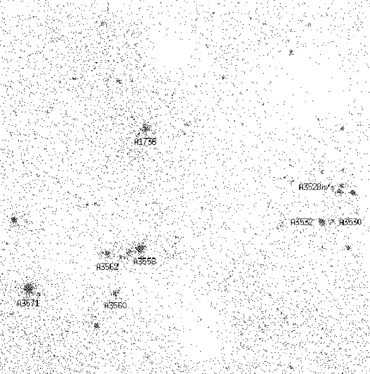
Figure 2.2: Raw RASS image of the Shapley supercluster with names of the main individual galaxy clusters overlaid. The box size is 13.8 deg. The apparent large scale variations of the background are caused by differences in the exposure time (find a better version of this image at www.reiprich.net).

Chapter 3 Sample

The mass function measures the cluster number density as a function of mass. Therefore any cluster fulfilling the selection criteria and not included in the sample distorts the result systematically. It is then obvious that for the construction of the mass function it is vital to use a homogeneously selected and highly complete sample of objects, and additionally the selection must be closely related to cluster mass. In this work the RASS, where one single instrument has surveyed the whole sky, has been chosen as the basis for the sample construction. Using the X-ray emission from the hot intracluster medium for cluster selection minimizes projection effects and the good correlation between X-ray luminosity and gravitational mass convincingly demonstrates that X-ray cluster surveys have the important property of being mass selective (Sect. 6.1).

Another aim of this work is the characterization of physical cluster properties. For such a statistical investigation it is important not to introduce any bias caused by selection effects. It is therefore desirable to select clusters by objective criteria, as performed here.

Several cluster catalogs have already been constructed from the RASS with high completeness down to low flux limits (see refs below). These have been utilized for the selection of candidates. Low thresholds have been set for the initial selection in order not to miss any cluster due to measurement uncertainties. These candidates have been homogeneously reanalyzed, using higher quality ROSAT PSPC pointed observations whenever possible (Chap. 4). A flux limit well above the limit for candidate selection has then been applied to define the new flux-limited sample of the brightest clusters in the sky.

In detail the candidates emerged from the following input catalogs. Table 3 lists the selection criteria and the number of clusters selected from each of the catalogs, that are contained in the final sample.

• The REFLEX (ROSAT-ESO Flux-Limited X-ray) galaxy cluster survey (Böhringer et al., 2001b ) covers the southern hemisphere (declination $\delta\leq$ +2.5 deg; galactic latitude $|b_{\rm II}|\geq 20.0$ deg) with a flux limit $f_{\rm X,lim}(0.1-2.4\,{\rm keV})=3.0\,\times 10^{-12}\,{\rm ergs\,s^{-1}\,cm^{-2}}$.

• The NORAS (Northern ROSAT All-Sky) galaxy cluster survey (Böhringer et al., 2000) contains clusters showing extended emission in the RASS in the northern hemisphere ($\delta\geq$ 0.0 deg; $|b_{\rm II}|\geq 20.0$ deg) with count rates $C_{\rm X}(0.1-2.4\,{\rm keV})\geq 0.06\,{\rm cts\,s^{-1}}$.

• NORAS II (J. Retzlaff et al., in prep.) is the continuation of the NORAS survey project. It includes point like sources and aims for a flux limit $f_{\rm X,lim}(0.1-2.4\,{\rm keV})=2.0\,\times 10^{-12}\,{\rm ergs\,s^{-1}\,cm^{-2}}$.

• The BCS (ROSAT Brightest Cluster Sample) (Ebeling et al., 1998) covers the northern hemisphere ($\delta\geq$ 0.0 deg; galactic latitude $|b_{\rm II}|\geq 20.0$ deg) with $f_{\rm X,lim}(0.1-2.4\,{\rm keV})=4.4\,\times 10^{-12}\,{\rm ergs\,s^{-1}\,cm^{-2}}$ and redshifts $z\leq 0.3$.

• The RASS 1 Bright Sample of Clusters of Galaxies (De Grandi et al., 1999) covers the south galactic cap region in the southern hemisphere ($\delta<$ +2.5 deg; $b_{\rm II}<-20.0$ deg) with an effective flux limit $f_{\rm X,lim}(0.5-2.0\,{\rm keV})$ between $\sim$ 3 and $4\,\times 10^{-12}\,{\rm ergs\,s^{-1}\,cm^{-2}}$.

• XBACs (X-ray Brightest Abell-type Clusters of galaxies) (Ebeling et al., 1996) is an all-sky sample of Abell, (1958)/ACO (Abell et al., 1989) clusters limited to high galactic latitudes $|b_{\rm II}|\geq 20.0$ deg with nominal ACO redshifts $z\leq 0.2$ and X-ray fluxes $f_{\rm X}(0.1-2.4\,{\rm keV})>5.0\,\times 10^{-12}\,{\rm ergs\,s^{-1}\,cm^{-2}}$.

• An all-sky list of Abell/ACO/ACO-supplementary clusters (H. Böhringer 1999, private communication) with count rates $C_{\rm X}(0.5-2.0\,{\rm keV})\geq 0.6\,{\rm cts\,s^{-1}}$.

• Early type galaxies with measured RASS count rates from a magnitude limited sample of Beuing et al., (1999) have been been checked in order not to miss any X-ray faint groups.

• All clusters from the sample of Lahav et al., (1989) and Edge et al., (1990), where clusters had been compiled from various X-ray missions, have been checked.

Table 3.1: Selection of candidates

Sample	$C_{\rm X}\ [{\rm cts\,s^{-1}}]$				$f_{\rm X}\ [10^{-11}\,{\rm ergs\,s^{-1}\,cm^{-2}}]$		$N_{\rm Cl}$	Ref.
	$0.1-2.4\,{\rm keV}$	$0.5-2.0\,{\rm keV}$	$0.64-2.36\,{\rm keV}$		$0.1-2.4\,{\rm keV}$	$0.5-2.0\,{\rm keV}$
REFLEX		0.9			1.7		33	1
NORAS		0.7			1.7		25	2
NORAS II		0.7			1.7		4	3
BCS	1.0				1.7		1	4
RASS 1						1.0	0	5
XBACs	1.0				1.7		0	6
Abell/ACO		0.7					0	7
early type			0.7				0	8
previous sat							0	9

Note. — Only one of the criteria, count rate or flux, has to be met for a cluster to be selected as candidate. The catalogs are listed in search sequence, therefore $N_{\rm Cl}$ gives the number of candidates additionally selected from the current catalog and contained in the final flux-limited sample. So in the case of NORAS a cluster is selected as candidate if it fulfils $C_{\rm X}(0.5-2.0\,{\rm keV})\geq 0.7\,{\rm cts\,s^{-1}}$ or $f_{\rm X}(0.1-2.4\,{\rm keV})\geq 1.7\times 10^{-11}\,{\rm ergs\,s^{-1}\,cm^{-2}}$ and has not already been selected from REFLEX. This candidate is counted under $N_{\rm Cl}$ if it meets the selection criteria for HIFLUGCS.

References. — (1) Böhringer et al., 2001b ; (2) Böhringer et al., 2000; (3) J. Retzlaff et al., in prep.; (4) Ebeling et al., 1998; (5) De Grandi et al., 1999; (6) Ebeling et al., 1996; (7) H. Böhringer 1999, private communication; (8) Beuing et al., 1999; (9) Lahav et al., 1989; Edge et al., 1990.

The main criterion for candidate selection, a flux threshold $1.7\times 10^{-11}\,{\rm ergs\,s^{-1}\,cm^{-2}}$, has been chosen to allow for measurement uncertainties. E.g., for REFLEX clusters with $1.5\times 10^{-11}\,{\rm ergs\,s^{-1}\,cm^{-2}}\leq f_{\rm X}\leq 2.5\times 10^{-11}\,{\rm ergs\,s^{-1}\,cm^{-2}}$ the mean statistical flux error is less than 8 %. With an additional mean systematic error of 6 %, caused by underestimation of fluxes due to the comparatively low RASS exposure times, the flux threshold of $1.7\times 10^{-11}\,{\rm ergs\,s^{-1}\,cm^{-2}}$ for candidate selection then ensures that no clusters are missed for a final flux limit $f_{\rm X,lim}=2.0\times 10^{-11}\,{\rm ergs\,s^{-1}\,cm^{-2}}$.

Almost none of the fluxes given in the input catalogs have been calculated using a measured X-ray temperature, but mostly using gas temperatures estimated from an $L_{\rm X}$–$T_{\rm X}$ relation. In order to be independent of this additional uncertainty clusters have also be selected as candidates if they exceed a count rate threshold which corresponds to $f_{\rm X}(0.1-2.4\,{\rm keV})=2.0\times 10^{-11}\,{\rm ergs\,s^{-1}\,cm^{-2}}$ for a typical cluster temperature, $T_{\rm gas}=4\,\rm keV$, and redshift, $z=0.05$, and for an exceptionally high neutral hydrogen column density, e.g., in the NORAS case $n_{\rm h}=1.6\,\times 10^{21}\rm cm^{-2}$.

Most of the samples mentioned above excluded the area on the sky close to the galactic plane as well as the area of the Magellanic Clouds. In order to construct a highly complete sample from the candidate list the following selection criteria that successful clusters must fulfil have been applied:

• redetermined flux $f_{\rm X}(0.1-2.4\,{\rm keV})\geq 2.0\times 10^{-11}\,{\rm ergs\,s^{-1}\,cm^{-2}}$,

• galactic latitude $|b_{\rm II}|\geq 20.0$ deg,

• projected position outside the excluded 324 deg² area of the Magellanic Clouds (see Tab. 3.2),

• projected position outside the excluded 98 deg² region of the Virgo galaxy cluster (see Tab. 3.2).

Table 3.2: Regions of the sky not sampled in HIFLUGCS

Region	RA Range	DEC Range	Area (sr)
LMC 1	58 $\to 103^{o}$	$-63\to-77^{o}$	0.0655
LMC 2	81 $\to 89^{o}$	$-58\to-63^{o}$	0.0060
LMC 3	103 $\to 108^{o}$	$-68\to-74^{o}$	0.0030
SMC 1	358.5 $\to 20^{o}$	$-67.5\to-77^{o}$	0.0189
SMC 2	356.5 $\to 358.5^{o}$	$-73\to-77^{o}$	0.0006
SMC 3	20 $\to 30^{o}$	$-67.5\to-72^{o}$	0.0047
Virgo	182.7 $\to 192.7^{o}$	$7.4\to 17.4^{o}$	0.0297
Milky Way	0 $\to 360^{o}$ ($l_{\rm II}$)	$-20\to 20^{o}$ ($b_{\rm II}$)	4.2980

Note. — Excised areas for the Magellanic Clouds are the same as in Böhringer et al., 2001b , because REFLEX forms the basic input catalog in the southern hemisphere.

These selection criteria are fulfilled by 63 candidates. The advantages of the redetermined fluxes over the fluxes from the input catalogs are summarized in Chap. 4. In Tab. 3 one notes that 98 % of all clusters in HIFLUGCS have been flagged as candidates in REFLEX, NORAS, or in the candidate list for NORAS II; these surveys are not only all based on the RASS but all use the same algorithm for the count rate determination, further substantiating the homogeneous candidate selection for HIFLUGCS.

The fraction of available ROSAT PSPC pointed observations for clusters included in HIFLUGCS equals 86 %. The actually used fraction is slightly reduced to 75 % because some clusters appear extended beyond the PSPC field of view and therefore RASS data had to be used. The fraction of clusters with published ASCA temperatures equals 87 %. If a lower flux limit had been chosen the fraction of available PSPC pointed observations and published ASCA temperatures would have been decreased thereby increasing the uncertainties in the derived cluster parameters. Furthermore this value for the flux limit ensures that no corrections, due to low exposure in the RASS or high galactic hydrogen column density, need to be applied for the effective area covered. This can be seen by the effective sky coverage in the REFLEX survey area: for a flux limit $f_{\rm X,lim}(0.1-2.4\,{\rm keV})=2.0\,\times 10^{-11}\,{\rm ergs\,s^{-1}\,cm^{-2}}$ and a minimum of 30 source counts the sky coverage amounts to 99 %. The clear advantage is that the HIFLUGCS catalog can be used in a straightforward manner in statistical analyses, because the effective area is the same for all clusters and simply equals the covered solid angle on the sky.

The distribution of clusters included in HIFLUGCS projected onto the sky is shown in Fig. 3.1. The sky coverage for the cluster sample equals 26 721.8 deg² (8.13994 sr), about two thirds of the sky. The cluster names, coordinates and redshifts are listed in Tab. 4.1. Further properties of the cluster sample and completeness tests are discussed in Sect. 7.

For later analyses which do not necessarily require a complete sample, e.g., correlations between physical parameters, 43 clusters (not included in HIFLUGCS) from the candidate list have been combined with HIFLUGCS to form an ‘extended sample’ of 106 clusters. This sample is not a purely flux-limited sample with clearly defined selection criteria. Nevertheless this extended sample is not dominated by subjective selection and therefore one may take advantage of the increased statistics. The difference between the results of relations using HIFLUGCS and the extended sample is discussed in Sect. 6.1.

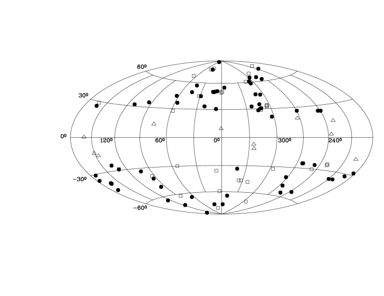
Figure 3.1: Aitoff projection of the 63 HIFLUGCS galaxy clusters in galactic coordinates (filled circles). Additionally shown are 11 clusters above the flux limit but with $|b_{\rm II}|<20.0\,\rm deg$ (open triangles) and 32 clusters with fluxes below the flux limit (open squares).

Chapter 4 Reduction and Analysis

This Chapter describes the derivation of the basic quantities in this work, e.g., count rates, fluxes, luminosities, and mass estimates for the galaxy clusters. These and other relevant cluster parameters are tabulated along with their uncertainties.

4.1 Flux Determination

Measuring the count rate of galaxy clusters is an important step in constructing a flux-limited cluster sample. The count rate determination performed here is based on the growth curve analysis method (Böhringer et al., 2000), with modifications adapted to the higher photon statistics available here. The main features of the method as well as the modifications are outlined below.

The instrument used is the ROSAT PSPC (Pfeffermann et al., 1987), with a low internal background ideally suited for this study which needs good signal to noise of the outer, low surface brightness regions of the clusters. Mainly pointed observations from the public archive at MPE have been used. If the cluster is extended beyond the PSPC field of view making a proper background determination difficult or if there is no pointed PSPC observation available, RASS data have been used. The ROSAT hard energy band (channels $52-201\approx 0.5-2.0\,{\rm keV}$) has been used for all count rate measurements because of the higher background in the soft band. The reduction of the soft X-ray background is about a factor of four in the hard band, while still 60–100 % of the cluster emission is detected (Böhringer et al., 2000). Therefore the signal to noise ratio is multiplied by a factor 0.92–1.25 if the hard band is used.

Two X-ray cluster centers are determined by finding the two-dimensional ‘center of mass’ of the photon distribution iteratively for an aperture radius of 3 and 7.5 arcmin around the starting position. The small aperture yields the center representing the position of the cluster’s peak emission and therefore probably indicates the position where the cluster’s potential well is deepest. This center is used for the regional selection, e.g. $|b_{\rm II}|\geq 20.0$. The more globally defined center with the larger aperture is used for the subsequent analysis tasks since for the mass determination it is most important to have a good estimate of the slope of the surface brightness profile in the outer parts of the cluster.

The background surface brightness is determined in a ring outside the cluster emission. To minimize the influence of discrete sources the ring is subdivided into twelve parts of equal area and a sigma clipping is performed. To determine the count rate the area around the global center is divided into concentric rings. For pointed observations 200 rings with a width of 15 arcsec each are used. Due to the lower photon statistics a width of 30 arcsec is used for RASS data and the number of rings depends on the field size extracted ($100-300$ rings for field sizes of $2\times 2\,\rm deg^{2}-8\times 8\,\rm deg^{2}$). Each photon is divided by the vignetting and deadtime corrected exposure time of the skypixel where it has been detected and these ratios are summed up in each ring yielding the ring count rate. From this value the background count rate for the respective ring area is subtracted yielding a source ring count rate. These individual source ring count rates are integrated with increasing radius yielding the (cumulative) source count rate for a given radius (Fig. 4.1). Obvious contaminating point sources have been excluded manually. The cut-out regions have then been assigned the average surface brightness of the ring. If a cluster has been found to be clearly made up of two major components, for instance A3395n/s, these components have been treated separately. This procedure ensures that double clusters are not treated as a single entity for which spherical symmetry is assumed. For the same reason strong subtructure has been excluded in the same manner as contaminating point sources. In this work the aim is to characterize all cluster properties consistently and homogeneously. Therefore if strong substructure is identified then it is excluded for the flux/luminosity and mass determination.

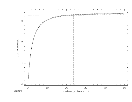
Figure 4.1: Cumulative source count rate as a function of radius (solid line) for the cluster A2029 (pointed observation). The vertical dashed line indicates the outer significance radius, $r_{\rm X}$. The dashed lines just above and below the source count rate indicate the 1-$\sigma$ Poissonian errors.

An outer significance radius of the cluster, $r_{\rm X}$, is determined at the position from where on the Poissonian 1-$\sigma$ error rises faster than the source count rate. Usually the source count rate settles into a nearly horizontal line for radii larger than $r_{\rm X}$. In some cases, however, the source count rate seems to increase or decrease roughly quadratically for radii larger than $r_{\rm X}$ indicating a possibly under- or overestimated background (Fig. 4.2). Therefore a parabola of the form $y=mx^{2}+b$ has been fitted to the source count rate for radii larger than $r_{\rm X}$ and the measured background has been corrected. An example for a corrected source count rate profile is shown in Fig. 4.3.

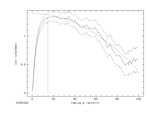
Figure 4.2: Cumulative source count rate as a function of radius for the cluster EXO0422, shown as an extreme example (RASS data). The parabolic dashed line indicates the best fit parabola for count rates larger than $r_{\rm X}$.

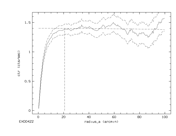
Figure 4.3: Corrected cumulative source count rate as a function of radius for the cluster EXO0422. The count rate correction is less than 5 %.

Figure 4.4 shows for the extended sample (106 clusters) that the difference between measured and corrected source count rate is generally very small. Nevertheless an inspection of each count rate profile has been performed, to decide whether the measured or corrected count rate is adopted as the final count rate, to avoid artificial corrections due to large scale variations of the background (especially in the large RASS fields). The count rates are given in Tab. 4.1.

Figure 4.4: Comparison of measured and corrected source count rates for the extended sample of 106 galaxy clusters. The solid line indicates equality.

The conversion factor for the count rate to flux conversion depends on the hydrogen column density, $n_{\rm h}$, on the cluster gas temperature, $T_{\rm gas}$, on the cluster gas metallicity, $A$, on the cluster redshift, $z$, and on the respective detector responses for the two different PSPCs used. The $n_{\rm h}$ value is taken as the value inferred from 21 cm radio measurements for our galaxy at the projected cluster position (Dickey and Lockman, 1990; included in the EXSAS software package, Zimmermann et al., 1998; photoelectric absorption cross sections are taken from Morrison and McCammon, 1983). Gas temperatures have been estimated by compiling X-ray temperatures, $T_{\rm X}$, from the literature, giving preference to temperatures measured with the ASCA satellite. For clusters where no ASCA measured temperature has been available, $T_{\rm X}$ measured with previous X-ray satellites have been used. The X-ray temperatures and corresponding references are given in Tab. 4.2. For two clusters included in HIFLUGCS no measured temperature has been found in the literature and the $L_{\rm X}(<2\,h_{50}^{-1}\,{\rm Mpc})-T_{\rm X}$ relation of Markevitch, (1998) has been used. The relation for non cooling flow corrected luminosities and cooling flow corrected/emission weighted temperatures has been chosen, because the luminosities determined here have not been corrected for cooling flows and cooling flow corrected temperatures should be a better estimate of the cluster virial temperature. For $h_{50}=1$ this relation reads

$$T_{\rm X}=\left[{\frac{L_{\rm X}(<2\,\rm Mpc)}{6.28\times 10^{44}\,{\rm ergs\,s^{-1}}}}\right]^{1/2.09}\times 6\rm\,keV\,.$$ (4.1)

Since the conversion from count rate to flux depends only weakly on $T_{\rm gas}$ in the ROSAT energy band for the relevant temperature range a cluster temperature $k_{\rm B}T_{\rm gas}=4\,{\rm keV}$ has been assumed in a first step to determine $L_{\rm X}(<2\,h_{50}^{-1}\,{\rm Mpc})$ for the clusters where no gas temperature has been found in the literature. With this luminosity the gas temperature has been estimated. The metallicity is set to 0.35 times the solar value for all clusters (e.g., Arnaud et al., 1992, see also Chap. 5). The redshifts have been compiled from the literature and are given in Tab. 4.1 together with the corresponding references. With these quantities and the count rates given in Tab. 4.1 fluxes in the observer rest frame energy range $0.1-2.4\,{\rm keV}$ have been calculated applying a modern version of a Raymond–Smith spectral code (Raymond and Smith, 1977). The results are listed in Tab. 4.1. The flux calculation has also been checked using XSPEC (Arnaud, 1996) by folding the model spectrum created with the parameters given above with the detector response and adjusting the normalization to reproduce the observed count rate. It is found that for 90 % of the clusters the deviation between the two results for the flux measurement is less than 1 %. Luminosities in the source rest frame energy range $0.1-2.4\,{\rm keV}$ have then been calculated within XSPEC by adjusting the normalization to reproduce the initial flux measurements.

The improvements of the flux determination performed here compared to the input catalogs in general are now summarized.

• Due to the use of a high fraction of pointed observations the photon statistics is on average much better, e.g, for the 33 clusters contained in REFLEX and HIFLUGCS one finds a mean of 841 and 19580 source photons, respectively. Consequently the cluster emission has been traced out to larger radii for HIFLUGCS.

• The higher photon statistics has allowed a proper exclusion of contaminating point sources (stars, active galactic nuclei (AGN), etc.) and substructure, and the separation of double clusters.

• An iterative background correction has been performed.

• A measured X-ray temperature is used for the flux determination in most cases.

Simulations have shown that even for the HIFLUGCS clusters with the lowest number of photons the determined flux shows no significant trend with redshift in the relevant redshift range (Ikebe et al., 2001).

The parameters of the table columns of Tab. 4.1 are described as follows. Column (1) lists the cluster name. Names have been truncated to at most eight characters. Columns (2) and (3) give the equatorial coordinates of the cluster center used for the regional selection for the epoch J2000 in decimal degrees. Column (4) gives the heliocentric cluster redshift. Column (5) lists the column density of neutral galactic hydrogen in units of $10^{20}\,\rm atoms\,cm^{-2}$. Column (6) gives the count rate in the channel range 52–201 which corresponds to about (the energy resolution of the PSPC is limited) the energy range $0.5-2.0\,{\rm keV}$ in units of ${\rm cts\,s^{-1}}$. Column (7) lists the relative ($1-\sigma$ Poissonian) error of the count rate, the flux, and the luminosity in percent. Column (8) gives the significance radius in $h_{50}^{-1}\,{\rm Mpc}$. Column (9) lists the flux in the energy range $0.1-2.4\,{\rm keV}$ in units of $10^{-11}\,{\rm ergs\,s^{-1}\,cm^{-2}}$. Column (10) gives the luminosity in the energy range $0.1-2.4\,{\rm keV}$ in units of $h_{50}^{-2}\,10^{44}\,{\rm ergs\,s^{-1}}$. Column (11) gives the bolometric luminosity (energy range $0.01-40\,{\rm keV}$) in units of $h_{50}^{-2}\,10^{44}\,{\rm ergs\,s^{-1}}$. Column (12) indicates whether a RASS (R) or a pointed (P) ROSAT PSPC observation has been used. Column (13) lists the code for the redshift reference decoded at the end of the table.

Table 4.1: Cluster properties

Cluster	R.A.	Dec.	$z$	$n_{\rm h}$	$C_{\rm X}$	$\Delta$	$r_{\rm X}$	$f_{\rm X}$	$L_{\rm X}$	$L_{\rm Bol}$	Obs	Ref
(1)	(2)	(3)	(4)	(5)	(6)	(7)	(8)	(9)	(10)	(11)	(12)	(13)
A0085	10.4632	$-9.3054$	0.0556	3.58	3.488	0.6	2.13	7.429	9.789	24.448	P	2
A0119	14.0649	$-1.2489$	0.0440	3.10	1.931	0.9	2.68	4.054	3.354	7.475	P	1
A0133	15.6736	$-21.8806$	0.0569	1.60	1.058	0.8	1.52	2.121	2.944	5.389	P	3
NGC507	20.9106	$33.2553$	0.0165	5.25	1.093	1.3	0.88	2.112	0.247	0.326	P	5
A0262	28.1953	$36.1528$	0.0161	5.52	4.366	3.8	1.48	9.348	1.040	1.533	R	6
A0400	44.4152	$6.0170$	0.0240	9.38	1.146	1.1	1.85	2.778	0.686	1.033	P	8
A0399	44.4684	$13.0462$	0.0715	10.58	1.306	5.4	3.18	3.249	7.070	17.803	R	6
A0401	44.7384	$13.5796$	0.0748	10.19	2.104	1.1	3.81	5.281	12.553	34.073	P	6
A3112	49.4912	$-44.2367$	0.0750	2.53	1.502	1.1	2.18	3.103	7.456	16.128	P	1
FORNAX	54.6686	$-35.3103$	0.0046	1.45	5.324	5.6	0.53	9.020	0.082	0.107	P+R	4
2A0335	54.6690	$9.9713$	0.0349	18.64	3.028	0.8	1.54	9.162	4.789	7.918	P	10
IIIZw54	55.3225	$15.4076$	0.0311	16.68	0.708	7.7	1.27	2.001	0.831	1.226	R	11
A3158	55.7282	$-53.6301$	0.0590	1.06	1.909	1.5	1.94	3.794	5.638	12.779	P	1
A0478	63.3554	$10.4661$	0.0900	15.27	1.827	0.6	3.12	5.151	17.690	49.335	P	6
NGC1550	64.9066	$2.4151$	0.0123	11.59	1.979	5.4	0.71	4.632	0.302	0.407	R	13
EXO0422	66.4637	$-8.5581$	0.0390	6.40	1.390	6.2	1.32	3.085	2.015	3.283	R	10
A3266	67.8410	$-61.4403$	0.0594	1.48	2.879	0.7	2.99	5.807	8.718	23.663	P	4
A0496	68.4091	$-13.2605$	0.0328	5.68	3.724	0.7	1.78	8.326	3.837	7.306	P	8
A3376	90.4835	$-39.9741$	0.0455	5.01	1.115	1.4	2.86	2.450	2.174	4.077	P	4
A3391	96.5925	$-53.6938$	0.0531	5.42	0.999	1.9	1.98	2.225	2.681	5.857	P	4
A3395s	96.6920	$-54.5453$	0.0498	8.49	0.836	3.8	1.45	2.009	2.131	4.471	P	4
A0576	110.3571	$55.7639$	0.0381	5.69	1.374	6.8	2.32	3.010	1.872	3.518	R	6
A0754	137.3338	$-9.6797$	0.0528	4.59	1.537	1.6	1.91	3.366	3.990	11.967	P	6
HYDRA-A	139.5239	$-12.0942$	0.0538	4.86	2.179	0.6	1.66	4.776	5.930	11.520	P	13
A1060	159.1784	$-27.5212$	0.0114	4.92	4.653	3.3	0.95	9.951	0.554	0.945	R	6
A1367	176.1903	$19.7030$	0.0216	2.55	2.947	0.8	1.55	6.051	1.206	2.140	P	8
MKW4	181.1124	$1.8962$	0.0200	1.86	1.173	1.7	1.23	2.268	0.390	0.543	P	10
ZwCl1215	184.4220	$3.6604$	0.0750	1.64	1.081	1.3	2.55	2.183	5.240	11.656	P	19
NGC4636	190.7084	$2.6880$	0.0037	1.75	3.102	7.2	0.39	4.085	0.023	0.027	R	13
A3526	192.1995	$-41.3087$	0.0103	8.25	11.655	2.2	1.64	27.189	1.241	2.238	R	15
A1644	194.2900	$-17.4029$	0.0474	5.33	1.853	5.1	1.85	4.030	3.876	7.882	R	8
A1650	194.6712	$-1.7572$	0.0845	1.54	1.218	6.6	3.17	2.405	7.308	17.955	R	6
A1651	194.8419	$-4.1947$	0.0860	1.71	1.254	1.2	2.03	2.539	8.000	18.692	P	22
COMA	194.9468	$27.9388$	0.0232	0.89	17.721	1.4	4.04	34.438	7.917	22.048	R	8
NGC5044	198.8530	$-16.3879$	0.0090	4.91	3.163	0.5	0.56	5.514	0.193	0.246	P	24
A1736	201.7238	$-27.1765$	0.0461	5.36	1.631	6.3	2.47	3.537	3.223	5.682	R	25
A3558	201.9921	$-31.5017$	0.0480	3.63	3.158	0.5	2.11	6.720	6.615	14.600	P	1
A3562	203.3984	$-31.6678$	0.0499	3.91	1.367	0.9	2.01	2.928	3.117	6.647	P	4
A3571	206.8692	$-32.8553$	0.0397	3.93	5.626	0.7	2.35	12.089	8.132	20.310	P	21
A1795	207.2201	$26.5944$	0.0616	1.20	3.132	0.3	2.14	6.270	10.124	27.106	P	6
A3581	211.8852	$-27.0153$	0.0214	4.26	1.603	3.2	0.64	3.337	0.657	0.926	P	28
MKW8	220.1596	$3.4717$	0.0270	2.60	1.255	8.4	1.90	2.525	0.789	1.355	R	29
A2029	227.7331	$5.7450$	0.0767	3.07	3.294	0.6	2.78	6.938	17.313	50.583	P	6
A2052	229.1846	$7.0211$	0.0348	2.90	2.279	1.0	1.14	4.713	2.449	4.061	P	6
MKW3S	230.4643	$7.7059$	0.0450	3.15	1.578	1.0	1.39	3.299	2.865	5.180	P	10
A2065	230.6096	$27.7120$	0.0721	2.84	1.227	6.1	3.09	2.505	5.560	12.271	R	6
A2063	230.7734	$8.6112$	0.0354	2.92	2.038	1.3	2.13	4.232	2.272	4.099	P	8
A2142	239.5824	$27.2336$	0.0899	4.05	2.888	0.9	3.09	6.241	21.345	64.760	P	6
A2147	240.5628	$15.9586$	0.0351	3.29	2.623	3.2	1.87	5.522	2.919	6.067	P	8
A2163	243.9433	$-6.1436$	0.2010	12.27	0.773	1.5	3.15	2.039	34.128	123.200	P	31
A2199	247.1586	$39.5477$	0.0302	0.84	5.535	1.8	2.37	10.642	4.165	7.904	R	8
A2204	248.1962	$5.5733$	0.1523	5.94	1.211	1.6	3.29	2.750	26.938	68.989	P	6
A2244	255.6749	$34.0578$	0.0970	2.07	1.034	2.1	2.64	2.122	8.468	21.498	P	6
A2256	255.9884	$78.6481$	0.0601	4.02	2.811	1.4	3.09	6.054	9.322	22.713	P	6
A2255	258.1916	$64.0640$	0.0800	2.51	0.976	1.2	3.22	2.022	5.506	13.718	P	6
A3667	303.1362	$-56.8419$	0.0560	4.59	3.293	0.7	2.81	7.201	9.624	24.233	P	1
S1101	348.4941	$-42.7268$	0.0580	1.85	1.237	0.9	1.64	2.485	3.597	5.939	P	35
A2589	350.9868	$16.7753$	0.0416	4.39	1.200	1.3	1.46	2.591	1.924	3.479	P	37
A2597	351.3318	$-12.1246$	0.0852	2.50	1.074	1.2	1.43	2.213	6.882	13.526	P	6
A2634	354.6201	$27.0269$	0.0312	5.17	1.096	1.6	1.79	2.415	1.008	1.822	P	6
A2657	356.2334	$9.1952$	0.0404	5.27	1.148	0.9	1.52	2.535	1.771	3.202	P	8
A4038	356.9322	$-28.1415$	0.0283	1.55	2.854	1.3	1.35	5.694	1.956	3.295	P	4
A4059	359.2541	$-34.7591$	0.0460	1.10	1.599	1.3	1.72	3.170	2.872	5.645	P	36
Clusters from the extended sample not included in HIFLUGCS.
A2734	2.8389	$-28.8539$	0.0620	1.84	0.710	2.5	1.74	1.434	2.365	4.357	P	1
A2877	17.4796	$-45.9225$	0.0241	2.10	0.801	1.2	1.06	1.626	0.405	0.714	P	4
NGC499	20.7971	$33.4587$	0.0147	5.25	0.313	2.5	0.30	0.479	0.045	0.051	P	5
AWM7	43.6229	$41.5781$	0.0172	9.21	7.007	2.0	1.58	16.751	2.133	3.882	R	7
PERSEUS	49.9455	$41.5150$	0.0183	15.69	40.723	0.8	3.30	113.731	16.286	40.310	R	9
S405	58.0078	$-82.2315$	0.0613	7.65	0.781	8.2	2.14	1.800	2.899	5.574	R	12
3C129	72.5602	$45.0256$	0.0223	67.89	1.512	5.6	1.61	10.566	2.242	4.996	R	10
A0539	79.1560	$6.4421$	0.0288	12.06	1.221	1.3	1.37	3.182	1.135	1.935	P	14
S540	85.0265	$-40.8431$	0.0358	3.53	0.788	5.0	0.84	1.611	0.887	1.353	R	4
A0548w	86.3785	$-25.9340$	0.0424	1.79	0.136	5.4	0.73	0.234	0.183	0.240	P	15
A0548e	87.1596	$-25.4692$	0.0410	1.88	0.771	1.8	2.12	1.551	1.117	1.870	P	15
A3395n	96.9005	$-54.4447$	0.0498	5.42	0.699	3.9	1.37	1.555	1.650	3.461	P	4
UGC03957	115.2481	$55.4319$	0.0340	4.59	0.936	6.0	0.94	1.975	0.980	1.531	R	16
PKS0745	116.8837	$-19.2955$	0.1028	43.49	1.268	1.0	2.44	6.155	27.565	70.604	P	17
A0644	124.3553	$-7.5159$	0.0704	5.14	1.799	1.0	4.02	3.994	8.414	22.684	P	6
S636	157.5151	$-35.3093$	0.0116	6.42	3.102	4.9	1.18	5.869	0.341	0.446	R	18
A1413	178.8271	$23.4051$	0.1427	1.62	0.636	1.6	2.39	1.289	11.090	28.655	P	6
M49	187.4437	$7.9956$	0.0044	1.59	1.259	1.0	0.27	1.851	0.015	0.019	P	15
A3528n	193.5906	$-29.0130$	0.0540	6.10	0.560	2.3	1.51	1.263	1.581	2.752	P	1
A3528s	193.6708	$-29.2254$	0.0551	6.10	0.756	1.6	1.35	1.703	2.224	3.746	P	20
A3530	193.9211	$-30.3451$	0.0544	6.00	0.438	2.8	1.55	0.987	1.252	2.317	P	21
A3532	194.3375	$-30.3698$	0.0539	5.96	0.797	1.8	1.64	1.797	2.235	4.483	P	21
A1689	197.8726	$-1.3408$	0.1840	1.80	0.712	1.1	2.36	1.454	20.605	60.707	P	23
A3560	203.1119	$-33.1355$	0.0495	3.92	0.714	2.5	2.00	1.519	1.601	2.701	P	26
A1775	205.4582	$26.3820$	0.0757	1.00	0.654	1.8	2.02	1.290	3.175	5.735	P	27
A1800	207.3408	$28.1038$	0.0748	1.18	0.610	7.9	1.98	1.183	2.840	5.337	R	28
A1914	216.5035	$37.8268$	0.1712	0.97	0.729	1.4	2.35	1.454	17.813	56.533	P	6
NGC5813	225.2994	$1.6981$	0.0064	4.19	0.976	6.7	0.17	1.447	0.025	0.029	R	13
NGC5846	226.6253	$1.6089$	0.0061	4.25	0.569	2.3	0.21	0.851	0.014	0.016	P	13
A2151w	241.1465	$17.7252$	0.0369	3.36	0.754	1.9	1.46	1.568	0.917	1.397	P	8
A3627	243.5546	$-60.8430$	0.0163	20.83	9.962	3.0	2.20	31.084	3.524	8.179	R	30
TRIANGUL	249.5758	$-64.3557$	0.0510	12.29	4.294	0.7	2.54	11.308	12.508	37.739	P	32
OPHIUCHU	258.1115	$-23.3634$	0.0280	20.14	11.642	2.0	2.29	35.749	11.953	37.391	R	33
ZwCl1742	266.0623	$32.9893$	0.0757	3.56	0.889	4.4	1.83	1.850	4.529	9.727	R	34
A2319	290.2980	$43.9484$	0.0564	8.77	5.029	1.0	3.57	12.202	16.508	47.286	P	6
A3695	308.6991	$-35.8135$	0.0890	3.56	0.836	9.2	2.58	1.739	5.882	12.715	R	1
IIZw108	318.4752	$2.5564$	0.0494	6.63	0.841	7.3	2.20	1.884	1.969	3.445	R	5
A3822	328.5438	$-57.8668$	0.0760	2.12	0.964	7.3	3.18	1.926	4.758	9.877	R	1
A3827	330.4869	$-59.9641$	0.0980	2.84	0.953	5.8	1.78	1.955	7.963	20.188	R	1
A3888	338.6255	$-37.7343$	0.1510	1.20	0.546	2.4	1.52	1.096	10.512	30.183	P	23
A3921	342.5019	$-64.4286$	0.0936	2.80	0.626	1.7	2.43	1.308	4.882	11.023	P	12
HCG94	349.3041	$18.7060$	0.0417	4.55	0.820	1.0	2.09	1.775	1.324	2.319	P	36
RXJ2344	356.0723	$-4.3776$	0.0786	3.54	0.653	1.4	1.61	1.385	3.661	7.465	P	12

Note. — The columns are described in detail at the end of Section 4.1.

References. — (1) Katgert et al., 1996. (2) Mazure et al., 1996. (3) Median of 9 galaxy redshifts compiled from Lauberts and Valentijn, 1989; Merrifield and Kent, 1991; Loveday et al., 1996; Way et al., 1998. (4) Abell et al., 1989. (5) Huchra et al., 1999. (6) Struble and Rood, 1987. (7) dell’Antonio et al., 1994. (8) Zabludoff et al., 1993. (9) Poulain et al., 1992. (10) NED Team, 1992. (11) Böhringer et al., 2000. (12) De Grandi et al., 1999. (13) de Vaucouleurs et al., 1991. (14) Zabludoff et al., 1990. (15) den Hartog and Katgert, 1996. (16) Michel and Huchra, 1988. (17) Yan and Cohen, 1995. (18) Garcia, 1995. (19) Ebeling et al., 1998. (20) Median of 8 galaxy redshifts compiled from de Vaucouleurs et al., 1991; Quintana et al., 1995; Katgert et al., 1998. (21) Vettolani et al., 1990. (22) Allen et al., 1992. (23) Teague et al., 1990. (24) da Costa et al., 1998. (25) Dressler and Shectman, 1988. (26) Melnick and Moles, 1987. (27) Median of 13 galaxy redshifts compiled from Kirshner et al., 1983; Zabludoff et al., 1990; NED Team, 1992; Davoust and Considere, 1995; Oegerle et al., 1995. (28) Postman et al., 1992. (29) Andersen and Owen, 1994. (30) Kraan-Korteweg et al., 1996. (31) Elbaz et al., 1995. (32) Edge and Stewart, 1991a . (33) Lahav et al., 1989. (34) Ulrich, 1976. (35) Stocke et al., 1991. (36) Hickson et al., 1992. (37) Beers et al., 1991.

4.2 Mass Determination

The gravitational mass has been determined as outlined in Sect. 2.1.3 utilizing the surface brightness profile (Sect. 2.1.2.1) and the gas temperature (Sects. 2.1.2.2, 4.1). Since the general cluster temperature structure for radii larger than about half the virial radius has not been studied well observationally until now, isothermality is assumed. The influence of the isothermal assumption on the results is discussed in Chap. 7.

Having determined the integrated mass as a function of radius using (2.16), a physically meaningful fiducial radius for the mass measurement has to be defined. The radii commonly used are either the Abell radius, $r_{200}$, or $r_{500}$. The Abell radius is fixed at $r_{\rm A}\equiv 3\,h_{50}^{-1}\,{\rm Mpc}$. The radius $r_{200}$ ($r_{500}$) is the radius within which the mean gravitational mass density is equal to a multiple of the critical density of the universe, $\langle\rho_{\rm tot}\rangle=200\,(500)\,\rho_{\rm c}$. It has been shown that a correction for redshift is not necessary for the nearby clusters included in HIFLUGCS (Finoguenov et al., 2001) and the zero redshift value for $\rho_{\rm c}$ (see Eqs. 2.32, 2.40) is used for all calculations, i.e. $\rho_{\rm c}=4.6975\times 10^{-30}\rm g\,cm^{-3}$, unless noted otherwise. In Sect. 7.6.2 it is shown that the results are not affected if instead the cluster redshift is incorporated and a strong evolution model is assumed.

In order to treat clusters of different size in a homogeneous way the cluster mass is determined at a characteristic density but also the mass determined formally at a fixed radius is given for comparison. Spherical collapse models predict a virial density $\langle\rho_{\rm vir}\rangle\approx 178\,\rho_{\rm c}$ for $\Omega_{\rm m}=1$ (e.g., Kitayama and Suto, 1996), so a pragmatic approximation to the virial mass is to use $r_{200}$ as the outer boundary. Simulations performed by Evrard et al., (1996) have shown, however, that isothermal X-ray mass measurements may be biased towards high masses for $r>r_{500}$. Furthermore for most of the clusters in HIFLUGCS (86 %) up to $r_{500}$ no extrapolation outside the significantly detected cluster emission is necessary, i.e. $r_{500}<r_{\rm X}$, whereas the fraction is lower for $r_{200}$ (25 %) and $r_{\rm A}$ (17 %). In summary the most accurate results are expected for $M_{\rm tot}(<r_{500})\equiv M_{500}$, but for a comparison to predicted mass functions $M_{200}$ is the more appropriate value (see Sect. 2.2.3.2). Results for all determined masses and their corresponding radii are given in Tab. 4.2.

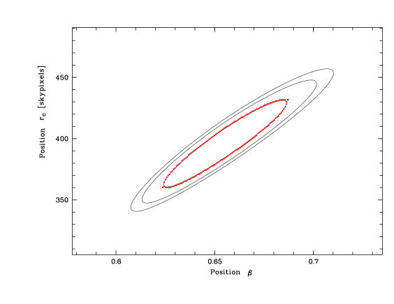
Figure 4.5: Confidence contours of the fit parameters $r_{\rm c}$ and $\beta$ for the cluster A3532 as a typical example. Shown are the 68, 90, and 95 % confidence levels (for two interesting parameters). The points on the 68 % error ellipse mark the value pairs used for the calculation of the uncertainty of the mass determination.

A major source of uncertainty comes from the temperature measurements. However, this (statistical) error is less than 5 % for one third of the clusters, therefore also other sources of error have to be taken into account, in particular one cannot neglect the uncertainties of the fit parameter values when assessing the statistical errors of the mass measurements. Therefore mass errors have been calculated by varying the fit parameter values, $\beta$ and $r_{\rm c}$, along their 68 % confidence level error ellipse (Fig. 4.5) and using the upper and lower bound of the quoted temperature ranges. The statistical mass error range has then been defined between the maximum and minimum mass. Note that a simple error propagation applied to (2.16) would underestimate the uncertainty on $M_{200}$ and $M_{500}$, since $r_{200}$ and $r_{500}$ also depend on $T_{\rm gas}$, $\beta$, and (weakly) $r_{\rm c}$. The individual mass errors have been used in subsequent calculations, unless noted otherwise. In log space errors in general have been transformed as $\Delta\log(x)=\log(e)\,(x^{+}-x^{-})/(2\,x)$, where $x^{+}$ and $x^{-}$ denote the upper and lower boundary of the quantity’s error range, respectively. A mean statistical error in the gravitational mass estimate of 23 % for clusters included in HIFLUGCS and a mean error of 27 % for the extended sample has been found.

The parameters of the table columns of Tab. 4.2 are described as follows. Column (1) lists the cluster name. Column (2) gives the $\beta$ parameter value and the corresponding 68 % c.l. statistical uncertainty for two interesting parameters. Column (3) gives the core radius in $h_{50}^{-1}\,{\rm kpc}$ and the corresponding uncertainty. Column (4) lists the X-ray temperature along with its error. Columns (5) and (7) give $M_{500}$ and $M_{200}$ and their uncertainties in units of $10^{14}\,h_{50}^{-1}\,M_{\odot}$. Columns (6) and (8) list $r_{500}$ and $r_{200}$ and their uncertainties in $h_{50}^{-1}\,{\rm Mpc}$. Column (9) gives $M_{\rm A}\equiv M_{\rm tot}(<r_{\rm A})$ in units of $10^{14}\,h_{50}^{-1}\,M_{\odot}$. Column (10) lists the code for the temperature reference decoded at the end of the table. Temperatures for codes 1–7 have been determined with ASCA, code 8 with ROSAT, code 9 with EXOSAT, code 10 with Einstein, and code 11 with a ROSAT–ASCA $L_{\rm X}$–$T_{\rm X}$ relation. Temperatures for code 11 are enclosed in parentheses and the corresponding errors have been calculated using the scatter in the $L_{\rm X}$–$T_{\rm X}$ relation.

In the following the parameters of the columns of Tab. 4.3 are described. Column (1) lists the cluster name. Column (2) gives the central gas density in units of $10^{-25}\,\rm g\,cm^{-3}$. In column (3) and (4) the gas masses are given in units of $10^{13}\,h_{50}^{-5/2}\,M_{\odot}$. The errors include the uncertainty of $r_{500}$ and $r_{200}$. The respective gas mass fractions ($f_{\rm gas}\equiv M_{\rm gas}M_{\rm tot}^{-1}$) are listed in columns (5) and (6). The errors are determined from the (symmetrized) uncertainty of $M_{\rm tot}$.

Table 4.2: Cluster properties

Cluster	$\beta$	$r_{\rm c}$	$T_{\rm X}$	$M_{500}$	$r_{500}$	$M_{200}$	$r_{200}$	$M_{\rm A}$	Ref
(1)	(2)	(3)	(4)	(5)	(6)	(7)	(8)	(9)	(10)
A0085	$0.532^{+0.004}_{-0.004}$	$83^{+3}_{-3}$	$6.90^{+0.40}_{-0.40}$	$6.84^{+0.66}_{-0.66}$	$1.68^{+0.05}_{-0.06}$	$10.80^{+1.12}_{-1.04}$	$2.66^{+0.09}_{-0.09}$	12.21	1
A0119	$0.675^{+0.026}_{-0.023}$	$501^{+28}_{-26}$	$5.60^{+0.30}_{-0.30}$	$6.23^{+0.92}_{-0.76}$	$1.63^{+0.08}_{-0.07}$	$10.76^{+1.50}_{-1.39}$	$2.66^{+0.11}_{-0.13}$	12.24	1
A0133	$0.530^{+0.004}_{-0.004}$	$45^{+2}_{-2}$	$3.80^{+2.00}_{-0.90}$	$2.78^{+2.51}_{-0.95}$	$1.24^{+0.30}_{-0.16}$	$4.41^{+4.00}_{-1.52}$	$1.97^{+0.47}_{-0.27}$	6.71	9
NGC507	$0.444^{+0.005}_{-0.005}$	$19^{+1}_{-1}$	$1.26^{+0.07}_{-0.07}$	$0.41^{+0.04}_{-0.04}$	$0.66^{+0.02}_{-0.02}$	$0.64^{+0.07}_{-0.06}$	$1.04^{+0.04}_{-0.04}$	1.86	2
A0262	$0.443^{+0.018}_{-0.017}$	$42^{+12}_{-10}$	$2.15^{+0.06}_{-0.06}$	$0.90^{+0.10}_{-0.09}$	$0.86^{+0.03}_{-0.03}$	$1.42^{+0.15}_{-0.13}$	$1.35^{+0.05}_{-0.04}$	3.17	2
A0400	$0.534^{+0.014}_{-0.013}$	$154^{+9}_{-9}$	$2.31^{+0.14}_{-0.14}$	$1.28^{+0.17}_{-0.15}$	$0.96^{+0.04}_{-0.04}$	$2.07^{+0.30}_{-0.25}$	$1.53^{+0.08}_{-0.06}$	4.10	2
A0399	$0.713^{+0.137}_{-0.095}$	$450^{+132}_{-100}$	$7.00^{+0.40}_{-0.40}$	$10.00^{+3.73}_{-2.48}$	$1.91^{+0.21}_{-0.18}$	$16.64^{+6.61}_{-4.32}$	$3.07^{+0.36}_{-0.30}$	16.24	1
A0401	$0.613^{+0.010}_{-0.010}$	$246^{+11}_{-10}$	$8.00^{+0.40}_{-0.40}$	$10.27^{+1.08}_{-0.93}$	$1.92^{+0.07}_{-0.05}$	$16.59^{+1.62}_{-1.62}$	$3.07^{+0.09}_{-0.10}$	16.21	1
A3112	$0.576^{+0.006}_{-0.006}$	$61^{+3}_{-3}$	$5.30^{+0.70}_{-1.00}$	$5.17^{+1.17}_{-1.45}$	$1.53^{+0.11}_{-0.16}$	$8.22^{+1.79}_{-2.31}$	$2.43^{+0.16}_{-0.25}$	10.16	1
FORNAX	$0.804^{+0.098}_{-0.084}$	$174^{+17}_{-15}$	$1.20^{+0.04}_{-0.04}$	$0.87^{+0.22}_{-0.16}$	$0.84^{+0.07}_{-0.06}$	$1.42^{+0.36}_{-0.27}$	$1.35^{+0.11}_{-0.09}$	3.20	2
2A0335	$0.575^{+0.004}_{-0.003}$	$33^{+1}_{-1}$	$3.01^{+0.07}_{-0.07}$	$2.21^{+0.10}_{-0.09}$	$1.15^{+0.02}_{-0.02}$	$3.51^{+0.16}_{-0.15}$	$1.83^{+0.03}_{-0.03}$	5.76	2
IIIZw54	$0.887^{+0.320}_{-0.151}$	$289^{+124}_{-73}$	($2.16^{+0.35}_{-0.30}$)	$2.36^{+2.22}_{-0.90}$	$1.18^{+0.29}_{-0.17}$	$3.93^{+3.83}_{-1.54}$	$1.89^{+0.48}_{-0.29}$	6.32	11
A3158	$0.661^{+0.025}_{-0.022}$	$269^{+20}_{-19}$	$5.77^{+0.10}_{-0.05}$	$7.00^{+0.52}_{-0.42}$	$1.69^{+0.04}_{-0.03}$	$11.29^{+0.95}_{-0.68}$	$2.69^{+0.08}_{-0.06}$	12.61	3
A0478	$0.613^{+0.004}_{-0.004}$	$98^{+2}_{-2}$	$8.40^{+0.80}_{-1.40}$	$11.32^{+1.78}_{-2.81}$	$1.99^{+0.10}_{-0.18}$	$17.89^{+2.95}_{-4.35}$	$3.13^{+0.18}_{-0.27}$	17.12	1
NGC1550	$0.554^{+0.049}_{-0.037}$	$45^{+15}_{-11}$	$1.43^{+0.04}_{-0.03}$	$0.69^{+0.12}_{-0.09}$	$0.78^{+0.04}_{-0.04}$	$1.09^{+0.20}_{-0.14}$	$1.23^{+0.07}_{-0.06}$	2.64	5
EXO0422	$0.722^{+0.104}_{-0.071}$	$142^{+40}_{-30}$	$2.90^{+0.90}_{-0.60}$	$2.89^{+2.39}_{-1.14}$	$1.26^{+0.28}_{-0.19}$	$4.63^{+3.84}_{-1.82}$	$2.00^{+0.44}_{-0.31}$	6.96	9
A3266	$0.796^{+0.020}_{-0.019}$	$564^{+21}_{-20}$	$8.00^{+0.50}_{-0.50}$	$14.17^{+1.94}_{-1.84}$	$2.14^{+0.09}_{-0.10}$	$23.76^{+3.23}_{-2.91}$	$3.45^{+0.15}_{-0.14}$	20.47	1
A0496	$0.484^{+0.003}_{-0.003}$	$30^{+1}_{-1}$	$4.13^{+0.08}_{-0.08}$	$2.76^{+0.11}_{-0.11}$	$1.24^{+0.02}_{-0.02}$	$4.35^{+0.18}_{-0.17}$	$1.96^{+0.03}_{-0.03}$	6.66	2
A3376	$1.054^{+0.101}_{-0.083}$	$755^{+69}_{-60}$	$4.00^{+0.40}_{-0.40}$	$6.32^{+2.11}_{-1.59}$	$1.64^{+0.17}_{-0.15}$	$11.96^{+3.82}_{-2.98}$	$2.75^{+0.26}_{-0.25}$	13.20	1
A3391	$0.579^{+0.026}_{-0.024}$	$234^{+24}_{-22}$	$5.40^{+0.60}_{-0.60}$	$5.18^{+1.31}_{-1.08}$	$1.53^{+0.12}_{-0.11}$	$8.41^{+2.13}_{-1.81}$	$2.44^{+0.19}_{-0.19}$	10.35	1
A3395s	$0.964^{+0.275}_{-0.167}$	$604^{+173}_{-118}$	$5.00^{+0.30}_{-0.30}$	$8.82^{+4.79}_{-2.61}$	$1.83^{+0.29}_{-0.20}$	$15.34^{+8.79}_{-4.74}$	$2.99^{+0.49}_{-0.35}$	15.42	1
A0576	$0.825^{+0.432}_{-0.185}$	$394^{+221}_{-125}$	$4.02^{+0.07}_{-0.07}$	$5.36^{+4.42}_{-1.66}$	$1.55^{+0.34}_{-0.18}$	$8.96^{+8.01}_{-2.91}$	$2.50^{+0.60}_{-0.31}$	10.86	3
A0754	$0.698^{+0.027}_{-0.024}$	$239^{+17}_{-16}$	$9.50^{+0.70}_{-0.40}$	$16.37^{+2.91}_{-1.84}$	$2.25^{+0.13}_{-0.09}$	$26.19^{+4.45}_{-2.95}$	$3.57^{+0.18}_{-0.15}$	21.94	1
HYDRA-A	$0.573^{+0.003}_{-0.003}$	$50^{+1}_{-1}$	$4.30^{+0.40}_{-0.40}$	$3.76^{+0.58}_{-0.55}$	$1.38^{+0.07}_{-0.07}$	$5.94^{+0.91}_{-0.84}$	$2.17^{+0.11}_{-0.10}$	8.21	1
A1060	$0.607^{+0.040}_{-0.034}$	$94^{+15}_{-13}$	$3.24^{+0.06}_{-0.06}$	$2.66^{+0.34}_{-0.28}$	$1.23^{+0.05}_{-0.04}$	$4.24^{+0.55}_{-0.47}$	$1.95^{+0.08}_{-0.08}$	6.54	2
A1367	$0.695^{+0.035}_{-0.032}$	$383^{+24}_{-22}$	$3.55^{+0.08}_{-0.08}$	$3.34^{+0.36}_{-0.32}$	$1.32^{+0.05}_{-0.04}$	$5.69^{+0.63}_{-0.56}$	$2.14^{+0.08}_{-0.07}$	8.08	2
MKW4	$0.440^{+0.004}_{-0.005}$	$11^{+1}_{-1}$	$1.71^{+0.09}_{-0.09}$	$0.64^{+0.06}_{-0.06}$	$0.76^{+0.02}_{-0.03}$	$1.00^{+0.10}_{-0.09}$	$1.20^{+0.04}_{-0.03}$	2.51	2
ZwCl1215	$0.819^{+0.038}_{-0.034}$	$431^{+28}_{-25}$	($5.58^{+0.89}_{-0.78}$)	$8.79^{+3.00}_{-2.29}$	$1.83^{+0.19}_{-0.18}$	$14.52^{+4.92}_{-3.67}$	$2.93^{+0.30}_{-0.27}$	14.91	11
NGC4636	$0.491^{+0.032}_{-0.027}$	$6^{+3}_{-2}$	$0.76^{+0.01}_{-0.01}$	$0.22^{+0.03}_{-0.02}$	$0.53^{+0.02}_{-0.02}$	$0.35^{+0.04}_{-0.04}$	$0.85^{+0.03}_{-0.03}$	1.24	4
A3526	$0.495^{+0.011}_{-0.010}$	$37^{+5}_{-4}$	$3.68^{+0.06}_{-0.06}$	$2.39^{+0.15}_{-0.13}$	$1.18^{+0.02}_{-0.02}$	$3.78^{+0.23}_{-0.18}$	$1.87^{+0.04}_{-0.03}$	6.07	2
A1644	$0.579^{+0.111}_{-0.074}$	$300^{+128}_{-92}$	$4.70^{+0.90}_{-0.70}$	$4.10^{+2.64}_{-1.41}$	$1.42^{+0.26}_{-0.18}$	$6.73^{+4.54}_{-2.38}$	$2.27^{+0.43}_{-0.31}$	8.98	10
A1650	$0.704^{+0.131}_{-0.081}$	$281^{+104}_{-71}$	$6.70^{+0.80}_{-0.80}$	$9.62^{+4.91}_{-2.92}$	$1.88^{+0.28}_{-0.21}$	$15.60^{+8.08}_{-4.85}$	$3.01^{+0.45}_{-0.35}$	15.56	1
A1651	$0.643^{+0.014}_{-0.013}$	$181^{+10}_{-10}$	$6.10^{+0.40}_{-0.40}$	$7.45^{+1.00}_{-0.95}$	$1.73^{+0.07}_{-0.08}$	$11.91^{+1.60}_{-1.52}$	$2.75^{+0.12}_{-0.13}$	13.01	1
COMA	$0.654^{+0.019}_{-0.021}$	$344^{+22}_{-21}$	$8.38^{+0.34}_{-0.34}$	$11.99^{+1.28}_{-1.29}$	$2.03^{+0.07}_{-0.08}$	$19.38^{+2.08}_{-1.97}$	$3.22^{+0.11}_{-0.11}$	18.01	2
NGC5044	$0.524^{+0.002}_{-0.003}$	$11^{+1}_{-1}$	$1.07^{+0.01}_{-0.01}$	$0.41^{+0.01}_{-0.01}$	$0.66^{+0.01}_{-0.01}$	$0.65^{+0.01}_{-0.01}$	$1.04^{+0.01}_{-0.01}$	1.87	2
A1736	$0.542^{+0.147}_{-0.092}$	$374^{+178}_{-130}$	$3.50^{+0.40}_{-0.40}$	$2.19^{+1.23}_{-0.74}$	$1.15^{+0.18}_{-0.15}$	$3.78^{+2.41}_{-1.34}$	$1.87^{+0.34}_{-0.25}$	6.22	1
A3558	$0.580^{+0.006}_{-0.005}$	$224^{+5}_{-5}$	$5.50^{+0.40}_{-0.40}$	$5.37^{+0.70}_{-0.64}$	$1.55^{+0.07}_{-0.06}$	$8.64^{+1.12}_{-1.03}$	$2.46^{+0.10}_{-0.10}$	10.56	1
A3562	$0.472^{+0.006}_{-0.006}$	$99^{+5}_{-5}$	$5.16^{+0.16}_{-0.16}$	$3.68^{+0.24}_{-0.23}$	$1.37^{+0.03}_{-0.03}$	$5.83^{+0.38}_{-0.36}$	$2.16^{+0.05}_{-0.04}$	8.10	3
A3571	$0.613^{+0.010}_{-0.010}$	$181^{+7}_{-7}$	$6.90^{+0.20}_{-0.20}$	$8.33^{+0.56}_{-0.53}$	$1.79^{+0.04}_{-0.04}$	$13.31^{+0.90}_{-0.85}$	$2.85^{+0.06}_{-0.06}$	14.04	1
A1795	$0.596^{+0.003}_{-0.002}$	$78^{+1}_{-1}$	$7.80^{+1.00}_{-1.00}$	$9.75^{+2.01}_{-1.90}$	$1.89^{+0.12}_{-0.14}$	$15.39^{+3.17}_{-2.92}$	$2.99^{+0.19}_{-0.20}$	15.46	1
A3581	$0.543^{+0.024}_{-0.022}$	$35^{+5}_{-4}$	$1.83^{+0.04}_{-0.04}$	$0.96^{+0.09}_{-0.09}$	$0.87^{+0.02}_{-0.03}$	$1.52^{+0.16}_{-0.13}$	$1.38^{+0.05}_{-0.04}$	3.30	5
MKW8	$0.511^{+0.098}_{-0.059}$	$107^{+70}_{-42}$	$3.29^{+0.23}_{-0.22}$	$2.10^{+0.86}_{-0.52}$	$1.14^{+0.13}_{-0.10}$	$3.33^{+1.45}_{-0.83}$	$1.79^{+0.24}_{-0.17}$	5.60	5
A2029	$0.582^{+0.004}_{-0.004}$	$83^{+2}_{-2}$	$9.10^{+1.00}_{-1.00}$	$11.82^{+2.14}_{-1.99}$	$2.01^{+0.11}_{-0.12}$	$18.79^{+3.40}_{-3.17}$	$3.20^{+0.18}_{-0.19}$	17.62	1
A2052	$0.526^{+0.005}_{-0.005}$	$37^{+2}_{-2}$	$3.03^{+0.04}_{-0.04}$	$1.95^{+0.07}_{-0.06}$	$1.10^{+0.02}_{-0.01}$	$3.10^{+0.09}_{-0.11}$	$1.75^{+0.01}_{-0.02}$	5.30	3
MKW3S	$0.581^{+0.008}_{-0.007}$	$66^{+3}_{-3}$	$3.70^{+0.20}_{-0.20}$	$3.06^{+0.32}_{-0.30}$	$1.29^{+0.05}_{-0.04}$	$4.84^{+0.51}_{-0.47}$	$2.03^{+0.07}_{-0.07}$	7.16	1
A2065	$1.162^{+0.734}_{-0.282}$	$690^{+360}_{-186}$	$5.50^{+0.40}_{-0.40}$	$13.44^{+16.12}_{-5.17}$	$2.10^{+0.63}_{-0.31}$	$23.37^{+29.87}_{-9.42}$	$3.43^{+1.09}_{-0.54}$	20.21	1
A2063	$0.561^{+0.011}_{-0.011}$	$110^{+7}_{-6}$	$3.68^{+0.11}_{-0.11}$	$2.84^{+0.23}_{-0.19}$	$1.25^{+0.04}_{-0.03}$	$4.54^{+0.36}_{-0.31}$	$1.99^{+0.06}_{-0.04}$	6.86	2
A2142	$0.591^{+0.006}_{-0.006}$	$154^{+6}_{-6}$	$9.70^{+1.50}_{-1.10}$	$13.29^{+3.45}_{-2.41}$	$2.10^{+0.17}_{-0.14}$	$21.04^{+5.46}_{-3.69}$	$3.31^{+0.26}_{-0.20}$	19.05	1
A2147	$0.444^{+0.071}_{-0.046}$	$238^{+103}_{-65}$	$4.91^{+0.28}_{-0.28}$	$2.99^{+0.92}_{-0.63}$	$1.28^{+0.12}_{-0.10}$	$4.84^{+1.64}_{-1.03}$	$2.03^{+0.21}_{-0.15}$	7.21	2
A2163	$0.796^{+0.030}_{-0.028}$	$519^{+31}_{-29}$	$13.29^{+0.64}_{-0.64}$	$31.85^{+4.24}_{-3.74}$	$2.81^{+0.12}_{-0.11}$	$51.99^{+6.96}_{-6.13}$	$4.49^{+0.19}_{-0.18}$	34.18	3
A2199	$0.655^{+0.019}_{-0.021}$	$139^{+10}_{-10}$	$4.10^{+0.08}_{-0.08}$	$4.21^{+0.33}_{-0.29}$	$1.43^{+0.04}_{-0.03}$	$6.73^{+0.52}_{-0.51}$	$2.27^{+0.06}_{-0.06}$	8.92	2
A2204	$0.597^{+0.008}_{-0.007}$	$67^{+3}_{-3}$	$7.21^{+0.25}_{-0.25}$	$8.67^{+0.67}_{-0.57}$	$1.82^{+0.05}_{-0.04}$	$13.79^{+0.96}_{-1.00}$	$2.89^{+0.06}_{-0.08}$	14.34	3
A2244	$0.607^{+0.016}_{-0.015}$	$126^{+11}_{-10}$	$7.10^{+5.00}_{-2.20}$	$8.65^{+11.47}_{-3.89}$	$1.82^{+0.59}_{-0.33}$	$13.78^{+18.02}_{-6.20}$	$2.89^{+0.92}_{-0.52}$	14.33	10
A2256	$0.914^{+0.054}_{-0.047}$	$587^{+40}_{-37}$	$6.60^{+0.40}_{-0.40}$	$12.83^{+2.38}_{-2.00}$	$2.07^{+0.12}_{-0.11}$	$21.81^{+4.07}_{-3.54}$	$3.36^{+0.19}_{-0.20}$	19.34	1
A2255	$0.797^{+0.033}_{-0.030}$	$593^{+35}_{-32}$	$6.87^{+0.20}_{-0.20}$	$10.90^{+1.15}_{-0.95}$	$1.96^{+0.07}_{-0.05}$	$18.65^{+2.01}_{-1.67}$	$3.18^{+0.11}_{-0.09}$	17.54	3
A3667	$0.541^{+0.008}_{-0.008}$	$279^{+10}_{-10}$	$7.00^{+0.60}_{-0.60}$	$6.88^{+1.08}_{-1.02}$	$1.68^{+0.08}_{-0.09}$	$11.19^{+1.76}_{-1.65}$	$2.69^{+0.13}_{-0.14}$	12.50	1
S1101	$0.639^{+0.006}_{-0.007}$	$56^{+2}_{-2}$	$3.00^{+1.20}_{-0.70}$	$2.58^{+1.76}_{-0.88}$	$1.22^{+0.23}_{-0.16}$	$4.08^{+2.78}_{-1.39}$	$1.92^{+0.36}_{-0.25}$	6.38	9
A2589	$0.596^{+0.013}_{-0.012}$	$118^{+8}_{-7}$	$3.70^{+2.20}_{-1.10}$	$3.14^{+3.44}_{-1.35}$	$1.29^{+0.37}_{-0.22}$	$5.01^{+5.41}_{-2.15}$	$2.06^{+0.56}_{-0.35}$	7.33	9
A2597	$0.633^{+0.008}_{-0.008}$	$58^{+2}_{-2}$	$4.40^{+0.40}_{-0.70}$	$4.52^{+0.72}_{-1.11}$	$1.47^{+0.07}_{-0.14}$	$7.14^{+1.14}_{-1.72}$	$2.31^{+0.11}_{-0.20}$	9.27	1
A2634	$0.640^{+0.051}_{-0.043}$	$364^{+44}_{-39}$	$3.70^{+0.28}_{-0.28}$	$3.15^{+0.78}_{-0.60}$	$1.29^{+0.10}_{-0.09}$	$5.35^{+1.34}_{-1.04}$	$2.10^{+0.17}_{-0.14}$	7.77	2
A2657	$0.556^{+0.008}_{-0.007}$	$119^{+5}_{-5}$	$3.70^{+0.30}_{-0.30}$	$2.83^{+0.43}_{-0.39}$	$1.25^{+0.06}_{-0.06}$	$4.52^{+0.68}_{-0.62}$	$1.99^{+0.10}_{-0.09}$	6.84	1
A4038	$0.541^{+0.009}_{-0.008}$	$59^{+4}_{-4}$	$3.15^{+0.03}_{-0.03}$	$2.16^{+0.09}_{-0.08}$	$1.14^{+0.02}_{-0.02}$	$3.41^{+0.14}_{-0.11}$	$1.80^{+0.03}_{-0.01}$	5.67	3
A4059	$0.582^{+0.010}_{-0.010}$	$90^{+5}_{-5}$	$4.40^{+0.30}_{-0.30}$	$3.95^{+0.52}_{-0.48}$	$1.40^{+0.06}_{-0.06}$	$6.30^{+0.83}_{-0.76}$	$2.22^{+0.09}_{-0.09}$	8.52	1
Clusters from the extended sample not included in HIFLUGCS.
A2734	$0.624^{+0.034}_{-0.029}$	$212^{+26}_{-23}$	($3.85^{+0.62}_{-0.54}$)	$3.49^{+1.25}_{-0.89}$	$1.34^{+0.15}_{-0.12}$	$5.67^{+1.98}_{-1.48}$	$2.14^{+0.22}_{-0.21}$	7.97	11
A2877	$0.566^{+0.029}_{-0.025}$	$190^{+19}_{-17}$	$3.50^{+2.20}_{-1.10}$	$2.61^{+3.32}_{-1.24}$	$1.22^{+0.39}_{-0.23}$	$4.24^{+5.28}_{-2.00}$	$1.95^{+0.60}_{-0.38}$	6.57	10
NGC499	$0.722^{+0.034}_{-0.030}$	$24^{+2}_{-2}$	$0.72^{+0.03}_{-0.02}$	$0.36^{+0.05}_{-0.04}$	$0.63^{+0.03}_{-0.02}$	$0.58^{+0.08}_{-0.06}$	$1.00^{+0.04}_{-0.04}$	1.73	4
AWM7	$0.671^{+0.027}_{-0.025}$	$173^{+18}_{-15}$	$3.75^{+0.09}_{-0.09}$	$3.79^{+0.38}_{-0.32}$	$1.38^{+0.05}_{-0.04}$	$6.08^{+0.62}_{-0.52}$	$2.19^{+0.08}_{-0.06}$	8.35	2
PERSEUS	$0.540^{+0.006}_{-0.004}$	$64^{+2}_{-2}$	$6.79^{+0.12}_{-0.12}$	$6.84^{+0.29}_{-0.26}$	$1.68^{+0.02}_{-0.02}$	$10.80^{+0.46}_{-0.41}$	$2.66^{+0.04}_{-0.04}$	12.20	2
S405	$0.664^{+0.263}_{-0.133}$	$459^{+262}_{-159}$	($4.21^{+0.67}_{-0.59}$)	$3.91^{+3.56}_{-1.57}$	$1.40^{+0.33}_{-0.22}$	$6.75^{+6.80}_{-2.81}$	$2.27^{+0.60}_{-0.37}$	9.09	11
3C129	$0.601^{+0.260}_{-0.131}$	$318^{+178}_{-107}$	$5.60^{+0.70}_{-0.60}$	$5.68^{+5.58}_{-2.29}$	$1.58^{+0.40}_{-0.25}$	$9.30^{+9.51}_{-3.85}$	$2.53^{+0.67}_{-0.42}$	11.08	9
A0539	$0.561^{+0.020}_{-0.018}$	$148^{+13}_{-12}$	$3.24^{+0.09}_{-0.09}$	$2.33^{+0.21}_{-0.19}$	$1.18^{+0.03}_{-0.03}$	$3.74^{+0.35}_{-0.34}$	$1.87^{+0.05}_{-0.06}$	6.04	2
S540	$0.641^{+0.073}_{-0.051}$	$130^{+38}_{-29}$	($2.40^{+0.38}_{-0.34}$)	$1.83^{+0.83}_{-0.54}$	$1.08^{+0.14}_{-0.12}$	$2.93^{+1.34}_{-0.87}$	$1.72^{+0.23}_{-0.19}$	5.13	11
A0548w	$0.666^{+0.194}_{-0.111}$	$198^{+90}_{-62}$	($1.20^{+0.19}_{-0.17}$)	$0.63^{+0.48}_{-0.23}$	$0.76^{+0.16}_{-0.11}$	$1.06^{+0.84}_{-0.41}$	$1.23^{+0.26}_{-0.19}$	2.64	11
A0548e	$0.480^{+0.013}_{-0.013}$	$118^{+12}_{-11}$	$3.10^{+0.10}_{-0.10}$	$1.74^{+0.15}_{-0.15}$	$1.07^{+0.03}_{-0.04}$	$2.77^{+0.27}_{-0.23}$	$1.68^{+0.06}_{-0.05}$	4.95	3
A3395n	$0.981^{+0.619}_{-0.244}$	$672^{+383}_{-203}$	$5.00^{+0.30}_{-0.30}$	$8.70^{+9.53}_{-3.19}$	$1.82^{+0.51}_{-0.26}$	$15.47^{+18.82}_{-6.07}$	$2.99^{+0.92}_{-0.46}$	15.55	1
UGC03957	$0.740^{+0.133}_{-0.086}$	$142^{+45}_{-33}$	($2.58^{+0.41}_{-0.36}$)	$2.51^{+1.50}_{-0.83}$	$1.20^{+0.21}_{-0.15}$	$4.02^{+2.41}_{-1.33}$	$1.91^{+0.33}_{-0.23}$	6.35	11
PKS0745	$0.608^{+0.006}_{-0.006}$	$71^{+2}_{-2}$	$7.21^{+0.11}_{-0.11}$	$8.88^{+0.35}_{-0.28}$	$1.83^{+0.03}_{-0.01}$	$14.12^{+0.56}_{-0.53}$	$2.91^{+0.04}_{-0.04}$	14.58	3
A0644	$0.700^{+0.011}_{-0.011}$	$203^{+7}_{-7}$	$7.90^{+0.80}_{-0.80}$	$12.50^{+2.29}_{-2.11}$	$2.06^{+0.12}_{-0.12}$	$19.83^{+3.79}_{-3.23}$	$3.24^{+0.21}_{-0.17}$	18.33	1
S636	$0.752^{+0.217}_{-0.123}$	$344^{+130}_{-86}$	($1.18^{+0.19}_{-0.17}$)	$0.61^{+0.44}_{-0.22}$	$0.75^{+0.15}_{-0.10}$	$1.16^{+0.90}_{-0.44}$	$1.26^{+0.27}_{-0.18}$	2.93	11
A1413	$0.660^{+0.017}_{-0.015}$	$179^{+12}_{-11}$	$7.32^{+0.26}_{-0.24}$	$10.20^{+0.93}_{-0.82}$	$1.92^{+0.05}_{-0.05}$	$16.29^{+1.49}_{-1.31}$	$3.05^{+0.09}_{-0.08}$	16.03	3
M49	$0.592^{+0.007}_{-0.007}$	$11^{+1}_{-1}$	$0.95^{+0.02}_{-0.01}$	$0.41^{+0.02}_{-0.01}$	$0.66^{+0.01}_{-0.01}$	$0.65^{+0.04}_{-0.02}$	$1.04^{+0.02}_{-0.01}$	1.87	4
A3528n	$0.621^{+0.034}_{-0.030}$	$178^{+17}_{-16}$	$3.40^{+1.66}_{-0.64}$	$2.89^{+2.84}_{-0.94}$	$1.26^{+0.32}_{-0.15}$	$4.65^{+4.54}_{-1.48}$	$2.00^{+0.51}_{-0.23}$	7.00	8
A3528s	$0.463^{+0.013}_{-0.012}$	$101^{+9}_{-8}$	$3.15^{+0.89}_{-0.59}$	$1.69^{+0.87}_{-0.50}$	$1.05^{+0.16}_{-0.12}$	$2.70^{+1.39}_{-0.80}$	$1.67^{+0.25}_{-0.19}$	4.86	8
A3530	$0.773^{+0.114}_{-0.085}$	$421^{+75}_{-61}$	$3.89^{+0.27}_{-0.25}$	$4.52^{+1.52}_{-1.05}$	$1.47^{+0.15}_{-0.13}$	$7.64^{+2.72}_{-1.80}$	$2.36^{+0.26}_{-0.20}$	9.82	7
A3532	$0.653^{+0.034}_{-0.029}$	$282^{+27}_{-24}$	$4.58^{+0.19}_{-0.17}$	$4.77^{+0.70}_{-0.52}$	$1.49^{+0.07}_{-0.05}$	$7.79^{+1.16}_{-0.91}$	$2.38^{+0.12}_{-0.10}$	9.88	7
A1689	$0.690^{+0.011}_{-0.011}$	$163^{+7}_{-6}$	$9.23^{+0.28}_{-0.28}$	$15.49^{+1.18}_{-1.00}$	$2.20^{+0.06}_{-0.05}$	$24.68^{+1.70}_{-1.76}$	$3.50^{+0.07}_{-0.10}$	21.13	3
A3560	$0.566^{+0.033}_{-0.029}$	$256^{+30}_{-27}$	($3.16^{+0.51}_{-0.44}$)	$2.16^{+0.79}_{-0.56}$	$1.14^{+0.12}_{-0.11}$	$3.59^{+1.30}_{-0.95}$	$1.84^{+0.20}_{-0.18}$	5.92	11
A1775	$0.673^{+0.026}_{-0.023}$	$260^{+19}_{-18}$	$3.69^{+0.20}_{-0.11}$	$3.61^{+0.50}_{-0.34}$	$1.36^{+0.06}_{-0.05}$	$5.91^{+0.83}_{-0.56}$	$2.17^{+0.09}_{-0.07}$	8.21	3
A1800	$0.766^{+0.308}_{-0.139}$	$392^{+223}_{-132}$	($4.02^{+0.64}_{-0.56}$)	$4.75^{+4.64}_{-1.85}$	$1.49^{+0.38}_{-0.23}$	$7.97^{+8.31}_{-3.17}$	$2.39^{+0.65}_{-0.37}$	10.08	11
A1914	$0.751^{+0.018}_{-0.017}$	$231^{+11}_{-10}$	$10.53^{+0.51}_{-0.50}$	$21.43^{+2.39}_{-2.16}$	$2.46^{+0.09}_{-0.08}$	$33.99^{+4.06}_{-3.43}$	$3.88^{+0.16}_{-0.13}$	26.20	3
NGC5813	$0.766^{+0.179}_{-0.103}$	$25^{+9}_{-6}$	($0.52^{+0.08}_{-0.07}$)	$0.24^{+0.17}_{-0.08}$	$0.55^{+0.11}_{-0.07}$	$0.38^{+0.27}_{-0.13}$	$0.87^{+0.16}_{-0.12}$	1.32	11
NGC5846	$0.599^{+0.016}_{-0.015}$	$7^{+1}_{-1}$	$0.82^{+0.01}_{-0.01}$	$0.33^{+0.02}_{-0.02}$	$0.61^{+0.01}_{-0.01}$	$0.53^{+0.03}_{-0.03}$	$0.97^{+0.02}_{-0.01}$	1.63	4
A2151w	$0.564^{+0.014}_{-0.013}$	$68^{+5}_{-5}$	$2.40^{+0.06}_{-0.06}$	$1.52^{+0.12}_{-0.10}$	$1.02^{+0.03}_{-0.02}$	$2.42^{+0.18}_{-0.18}$	$1.61^{+0.03}_{-0.04}$	4.51	3
A3627	$0.555^{+0.056}_{-0.044}$	$299^{+56}_{-49}$	$6.02^{+0.08}_{-0.08}$	$5.63^{+0.95}_{-0.68}$	$1.57^{+0.09}_{-0.06}$	$9.20^{+1.61}_{-1.16}$	$2.51^{+0.14}_{-0.10}$	11.03	3
TRIANGUL	$0.610^{+0.010}_{-0.010}$	$279^{+11}_{-10}$	$9.60^{+0.60}_{-0.60}$	$13.42^{+1.70}_{-1.55}$	$2.10^{+0.09}_{-0.09}$	$21.54^{+2.73}_{-2.36}$	$3.34^{+0.14}_{-0.11}$	19.35	1
OPHIUCHU	$0.747^{+0.035}_{-0.032}$	$279^{+23}_{-22}$	$10.26^{+0.32}_{-0.32}$	$20.25^{+2.51}_{-2.10}$	$2.41^{+0.10}_{-0.08}$	$32.43^{+4.05}_{-3.38}$	$3.83^{+0.16}_{-0.13}$	25.32	2
ZwCl1742	$0.717^{+0.073}_{-0.053}$	$232^{+46}_{-38}$	($5.23^{+0.84}_{-0.73}$)	$6.88^{+3.06}_{-1.96}$	$1.68^{+0.22}_{-0.18}$	$11.05^{+4.93}_{-3.16}$	$2.67^{+0.35}_{-0.28}$	12.42	11
A2319	$0.591^{+0.013}_{-0.012}$	$285^{+15}_{-14}$	$8.80^{+0.50}_{-0.50}$	$11.16^{+1.39}_{-1.20}$	$1.97^{+0.08}_{-0.07}$	$18.07^{+2.12}_{-2.06}$	$3.16^{+0.11}_{-0.13}$	17.17	1
A3695	$0.642^{+0.259}_{-0.117}$	$399^{+254}_{-149}$	($5.29^{+0.85}_{-0.74}$)	$5.57^{+5.29}_{-2.16}$	$1.57^{+0.39}_{-0.24}$	$9.32^{+9.56}_{-3.74}$	$2.53^{+0.67}_{-0.40}$	11.12	11
IIZw108	$0.662^{+0.167}_{-0.097}$	$365^{+159}_{-105}$	($3.44^{+0.55}_{-0.48}$)	$2.96^{+2.00}_{-1.02}$	$1.27^{+0.24}_{-0.16}$	$5.04^{+3.60}_{-1.80}$	$2.06^{+0.40}_{-0.28}$	7.47	11
A3822	$0.639^{+0.150}_{-0.093}$	$351^{+160}_{-111}$	($4.90^{+0.78}_{-0.69}$)	$4.97^{+3.30}_{-1.75}$	$1.51^{+0.28}_{-0.20}$	$8.26^{+5.64}_{-3.02}$	$2.43^{+0.46}_{-0.34}$	10.29	11
A3827	$0.989^{+0.410}_{-0.192}$	$593^{+248}_{-149}$	($7.08^{+1.13}_{-0.99}$)	$16.35^{+17.02}_{-6.76}$	$2.25^{+0.60}_{-0.37}$	$27.44^{+29.53}_{-11.46}$	$3.62^{+0.99}_{-0.60}$	22.44	11
A3888	$0.928^{+0.084}_{-0.066}$	$401^{+46}_{-40}$	($8.84^{+1.41}_{-1.24}$)	$22.00^{+9.28}_{-6.28}$	$2.48^{+0.31}_{-0.26}$	$35.74^{+15.07}_{-10.38}$	$3.96^{+0.49}_{-0.44}$	26.85	11
A3921	$0.762^{+0.036}_{-0.030}$	$328^{+26}_{-23}$	$5.73^{+0.24}_{-0.23}$	$8.46^{+1.13}_{-0.96}$	$1.80^{+0.08}_{-0.07}$	$13.80^{+1.87}_{-1.59}$	$2.89^{+0.12}_{-0.12}$	14.37	3
HCG94	$0.514^{+0.007}_{-0.006}$	$86^{+4}_{-4}$	$3.45^{+0.30}_{-0.30}$	$2.28^{+0.36}_{-0.34}$	$1.17^{+0.06}_{-0.06}$	$3.62^{+0.56}_{-0.51}$	$1.84^{+0.09}_{-0.09}$	5.90	6
RXJ2344	$0.807^{+0.033}_{-0.030}$	$301^{+20}_{-18}$	($4.73^{+0.76}_{-0.66}$)	$6.91^{+2.30}_{-1.69}$	$1.68^{+0.17}_{-0.14}$	$11.27^{+3.74}_{-2.80}$	$2.69^{+0.27}_{-0.25}$	12.58	11

Note. — The columns are described in detail at the end of Section 4.2.

References. — (1) Markevitch et al., 1998. (2) Fukazawa et al., 1998. (3) White, 2000. (4) Matsushita, 1997. (5) Ikebe et al., 2001. (6) Finoguenov et al., 2001. (7) This work. (8) Schindler, 1996b . (9) Edge and Stewart, 1991a . (10) David et al., 1993. (11) Estimated from the $L_{\rm X}$–$T_{\rm X}$ relation given by Markevitch, 1998.

Table 4.3: Cluster properties

Cluster	$\rho_{\rm gas}(0)$	$M_{{\rm gas},500}$	$M_{{\rm gas},200}$	$f_{{\rm gas},500}$	$f_{{\rm gas},200}$
(1)	(2)	(3)	(4)	(5)	(6)
A0085	0.337	$16.834^{+1.076}_{-1.177}$	$32.372^{+2.041}_{-2.222}$	$0.246\pm 0.024$	$0.300\pm 0.030$
A0119	0.026	$11.633^{+0.984}_{-0.888}$	$22.878^{+1.373}_{-1.533}$	$0.187\pm 0.025$	$0.213\pm 0.029$
A0133	0.421	$5.377^{+2.126}_{-1.089}$	$10.414^{+4.055}_{-2.080}$	$0.194\pm 0.121$	$0.236\pm 0.148$
NGC507	0.226	$0.648^{+0.055}_{-0.057}$	$1.390^{+0.118}_{-0.119}$	$0.159\pm 0.016$	$0.216\pm 0.022$
A0262	0.158	$1.936^{+0.370}_{-0.322}$	$4.180^{+0.823}_{-0.662}$	$0.215\pm 0.022$	$0.293\pm 0.029$
A0400	0.039	$2.141^{+0.189}_{-0.177}$	$4.345^{+0.355}_{-0.302}$	$0.167\pm 0.021$	$0.210\pm 0.028$
A0399	0.042	$18.017^{+3.889}_{-3.344}$	$32.014^{+5.680}_{-4.984}$	$0.180\pm 0.056$	$0.192\pm 0.063$
A0401	0.111	$24.426^{+1.716}_{-1.428}$	$44.912^{+2.628}_{-2.828}$	$0.238\pm 0.023$	$0.271\pm 0.026$
A3112	0.544	$10.515^{+1.313}_{-1.613}$	$19.206^{+2.234}_{-3.049}$	$0.203\pm 0.052$	$0.234\pm 0.058$
FORNAX	0.018	$0.397^{+0.031}_{-0.032}$	$0.629^{+0.097}_{-0.091}$	$0.046\pm 0.010$	$0.044\pm 0.010$
2A0335	1.066	$5.091^{+0.182}_{-0.161}$	$9.265^{+0.267}_{-0.341}$	$0.230\pm 0.010$	$0.264\pm 0.011$
IIIZw54	0.039	$2.596^{+0.840}_{-0.624}$	$3.955^{+1.199}_{-0.958}$	$0.110\pm 0.073$	$0.101\pm 0.069$
A3158	0.076	$13.600^{+0.795}_{-0.753}$	$23.884^{+1.264}_{-1.056}$	$0.194\pm 0.013$	$0.211\pm 0.015$
A0478	0.502	$23.507^{+1.858}_{-2.850}$	$40.781^{+3.147}_{-4.781}$	$0.208\pm 0.042$	$0.228\pm 0.047$
NGC1550	0.145	$0.806^{+0.183}_{-0.147}$	$1.510^{+0.323}_{-0.249}$	$0.117\pm 0.018$	$0.139\pm 0.022$
EXO0422	0.128	$3.894^{+1.428}_{-0.997}$	$6.220^{+2.216}_{-1.535}$	$0.135\pm 0.082$	$0.134\pm 0.082$
A3266	0.045	$26.348^{+1.654}_{-1.780}$	$44.048^{+2.291}_{-2.260}$	$0.186\pm 0.025$	$0.185\pm 0.024$
A0496	0.651	$6.775^{+0.244}_{-0.305}$	$13.770^{+0.639}_{-0.592}$	$0.246\pm 0.010$	$0.317\pm 0.013$
A3376	0.020	$8.873^{+1.059}_{-1.111}$	$14.548^{+1.075}_{-1.109}$	$0.140\pm 0.041$	$0.122\pm 0.035$
A3391	0.050	$8.577^{+1.306}_{-1.158}$	$16.622^{+2.134}_{-2.104}$	$0.165\pm 0.038$	$0.198\pm 0.046$
A3395s	0.025	$9.609^{+1.588}_{-1.438}$	$14.857^{+2.202}_{-2.118}$	$0.109\pm 0.046$	$0.097\pm 0.043$
A0576	0.031	$5.981^{+1.377}_{-1.154}$	$9.674^{+1.916}_{-1.962}$	$0.112\pm 0.063$	$0.108\pm 0.066$
A0754	0.086	$14.934^{+1.188}_{-0.960}$	$24.392^{+2.019}_{-1.664}$	$0.091\pm 0.013$	$0.093\pm 0.013$
HYDRA-A	0.634	$7.874^{+0.633}_{-0.653}$	$14.281^{+1.190}_{-1.085}$	$0.209\pm 0.031$	$0.240\pm 0.035$
A1060	0.092	$2.270^{+0.257}_{-0.225}$	$4.054^{+0.440}_{-0.405}$	$0.085\pm 0.010$	$0.096\pm 0.011$
A1367	0.025	$5.197^{+0.294}_{-0.272}$	$9.817^{+0.375}_{-0.367}$	$0.156\pm 0.016$	$0.173\pm 0.018$
MKW4	0.570	$1.033^{+0.097}_{-0.087}$	$2.225^{+0.209}_{-0.184}$	$0.163\pm 0.015$	$0.222\pm 0.021$
ZwCl1215	0.052	$14.585^{+1.795}_{-1.775}$	$23.257^{+2.560}_{-2.232}$	$0.166\pm 0.050$	$0.160\pm 0.047$
NGC4636	0.328	$0.086^{+0.025}_{-0.017}$	$0.175^{+0.050}_{-0.037}$	$0.039\pm 0.004$	$0.050\pm 0.006$
A3526	0.286	$3.382^{+0.350}_{-0.332}$	$6.783^{+0.683}_{-0.575}$	$0.141\pm 0.008$	$0.180\pm 0.010$
A1644	0.043	$9.463^{+4.242}_{-2.921}$	$18.907^{+7.091}_{-5.272}$	$0.231\pm 0.114$	$0.281\pm 0.145$
A1650	0.084	$15.770^{+4.817}_{-3.728}$	$26.523^{+6.834}_{-5.777}$	$0.164\pm 0.067$	$0.170\pm 0.070$
A1651	0.153	$15.147^{+1.156}_{-1.209}$	$26.313^{+1.877}_{-2.036}$	$0.203\pm 0.027$	$0.221\pm 0.029$
COMA	0.061	$21.482^{+1.482}_{-1.640}$	$38.281^{+2.613}_{-2.359}$	$0.179\pm 0.019$	$0.198\pm 0.021$
NGC5044	0.672	$0.421^{+0.007}_{-0.010}$	$0.809^{+0.021}_{-0.019}$	$0.103\pm 0.002$	$0.125\pm 0.003$
A1736	0.025	$5.825^{+2.436}_{-1.805}$	$13.133^{+4.808}_{-3.715}$	$0.266\pm 0.119$	$0.347\pm 0.172$
A3558	0.085	$13.832^{+0.988}_{-0.957}$	$26.421^{+1.840}_{-1.720}$	$0.258\pm 0.032$	$0.306\pm 0.038$
A3562	0.110	$7.655^{+0.456}_{-0.448}$	$16.014^{+0.964}_{-0.860}$	$0.208\pm 0.013$	$0.275\pm 0.018$
A3571	0.144	$17.277^{+0.775}_{-0.681}$	$31.022^{+1.244}_{-1.203}$	$0.208\pm 0.014$	$0.233\pm 0.015$
A1795	0.499	$16.766^{+1.514}_{-1.566}$	$29.603^{+2.690}_{-2.732}$	$0.172\pm 0.035$	$0.192\pm 0.038$
A3581	0.314	$1.473^{+0.155}_{-0.145}$	$2.785^{+0.334}_{-0.284}$	$0.153\pm 0.015$	$0.184\pm 0.018$
MKW8	0.051	$2.371^{+1.019}_{-0.721}$	$4.761^{+1.806}_{-1.309}$	$0.113\pm 0.037$	$0.143\pm 0.049$
A2029	0.564	$25.113^{+2.332}_{-2.322}$	$45.532^{+3.748}_{-4.166}$	$0.212\pm 0.037$	$0.242\pm 0.042$
A2052	0.521	$4.176^{+0.201}_{-0.166}$	$8.132^{+0.334}_{-0.373}$	$0.214\pm 0.007$	$0.262\pm 0.009$
MKW3S	0.314	$5.337^{+0.348}_{-0.362}$	$9.641^{+0.639}_{-0.589}$	$0.174\pm 0.018$	$0.199\pm 0.020$
A2065	0.039	$15.090^{+2.965}_{-2.682}$	$20.342^{+4.423}_{-4.768}$	$0.112\pm 0.089$	$0.087\pm 0.073$
A2063	0.122	$5.223^{+0.334}_{-0.279}$	$9.932^{+0.551}_{-0.509}$	$0.184\pm 0.013$	$0.219\pm 0.016$
A2142	0.268	$33.630^{+4.346}_{-3.659}$	$60.598^{+7.866}_{-6.013}$	$0.253\pm 0.056$	$0.288\pm 0.063$
A2147	0.034	$7.417^{+2.132}_{-1.537}$	$16.939^{+4.283}_{-3.092}$	$0.248\pm 0.065$	$0.350\pm 0.096$
A2163	0.102	$69.134^{+4.558}_{-4.557}$	$108.565^{+6.794}_{-6.813}$	$0.217\pm 0.027$	$0.209\pm 0.026$
A2199	0.162	$7.507^{+0.512}_{-0.432}$	$12.806^{+0.796}_{-0.749}$	$0.178\pm 0.013$	$0.190\pm 0.015$
A2204	0.987	$23.639^{+1.472}_{-1.287}$	$41.924^{+2.411}_{-2.575}$	$0.273\pm 0.020$	$0.304\pm 0.022$
A2244	0.234	$15.681^{+7.540}_{-4.036}$	$27.889^{+12.847}_{-7.019}$	$0.181\pm 0.161$	$0.202\pm 0.178$
A2256	0.051	$23.288^{+1.651}_{-1.628}$	$35.923^{+2.141}_{-2.166}$	$0.182\pm 0.031$	$0.165\pm 0.029$
A2255	0.032	$18.433^{+1.182}_{-1.008}$	$31.898^{+1.599}_{-1.335}$	$0.169\pm 0.016$	$0.171\pm 0.017$
A3667	0.066	$19.756^{+1.909}_{-1.844}$	$40.301^{+3.284}_{-3.679}$	$0.287\pm 0.044$	$0.360\pm 0.055$
S1101	0.554	$4.366^{+1.040}_{-0.727}$	$7.315^{+1.732}_{-1.163}$	$0.169\pm 0.086$	$0.179\pm 0.091$
A2589	0.120	$4.967^{+2.071}_{-1.211}$	$9.060^{+3.596}_{-2.128}$	$0.158\pm 0.121$	$0.181\pm 0.136$
A2597	0.711	$7.714^{+0.649}_{-0.980}$	$12.988^{+1.118}_{-1.635}$	$0.171\pm 0.035$	$0.182\pm 0.036$
A2634	0.021	$4.509^{+0.647}_{-0.560}$	$8.958^{+0.933}_{-0.898}$	$0.143\pm 0.031$	$0.167\pm 0.037$
A2657	0.098	$4.896^{+0.445}_{-0.432}$	$9.398^{+0.789}_{-0.807}$	$0.173\pm 0.025$	$0.208\pm 0.030$
A4038	0.259	$4.064^{+0.189}_{-0.179}$	$7.727^{+0.396}_{-0.323}$	$0.188\pm 0.007$	$0.227\pm 0.008$
A4059	0.202	$6.362^{+0.590}_{-0.512}$	$11.650^{+0.975}_{-0.968}$	$0.161\pm 0.020$	$0.185\pm 0.023$
Clusters from the extended sample not included in HIFLUGCS.
A2734	0.063	$6.351^{+1.259}_{-1.038}$	$11.721^{+1.980}_{-1.786}$	$0.182\pm 0.056$	$0.207\pm 0.063$
A2877	0.028	$2.574^{+1.305}_{-0.748}$	$5.072^{+2.313}_{-1.373}$	$0.099\pm 0.086$	$0.120\pm 0.103$
NGC499	0.204	$0.086^{+0.010}_{-0.009}$	$0.131^{+0.019}_{-0.018}$	$0.024\pm 0.003$	$0.023\pm 0.003$
AWM7	0.088	$5.379^{+0.461}_{-0.424}$	$9.163^{+0.714}_{-0.676}$	$0.142\pm 0.013$	$0.151\pm 0.014$
PERSEUS	0.632	$19.605^{+0.646}_{-0.941}$	$37.157^{+1.388}_{-1.417}$	$0.287\pm 0.012$	$0.344\pm 0.014$
S405	0.024	$7.638^{+3.933}_{-2.581}$	$15.243^{+6.282}_{-4.520}$	$0.195\pm 0.128$	$0.226\pm 0.161$
3C129	0.034	$9.078^{+2.882}_{-2.280}$	$17.611^{+4.391}_{-3.627}$	$0.160\pm 0.111$	$0.189\pm 0.136$
A0539	0.061	$3.767^{+0.266}_{-0.269}$	$7.286^{+0.435}_{-0.456}$	$0.161\pm 0.014$	$0.195\pm 0.018$
S540	0.078	$2.440^{+0.777}_{-0.599}$	$4.283^{+1.226}_{-0.975}$	$0.134\pm 0.050$	$0.146\pm 0.055$
A0548w	0.019	$0.697^{+0.287}_{-0.207}$	$1.333^{+0.402}_{-0.348}$	$0.112\pm 0.064$	$0.126\pm 0.075$
A0548e	0.054	$3.090^{+0.259}_{-0.271}$	$6.484^{+0.583}_{-0.475}$	$0.177\pm 0.016$	$0.234\pm 0.021$
A3395n	0.020	$8.853^{+2.287}_{-1.918}$	$14.014^{+2.251}_{-2.045}$	$0.102\pm 0.075$	$0.091\pm 0.073$
UGC03957	0.093	$2.497^{+0.668}_{-0.524}$	$3.927^{+1.092}_{-0.864}$	$0.099\pm 0.046$	$0.098\pm 0.046$
PKS0745	0.970	$24.105^{+1.020}_{-0.791}$	$42.225^{+1.487}_{-1.487}$	$0.271\pm 0.010$	$0.299\pm 0.012$
A0644	0.152	$17.316^{+1.322}_{-1.413}$	$27.890^{+2.228}_{-2.054}$	$0.139\pm 0.024$	$0.141\pm 0.025$
S636	0.014	$0.968^{+0.414}_{-0.275}$	$2.023^{+0.645}_{-0.504}$	$0.158\pm 0.084$	$0.175\pm 0.101$
A1413	0.193	$19.436^{+1.381}_{-1.297}$	$32.883^{+2.197}_{-2.132}$	$0.191\pm 0.016$	$0.202\pm 0.017$
M49	0.259	$0.076^{+0.004}_{-0.003}$	$0.134^{+0.008}_{-0.006}$	$0.019\pm 0.001$	$0.021\pm 0.001$
A3528n	0.066	$4.681^{+1.716}_{-0.820}$	$8.515^{+3.026}_{-1.359}$	$0.162\pm 0.106$	$0.183\pm 0.119$
A3528s	0.094	$4.604^{+1.379}_{-0.910}$	$9.928^{+2.823}_{-1.916}$	$0.273\pm 0.111$	$0.368\pm 0.149$
A3530	0.025	$5.677^{+0.794}_{-0.755}$	$9.851^{+1.139}_{-0.980}$	$0.126\pm 0.036$	$0.129\pm 0.038$
A3532	0.045	$7.523^{+0.704}_{-0.577}$	$13.693^{+1.042}_{-0.898}$	$0.158\pm 0.020$	$0.176\pm 0.023$
A1689	0.334	$28.143^{+1.461}_{-1.266}$	$45.453^{+2.130}_{-2.183}$	$0.182\pm 0.013$	$0.184\pm 0.013$
A3560	0.033	$4.346^{+0.949}_{-0.783}$	$8.958^{+1.644}_{-1.489}$	$0.201\pm 0.062$	$0.250\pm 0.078$
A1775	0.061	$7.440^{+0.659}_{-0.521}$	$13.270^{+1.012}_{-0.827}$	$0.206\pm 0.024$	$0.225\pm 0.026$
A1800	0.036	$7.573^{+3.471}_{-2.443}$	$13.020^{+4.657}_{-3.619}$	$0.159\pm 0.109$	$0.163\pm 0.118$
A1914	0.218	$30.019^{+1.679}_{-1.733}$	$45.586^{+2.963}_{-2.574}$	$0.140\pm 0.015$	$0.134\pm 0.015$
NGC5813	0.175	$0.052^{+0.021}_{-0.018}$	$0.076^{+0.040}_{-0.034}$	$0.022\pm 0.011$	$0.020\pm 0.010$
NGC5846	0.472	$0.052^{+0.004}_{-0.004}$	$0.090^{+0.009}_{-0.008}$	$0.015\pm 0.001$	$0.017\pm 0.001$
A2151w	0.159	$2.300^{+0.153}_{-0.133}$	$4.313^{+0.254}_{-0.257}$	$0.151\pm 0.011$	$0.178\pm 0.013$
A3627	0.037	$10.468^{+1.316}_{-1.088}$	$21.250^{+2.145}_{-1.937}$	$0.186\pm 0.027$	$0.231\pm 0.035$
TRIANGUL	0.097	$29.978^{+2.191}_{-1.874}$	$54.917^{+3.637}_{-3.232}$	$0.223\pm 0.027$	$0.255\pm 0.030$
OPHIUCHU	0.128	$25.759^{+1.966}_{-1.907}$	$40.138^{+3.336}_{-3.094}$	$0.127\pm 0.014$	$0.124\pm 0.014$
ZwCl1742	0.096	$10.444^{+2.350}_{-2.016}$	$17.049^{+3.655}_{-3.021}$	$0.152\pm 0.055$	$0.154\pm 0.056$
A2319	0.098	$31.209^{+2.536}_{-2.171}$	$59.361^{+3.837}_{-4.071}$	$0.280\pm 0.032$	$0.328\pm 0.038$
A3695	0.040	$12.950^{+6.632}_{-4.499}$	$25.006^{+9.973}_{-7.707}$	$0.233\pm 0.156$	$0.268\pm 0.192$
IIZw108	0.027	$5.307^{+2.342}_{-1.561}$	$10.347^{+3.808}_{-2.789}$	$0.179\pm 0.092$	$0.205\pm 0.110$
A3822	0.040	$10.313^{+4.526}_{-3.179}$	$19.723^{+7.175}_{-5.558}$	$0.208\pm 0.105$	$0.239\pm 0.125$
A3827	0.051	$21.863^{+5.124}_{-4.719}$	$31.169^{+7.551}_{-6.849}$	$0.134\pm 0.097$	$0.114\pm 0.085$
A3888	0.101	$23.011^{+2.863}_{-2.531}$	$31.556^{+4.412}_{-3.993}$	$0.105\pm 0.037$	$0.088\pm 0.031$
A3921	0.067	$13.019^{+0.942}_{-0.896}$	$21.075^{+1.268}_{-1.252}$	$0.154\pm 0.019$	$0.153\pm 0.019$
HCG94	0.105	$3.641^{+0.350}_{-0.367}$	$7.222^{+0.717}_{-0.657}$	$0.159\pm 0.024$	$0.200\pm 0.030$
RXJ2344	0.072	$9.458^{+1.164}_{-1.048}$	$14.619^{+1.584}_{-1.460}$	$0.137\pm 0.040$	$0.130\pm 0.038$

Note. — The columns are described in detail at the end of Section 4.2.

Chapter 5 Temperature Structure of Abell 1835

5.1 Motivation

As mentioned in Sects. 2.1.2.2 and 2.1.3 knowledge about the temperature structure of the intracluster gas is vital for the determination of the gravitational cluster mass using the hydrostatic equation. Since for the aim of this work the mass is the most fundamental cluster property here I take advantage of the availability of data from the recently launched satellite observatory XMM-Newton (e.g., Jansen et al., 2001) on the galaxy cluster Abell 1835 to study the temperature structure.

XMM-Newton is a cornerstone mission of the European Space Agency’s (ESA) Horizon 2000 program. The most important advantage of this largest scientific satellite that has been launched by ESA to date, compared to previous missions is the huge effective area (Fig. 2.1). Compared to ROSAT the sensitive energy range and the spectral resolution has also been significantly improved and compared to ASCA the spatial resolution is much better (Tab. 2.1). Compared to the recently launched satellite Chandra (e.g., Weisskopf et al., 1996), whose main virtue is the high spatial resolution of $\lesssim 1$ arcsec FWHM, XMM-Newton has the – especially for extended objects crucial – advantages of a larger field of view, and a larger effective area.

Data from previous satellites have been used extensively in order to answer the question whether or not clusters show a trend of decreasing gas temperatures with increasing radius in the outer cluster parts in general (e.g., Markevitch et al., 1998; Irwin et al., 1999; White, 2000; Irwin and Bregman, 2000). The findings are contradictory. A significant temperature decrease would lead to an overestimate of total cluster masses if the gas is assumed to be isothermal (Sect. 7.2.1). With the availability of cluster data obtained by XMM-Newton it should now be possible in principal to determine the temperature profile accurately out to large physical radii. The large effective area, the good simultaneous spatial and spectral resolution combined with its field of view make XMM-Newton the ideal instrument to resolve the previous discrepancies.

Abell 1835 is an especially interesting galaxy cluster. First of all because of its medium redshift, $z=0.252$. Only a few detailed temperature profiles for clusters around this redshift have been published up to now and this distance also allows to trace the cluster emission far out in a single observation. Secondly A1835 is believed to host one of the most massive cooling flows with mass accretion rates $\dot{M}\sim 2\,000\,M_{\odot}\,\rm yr^{-1}$ (Allen et al., 1996). Following one of the major cluster specific XMM-Newton discoveries these mass accretion rates have been significantly reduced recently due to high resolution spectroscopy evidence obtained with the Reflection Grating Spectrometer (RGS) onboard XMM-Newton (Peterson et al., 2001). These facts make A1835 one of the crucial clusters to test the predictions of cooling flow and alternative models. Furthermore strong gravitational lensing has been observed (e.g., Allen, 1998) and the Sunyaev-Zeldovich effect has been measured for this cluster (e.g., Mauskopf et al., 2000). The latter measurement in combination with X-ray data has been used to constrain $H_{0}$, with the largest uncertainty being the uncertainty in the gas temperature available previously (Mauskopf et al., 2000). With a flux $f_{\rm X}(0.1-2.4\,{\rm keV})=1.2\times 10^{-11}\,{\rm ergs\,s^{-1}\,cm^{-2}}$ A1835 is not included in HIFLUGCS or in the extended sample but may still be called a fairly bright cluster.

In this Chapter the temperature profile of A1835 is determined from the central regions out to large radii utilizing data from the EPIC-pn camera (Strüder et al., 2001) onboard XMM-Newton.

5.2 Data Reduction and Analysis

A1835 was observed during the performance verification phase. The data are public and have been retrieved from the XMM-Newton archive at MPE. The basic observation parameters are listed in Tab. 5.1.

Data taken with the Chandra and XMM-Newton observatories both suffer from times of very high background composed of ‘soft protons’. In Fig. 5.1 the lightcurve of the EPIC-pn observation of A1835 is shown. To obtain good statistics all events with energies above 0.3 keV have been selected. Most of the time the count rate, $C_{\rm X}$, is stable at about 125 counts per 10 s. But occasionally huge flares are visible, reaching peak count rates more than 50 times higher than normal. Additionally smaller flares and times when the count rate drops to zero (counting mode times) appear. To increase the signal to noise ratio count rate thresholds ($100\leq C_{\rm X}\leq 150$ counts per 10 s) for selection of Good Time Intervals (GTI) have been set after inspection of the count rate histogram (Fig. 5.2). The improvement is obvious in Fig. 5.3. Dozens of sources pop out of the background in the screened image. Since the four corners of the EPIC-pn camera are shielded against X-ray photons, the image on the right hand side in Fig. 5.3 also shows that most of the remaining background is Particle Induced Background (PIB; background induced directly or through instrumental lines by high energy particles).

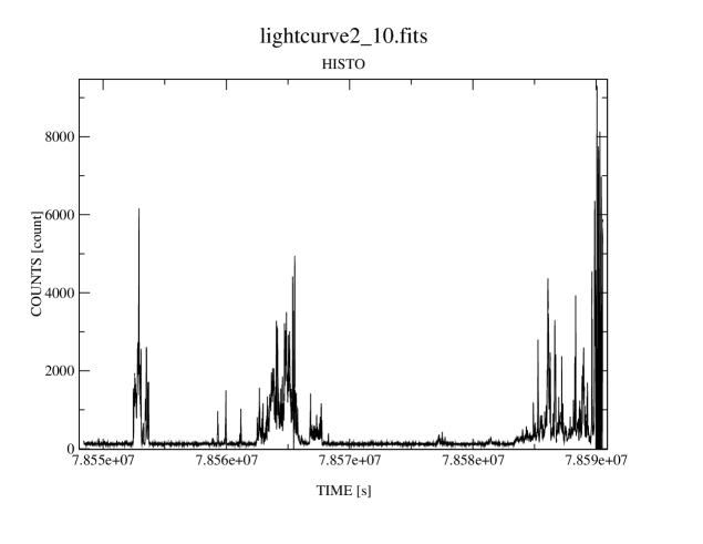
Figure 5.1: Lightcurve binned in 10 s intervals.

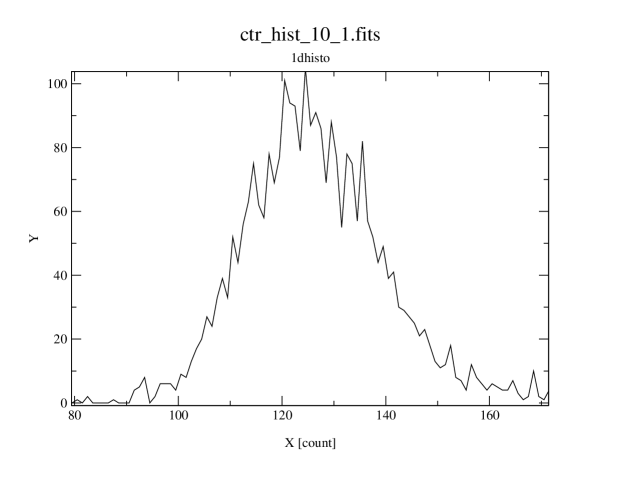
Figure 5.2: Central part of the count rate [counts per 10 s] distribution.

Table 5.1: Observation parameters

ID	Date	R.A.	Dec.	Duration	Exposure	GTI	Detector	Filter
0098010101	2000-06-28	210.2629	2.8507	56 ks	42 ks	25 ks	EPIC-pn FF	Thin

For the spectral analysis all obvious point sources have been excluded as well as hot pixels and columns. Furthermore a correction has been applied to account for events counted during read out (out of time events, most obviously visible as the ‘jet’ extending from the cluster center parallel to the hot column, Fig. 5.3). The correction is done by creating an events file within the XMM SAS (Science Analysis System), where events have been redistributed randomly along columns keeping all other info, e.g., pattern and time. The CTI (Charge Transfer Inefficiency) correction is done after the redistribution. Then a spectrum (or image) created from this events file is multiplied by a mode dependent factor ($=0.06$ for Full Frame mode, FF) and subtracted from the original spectrum (or image). Neglecting the influence of out of time events may lead to wrong temperature estimates since these events are assigned an incorrect CTI correction. Moreover, assume the cluster center has a lower temperature than the outer parts (as will actually be found later), then a spectrum taken from a ring of the outer low surface brightness region is contaminated by photons having a lower energy on average and the temperature estimate may be biased low.

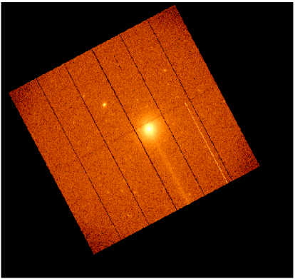
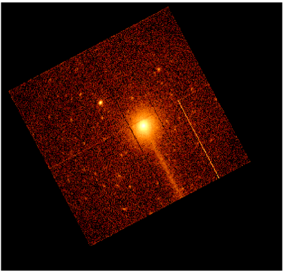
Figure 5.3: EPIC-pn images of A1835 in sky coordinates in the energy band 0.35–10 keV. The field of view is almost 30 arcmin. Left: Full 42 ks observation. Right: 25 ks Good Time Intervals after application of the count rate thresholds.

The subtraction of the (remaining) background is performed using spectra created in the same way as outlined above. Various methods may be applied for background subtraction. The major drawbacks of two simple methods for the observation here are described as follows. One possibility is to use a ‘blank sky’ observation like the Lockman Hole observation and create a spectrum from the same detector region as the source spectrum, scaling by the source spectrum’s exposure time. The disadvantage of this method is that it ignores variation in the Cosmic X-ray Background (CXB). The CXB is mainly composed of A) isotropic extragalactic emission (dominant for photon energies $E\gtrsim 2$ keV) and B) anisotropic emission from galactic diffuse sources and the ‘hot bubble’ around the solar system (important for $E\lesssim 2$ keV). Galactic photoelectric absorption (important for $E\lesssim 1$ keV) causes an additional anisotropy. The CXB therefore can be considered as constant in time but varying with pointing direction (at soft energies) (e.g., Ishisaki, 1997). A further drawback is that a possible temporal variation of the normalization and/or spectrum of the PIB is ignored. Last not least if this method is used one must ensure that the flare filtering criteria are equivalent for science and background observation. This can be achieved, e.g., by assuming a constant PIB and selecting an energy band containing exclusively PIB and soft proton events (possibly $E>12$ keV) with the drawback of a significant loss in statistics. Another simple method for the background subtraction is to use a ring outside the cluster emission in the science observation, taking advantage of the medium redshift of A1835 and XMM-Newton’s field of view. Here the drawbacks are that the structure on the detector of the PIB is ignored. Using this method also the question arises whether or not one should apply a vignetting correction for the background spectrum. If a correction is applied then the actually not vignetted PIB is overestimated. If no correction is applied then the vignetted CXB is underestimated.

More complicated methods are possible circumventing some of the above problems (e.g., Majerowicz and Neumann, 2001; Pratt et al., 2001). Here the background from not vignetting corrected data in a ring where the contribution from cluster emission is negligible (7–11 arcmin from cluster center) has been taken because the PIB dominates the background. The main structural feature of the PIB is a fluorescent copper line at 8 keV, which is almost absent at the detector center but increases towards the outer parts of the EPIC-pn detector. Therefore events with $7.9\leq E\leq 8.1$ keV have been excluded from the fit. With this method the CXB and PIB are corrected for in one step, since the CXB is not expected to change drastically for this small angular distance and variations in the PIB spectrum with time have no effect since exactly equivalent time intervals are used. Note, however, that the absolute contribution of the CXB is underestimated due to the vignetting increase with increasing radius. In the outer parts the fitted value of the column density of neutral hydrogen, $n_{\rm h}$, drops below the galactic value, which indicates that leaving $n_{\rm h}$ as a free parameter compensates for the underestimated CXB. However, the decrease of the $n_{\rm h}$ value is certainly not an ideal correction for this effect, since the spectral changes invoked by both effects probably do not cancel each other exactly. On the other hand using a vignetting corrected background for this method, where photons have been corrected individually, has resulted in worse fits and underestimated temperatures in the outer parts because of the wrongly corrected PIB. This is due to the dominance of the PIB at high energies and to the steeper vignetting increase with radius for higher energies.

Only singles, i.e. photons having deposited their energy in a single pixel on the CCD, have been selected for the spectral analysis. Most events are single events, but the just recently made available response matrix for double events will allow to increase the statistics at least for higher energies and test the effects of a possible dependence of the single to double fraction on detector position soon. A 5-$\sigma$ binning for the spectra has been used to ensure a significant signal in each bin. Choosing a 3-$\sigma$ binning changes the fit results only well within the statistical errors. The energy range used has nominally been set to 0.3–10.0 keV. In the outer low surface brightness parts the number of significant high energy bins decreases. The fit parameter values have therefore been determined partly within smaller energy ranges. If two or more different temperatures are present for a specific radial bin then the availability of only a weak signal at high energies may bias the estimated temperature in the outermost radial bin low. The presence of a lower signal to noise ratio at higher energies is independent of the binning method. The spectra have been modeled and fitted within XSPEC using a single temperature MeKaL model (Mewe et al., 1995) including photoelectric absorption (wabs*mekal). The temperature, metal abundance, absorption column density, and normalization have been left as free parameters. Leaving the redshift as a free parameter yields values consistent with the optically determined redshift and with encouragingly small uncertainties. The 2001-05-07 release of EPIC-pn response matrices has been used. The spectra have not been deprojected, i.e. in the innermost radial bins also contributions from physically larger radii are included. However, the very steep radial surface brightness profile of A1835 ensures that these contaminating contributions are small. Changing the background normalization by $\pm 10$ % has a negligible effect on the fit parameter values. Inclusion of arf files that correct the source spectra for telescope vignetting also affects the parameter values only insignificantly.

5.3 Results and Discussion

Figure 5.4: Temperature profiles as obtained with different detectors. Filled circles: EPIC-pn, this work; open triangles: EPIC-MOS2 (Majerowicz and Neumann, 2001); open diamonds: Chandra (Schmidt et al., 2001). Vertical error bars indicate the 90 % confidence level statistical uncertainty for one interesting parameter for the first two works and the 1-$\sigma$ statistical uncertainty for the last work. Horizontal bars indicate the radial bin size.

The best fit cluster temperatures for six radial bins are shown in Fig. 5.4 as filled circles. The intracluster gas in the center ($r<200$ kpc) is significantly cooler than in the outer parts, which may be caused either by a cooling flow (e.g., Fabian, 1994) or by the Interstellar Medium (ISM) of the central brightest cluster galaxy (e.g., Makishima et al., 2001). Within the statistical uncertainty the temperature profile for $r>200$ kpc can be considered isothermal, in agreement with the assumption made for the mass determination throughout this work. Although at present a temperature decrease in the very outer part obviously cannot be excluded. The main limiting factor for a precise determination of the outer temperature is the relatively high PIB.

Also shown in Fig. 5.4 is the temperature profile determined using data from the EPIC-MOS2 camera onboard XMM-Newton by Majerowicz and Neumann, (2001) (open triangles). There is perfect agreement between the results from the two EPIC cameras out to $\sim 600$ kpc. For larger radii the temperature estimates are well consistent.

The open diamonds in Fig. 5.4 additionally indicate the temperature estimates obtained for A1835 with the Chandra satellite by Schmidt et al., (2001). The agreement in the very center ($r<100$ kpc) between the Chandra and EPIC-pn results is very good. For larger radii Chandra gives systematically higher temperatures, but note that 1-$\sigma$ errors are shown for Chandra.

Using a two temperature model does not result in a significant improvement in any of the EPIC-pn fits, indicating the absence of evidence for gas with $k_{\rm B}T_{\rm X}$ below $\sim 2$ keV. This is in agreement with the results obtained with the RGS (Peterson et al., 2001).

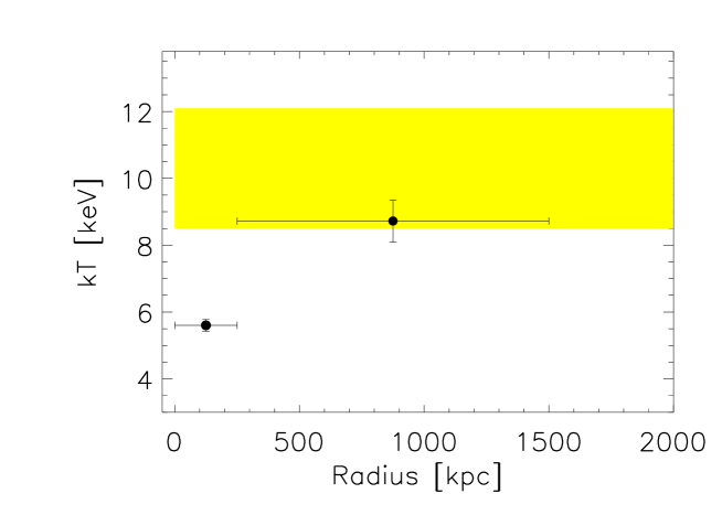
Figure 5.5: Overall gas temperature as estimated with EPIC-pn (upper filled circle; this work) and ASCA (shaded area; Allen et al., 1996).

To obtain a good estimate of the overall cluster temperature outside the central region, where the temperature is assumed to be constant – consistent with observations (Fig. 5.4), a spectrum has been extracted within $250\leq r\leq 1\,500$ kpc. The best fit temperature for this region $k_{\rm B}T_{\rm X}=8.7\pm 0.6$ keV (90 % c.l.). In Fig. 5.5 this result is compared to the previous estimate from ASCA (shaded area; Allen et al., 1996). The ASCA data suggest a higher temperature ($9.8^{+2.3}_{-1.3}$ keV) but the results are consistent. Note that the errors have been decreased significantly with EPIC-pn.

Figure 5.6: Luminosity and temperature of A1835 (open square) as compared to the $L_{\rm X}$–$T_{\rm X}$ relation of 88 clusters compiled during construction of HIFLUGCS.

Figure 5.7: Metal abundance profile as determined with the EPIC-pn camera.

Comparing this overall cluster temperature and A1835’s X-ray luminosity as measured with a ROSAT PSPC pointed observation ($r_{\rm X}=2.85$ Mpc) with the $L_{\rm X}$–$T_{\rm X}$ relation of the part of the clusters in extended sample (Sect. 3) that have measured temperatures one finds that within the scatter it falls nicely onto this relation (Fig. 5.6). Moreover the exceptionally strong central cool emission in A1835 may boost the total X-ray luminosity, which would explain the slightly higher luminosity than expected from the relation.

The metal abundance profile relative to solar abundances (Anders and Grevesse, 1989) is found to be flat within the statistical errors (Fig. 5.7). The mean abundance is about 0.35 solar, in agreement with the value adopted in the flux determination (Sect. 4.1).

5.4 Conclusions

The intracluster gas in the central region is significantly cooler than in the outer part of A1835. The innermost circle with radius 74 kpc yields a temperature estimate $T_{\rm X}=4.3\pm 0.2$ keV. The gas in the outer part is consistent with being isothermal, in agreement with the assumption made for the mass determination throughout this work. No indications for gas temperatures below $\sim 2$ keV have been found. The metal abundance profile is consistent with being flat with $A\approx 0.35$. The cluster temperature within $250\leq r\leq 1\,500$ kpc has been determined as $k_{\rm B}T_{\rm X}=8.7\pm 0.6$ keV. This temperature is almost exactly equal to the temperature of the innermost circle multiplied by a factor of two. However, it is possible that the temperature decreases further a bit for even smaller radii. The significantly reduced error of the overall cluster temperature will allow to put tighter constraints on $H_{0}$ in combination with the SZ effect. Assuming the cluster temperature to stay isothermal beyond 1 500 kpc an estimate of the total gravitational mass has been obtained utilizing the gas density profile determined from a ROSAT PSPC pointed observation. Under the assumption of hydrostatic equilibrium it is found using (2.16) that $M_{\rm tot}=1.3\pm 0.2\times 10^{15}\,h_{50}^{-1}\,M_{\odot}$ within $r_{500}=2.10$ Mpc.

Chapter 6 Results

In this Chapter it is shown that a tight correlation exists between the gravitational cluster mass and the X-ray luminosity. This ensures that HIFLUGCS is essentially selected by cluster mass. Also relations between other physical properties of the clusters are shown. In the last part of this Chapter the cluster mass function is constructed, including the proper treatment of the scatter in the $L_{\rm X}$–$M_{\rm tot}$ relation.

6.1 Mass–Luminosity Relation

Since one of the main aims of this work is the construction of a mass function from a flux-limited sample it is important to test for a correlation between X-ray luminosity and gravitational mass. In Fig. 6.1 $L_{\rm X}$, given in the ROSAT energy band, is plotted as a function of $M_{200}$, showing clearly the existence of a tight (linear Pearson correlation coefficient $=$ 0.92) correlation, as expected.

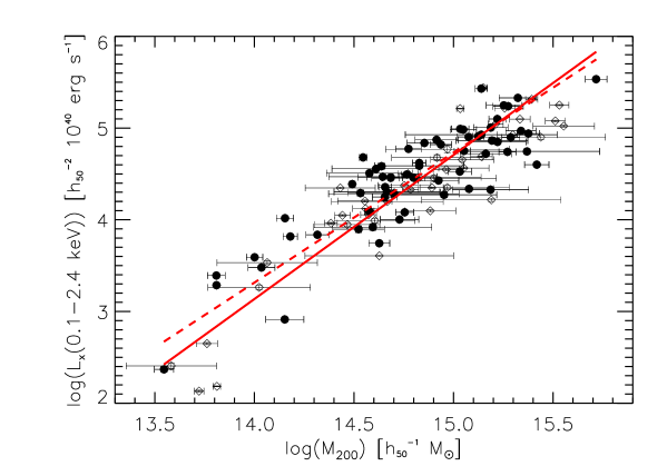
Figure 6.1: Gravitational mass–X-ray luminosity relation (solid line) for the extended sample of 106 galaxy clusters. The dashed line gives the best fit relation for the 63 clusters included in HIFLUGCS (filled circles only). The bisector fit results are shown. One-$\sigma$ statistical error bars are plotted for both axes, however, only the mass errors are larger than the symbol sizes.

To quantify the mass–luminosity relation, a linear regression fit in log–log space has been performed. The method used allows for intrinsic scatter and errors in both variables (Akritas and Bershady, 1996). Tables 6.1–6.5 give the results for different fit methods, where minimization has been performed in vertical, horizontal, and orthogonal direction, and the bisector result is given, which bisects the best fit results of vertical and horizontal minimization. The fits have been performed using the form

$$\log\left(\frac{L_{\rm X}(0.1-2.4\,{\rm keV})}{h_{50}^{-2}\,10^{40}\,{\rm ergs\,s^{-1}}}\right)=A+\alpha\log\left(\frac{M_{200}}{h_{50}^{-1}\,M_{\odot}}\right)\,.$$ (6.1)

It is found, as noted in general by previous authors (e.g., Isobe et al., 1990), that the chosen fitting method has a significant influence on the best fit parameter values. For different applications different fitting methods may be required. In this work the appropriate relation for the application under consideration is always indicated.

The difference between the fit results for 106 (Tab. 6.1) and 63 (Tab. 6.2) clusters may indicate a scale dependence of the $L_{\rm X}$–$M_{\rm tot}$ relation, since the difference is slightly larger than the uncertainty evaluated with the bootstrap method. The small number of low luminosity clusters in HIFLUGCS compared to the extended sample may be responsible for the less steep relation obtained using the HIFLUGCS clusters only. Note that only two out of the six clusters with $L_{\rm X}<h_{50}^{-2}\,10^{43}\,{\rm ergs\,s^{-1}}$ are included in HIFLUGCS. To reliably detect any deviations from the power law shape of the $L_{\rm X}$–$M_{\rm tot}$ relation, however, even more clusters with $M_{\rm tot}<10^{14}\,h_{50}^{-1}\,M_{\odot}$ (and possibly $M_{\rm tot}>3\times 10^{15}\,h_{50}^{-1}\,M_{\odot}$) would need to be sampled. In Sect. 7.3 this will be further discussed. As will be seen later, in the procedure used here for the comparison of observed and predicted mass functions the precise shape of the $L_{\rm X}$–$M_{\rm tot}$ relation is not important.

Table 6.1: Fit parameter values

Fit	$\alpha$	$\Delta\alpha$	$A$	$\Delta A$
BCES($L\mid M$)	1.496	0.089	-17.741	1.320
bootstrap	1.462	0.089	-17.238	1.327
BCES($M\mid L$)	1.652	0.085	-20.055	1.261
bootstrap	1.672	0.086	-20.357	1.278
BCES-Bisector	1.571	0.083	-18.857	1.237
bootstrap	1.562	0.083	-18.717	1.239
BCES-Orthogonal	1.606	0.086	-19.375	1.283
bootstrap	1.609	0.088	-19.419	1.308

Note. — Best fit parameter values and standard deviations for the extended sample (106 clusters) for a fit of the form (6.1). The rows denoted ‘bootstrap’ give the results obtained for 10 000 bootstrap resamplings.

Table 6.2: Fit parameter values

Fit	$\alpha$	$\Delta\alpha$	$A$	$\Delta A$
BCES($L\mid M$)	1.310	0.103	-14.935	1.526
bootstrap	1.256	0.103	-14.146	1.531
BCES($M\mid L$)	1.538	0.105	-18.320	1.568
bootstrap	1.584	0.113	-18.995	1.681
BCES-Bisector	1.418	0.097	-16.536	1.434
bootstrap	1.407	0.096	-16.368	1.427
BCES-Orthogonal	1.460	0.105	-17.157	1.559
bootstrap	1.468	0.110	-17.274	1.633

Note. — Same as Tab. 6.1 but for the purely flux-limited sample (63 clusters).

Table 6.3: Fit parameter values

Fit	$\alpha$	$\Delta\alpha$	$A$	$\Delta A$
BCES($L\mid M$)	1.756	0.091	-21.304	1.350
bootstrap	1.719	0.090	-20.746	1.338
BCES($M\mid L$)	1.860	0.084	-22.836	1.246
bootstrap	1.881	0.084	-23.144	1.250
BCES-Bisector	1.807	0.084	-22.053	1.251
bootstrap	1.797	0.084	-21.899	1.241
BCES-Orthogonal	1.835	0.085	-22.473	1.260
bootstrap	1.841	0.085	-22.563	1.270

Note. — Same as Tab. 6.1 but for $L_{\rm Bol}$.

Table 6.4: Fit parameter values

Fit	$\alpha$	$\Delta\alpha$	$A$	$\Delta A$
BCES($L\mid M$)	1.504	0.089	-17.545	1.298
bootstrap	1.469	0.089	-17.042	1.300
BCES($M\mid L$)	1.652	0.086	-19.708	1.254
bootstrap	1.671	0.086	-19.992	1.260
BCES-Bisector	1.575	0.084	-18.590	1.228
bootstrap	1.565	0.083	-18.445	1.224
BCES-Orthogonal	1.609	0.087	-19.075	1.274
bootstrap	1.611	0.088	-19.109	1.290

Note. — Same as Tab. 6.1 but for $M_{500}$.

Table 6.5: Fit parameter values

Fit	$\alpha$	$\Delta\alpha$	$A$	$\Delta A$
BCES($L\mid M$)	2.001	0.124	-25.484	1.858
bootstrap	1.933	0.126	-24.474	1.897
BCES($M\mid L$)	2.488	0.127	-32.761	1.902
bootstrap	2.519	0.130	-33.223	1.940
BCES-Bisector	2.223	0.118	-28.793	1.773
bootstrap	2.193	0.119	-28.357	1.785
BCES-Orthogonal	2.404	0.129	-31.509	1.938
bootstrap	2.415	0.133	-31.667	1.984

Note. — Same as Tab. 6.1 but for $M_{\rm A}$ for comparison (mass errors have not been taken into account here).

Table 6.6: Measured scatter

Scatter	($L\mid M$)	($M\mid L$)	Bisector
106 clusters included in the extended sample.
$\sigma_{\log M_{\rm tot}}$	0.21	0.21	0.21
$\sigma_{\log L_{\rm X}}$	0.31	0.34	0.32
$\sigma_{\log L/M}$	0.17	0.18	0.17
63 clusters included in HIFLUGCS.
$\sigma_{\log M_{\rm tot}}$	0.22	0.21	0.21
$\sigma_{\log L_{\rm X}}$	0.29	0.32	0.30
$\sigma_{\log L/M}$	0.18	0.18	0.17

Note. — Scatter measured for different relations.

The best fit relation for $L_{\rm Bol}$ (Tab. 6.3) will be discussed in Sect. 7.3. One notes that this relation is steeper than the one for $L_{\rm X}(0.1-2.4\,{\rm keV})$. This is caused by the fact that the bolometric emission coefficient depends stronger on the gas temperature. As expected the relation for $M_{500}$ (Tab. 6.4) has a very similar slope and a higher normalization than the one for $M_{200}$. It is given here for a possible comparison with subsequent works as well as the relation with the formally determined masses within an Abell radius (Tab. 6.5), which is steeper because low luminosity clusters are assigned much higher masses.

When constructing the mass function, the overall (measurement plus intrinsic) scatter in the $L_{\rm X}$–$M_{\rm tot}$ relation may become important (Sect. 6.4). After verifying that the scatter is approximately Gaussian in log space the scatter has been measured as given in Tab. 6.6. The scatter in $L_{\rm X}(0.1-2.4\,{\rm keV})$, $M_{200}$, and orthogonal to the best fit line is given by $\sigma_{\log L_{\rm X}}$, $\sigma_{\log M_{\rm tot}}$, and $\sigma_{\log L/M}$, respectively. The measured scatter does not vary strongly depending on the chosen fitting method. The slight differences are expected qualitatively. For instance $\sigma_{\log L_{\rm X}}$ is smaller for ($L\mid M$) compared to ($M\mid L$) because the best fit is determined by minimizing the residuals in $\log L_{\rm X}$ for the former.

6.2 Intracluster Gas Fraction

An important parameter for the understanding of cluster physics is the amount of intracluster gas relative to the total mass, since for instance heating and cooling processes are likely to affect this gas fraction. The mean gas mass fraction within $r_{200}$ for the extended sample of 106 clusters has been found as $\langle f_{\rm gas}\rangle=0.19\pm 0.08\,h_{50}^{-3/2}$. This parameter is also important for cosmology as outlined in Sect. 7.6.2. In the next two Sections it is tested whether there are systematic variations of the gas fraction.

6.2.1 Variation of Gas Fraction with Mass

In the following relations between various quantities for the 106 galaxy clusters will be shown. Since for 18 clusters the gas temperature has been estimated using a luminosity–temperature relation, these clusters are omitted here and in all other Sections when the temperature is one of the quantities of interest. For a better illustration of possible deviations from pure power laws in some plots non parametric regression fits using a smoothed spline function (e.g., Simonoff, 1996, Sect. 5.6) are shown. These fits have been calculated with the standard statistics software package S-Plus using 5 degrees of freedom and assigning each point the same weight.

Figure 6.2: Gas mass fraction as a function of gravitational mass. The solid line denotes the result of a smoothed spline fit, indicating a break around $2\times 10^{14}\,h_{50}^{-1}\,M_{\odot}$.

Figure 6.3: Gas mass fraction as a function of gas mass. The solid line denotes the result of a smoothed spline fit, indicating a break around $2\times 10^{13}\,h_{50}^{-1}\,M_{\odot}$.

Figure 6.4: Gas mass fraction as a function of gas temperature. The solid line denotes the result of a smoothed spline fit, indicating a break around 2 keV.

In Fig. 6.2 the gas mass fraction is shown as a function of the gravitational mass. Note that the main uncertainty of $M_{{\rm gas},200}$ comes from the uncertainty of $r_{200}$. Therefore the errors of $M_{{\rm gas},200}$ and $M_{200}$ are strongly correlated and combining these errors via standard error propagation is not a useful option for assessing the uncertainty of $f_{\rm gas}$. Since for a given radius the error of the gas mass estimation is much smaller it is neglected here. Rather the error of $f_{\rm gas}$ is determined from the error of $M_{200}$ (including the uncertainty of $r_{200}$).

It is clear from Fig. 6.2 that $f_{\rm gas}\,h_{50}^{1.5}\approx$ 10–30 % for most of the clusters. No clear trend with the gravitational mass is apparent, as long as $M_{\rm tot}\gtrsim 2\times 10^{14}\,h_{50}^{-1}\,M_{\odot}$. For smaller masses, however, a drop of the gas fraction is indicated, even though caused by only 5–6 clusters. A similar behavior is noted if $f_{\rm gas}$ is plotted as a function of the gas mass (Fig. 6.3) and of the gas temperature (Fig. 6.4). Possible reasons for this sudden drop of $f_{\rm gas}$ towards smaller systems are discussed in Sect. 7.4.

6.2.2 Variation of Gas Fraction with Radius

To characterize the extent of the gas relative to the dark matter the ratio $f_{{\rm gas},200}/f_{{\rm gas},500}$ is introduced. This ratio compares the gas fraction at two characteristic radii, i.e. at two radii of constant overdensity. Obviously, since the overdensity decreases with increasing radius, $f_{{\rm gas},200}/f_{{\rm gas},500}>1$ indicates that the gas is more extended than the dark matter.

Figure 6.5: Gas fraction within $r_{200}$ divided by the gas fraction within $r_{500}$ as a function of $M_{200}$. For most of the clusters the gas fraction increases with radius but for some of the high mass clusters there are indications for a decrease. The result of a smoothed spline fit is shown as solid line.

In Fig. 6.5 this ratio is plotted as a function of gravitational mass. Note that the errors of $f_{{\rm gas},200}$ and $f_{{\rm gas},500}$ are strongly correlated. Only the error in $f_{{\rm gas},500}$ is therefore taken into account for the calculation of the uncertainty of $f_{{\rm gas},200}/f_{{\rm gas},500}$. The statistical errors still seem larger than the actual scatter of the points. This may be caused by the fact that the uncertainty in $r_{500}$ is not neglected.

One notes that for most of the clusters the gas fraction is larger at larger radii. For some clusters, however, the dark matter seems to be more extended than the gas. Note that taking into account the error bars no cluster has $f_{{\rm gas},200}/f_{{\rm gas},500}$ significantly lower than 1. Interestingly, however, there appears to be a systematic trend for the larger systems that the gas extent becomes smaller with increasing mass relative to the dark matter extent. This apparent trend will be discussed further in Sect. 7.4.

6.3 Relations between Shape Parameters, Temperature, Luminosity, and Mass

In this Section various relations between the parameters describing the surface brightness (and therefore gas density) profile, $\beta$ and $r_{\rm c}$, the gas temperature, X-ray luminosity, gas and gravitating mass will be presented. The implications of the trends seen here will be discussed in Sect. 7.5.

Figure 6.6: $\beta$ versus core radius. Solid line: Best fit parabolic model ($\beta_{0}=0.55$, $r_{\rm s}=885$ kpc) of Neumann and Arnaud, (1999), dashed line: same model with $\beta_{0}=0.57$, $r_{\rm s}=775$ kpc. Dot-dashed line: smoothed spline fit.

A correlation between the two fit parameters $\beta$ and $r_{\rm c}$ as induced by the fitting process is indicated by the confidence contours (Fig. 4.5). However, the typical uncertainty is much smaller than the range of $\beta$ and $r_{\rm c}$ values spanned by the sample. The origin of the correlation present in Fig. 6.6 may therefore be physical. Using a sample of 26 galaxy clusters Neumann and Arnaud, (1999) showed that a physical correlation exists and determined best fit parameters of the function

$$\beta=\beta_{0}\left[1+(r_{\rm c}/r_{\rm s})^{2}\right]$$ (6.2)

as given in the caption of Fig. 6.6. The smoothed spline fit shown in Fig. 6.6 indicates that this parameterization accounts well for the trend seen. However, for the 106 clusters used here a different set of parameter values appears to provide a better description of the data.

Figure 6.7: Core radius versus temperature. The two parameters are clearly correlated.

Figure 6.8: Core radius versus gravitational mass. The positive correlation is obvious.

Figs. 6.7 and 6.8 clearly show that the core radius is correlated with cluster temperature and mass. The temperature and core radius are determined completely independent from one another. Also the gravitational mass estimate is effectively independent of $r_{\rm c}$ at large radii ($r\gg r_{\rm c}$; Eq. 2.16). A significant portion of the scatter present in these Figures is probably due to the presence (smaller $r_{\rm c}$) or absence (larger $r_{\rm c}$) of a central excess emission. First results of a cooling flow study of the HIFLUGCS clusters indicate a respective trend (Y. Chen et al., in preparation).

Figure 6.9: The fit parameter $\beta$ is plotted versus the gravitational mass. A smoothed spline fit is shown as solid line, indicating a possible trend at the high mass side.

Figure 6.10: $\beta$ versus the intracluster gas temperature. A smoothed spline fit is shown as solid line. No clear trends are indicated, except a very weak indication for the hottest clusters.

In Fig. 6.9 $\beta$ is plotted as a function of $M_{200}$. Also shown is the result of a smoothed spline fit. For $M_{200}\lesssim 3\times 10^{14}\,h_{50}^{-1}\,M_{\odot}$ there is no indication of any trend of $\beta$ with mass. For larger masses $\beta$ appears to increase with increasing mass. Note that $\beta$ is used for the calculation of the gravitational mass (Eq. 2.16). The X-ray temperature determination does not depend on $\beta$ (except possibly through the modeling of the surface brightness profile often performed to calculate the effective area for ASCA observations). Shown in Fig. 6.10 is $\beta$ versus $T_{\rm X}$, indicating that the two parameters are almost independent of one another. For the hottest clusters there is, however, a weak suggestion of a trend in the same sense as in the previous plot.

The plot $L_{\rm X}(0.1-2.4\,{\rm keV})$ versus $T_{\rm X}$ has already been shown in Sect. 5.3. The corresponding best fit relations, determined using the linear regression method described in Sect. 6.1, are given in Tab. 6.7. In Fig. 6.11 the bolometric X-ray luminosity is shown as a function of the gas temperature. The relation seems to be well represented by a power law of the form $L_{\rm Bol}\propto T_{\rm X}^{3}$ (Tab. 6.8) over the entire temperature range.

Figure 6.11: Bolometric X-ray luminosity versus temperature. The solid line represents the best fit result using the bisector method.

Fig. 6.12 shows that the X-ray luminosity and the gas mass are tightly correlated. The best fit relations are given in Tab. 6.9. Knowing already that there exist correlations between luminosity and temperature and between luminosity and gas mass it is not a big surprise that the gas mass correlates well with the temperature. This relation is graphically shown in Fig. 6.13 and tabulated in Tab. 6.10. Note that in principal $M_{\rm gas}$ and $T_{\rm X}$ are determined almost independent from one another. However, since $r_{200}$ depends strongly on $T_{\rm X}$ clearly also the calculation of $M_{{\rm gas},200}$ depends on $T_{\rm X}$.

Figure 6.12: X-ray luminosity versus gas mass in the energy band ($0.1-2.4\,{\rm keV}$). The solid line represents the best fit result using the bisector method.

Figure 6.13: Gas temperature versus gas mass. The solid line represents the best fit result using the bisector method.

Another relation of specific interest is the $M_{\rm tot}$–$T_{\rm X}$ relation. Its relevance derives not only from its importance in the study of physical processes but also from its role in the context of the interpretation of temperature functions (analogous to mass functions, see Sect. 6.4). If one wants to use temperature functions to determine cosmological parameters, in some way the connection between temperature and mass has to be made. This may be done using theoretical predictions, simulations, or observations. It is therefore important to test the consistency of the different $M_{\rm tot}$–$T_{\rm X}$ relations. In Fig. 6.14 the data points and the corresponding best fit relation (Tab. 6.11) are shown.

Figure 6.14: Gas temperature versus gravitational mass. The solid line represents the best fit result using the bisector method.

Table 6.7: Fit parameter values

Fit	$\alpha$	$\Delta\alpha$	$A$	$\Delta A$
BCES($L\mid T$)	2.481	0.130	2.862	0.093
bootstrap	2.367	0.132	2.934	0.095
BCES($T\mid L$)	2.724	0.128	2.708	0.091
bootstrap	2.766	0.131	2.682	0.093
BCES-Bisector	2.598	0.125	2.788	0.089
bootstrap	2.552	0.124	2.817	0.089
BCES-Orthogonal	2.692	0.129	2.728	0.092
bootstrap	2.712	0.132	2.716	0.094

Note. — Best fit parameter values and standard deviations for the 88 clusters with measured temperatures for a fit of the form

$\log\left(\frac{L_{\rm X}(0.1-2.4\,{\rm keV})}{h_{50}^{-2}\,10^{40}\,{\rm ergs\,s^{-1}}}\right)=A+\alpha\log\left(\frac{T_{\rm X}}{{\rm keV}}\right)$.

The rows denoted ‘bootstrap’ give the results obtained for 10 000 bootstrap resamplings.

Table 6.8: Fit parameter values

Fit	$\alpha$	$\Delta\alpha$	$A$	$\Delta A$
BCES($L\mid T$)	2.906	0.126	2.898	0.090
bootstrap	2.776	0.126	2.981	0.091
BCES($T\mid L$)	3.067	0.122	2.797	0.088
bootstrap	3.109	0.125	2.770	0.090
BCES-Bisector	2.984	0.121	2.849	0.087
bootstrap	2.933	0.120	2.881	0.087
BCES-Orthogonal	3.050	0.123	2.808	0.088
bootstrap	3.074	0.125	2.792	0.090

Note. — Best fit parameter values and standard deviations for the 88 clusters with measured temperatures for a fit of the form

$\log\left(\frac{L_{\rm Bol}(0.01-40\,{\rm keV})}{h_{50}^{-2}\,10^{40}\,{\rm ergs\,s^{-1}}}\right)=A+\alpha\log\left(\frac{T_{\rm X}}{{\rm keV}}\right)$.

Table 6.9: Fit parameter values

Fit	$\alpha$	$\Delta\alpha$	$A$	$\Delta A$
BCES($L\mid M$)	1.118	0.034	-11.291	0.482
bootstrap	1.104	0.033	-11.096	0.460
BCES($M\mid L$)	1.162	0.038	-11.907	0.533
bootstrap	1.184	0.043	-12.221	0.606
BCES-Bisector	1.140	0.035	-11.596	0.500
bootstrap	1.143	0.036	-11.647	0.515
BCES-Orthogonal	1.143	0.036	-11.637	0.513
bootstrap	1.149	0.039	-11.727	0.546

Note. — Best fit parameter values and standard deviations for the 106 clusters of the extended sample for a fit of the form

$\log\left(\frac{L_{\rm X}(0.1-2.4\,{\rm keV})}{h_{50}^{-2}\,10^{40}\,{\rm ergs\,s^{-1}}}\right)=A+\alpha\log\left(\frac{M_{{\rm gas},200}}{h_{50}^{-5/2}\,M_{\odot}}\right)$.

Table 6.10: Fit parameter values

Fit	$\alpha$	$\Delta\alpha$	$A$	$\Delta A$
BCES($M\mid T$)	2.230	0.106	12.654	0.075
bootstrap	2.126	0.113	12.721	0.081
BCES($T\mid M$)	2.246	0.115	12.644	0.081
bootstrap	2.276	0.115	12.626	0.081
BCES-Bisector	2.238	0.108	12.649	0.077
bootstrap	2.199	0.112	12.675	0.080
BCES-Orthogonal	2.243	0.112	12.645	0.080
bootstrap	2.250	0.116	12.643	0.082

Note. — Best fit parameter values and standard deviations for the 88 clusters with measured temperatures for a fit of the form

$\log\left(\frac{M_{{\rm gas},200}}{h_{50}^{-5/2}\,M_{\odot}}\right)=A+\alpha\log\left(\frac{T_{\rm X}}{\rm keV}\right)$.

Table 6.11: Fit parameter values

Fit	$\alpha$	$\Delta\alpha$	$A$	$\Delta A$
BCES($M\mid T$)	1.710	0.058	13.735	0.041
bootstrap	1.641	0.052	13.778	0.037
BCES($T\mid M$)	1.591	0.052	13.811	0.036
bootstrap	1.633	0.055	13.784	0.038
BCES-Bisector	1.649	0.046	13.774	0.033
bootstrap	1.637	0.046	13.781	0.033
BCES-Orthogonal	1.622	0.046	13.791	0.032
bootstrap	1.635	0.048	13.782	0.034

Note. — Best fit parameter values and standard deviations for the 88 clusters with measured temperatures for a fit of the form

$\log\left(\frac{M_{200}}{h_{50}^{-1}\,M_{\odot}}\right)=A+\alpha\log\left(\frac{T_{\rm X}}{{\rm keV}}\right)$.

6.4 Mass Function

In Sect. 6.1 it has been shown that the X-ray luminosity is closely correlated with cluster mass. Therefore the $V_{\rm max}$ estimator (Sect. 2.2.3.1) can also be applied to estimate the mass function; $V_{\rm max}$ then being a function of mass. Three different methods have been employed here to correct for the scatter present in the $L_{\rm X}$–$M_{\rm tot}$ relation. If $V_{\rm max}(L_{\rm X})$ is used instead of $V_{\rm max}(M_{\rm tot})\equiv V_{\rm max}(L(M_{\rm tot}))$, where $L(M_{\rm tot})$ is the luminosity estimated from the $L_{\rm X}$–$M_{\rm tot}$ relation using the determined cluster mass $M_{\rm tot}$, the scatter is automatically taken into account. This method has been widely used in the construction of X-ray temperature functions, recently, e.g., by Henry, (2000). If $V_{\rm max}(M_{\rm tot})$ is used and the utilized $L_{\rm X}$–$M_{\rm tot}$ relation is assumed to be the ‘true’ relation then the scatter in this relation has to be taken into account explicitly. Therefore following the method employed for the temperature function by Markevitch, (1998) and Ikebe et al., (2001) the mass function may also be estimated by determining $V_{\rm max}^{\ast}(M_{\rm tot})$, where the measured scatter in $\log L_{\rm X}$ is included. Specifically

$$V_{\rm max}^{\ast}(M_{\rm tot})\equiv\int^{\infty}_{-\infty}V_{\rm max}(L^{\prime})\,(2\pi\sigma_{\log L_{\rm X}}^{2})^{-1/2}$$

$$\times\ \exp\left({-\frac{(\log L^{\prime}-(A+40)-\alpha\log M_{\rm tot})^{2}}{2\sigma_{\log L_{\rm X}}^{2}}}\right)\,d\log L^{\prime}$$ (6.3)

has been used, where $A$ and $\alpha$ are the best fit parameter values taken from the appropriate $L_{\rm X}$–$M_{\rm tot}$ relation of the form (6.1) and $\sigma_{\log L_{\rm X}}$ is the corresponding measured standard deviation in $\log L_{\rm X}$ given in Tab. 6.6.

Now say that for a cluster at redshift $z_{1}$ to be included in the flux-limited sample it must have $L_{\rm X}\geq L_{1}$. Then consider the redshift shells $z_{1}-dz$ (shell A) and $z_{1}+dz$ (shell B). The volume enclosed by shell B is larger than the volume enclosed by shell A. This means that shell B contains more clusters with mass $M_{1}$ which corresponds to $L_{1}$. However due to measurement and intrinsic scatter clusters with $M_{1}$ may be assigned a range of different luminosities $L_{0}\leq L_{1}\leq L_{2}$. As long as $L_{1}-L_{0}\leq L_{2}-L_{1}$, which is satisfied here since the scatter in $L$ is roughly Gaussian in log space, this implies that more clusters with $M_{1}$ from shell B will be included in the sample than clusters with $M_{1}$ from shell A. This further implies that the counted clusters with $M_{1}$ have a mean $L$ slightly larger than $L_{1}$. Therefore the measured normalization of an $L$–$M$ relation constructed with these clusters is expected to be slightly higher than the measured normalization of an $L$–$M$ relation constructed with a volume-limited sample. This also implies that if the former $L$–$M$ relation is used to calculate $V_{\rm max}$ one gets on average a larger $V_{\rm max}$. This means the effect of the scatter in the $L$–$M$ relation is already taken into account if the $L$–$M$ relation determined using the flux-limited sample is used for the calculation of $V_{\rm max}(M_{\rm tot})$.

The drawback of using $V_{\rm max}(L_{\rm X})$ is that a small number of clusters per mass bin possibly does not represent the true scatter well. To minimize this effect here at least ten clusters per mass bin are used. The drawback of using $V_{\rm max}^{\ast}(M_{\rm tot})$ or $V_{\rm max}(M_{\rm tot})$, as noted by Markevitch, (1998), is the reliance on the validity of the measured relation over the entire mass range. The first method and the method that accounts for the scatter explicitly (Eq. 6.3) have been tested by using Monte Carlo simulations for a precisely known $L_{\rm X}$–$T_{\rm X}$ relation and scatter and have been shown to give accurate estimates of $\phi(T)$ for a large number of clusters in the study of the HIFLUGCS temperature function by Ikebe et al., (2001).

In Fig. 6.15 the HIFLUGCS mass functions determined by the two approaches using $V_{\rm max}(L_{\rm X})$ and $V_{\rm max}(M_{\rm tot})$ are shown. Each bin contains 10 clusters, apart from the highest mass bin, which contains 11 clusters. The highest and lowest mass clusters of the 63 clusters contained in the sample have been used to calculate the highest and lowest mass intervals. E.g., the high mass boundary of the highest mass interval is determined by adding half the difference between the largest and second largest mass to the second largest mass.

As expected the method employing $V_{\rm max}(L_{\rm X})$ prompts a mass function exhibiting a larger scatter, because in this case the scatter is accounted for by the actual scatter of the ten or eleven clusters in each mass bin. For comparison the two extreme mass functions calculated using $V_{\rm max}(M_{\rm tot})$ are shown. Extreme is meant in the sense of using the steepest (A) and shallowest (B) $L_{\rm X}$–$M_{\rm tot}$ relation for the HIFLUGCS sample, i.e. ($M\mid L$) with $\alpha=1.538$ and ($L\mid M$) with $\alpha=1.310$ (Tab. 6.2). At the low mass end (A) predicts a lower luminosity for a given mass than (B) resulting in a smaller $V_{\rm max}$ and therefore a higher $dn/dM$. At the high mass side the effect is opposite resulting in a lower $dn/dM$ for (A). The differences of these mass functions to the mass function calculated using $V_{\rm max}(L_{\rm X})$ can be understood in a similar way and are caused partly by the indication of a deviation from a power law shape of the $L_{\rm X}$–$M_{\rm tot}$ relation. Using $V_{\rm max}^{\ast}(M_{\rm tot})$ results in similar mass functions as shown for the open symbols in Fig. 6.15 but the points lie systematically lower because the scatter is accounted for twice; first by using an $L_{\rm X}$–$M_{\rm tot}$ relation derived from a flux-limited sample and secondly explicitly by weighting with a Gaussian function. For the comparison of the observational mass function to mass functions predicted by certain cosmological models $V_{\rm max}(L_{\rm X})$ is used because it is independent of the precise shape of the $L_{\rm X}$–$M_{\rm tot}$ relation and also because $L_{\rm X}$ has a much smaller measurement uncertainty than $M_{\rm tot}$. The influence of the choice of the $V_{\rm max}$ calculation on the estimation of cosmological parameters is investigated in Sect. 7.6.2.

Figure 6.15: Gravitational mass functions for HIFLUGCS. The mass function plotted with filled circles has been determined using $V_{\rm max}(L_{\rm X})$, the ones with open symbols using $V_{\rm max}(M_{\rm tot})$, where triangles correspond to the relation ($L\mid M$) and squares to ($M\mid L$) both for the flux-limited sample (see text Sect. 6.4). Vertical error bars correspond to the formal 1-$\sigma$ Poisson errors, the horizontal bars indicate the mass intervals covered.

Fig. 6.15 shows that the mass function is decreasing fast with increasing mass, indicating that massive clusters are very rare objects. This fact shows an advantage of using a flux-limited sample for the construction of the mass function. The survey volume is largest for the most luminous – and therefore most massive – clusters. Thus the survey volume is largest for the rarest objects. Construction of a volume-limited cluster sample that samples the whole mass range at least equally well would require adding $\gtrsim 10\,000$ clusters (for instance sampling 10 clusters with $M_{200}\approx 2\times 10^{15}\,h_{50}^{-1}\,M_{\odot}$ implies sampling $\sim 10\,000$ clusters with $M_{200}\approx 2\times 10^{13}\,h_{50}^{-1}\,M_{\odot}$ in a volume-limited sample).

Chapter 7 Discussion

A precise determination of distribution functions requires a high sample completeness. In Sect. 7.1 several completeness tests for HIFLUGCS are discussed, indicating a high completeness. In Sect. 7.2 the cluster masses determined here are compared to independent determinations. The observed $L_{\rm X}$–$M_{\rm tot}$ relation is compared to expectations in Sect. 7.3 and possible applications are indicated. Implications from the measured mean cluster mass to light ratio are outlined. Physical properties of the cluster sample are discussed in Sects. 7.4 and 7.5. The cluster mass function is compared to previous determinations and to predictions of cosmological models in Sect. 7.6. Cosmological inferences from the mean cluster gas mass fraction are given. The total gravitational mass contained in galaxy clusters is compared to the total mass in the universe in Sect. 7.7.

7.1 Sample Completeness

The sample completeness is important for the accuracy of the mass function. The selection criteria detailed in Sect. 3 are met by 63 clusters with mean redshift $\langle z\rangle=0.05$ and with two clusters having $z>0.1$. The sample is constructed from surveys with much deeper flux limits and high completenesses. A possible remaining incompleteness in these surveys is likely to be present at low fluxes close to their flux limits, which therefore would not effect HIFLUGCS. Nevertheless four completeness tests have been performed and are described in this Section; they all indicate a high completeness of HIFLUGCS. The $\log N-\log S$ and $L_{\rm X}-z$ diagram are compared to expectations, the luminosity function is compared to luminosity functions of deeper surveys, and the $V/V_{\rm max}$ test is performed.

Figure 7.1: $\log N(>f_{\rm X})-\log f_{\rm X}$ diagram. Fluxes are measured in the ROSAT energy band ($0.1-2.4\,{\rm keV}$). The dashed line has a slope $-1.5$, expected for a uniform distribution of clusters in a static Euclidean universe (‘three-halves-law’), the line is normalized to produce the same cluster number at $f_{\rm X}=8\times 10^{-11}\,{\rm ergs\,s^{-1}\,cm^{-2}}$.

Figure 7.1 shows the integral number counts as a function of X-ray flux (‘$\log N-\log S$’). The slope in the $\log N-\log S$ diagram is very close to the value $-1.5$ expected in a static Euclidean universe for uniformly distributed clusters. Due to the small number of clusters (4) the deviation is not significant for $f_{\rm X}\gtrsim 1\times 10^{-10}\,{\rm ergs\,s^{-1}\,cm^{-2}}$. Since the average redshift is smallest for the highest fluxes large scale structure is not completely washed out at the high flux end, therefore the slight bump visible around $f_{\rm X}\sim 6\times 10^{-11}\,{\rm ergs\,s^{-1}\,cm^{-2}}$ in Fig. 7.1 suggests a deviation caused by cosmic variance. The effect of an expanding and finite universe on the $\log N-\log S$ – flattening of the slope towards low fluxes – is small for the redshift range covered by the sample. The slope consistent with $-1.5$ towards the flux limit therefore indicates a high completeness of HIFLUGCS.

In Fig. 7.2 the X-ray luminosity is plotted as a function of redshift. The flux limit is shown as a solid line.

Figure 7.2: X-ray luminosity as a function of redshift. The flux limit is shown as a solid line.

One notes the increase in rare luminous systems with increasing redshift (volume). Because of the seeming underdensity of clusters in the redshift range $0.10<z<0.15$ a comparison with the expected number of clusters as derived from $N$-body simulations has been performed. An OCDM simulation, carried out for analysis of the power spectral densities of REFLEX clusters (Schuecker et al., 2001b ), adjusted to the HIFLUGCS survey volume in the southern hemisphere (roughly half of the total volume sampled by HIFLUGCS) has been used. The simulation yields 39 clusters while 33 HIFLUGCS clusters have been detected in this region. It is found that in fact not even one cluster with $z>0.1$ is expected for this volume based on this simulation and the HIFLUGCS subsample also does not contain any cluster with a redshift larger than 0.1. This is a further piece of evidence for the high completeness of the sample.

In Fig. 7.3 the HIFLUGCS X-ray luminosity function is compared to luminosity functions of larger surveys in the southern (REFLEX, Böhringer et al., 2001a ) and northern (BCS, Ebeling et al., 1997) hemisphere. These surveys have much deeper flux limits (Sect. 3) and contain many more clusters. Very good agreement is found, which shows the high completeness and homogeneous selection of HIFLUGCS.

Figure 7.3: X-ray luminosity function for HIFLUGCS compared to surveys with deeper flux limits in the northern (N) and southern (S) hemisphere. Vertical error bars correspond to the formal 1-$\sigma$ Poisson errors (no cosmic variance), the horizontal bars indicate the luminosity intervals covered.

The $V/V_{\rm max}$ test (e.g., Rowan-Robinson, 1968; Schmidt, 1968; Avni and Bahcall, 1980; Peacock, 1999, Sect. 14.5) can be used to asses a possible sample incompleteness. Assuming a uniform distribution of clusters a value 1/2 is expected on average. For HIFLUGCS $\langle V/V_{\rm max}\rangle=0.47\pm 0.04$, which is consistent with the expectation and this result is interpreted as a clear sign that HIFLUGCS covers a large enough volume for most of the $L_{\rm X}$ range to be representative of the local Universe with a high sample completeness. The local nature of HIFLUGCS becomes obvious by noting that the result of the comoving $V/V_{\rm max}$ test is almost identical to the result of the equivalent test assuming a Euclidean and non expanding space, i.e. $\langle(f_{\rm X}/f_{\rm X,lim})^{-3/2}\rangle=0.46$.

7.2 Comparison of Mass Determinations

Next to a high sample completeness, reliable mass estimates are obviously important for the construction of the cluster mass function. In Sect. 2.1.3 it has been outlined that simulations show that X-ray mass estimates as performed in this work generally yield unbiased results with a relatively small scatter. In this Section masses for clusters determined using a similar method by different authors and using a completely independent method are directly compared to the results obtained here. Below a method for a proper comparison is described. In Sects. 7.2.1 and 7.2.2 the results of the comparisons with masses determined using X-ray and optical data, respectively, are given.

Let us assume having two different measurement methods, $A$ and $B$. For a sample of objects simply calculating the mean of the ratios of the results, $M^{A}$ and $M^{B}$, of these two measurement methods, i.e. $\left\langle\frac{M^{A}}{M^{B}}\right\rangle$ (and clearly the ratio of the means, $\frac{\langle M^{A}\rangle}{\langle M^{B}\rangle}$), is not the ideal way for a comparison. Consider for instance the measurement results for two objects $(X_{1},X_{2})$, $M^{A}=(a,1/a)$ and $M^{B}=(1,1)$. Both following means are always equal in this case and depending on $a$ they can be arbitrarily different from 1, i.e.

$$\left\langle\frac{M^{A}}{M^{B}}\right\rangle=\left\langle\frac{M^{B}}{M^{A}}\right\rangle\left\{\begin{array}[]{l@{\quad:\quad}l}=1&a=1\,,\\ >1&a>1\,,\\ <1&a<1\,.\end{array}\right.$$ (7.1)

E.g. for $a=2$ the former mean would imply that method $A$ yields on average results which are a factor of 1.25 larger than method $B$. A calculation of the latter mean would imply exactly the opposite. Using $\log M^{i}$ instead of $M^{i}$ to calculate the above means avoids these apparently qualitatively contradicting results, but the results still differ quantitatively depending on which mean is calculated and they cannot be interpreted in a way that the values for the different measurement methods differ by a constant factor. Therefore here results of different measurements are compared using the mean and standard deviation of the differences of the logarithmic values, i.e.

$${\rm MD}(M^{A},M^{B})\equiv\langle\log M^{A}-\log M^{B}\rangle\,,$$ (7.2)

which is straightforward to interpret (${\rm MD}(M^{A},M^{B})=b\Rightarrow M^{A}=10^{b}M^{B}$ on average) and gives self consistent (${\rm MD}(M^{A},M^{B})=-{\rm MD}(M^{B},M^{A})$) results.

7.2.1 X-Ray Masses

The extended sample has 28 clusters in common with the sample analyzed independently by Finoguenov et al., (2001). Independent is meant in the sense that different people have reduced and analyzed the data while the data themselves were obtained from the same satellite observatories, ROSAT and ASCA. Figure 7.4 shows a comparison of isothermal mass estimates within $r_{200}$ for these clusters. The differences of the logarithmic values are plotted as a function of the mean logarithmic mass in Fig. 7.5. There is no indication of a correlation between these two quantities. Calculation of the mean difference according to (7.2) yields ${\rm MD}(M^{\rm F},M^{\rm R})=0.027\pm 0.113$, indicating that $M^{\rm F}=1.06^{+0.32}_{-0.24}\,M^{\rm R}$ on average for masses determined within $r_{200}$. The standard deviation is almost exactly equal to the size of the mean statistical mass measurement errors found in Sect. 4.2. This result shows that even comparing mass determinations for individual clusters not many significant differences are found. On average the results show very good agreement.

Figure 7.4: Mass determination for 28 groups and clusters. $M^{\rm R}$ denotes masses determined in this work and $M^{\rm F}$ masses determined by Finoguenov et al., (2001).

Figure 7.5: Differences of individual mass estimates.

Finoguenov et al., (2001) determined masses not only by employing the assumption of isothermality, $M^{\rm F,iso}$, but also using measured cluster gas temperature profiles, $M^{\rm F,grad}$. A comparison for 38 clusters included in their sample yields ${\rm MD}(M^{\rm F,grad},M^{\rm F,iso})=-0.097\pm 0.099$, indicating $M^{\rm F,grad}=0.799^{+0.21}_{-0.16}\,M^{\rm F,iso}$ on average. The influence of a possible overestimation of masses determined here on the final determination of cosmological parameters is investigated in Sect. 7.6.2.

7.2.2 Optical Masses

Girardi et al., 1998b determined virial masses for a sample of nearby galaxy clusters by compiling optical velocity dispersions of cluster galaxies from the literature. Figure 7.6 shows a comparison of the mass determinations for 42 clusters common to their sample and the extended sample presented here. No trend in the difference of the logarithmic values with mass is seen in Fig. 7.7. A calculation of the mean difference yields ${\rm MD}(M^{\rm G},M^{\rm R})=0.098\pm 0.283$, indicating that $M^{\rm G}=1.25^{+1.15}_{-0.60}\,M^{\rm R}$ on average.

Figure 7.6: Mass determination for 42 clusters. $M^{\rm R}$ denotes masses determined in this work and $M^{\rm G}$ masses determined by Girardi et al., 1998b .

Figure 7.7: Differences of individual mass estimates.

This result shows that comparing mass determinations for individual clusters one may find significant differences. The average offset between the methods is of about the same size as the mean statistical errors found for the extended sample. The optical masses are about 25 % higher on average. Note, however, that since both measurements aim for determination of the virial mass, no rescaling of radii has been performed, i.e. masses are not determined at the same radius for each method, since this would underestimate the offset and standard deviation of the measurements as needed here. Moreover all clusters in common are compared, i.e. critical cases like A548w, which is part of the larger complex structure of A548 (e.g., Davis et al., 1995), and A2319, known to host a subcluster (e.g., Oegerle et al., 1995), have not been excluded. These two cases constitute the two upper extreme clusters in Fig. 7.7. The three lower extreme cases are A754, a famous cluster undergoing a major merger event (e.g., Henry and Briel, 1995), A2589, which shows no obvious indications of irregularity, except a velocity of the central cD galaxy offset of the cluster core velocity by about 50 % of the cluster velocity dispersion (e.g., Capelato et al., 1991), and A3921, which has been found to be in the state of merging (e.g., Arnaud et al., 1996). Note also that the simple calculation of ${\rm MD}$ assigns each cluster the same weight, i.e. the uncertainty of the mass measurements is neglected. It is worth noting that $\left\langle\frac{M^{\rm R}}{M^{\rm G}}\right\rangle=1.001\pm 0.787$, misleadingly implying the complete absence of any systematic differences between the two measurement methods. The influence of a possible underestimation of masses as determined here on the determination of cosmological parameters is investigated in Sect. 7.6.2. Note that the isothermal mass measurements as performed here lie almost exactly in between the results using gas temperature gradients and using velocity dispersions on average.

7.3 Mass–Luminosity Relation

The close correlation between the X-ray luminosity and the gravitational mass found in Sect. 6.1 is not surprising. If clusters form by collapse when exceeding a common overdensity threshold (neglecting any redshift dependence for now), e.g., by spherical collapse (Eqs. 2.55 and 2.56) but also any other kind of collapse from an overdensity independent of mass, then all clusters will share the same mean density. This picture implies that the cluster mass is proportional to its volume. Therefore

$$M_{\rm tot}\propto R_{\rm ch}^{3}\,,$$ (7.3)

where $R_{\rm ch}$ is the virial radius, but for self similar clusters it could be any characteristic radius, e.g., the core radius. With the assumption of virial equilibrium one has

$$T_{\rm gas}\propto M_{\rm tot}R_{\rm ch}^{-1}\,.$$ (7.4)

Combining (7.3) with bremsstrahlung emission,

$$L_{\rm Bol}\propto\rho_{\rm gas}^{2}T^{1/2}R_{\rm ch}^{3}\quad{\rm and}\quad L_{\rm X}(0.1-2.4\,{\rm keV})\propto\rho_{\rm gas}^{2}R_{\rm ch}^{3}$$ (7.5)

(Sect. 2.1.2.1), where $L_{\rm Bol}$ is the bolometric luminosity, one has

$$L_{\rm Bol}\propto\rho_{\rm gas}^{2}T^{1/2}M_{\rm tot}\quad{\rm and}\quad L_{\rm X}(0.1-2.4\,{\rm keV})\propto\rho_{\rm gas}^{2}M_{\rm tot}\,.$$ (7.6)

Using $\rho_{\rm gas}\propto M_{\rm gas}R_{\rm ch}^{-3}$, (7.3), and (7.4) the relations

$$L_{\rm Bol}\propto f_{\rm gas}^{2}M_{\rm tot}^{4/3}\quad{\rm and}\quad L_{\rm X}(0.1-2.4\,{\rm keV})\propto f_{\rm gas}^{2}M_{\rm tot}$$ (7.7)

follow from (7.6). In this simple picture one therefore expects a correlation between luminosity and mass. For later use note that from (7.3) and (7.4) one finds

$$M_{\rm tot}\propto T_{\rm gas}^{3/2}$$ (7.8)

and, combined with (7.7),

$$L_{\rm Bol}\propto f_{\rm gas}^{2}T_{\rm gas}^{2}\quad{\rm and}\quad L_{\rm X}(0.1-2.4\,{\rm keV})\propto f_{\rm gas}^{2}T_{\rm gas}^{3/2}\,.$$ (7.9)

Observationally from the tight correlations between X-ray luminosity and temperature (e.g., Markevitch, 1998), and temperature and mass (e.g., Finoguenov et al., 2001) a correlation between luminosity and mass clearly is expected. Also correlations found between X-ray luminosity and galaxy velocity dispersion (e.g., Edge and Stewart, 1991b ) and X-ray luminosity and mean shear strength from weak lensing studies (e.g., Smail et al., 1997) indicate a correlation between $L_{\rm X}$ and $M_{\rm tot}$.

The X-ray luminosity has been compared directly to gravitational mass estimates by Reiprich and Böhringer, (1999, 2000), Schindler, (1999), Jones and Forman, (1999), Miller et al., (1999), Ettori and Fabian, (2000), and Borgani and Guzzo, (2001), where good correlations have been found in all these studies.

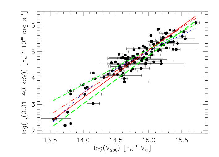
Figure 7.8: Gravitational mass–bolometric X-ray luminosity relation compared to predicted relations. Shown are: best fit relation for the extended sample (solid line), best fit relation determined using HIFLUGCS (triple-dot-dashed line), self similar relation normalized by simulations of Navarro et al., (1995) (dot-dashed line), pre-heated relation given by Evrard and Henry, (1991), using a normalization taken from the simulations of pre-heated clusters by Navarro et al., (1995) (dashed line). The dotted line gives the result of a smoothed spline fit.

In order to compare the empirical $L_{\rm X}$–$M_{\rm tot}$ relation with predictions a quasi bolometric luminosity, $L_{\rm Bol}$, has been calculated in the source rest frame energy range $0.01-40\,{\rm keV}$ (for the relevant range of cluster gas temperatures at least 99 % of the flux is contained in this energy range). In Fig. 7.8 this $L_{\rm Bol}$–$M_{200}$ relation is compared to predicted relations. The solid line shows the best fit relation for the 106 clusters in the extended sample and the triple-dot-dashed line shows the best fit relation determined using HIFLUGCS. Here the bisector fit results have been used in order to treat variables symmetrically, which is the appropriate method for a comparison to theory (e.g., Isobe et al., 1990). The dot-dashed line shows the self similar relation ($L_{\rm Bol}\propto M_{\rm tot}^{4/3}$, Eq. 7.7) normalized by the simulations of Navarro et al., (1995) and the dashed line shows the ‘pre-heated’ relation given by Evrard and Henry, (1991) ($L_{\rm Bol}\propto M_{\rm tot}^{11/6}$, see below), using a normalization taken from the simulations of pre-heated clusters by Navarro et al., (1995). The idea of pre-heating is that the intracluster gas is not cold initially, as in the self similar case, but is heated to a characteristic temperature by some form of non gravitational heat input, e.g., from SNe, early during cluster formation. Assuming the central regions of all clusters to have the same entropy yields the latter relationship. This can be seen by expressing the bolometric luminosity in terms of the central gas density, i.e.

$$L_{\rm Bol}\propto\rho_{\rm gas}(0)^{2-1/\beta}\,T^{1/2}\,M_{\rm tot}$$ (7.10)

(e.g., Evrard and Henry, 1991). If the central specific entropy,

$$s\propto\frac{3}{2}\,k_{\rm B}\,\ln{\frac{T_{\rm gas}}{\rho_{\rm gas}(0)^{\gamma-1}}}\,,$$ (7.11)

is set to a constant value and taking $\gamma=5/3$ one finds

$$\rho_{\rm gas}(0)\propto T_{\rm gas}^{3/2}\,.$$ (7.12)

Plugging this into (7.10) and using $\beta=2/3$, which is close to the mean value in the extended sample, yields

$$L_{\rm Bol}\propto T_{\rm gas}^{5/4}\,M_{\rm tot}\,.$$ (7.13)

With (7.8) one therefore has

$$L_{\rm Bol}\propto M_{\rm tot}^{11/6}\,.$$ (7.14)

Fig. 7.8 shows that measured and predicted relations are in rough agreement, the difference between the predicted relations being larger than the difference to the observed relations. Note, however, that the X-ray luminosity is one of the most uncertain quantities to be derived from simulations. Frenk et al., (1999) recently showed in a comparison of 12 different cosmological hydrodynamics codes that a factor of 2 uncertainty is a realistic estimate of the current accuracy. Including gas cooling in simulations worsens the situation (e.g., Balogh et al., 2001). The slopes of the observed relations are closer to the pre-heated relation. Observationally the effect of pre-heating can also result in a decrease of the gas mass fraction for low temperature systems. This has actually been observed for the clusters in the sample (Sect. 7.4). The possibility that winds from SNe – originally invoked to explain the apparent low gas content of elliptical galaxies (e.g., Mathews and Baker, 1971; Larson, 1974) – pre-heat and dilute the central gas and thereby break the self similarity has been pointed out by various authors (e.g., Kaiser, 1986). Such a process would work most efficiently on the least massive clusters (e.g., White III, 1991; Metzler and Evrard, 1997; Ponman et al., 1999). The spline fit (dotted line in Fig. 7.8) indicates a weak bending, i.e. a slight deviation from a power law, over the entire $M_{200}$ scale. There is some indication that the bend is strongest around $2\times 10^{14}\,h_{50}^{-1}\,M_{\odot}$, suggesting a possible break. In the middle part, where most of the clusters are located, the slope of the dotted line is close to 4/3, while at the low mass end the slope appears even steeper than 11/6.

The Abell catalog (Abell, 1958; Abell et al., 1989), as one of the first and largest systematic cluster catalogs, continues to be a widely used database. The Abell richness (Sect. 2.1.1) has been used frequently in the past as a selection criterium for optical cluster samples (e.g., Colless and Hewett, 1987; Katgert et al., 1996). The construction of the cluster mass function requires a selection closely related to the gravitational cluster mass. The X-ray luminosity has been shown above to exhibit a tight correlation with mass. In Fig. 7.9 the measured number of cluster member galaxies, ${N_{\rm gx}}$, as taken from Abell et al., (1989) is compared to $L_{\rm X}$ as gravitational mass tracer. One notes that there exists a trend for higher mass clusters to have higher values of ${N_{\rm gx}}$. However, there is a huge scatter. One of the main reasons for this poor correlation may be the much less homogeneous background compared to the X-ray case. It is clearly seen that a selection by X-ray luminosity is much more efficient than a selection by Abell richness in terms of mass. Even though only the X-ray surface brightness profile and neither its normalization nor the X-ray luminosity are directly used in the X-ray mass determination via the hydrostatic equation, it is nonetheless reassuring that a similar result is obtained when $L_{\rm X}$ and richness are compared to masses estimated from optical velocity dispersions (Borgani and Guzzo, 2001).

Figure 7.9: Measured number of cluster member galaxies, ${N_{\rm gx}}$, as taken from Abell et al., (1989) and X-ray luminosity of the same (66) clusters as a function of the gravitational mass. Double clusters, whose components have been treated separately here, e.g., A3528n/s, are removed. Above the dashed line all clusters have an Abell richness $R\geq 1$.

Figure 7.10: Mass to light ratio as a function of mass for 18 clusters in common with the sample of Girardi et al., (2000), where the integrated blue band luminosity values within the virial radius have been taken from.

In Fig. 7.10 a plot is shown using a quantity somewhat related to ${N_{\rm gx}}$. Girardi et al., (2000) provide integrated blue band luminosities, ${L_{Bj}}$, within the virial radius. Shown is the mass to light ratio, $M_{200}/{L_{Bj}}$, in units of $h_{50}\,M_{\odot}/L_{\odot}$ (the mass to light ratio of the sun), as a function of $M_{200}$ for the 18 clusters included in the extended sample used here and the $C$ sample of Girardi et al., (2000). One notes that this ratio exhibits a large scatter. Furthermore a very weak trend of a positive correlation with the mass is indicated in agreement with the findings of Girardi et al., (2000). The median mass to light ratio found here equals $103\,h_{50}\,M_{\odot}/L_{\odot}$, implying that the stars in clusters account only for a small fraction of the cluster mass. Taking into account the slight systematic differences in the mass estimates (Sect. 7.2.2) this value agrees with the value quoted by Girardi et al., (2000).

One old and simple technique to estimate the mean density in the universe is to assume this median mass to light ratio to be representative of the universe (see, e.g., Bahcall et al., 1999). If $\Omega_{\rm m}=1$ one would expect $M_{200}/{L_{Bj}}\approx 675\,h_{50}\,M_{\odot}/L_{\odot}$ based on estimates for the total blue band luminosity density (see refs in Girardi et al., 2000). The value found here therefore indicates $\Omega_{\rm m}\approx 0.15$, independent of the Hubble constant. This value should be considered as a rough estimate because of the fairly small number of clusters and the scatter present, because of the difference in the determination of the virial radius for $M_{200}$ and ${L_{Bj}}$, because of the dependence on the accuracy and representativeness of the measured galaxy luminosity functions (which lead to the above mass to light ratio for $\Omega_{\rm m}=1$), and because of the possibility that the mass to light ratio may increase or decrease on even larger scales. Nevertheless the estimate $\Omega_{\rm m}\approx 0.15$ obtained here is in very good agreement with what will be found in Sect. 7.6.2 when the mass function is compared to predictions.

A wide range of possible applications becomes available with the quantification of the $L_{\rm X}$–$M_{\rm tot}$ relation and its scatter. For large X-ray cluster surveys, where individual mass determinations are currently not feasible, luminosities can be directly converted to masses. No combination of observations, simulations, and theory is then needed, like the frequently used approach of relating X-ray luminosities to X-ray temperatures by an observed relation, and converting X-ray temperatures to masses using a relation where the slope is taken from theoretical arguments and the normalization from hydrodynamical simulations (e.g., Moscardini et al., 2000). The observational $L_{\rm X}$–$M_{\rm tot}$ relation has first been applied directly in this sense in the power spectral analysis of REFLEX clusters (Schuecker et al., 2001b ). An example of another direct application is given in Sect. 7.6.3. The $L_{\rm X}$–$M_{\rm tot}$ relation may also be applied to convert theoretical or simulated mass functions to luminosity functions for comparison with observations, which is currently being performed in the interpretation of the REFLEX luminosity function.

At this point it is important to note that even for the highest redshift cluster in the sample used here ($z=0.2$) the dependence of the observational determination of $M_{\rm tot}$ and $L_{\rm X}$ on the chosen cosmological model is very weak. For instance at $z=0.2$ the increase in the luminosity distance, $D_{L}$, and the diameter distance, $D_{A}$, is less than 5 % going from ($\Omega_{\rm m}=1.0,\Omega_{\Lambda}=0$) to ($\Omega_{\rm m}=0.1,\Omega_{\Lambda}=0$). From (2.16) one finds that $M_{\rm tot}(<r)\propto r$ and therefore $M_{\rm tot}(<r)\propto D_{A}$, implying an increase of $M_{\rm tot}$ by less than 5 % for the two models above. For $L_{\rm X}$ one has an increase of less than 10 %. This means that the $L_{\rm X}$–$M_{\rm tot}$ relation given here can be used unchanged for various cosmological applications (unless redshift ranges are probed where evolution becomes important, in this case a model dependent redshift correction has to be introduced). A similar calculation for $V_{\rm max}$ shows that for the extreme case $z_{\rm max}=0.2$ the increase of $V_{\rm max}$ is less than 14 %, which is less than the size of the Poissonian error bars in Fig. 7.14.

More detailed investigations on the shape of the relation and the construction of a volume-limited sample, spanning a reasonably large range in luminosity/mass, to test how much the $L_{\rm X}$–$M_{\rm tot}$ relation given here is affected by being estimated partly from a flux-limited sample are beyond the scope of this work but are envisaged for the future.

7.4 Intracluster Gas Fraction

Even though caused by only 5–6 clusters Figs. 6.2–6.4 clearly suggest a drop in the gas fraction at low cluster masses/temperatures ($\sim 2$ keV). Note, however, that the X-ray emission of the low temperature clusters can in general be traced out to less large (compared to hotter clusters) radii relative to $r_{200}$. Thus more extrapolation is performed rendering the (gas and total) mass estimates more uncertain. On the other hand if the gas mass fraction is indeed significantly lower one would of course just expect to observe emission from the gas less far out. Furthermore, as Vikhlinin et al., (1999) showed, the gas density profile steepens ($\beta$ increases) only slightly in the outer cluster parts and they concluded that mass estimates are not significantly affected. Nevertheless a possibly underestimated $\beta$ value for the low temperature clusters would rather lead to an overestimated value for $f_{\rm gas}$ (Eq. 7.15 and Fig. 7.11), which indicates that the low gas fractions for the low $T_{\rm X}$ systems found here are not an artefact. In any case deeper observations of low temperature clusters are needed to resolve this issue. Despite the problems of a high background level (Chap. 5), XMM-Newton with its large effective area seems currently to be best suited for this purpose.

The importance of more and especially deeper observations becomes even more obvious when the results from other works are compared. David et al., (1995) showed for a sample of 11 clusters that $f_{\rm gas}$ increases continuously between ellipticals, groups, and clusters. The analysis by Evrard, (1997), who combined $f_{\rm gas}$ measurements from White and Fabian, (1995) and David et al., (1995) ($1\lesssim T_{\rm X}\lesssim 14$ keV), showed that a homogeneously analyzed cluster sample is vital if trends in the gas fraction are to be studied. First a trend of decreasing $f_{\rm gas}$ with increasing $T_{\rm X}$ was indicated, but after the cluster gravitational masses had been homogeneously redetermined this trend disappeared. Allen and Fabian, (1998) found that $f_{\rm gas}$ is decreasing with increasing $T_{\rm X}$ for a sample of 30 high luminosity clusters after they had corrected the temperatures for cooling flows. However, their sample contains rather hot clusters mainly (5.5–26.4 keV). Ettori and Fabian, (1999) found no statistically significant dependence of $f_{\rm gas}$ on $M_{\rm tot}$ or $T_{\rm X}$ for a sample of 36 high luminosity clusters once the sample was corrected for a redshift dependence. When the redshift dependence was neglected they found results in agreement with Allen and Fabian, (1998). Arnaud and Evrard, (1999) found indications for an increase of $f_{\rm gas}$ with increasing $M_{\rm tot}$ using a sample of 24 clusters in the range $2.2\leq T_{\rm X}\leq 14.6$ keV. Mohr et al., (1999) found a trend of increasing $f_{\rm gas}$ with increasing $T_{\rm X}$ for a sample of 45 galaxy clusters ranging in $T_{\rm X}$ from 2.4 to 10.1 keV. Roussel et al., (2000) analyzed 33 clusters in the temperature range 1–14 keV and found no clear trend of $f_{\rm gas}$ with $T_{\rm X}$. Grego et al., (2001), who determined the shape of the gas density profile utilizing interferometric measurements of the Sunyaev–Zeldovich effect, found no indication for a dependence of $f_{\rm gas}$ on $T_{\rm X}$ for a sample of 18 galaxy clusters. Their sample includes only rather hot (5.7–13.2 keV) clusters, however, whereas the effect appears to be strongest for cool clusters.

It is worth noting that while David et al., (1995) found that the gas fraction comprises only a few percent of the total mass in ellipticals and small groups, David, (1997), inspired by the early findings that a large fraction of the galactic mass may be in the form of massive compact halo objects (MACHOs; Alcock et al., 1997), argued that the total baryon fraction may actually stay constant at about 50 % independent of mass scale (from ellipticals to rich clusters) if MACHOs mainly consisted of stellar remnants (e.g., Fields et al., 1997; Alcock et al., 1997), e.g., white dwarfs, which would also explain the abundance of heavy elements in the intergalactic medium. However, the galactic halo mass fraction contained in MACHOs has been significantly reduced recently (Alcock et al., 2000). David et al., (1990) and David, (1997) also showed that the ratio gas mass over stellar mass increases with gas temperature, confirmed by Arnaud et al., (1992) who found the same trend with cluster richness. Roussel et al., (2000), however, did not find strong evidence of an increase of this ratio with $T_{\rm X}$. The main part of the discrepancy seems to arise from the fact that Roussel et al., (2000) did not find an increase of $f_{\rm gas}$ with $T_{\rm X}$. As mentioned later in more detail Bryan, (2000) compiled evidence for not only an increase of $f_{\rm gas}$ with $T_{\rm X}$ but also for a decrease of the mass fraction contained in stars with increasing $T_{\rm X}$.

In summary it is concluded that the large spanned temperature range available in this work has allowed to find that the gas mass fraction A) does not vary systematically for clusters with $T_{\rm X}\gtrsim 2$ keV and B) drops abruptly for groups and clusters with lower gas temperatures in agreement with some of the previous works. The fact that the X-ray extent relative to the virial radius is usually smaller for groups than for clusters may be interpreted as a consequence of the lower gas fraction. Since proposed scenarios to explain a systematic variation of the gas fraction with temperature or mass, e.g., pre-heating, should be considered also in the light of relations between other cluster parameters, they are further discussed in Sect. 7.5.

In Fig. 6.5 it has been shown that for most clusters the gas mass fraction appears to vary with radius. For the majority of those clusters $f_{\rm gas}$ seems to increase with radius, i.e. between $r_{500}$ and $r_{200}$. There appears to be no significant trend of this variation with system mass for the low to medium mass clusters. However, the gas fraction apparently becomes more likely to increase less fast or decrease with radius for the massive clusters. How may this be understood? Since $\beta$ is an important parameter both for the gas and gravitational mass determination let us first estimate the behavior of $f_{\rm gas}$ as a function of $\beta$. Dividing (2.3) by (2.16) one gets an approximate expression for the gas fraction

$$f_{\rm gas}(<r)\approx f(T_{\rm gas},\rho_{\rm gas}(0),\beta,r_{\rm c})\left(\frac{r}{r_{\rm c}}\right)^{-3\beta+2}\quad:\quad\frac{r}{r_{\rm c}}\gg 1\wedge\beta<1\,,$$ (7.15)

where the intracluster gas has been assumed in hydrostatic equilibrium and isothermal. Therefore one has by construction an increasing gas fraction with increasing radius for $\beta\lesssim 2/3$ and a decreasing gas fraction for $\beta\gtrsim 2/3$. This is illustrated more precisely (keeping only the latter two assumptions for the intracluster gas) in Fig. 7.11 for some typical parameter values. It is worth noting that from this Figure it is also clear that the gas fraction rises with radius out to $\gtrsim 5\,r_{\rm c}$ as long as $\beta\lesssim 0.8$, i.e. for most of the clusters. Plotting the gas fraction ratios as determined for the clusters in this work as a function of the observed $\beta$ values (Fig. 7.12) confirms the decrease of $f_{\rm gas}$ with increasing radius in the outer cluster parts for $\beta\gtrsim 2/3$.

Figure 7.11: Radial variation of the gas fraction. Solid line: $\beta=2/3$, dashed line: $\beta=0.8$, dot-dashed line: $\beta=0.5$. $r_{\rm c}=150$ kpc, $k_{\rm B}T_{\rm gas}=5$ keV, $n_{\rm e}(0)=0.01\,\rm cm^{-3}$.

Figure 7.12: Variation of the gas fraction as a function of $\beta$. Error bars have been omitted.

As expected therefore $\beta$ is the relevant parameter here. The variation of $\beta$ as a function of mass therefore determines the variation of $f_{{\rm gas},200}/f_{{\rm gas},500}$ with mass. A quick look to Fig. 6.9 confirms this. So also trends of the radial variation of the gas mass fraction need to be discussed in the context of other relations, which is done in the next Section.

7.5 Relations between Shape Parameters, Temperature, Luminosity, and Mass

In this Section the relations found in Sect. 6.3 are discussed. Suggested models to explain the observed behavior – including the variation of the gas mass fraction – are described. It is discussed whether the predictions of a single scenario fit all relations.

It has long been known that a correlation exists between $L_{\rm X}$ and $T_{\rm X}$ (e.g., Mitchell et al., 1977). Most authors find best fit relations similar to $L_{\rm Bol}\propto T_{\rm X}^{3}$, as has been found here, too. This is significantly steeper than the simple self similar prediction $L_{\rm Bol}\propto T_{\rm X}^{2}$. Note that inclusion of line emission – more important for cooler systems– would further flatten this relation.

In principle a dependence of the gas fraction on temperature could account for a steeper $L_{\rm Bol}$–$T_{\rm X}$ relation (Eq. 7.9). And really it has been found in Sect. 6.2 that the gas fraction increases with increasing temperature. But this is true only for the lowest temperature clusters (Fig. 6.4). So clearly this trend of the gas fraction cannot account for the steepness of the $L_{\rm X}$–$T_{\rm X}$ relation over the entire $T_{\rm X}$ range.

In addition to this deviation from self similarity over the entire $T_{\rm X}$ range, interestingly some authors have found a bend in the $L_{\rm X}$–$T_{\rm X}$ relation in the sense that low $T_{\rm X}$ clusters give rise to an even steeper $L_{\rm X}$–$T_{\rm X}$ relation (e.g., Helsdon and Ponman, 2000). Other authors find no evidence for such a feature (e.g., Mulchaey and Zabludoff, 1998). In this work there is also no clear indication of any bend ranging from 0.7–13.3 keV.

The $M_{\rm tot}$–$T_{\rm X}$ relation has in general been found observationally to be steeper than the self similar prediction $M_{\rm tot}\propto T_{\rm gas}^{3/2}$ (Eq. 7.8) and the normalization has been found by previous authors to be lower than the normalization expected from simulations (e.g., Finoguenov et al., 2001, and references therein). Both trends are seen here, too, indicating that the interpretation of temperature functions in a cosmological context depends systematically on the used method for the conversion between $T_{\rm X}$ and $M_{\rm tot}$, in agreement with the findings of, e.g., Ikebe et al., (2001). Furthermore no clear deviation from a power law is found here. Note that $T_{\rm gas}$ is needed for the calculation of $M_{\rm tot}$ (Eq. 2.16). These two quantities are therefore not determined independently of one another.

A possible dependence of the gas density profile, i.e. of the shape parameter $\beta$, on temperature has been indicated by observations of previous authors (e.g., David et al., 1990; White III, 1991; Mohr and Evrard, 1997; Arnaud and Evrard, 1999; Jones and Forman, 1999; Lloyd-Davies et al., 2000; Helsdon and Ponman, 2000). However, e.g., Mohr et al., (1999), Vikhlinin et al., (1999), and Roussel et al., (2000) have found no clear or only a weak trend. Fig. 6.10 shows that for the 88 clusters with measured temperature analyzed in this work there is no trend found, especially not at the low temperature side. There may be indications of increasing $\beta$ values with increasing $T_{\rm X}$ at the high temperature side, but the evidence is only weak. Stronger indications indeed are found if $\beta$ is plotted as a function of gravitational mass (at the high mass side). Interpretations of this apparent trend, however, must be taken cautiously since $\beta$ enters the calculation of $M_{\rm tot}$ (Eq. 2.16). There are two effects which are likely to enhance the very weak trend seen in Fig. 6.10 as compared to Fig. 6.9. First of all $M_{200}\propto T_{\rm X}^{1.65\pm 0.05}$ (Tab. 6.11) and therefore a possible trend with $M_{200}$ will appear weaker in $T_{\rm X}$. Secondly, the temperatures of the clusters with higher $\beta$ values at around 4–6 keV (causing the slight bumb in the spline fit) are translated into relatively higher masses (Eq. 2.16).

The trend of $\beta$ at high masses may be understood by considering that the core radius clearly correlates with gravitational mass (Fig. 6.8, even though a large mass range is needed to detect this correlation due to substantial scatter). For large core radii $\beta$ increases with increasing $r_{\rm c}$ (Fig. 6.6). It is therefore not surprising that for large masses $\beta$ increases with increasing mass.

A tight correlation exists between the gas mass and the gas temperature (Fig. 6.13). The lowest temperature clusters have gas masses below the prediction by the best fit relation. This is consistent with the finding that the gas mass fraction drops suddenly for the lowest $T_{\rm X}$ clusters. A similar behavior, though less obvious, is seen in Fig. 6.12: low luminosity clusters have a smaller gas mass then expected from the best fit relation.

As outlined above and in the previous Section measurements by different authors show different strengths of deviations from expected relations. This is obviously due to the fact that the measurements are difficult and several effects may lead to slight distortions of the results. Some of the main problems are summarized here. For low temperature clusters the gas is traced out least far relative to the virial radius, which affects the uncertainty of almost all measured quantities. Combination of heterogeneous samples, e.g., poor groups from author X combined with rich clusters analyzed by author Y, may introduce artificial trends. Purely X-ray flux-limited samples may be less (or more) sensitive to deviations in relations compared to volume-limited samples (which are currently difficult to assemble with the necessary quality and size), especially when the X-ray luminosity is involved. The presence of central excess emission may bias the determination of the fit parameter values in the sense that a too small core radius and therefore possibly a too small $\beta$ value is measured (e.g., Mohr et al., 1999). This effect, if present, seems not to bias the determination of the gas mass, however, as has been shown by comparison of gas masses determined with single and double $\beta$ models (e.g., Reiprich, 1998). Since the excess emission is often connected with a drop in temperature towards the very center, overall temperatures may be biased low if this effect is not taken into account (e.g., Chap. 5; for more subtle effects on temperature estimates due to accretion of small cool clumps of gas see Mathiesen and Evrard, 2001). On the other hand the presence of substructure may increase the temperature, the core radius and therefore possibly also $\beta$ (e.g., Jones and Forman, 1999, but see Neumann and Arnaud, 1999). Mass estimates based on the hydrostatic assumption are also uncertain in major mergers and additionally the X-ray luminosity may be strongly affected, at least for a short time (e.g., Ricker and Sarazin, 2001). A possible dependence of the surface brightness profile and gas temperature determination on the covered energy range may introduce artificial systematic trends, e.g., between $\beta$ and $T_{\rm X}$. If the gas temperature depends on radius in the outer parts, the assumption of isothermality leads to a biased mass estimate (Sect. 7.2.1, see also Chap. 5). The contribution of line emission becomes non negligible for low $T_{\rm X}$ clusters (e.g., Böhringer and Hensler, 1989), therefore deviations from the simplest self similar relations (assuming pure bremsstrahlung emission) are expected even if clusters were self similar. As a consequence also possible metallicity variations between groups and clusters (Davis et al., 1999 for instance find lower metallicities for low $T_{\rm X}$ groups) may affect the group luminosities if typical cluster metallicities are assumed. Note that the deviations from the self similar relations are at least partly rather small, e.g., in the case of the $M_{\rm tot}$–$T_{\rm gas}$ relation, therefore it is necessary to be aware even of the partially probably small effects that have just been outlined. However, they are not likely to strongly distort the results obtained from the mass function and some of the realistic possibilities have explicitly been shown to cause only deviations smaller than the statistical uncertainty, e.g., the possible presence of strong gradients in the gas temperature (Sect. 7.6.2).

Accordingly a wide variety of models has been suggested to explain the observations. The currently most popular models concern heating. This heating may have occured universally prior to the assembly of groups, just before, during or after collapse (e.g., Wu et al., 1998a ; Valageas and Silk, 1999; Loewenstein, 2000; Kravtsov and Yepes, 2000; Wu et al., 2000; Tozzi and Norman, 2001; Brighenti and Mathews, 2001; Wu et al., 2001b ; Bower et al., 2001). Since the required energy input depends on the gas density at the time of injection and the assumed fraction of the released energy that goes into gas heating, the cited amounts vary by an order of magnitude from 0.1–0.3 to 1–3 keV/particle. Various heat sources have been suggested. Among them SNe, AGN, and population III stars.

But also other mechanisms have been proposed. For instance Muanwong et al., (2001) find in simulations that cooling of the intracluster gas alone may account for observed deviations, due to removal of low entropy gas. Based on some evidence (compiled from Mulchaey et al., 1996, Hwang et al., 1999, and Cirimele et al., 1997) that while the gas fraction in clusters decreases with decreasing temperature the mass fraction in stars increases (but see, e.g., Roussel et al., 2000, who do not find a similar trend), Bryan, (2000) shows that a higher efficiency of galaxy formation in groups compared to clusters (e.g., David et al., 1990) suffices to explain observations without the need of additional heating. A comparison of the predictions of this model to indications for a metallicity decrease in low temperature groups (e.g., Davis et al., 1999) may be interesting.

Mathiesen et al., (1999) investigated the effects of clumping and substructure on measurements of $M_{\rm gas}$. Using an ensemble of 48 simulated clusters they measured a mean mass weighted clumping factor $C\equiv\langle\rho_{\rm gas}^{2}\rangle/\langle\rho_{\rm gas}\rangle^{2}\approx$ 1.3–1.4 within $r_{500}$. They showed that $\langle M_{\rm gas}^{\rm measured}/M_{\rm gas}^{\rm true}\rangle\approx\sqrt{C}$, indicating that gas masses estimated assuming a uniform density profile at a given radius overestimate the true gas mass by about 16 %, which is of the same order as the statistical uncertainties in this work ($\langle\Delta M_{{\rm gas},500}/M_{{\rm gas},500}\rangle=15\,\%$). Furthermore they found no trend with cluster bulk properties like temperature or mass. The possibility of scale dependent clumping therefore seems to be excluded as causing deviations from self similar relations. They showed further that the presence of moderate substructure does not bias the gas mass measurements significantly.

A synopsis of the main trends indicated from the relations presented in this work is now given. The gas fraction seems to be constant for $T_{\rm X}\gtrsim 2$ keV. For lower temperatures a steep decrease of $f_{\rm gas}$ is indicated. A straightforward conclusion is that smaller systems contain comparatively less gas. At the same time there are no indications for a flattening of the gas density profile for these groups. Neither $\beta$ becomes smaller, that is no flattening of the surface brightness profile in the outer part is observed (at least out to $r_{\rm X}$), nor does $r_{\rm c}$ become larger, that is no flattening in the very central regions is observed. The observed $L_{\rm X}$–$T_{\rm X}$ and $M_{\rm tot}$–$T_{\rm X}$ relations are steeper than the self similar expectation over the entire $T_{\rm X}$ range, whereas variations in $f_{\rm gas}$ seem to occur only at low temperatures. It is therefore not necessarily clear that these deviations (observed at different scales) are caused by one and the same physical process.

Heating of the ICG must have occured at some point as evidenced by the observed metallicities. It is possible that the energy provided by SNe is sufficient to account for the decrease in the gas mass fraction for the lowest temperature systems, but possibly does not suffice to steepen the $L_{\rm X}$–$T_{\rm X}$ and $M_{\rm tot}$–$T_{\rm X}$ relations over the entire $T_{\rm X}$ range (e.g., Wu et al., 2000). A flatter gas density profile for low temperature clusters as one might expect in this scenario is not observed here. The steeper slope and lower normalization of the $M_{\rm tot}$–$T_{\rm X}$ relation may be caused by an increase in average formation redshift for decreasing system mass (e.g., Finoguenov et al., 2001), i.e. by hierarchical growth of structure. Since in this case low mass systems would have formed in a higher density environment this implies comparatively higher temperatures (and smaller core radii, in agreement with the steep relation between $r_{\rm c}$ and $T_{\rm X}$ observed here). However, neglecting cooling this effect would also increase the luminosity on average for lower temperature systems thereby tending to cause a flattening of the $L_{\rm X}$–$T_{\rm X}$ relation. Since the emissivity depends on the density squared cooling may be more important for systems formed in a higher density environment resulting in a more efficient removal of gas and therefore a larger decrease in luminosity in line with observations. In this work no attempt has been made to model or simulate these effects in detail, but the aim has rather been to determine observationally relevant relations in a homogeneous way for a cluster sample not dominated by subjective selection criteria for a large temperature interval and describe possible scenarios accounting for them. Even though the overall physical processes determining the main observational appearance of galaxy clusters are well understood, at the moment it seems unclear which effect contributes most to the observed deviations from self similarity. It appears unlikely that a single suggested effect can account for all of them.

7.6 Mass Function

This Section starts out with a comparison of the mass function determined here with previous determinations. In Sect. 7.6.2 constraints on cosmological parameters are derived. And in Sect. 7.6.3 the $L_{\rm X}$–$M_{\rm tot}$ relation is applied to convert a luminosity function into a ‘mass’ function as an example.

7.6.1 Comparison to Previous Estimates

Bahcall and Cen, (1993) give a mass function constructed a) from optically selected clusters with masses determined from the galaxy richness and b) from the cluster X-ray temperature function given by Henry and Arnaud, (1991). Very good agreement is found for masses determined within $r_{\rm A}$ between the Bahcall and Cen, and the HIFLUGCS mass function (Fig. 7.13).

Figure 7.13: Cumulative gravitational mass function for HIFLUGCS using three different outer radii. Vertical error bars give the Poissonian errors. Horizontal bars indicate the individual bin sizes. Each bin contains 10 clusters, apart from the highest mass bin, which contains 13 clusters. The abundances from previous works are determined for $M_{\rm A}$.

White et al., 1993a constrain the cluster abundance by using published values for the abundance and median velocity dispersion of richness class $R\geq 1$ Abell clusters. It is not surprising that their density is significantly higher than the HIFLUGCS density since they intentionally use conservative mass estimates, which are overestimates of the true cluster mass.

Biviano et al., (1993) and Girardi et al., 1998a have determined the cluster mass function using optically selected cluster samples with masses determined from published line-of-sight velocity dispersions of cluster galaxies. At the completeness limit given by Girardi et al., 1998a (, triangle in Fig. 7.13) the cluster density given by Biviano et al., (1993) is about a factor of two higher than the density given by Girardi et al., 1998a . The latter authors explain this difference in density by their on average 40 % smaller mass estimates due to an improved technique for removing interlopers and the use of a surface-correction term in the virial theorem compared to Biviano et al., (1993). The value given by Girardi et al., 1998a itself lies significantly higher than the comparable HIFLUGCS density. The reason could lie in the fact that their optically estimated masses are on average slightly larger than the X-ray masses or that the external normalization for $R\geq 1$ (${N_{\rm gx}}\geq 50$) clusters which they applied to their mass function is intrinsically higher than the normalization obtained through HIFLUGCS directly, or both. In Sect. 7.2.2 it has been found that for a common subsample of 42 clusters the virial masses determined by Girardi et al., 1998a are on average 25 % larger than the masses determined in this work. This difference might be smaller if masses out to the Abell radius were compared, since common radii would be used in this case. Increasing the X-ray masses artificially by 25 %, the diamonds in Fig. 7.13 shift towards higher masses, but the shift is too small to account for the difference to the triangle. The large scatter in the ${N_{\rm gx}}$–$M_{\rm tot}$ diagram (Fig. 7.9) makes a reliable estimate of a best fit relation between these two quantities very difficult. Nevertheless, in order to get a rough idea of the mass within $r_{\rm A}$ that corresponds to ${N_{\rm gx}}=50$, I have performed fits using the minimization methods outlined earlier and find $5.1\lesssim M_{\rm A}({N_{\rm gx}}=50)\lesssim 8.8\times 10^{14}\,h_{50}^{-1}\,M_{\odot}$. Note that this range is in agreement with the ranges $5$–$8\times 10^{14}\,h_{50}^{-1}\,M_{\odot}$ and $5$–$7\times 10^{14}\,h_{50}^{-1}\,M_{\odot}$ given by Bahcall and Cen, (1993) and Girardi et al., 1998a , respectively, for $N_{\rm gx}=50$. This mass range corresponds to a cumulative number density obtained through HIFLUGCS in the range $1.7\lesssim n(>M_{\rm A})\lesssim 8.7\times 10^{-7}\,h_{50}^{3}\,\rm Mpc^{-3}$. The external density estimate applied to normalize the Girardi et al., 1998a mass function therefore is a factor 1.2–6.2 higher than the corresponding estimate obtained here. It is therefore concluded that both effects (masses and normalization) are important but the latter factor is responsible for a larger fraction of the discrepancy. Assuming both normalizations to be determined from samples that are highly complete and representative of the local universe this may indicate that either X-ray and optical clusters are drawn from different populations or that projection effects (e.g., line of sight galaxy overdensities, which do not form a bound structure in three dimensions) possibly bias optically determined normalizations high.

Girardi and Giuricin, (2000) recently extended the mass function to loose galaxy groups, finding $n(>1.8\times 10^{13}\,h_{50}^{-1}\,M_{\odot})=1.6$–$2.4\times 10^{-4}\,h_{50}^{3}\,\rm Mpc^{-3}$, which is outside the mass range that can be tested here. They find that the group mass function can be described by a smooth extension of the cluster mass function by Girardi et al., 1998a . Consistently this abundance is higher than the abundance given by Bahcall and Cen, (1993) at that mass scale.

Carlberg et al., (1997) have compiled and partially reestimated abundances for local cluster samples (Henry and Arnaud, 1991; Mazure et al., 1996; White et al., 1993a ; Eke et al., 1996) for comparison with higher redshift samples (the ‘$\times$’ shows the density for a sample with higher mean redshift and therefore it cannot be compared directly). In general the comparison to the HIFLUGCS mass function shows better agreement than the abundances given by Girardi et al., 1998a and White et al., 1993a .

The obvious importance of the definition of the cluster outer radius for the cluster mass function can be directly appreciated by noting the large differences between the mass functions determined for HIFLUGCS for $M_{500}$, $M_{200}$, and $M_{\rm A}$ in Fig. 7.13, especially towards lower masses. Since for self similar clusters the mass scales with the third power of the characteristic radius (Sect. 7.3), determination of the mass within a characteristic overdensity is the natural choice. The formally determined $M_{\rm A}$ mass function is mainly given for the comparison with previous mass functions and it is recalled again that especially for the low mass systems the assumption of hydrostatic equilibrium may not be justified out to $r_{\rm A}$, and therefore the mass estimates for $M_{500}$ and $M_{200}$ should be considered much more precise than the estimates for $M_{\rm A}$. Note that it also seems likely that especially small clusters and groups are not in virial equilibrium out to $r_{\rm A}$.

7.6.2 Comparison to Predicted Mass Functions

In this Section one of the main results of this work is derived and discussed. The mean density of the universe is determined by a comparison of the observed and predicted mass function. The formalism outlined in Sect. 2.2.3.2 is used for the calculation of mass functions for given cosmological models. As mentioned earlier due to the low redshift range spanned by HIFLUGCS, the effect of a redshift correction is very small and therefore $z=0$ is set for all calculations, unless noted otherwise.

Similarly to the work of Ikebe et al., (2001) the statistical uncertainty in the mass determination is incorporated in the model mass function as

$$\frac{d\tilde{n}(M)}{dM}\equiv\frac{1}{V_{\rm max}(M)}\,\int^{\infty}_{-\infty}\frac{dn(M^{\prime})}{dM^{\prime}}\,V_{\rm max}(M^{\prime})\,$$

$$\times\,(2\pi\,\bar{\sigma}_{M_{\rm tot},\log}^{2})^{-1/2}\,\exp\left(\frac{-(\log M^{\prime}-\log M)^{2}}{2\,\bar{\sigma}_{M_{\rm tot},\log}^{2}}\right)d\log M^{\prime}\,,$$ (7.16)

where $\bar{\sigma}_{M_{\rm tot},\log}=0.12$ represents the logarithmic mean mass measurement uncertainty. Note that since HIFLUGCS is flux-limited and not volume-limited the weighting has to be performed on the mass distribution, $N(M)/dM$, rather than on the mass function itself. The effect of this weighting on the model mass function is a slight amplitude increase at the high mass end.

For the modeling to be independent of the precise knowledge of the $L_{\rm X}$–$M_{\rm tot}$ relation the quantitative comparison has been performed using a standard $\chi^{2}$ procedure on the differential binned mass function given in Fig. 7.14 (rather than using a maximum likelihood approach on the mass distribution). The $\chi^{2}$ values have been calculated in a fine grid of $\Omega_{\rm m}$ and $\sigma_{8}$ values assuming a flat cosmic geometry. The cosmological constant enters the calculation only through $\delta_{\rm c}$ and therefore has a negligible influence here. The minimum and statistical error ellipses for some standard confidence levels (c.l.) are given in Fig. 7.15. The tight constraints obtained show that with HIFLUGCS one can go beyond determining an $\Omega_{\rm m}$–$\sigma_{8}$ relation and put limits on $\Omega_{\rm m}$ and $\sigma_{8}$ individually. It is found that

$$\Omega_{\rm m}=0.12^{+0.06}_{-0.04}\quad{\rm and}\quad\sigma_{8}=0.96^{+0.15}_{-0.12}$$ (7.17)

(90 % c.l. statistical errors for two interesting parameters), indicating a relatively low value for the density parameter. The large covered mass range and the specific region in $\Omega_{\rm m}$/$\sigma_{8}$ parameter space allow to derive these tight constraints from a local cluster sample. For comparison for a given $\sigma_{8}$ value the $\Omega_{\rm m}$ value which minimizes $\chi^{2}$ is calculated. These pairs can then roughly be described by a straight line in log space given by (using the usual notation)

$$\sigma_{8}=0.43\,\Omega_{\rm m}^{-0.38}\,.$$ (7.18)

In Fig. 7.14 also the best fit model mass functions for given $\Omega_{\rm m}=0.5$ and $\Omega_{\rm m}=1.0$ are plotted and one notes immediately that these value pairs give a poorer description of the shape of the mass function. Previous estimates have generally yielded a combination of slightly higher $\Omega_{\rm m}$/$\sigma_{8}$ values (e.g., Peacock, 1999, Sect. 17.2). It has to be noted, however, that for instance in the important work of White et al., 1993a , who find $\sigma_{8}\approx 0.57\,\Omega_{\rm m}^{-0.56}$, the authors explicitly state that their estimates of $\sigma_{8}$ are probably biased high due to their conservative mass estimates.

Figure 7.14: HIFLUGCS mass function compared to the best fit model mass function with $\Omega_{\rm m}=0.12$ and $\sigma_{8}=0.96$ (solid line). Also shown are the best fit model mass functions for fixed $\Omega_{\rm m}=0.5$ ($\Rightarrow\sigma_{8}=0.56$, dashed line) and $\Omega_{\rm m}=1.0$ ($\Rightarrow\sigma_{8}=0.43$, dotted line).

Due to the large given ranges of several orders of magnitude in mass and especially density the $\chi^{2}$ values have been determined from comparison model/data naturally in log space. However, it has been verified that the same calculation in linear space yields best fit values lying within the 68 % error ellipse.

In Sect. 6.4 arguments have been given why $V_{\rm max}(L_{\rm X})$ has been used for the determination of the mass function. Nevertheless if $V_{\rm max}(M_{\rm tot})$ is used instead (see Fig. 6.15), consistent results are obtained. Since in this case one wants to estimate $L$ from $M$ the relation ($L\mid M$) is the appropriate one (e.g., Isobe et al., 1990). Performing a fit to a mass function constructed with $V_{\rm max}(M_{\rm tot})$ results in best fit values $\Omega_{\rm m}=0.14$ and $\sigma_{8}=0.86$, which is consistent with the error range given in (7.17).

As shown in Sect. 7.2.1 it is possible that the assumption of isothermality leads to an overestimate of the cluster masses on average. Therefore the robustness of the results has been tested by multiplying the isothermal cluster masses by 0.799 and recalculating the minimum. As expected values for both $\Omega_{\rm m}$ and $\sigma_{8}$ are found to be lower. But the new minimum is contained well within the error ranges given in (7.17). On the other hand in Sect. 7.2.2 it has been shown by comparison with optical mass measurements that masses could possibly be underestimated. After increasing all cluster masses by 25 % a fit shows that both $\Omega_{\rm m}$ and $\sigma_{8}$ become slightly larger, but again they lie well within the range (7.17). Therefore these tests indicate that the constraints obtained here are fairly insensitive against systematic uncertainties in the mass measurements.

As mentioned in Sect. 4.2 it has been shown that the small range of low redshifts covered here ensures that no redshift corrections need to be applied. Nevertheless it has been tested whether or not the best fit parameter values change if $M_{200}$ is calculated using $\rho_{\rm c}=\rho_{\rm c}(z)$ for the extreme (strong evolution) case ($\Omega_{\rm m}=1,\Omega_{\Lambda}=0$), i.e. $\rho_{\rm c}=4.6975\times 10^{-30}\,(z+1)^{3}\,\rm g\,cm^{-3}$ for each cluster redshift (Eqs. 2.32 and 2.40). The model mass function is then calculated for the mean redshift of HIFLUGCS, $\langle z\rangle=0.05$, using the formulae outlined in Sect. 2.2.3.2. It has been found that within the grid used here the best fit values do not change at all and also the error ellipses are almost not affected, thereby confirming that the application of redshift corrections does not affect the results.

The value $H_{0}=71\,\rm km\,s^{-1}\,Mpc^{-1}$ has been adopted for the calculation of model mass functions based on the recent combination of constraints obtained using the Hubble Space Telescope (Mould et al., 2000). Setting the Hubble constant to their lower limit, $H_{0}=65\,\rm km\,s^{-1}\,Mpc^{-1}$, does not affect the best fit parameter values significantly. Using even $H_{0}=60\,\rm km\,s^{-1}\,Mpc^{-1}$ changes the results for $\Omega_{\rm m}$ and $\sigma_{8}$ only well within the 68 % error ellipse. Therefore the constraints obtained here on these cosmological parameters do not depend significantly on the specific choice of $H_{0}$.

The data point in Fig. 7.14 that may be affected most by cosmic variance is the one at the lowest mass, since the maximum search volume is smallest for the clusters in this bin. Therefore the sensitivity of the best fit results on this last point has been tested by ignoring it. The decrease in the covered mass range of course increases the resulting error ellipse, but the best fit values vary only within the (smaller) 68 % error ellipse. It may be worth noting that leaving out the highest mass bin or leaving out the highest and lowest mass bin changes the best fit values only within the 90 % error ellipse.

Since it has been found that for the estimate of the statistical errors one needs to explore ranges $\Omega_{\rm m}<0.1$ for $\Omega_{\rm b}\sim 0.04$ I regarded it necessary to check if the approximation to the transfer function as given in Sect. 2.2.3.2 is still applicable. Recently Eisenstein and Hu, (1998) derived a fitting function, that includes, e.g., also the oscillations induced by the baryons, which gives a better description of transfer functions computed with CMBFAST (Seljak and Zaldarriaga, 1996) than fitting functions for zero or small baryon contribution to the total matter density derived previously. Therefore this improved version of an analytic transfer function has been incorporated in the $\chi^{2}$ procedure. It has been found that within the used grid the minimum does not change at all, the choice of the Bardeen et al., (1986) fitting function combined with the shape parameter given by Sugiyama, (1995) therefore seems to be accurate enough for the purposes here. However, the confidence contours towards low $\Omega_{\rm m}$ are getting compressed when the Eisenstein and Hu, (1998) fitting function is used, thereby slightly decreasing the area of the error ellipse for a given confidence level. Since the latter statistical error ellipse can be regarded as more realistic, this one is shown in Fig. 7.15.

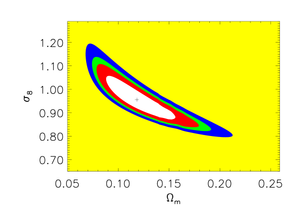
Figure 7.15: Statistical confidence contours for the $\chi^{2}$ procedure. The cross indicates the minimum. Ellipses indicate 68 %, 90 %, 95 %, and 99 % confidence levels for two interesting parameters.

It has also been tested whether or not the recently found deviations of the PS formalism compared to large $N$-body simulations (e.g., Governato et al., 1999; Jenkins et al., 2001) have a significant influence on the results obtained here. The best fit PS model ($\Omega_{\rm m}=0.12$, $\sigma_{8}=0.96$) has been compared to the model obtained using the ‘universal’ mass function (fit to $N$-body simulations, Jenkins et al., 2001) for the same parameter values. These two models agree well for $M\lesssim 10^{15}\,h_{50}^{-1}\,M_{\odot}$. The differences become larger than the size of the Poissonian error bars (Fig. 7.14) for $M\gtrsim 2\times 10^{15}\,h_{50}^{-1}\,M_{\odot}$, in the sense that the Jenkins et al., mass function predicts higher cluster abundances than PS. For larger values of $\Omega_{\rm m}$ the differences become comparable to the size of the error bars at lower masses, e.g., for $\Omega_{\rm m}=\sigma_{8}=0.5$ around $M\sim 5\times 10^{14}\,h_{50}^{-1}\,M_{\odot}$. To estimate the influence of these differences on the best fit values derived using the PS mass function, the parameter values of the Jenkins et al., model have been adjusted to reproduce the PS mass function, where $\Omega_{\rm m}=0.15$ and $\sigma_{8}=0.86$ have been found. The value for $\Omega_{\rm m}$ becomes slightly larger but the combination of both values is still contained within the 90 % error ellipse. It is therefore concluded that the differences between the model mass functions do not significantly affect the interpretation of the HIFLUGCS mass function. Moreover this test can be regarded as confirmation of the validity of the PS mass function for the accuracy needed here.

Also in this work the normalized baryon density may be estimated, using the mean gas mass fraction determined in Sect. 6.2. One may set the gas mass fraction in clusters, being the largest collapsed objects, equal to the baryon fraction in the universe, i.e. $f_{\rm gas}=\Omega_{\rm b}/\Omega_{\rm m}$. It has been tested if consistent results are obtained if the value determined for $\Omega_{\rm b}$ here is used for the calculation of model mass functions instead the one given in Sect. 2.2.3.2. Using $\Omega_{\rm b}=0.19\pm 0.08\,h_{50}^{-3/2}\,\Omega_{\rm m}$ results in model mass functions very similar to the ones calculated using the baryon fraction given by Burles and Tytler, (1998). It is therefore not surprising that the best fit values for $\Omega_{\rm m}$ and $\sigma_{8}$ vary only well within the 68 % error ellipse if the former $\Omega_{\rm b}$ determination is used.

It is worth noting that combining these two measurements of $\Omega_{\rm b}$, i.e. $0.19\pm 0.08\,h_{50}^{-3/2}\,\Omega_{\rm m}=0.0772\,h_{50}^{-2}$, gives further evidence for a low value for $\Omega_{\rm m}$ by yielding an estimate $\Omega_{\rm m}=0.34^{+0.22}_{-0.10}$ using $H_{0}=71\,\rm km\,s^{-1}\,Mpc^{-1}$ (Mould et al., 2000), where the error has been determined from the standard deviation of $\Omega_{\rm b}$ given above. This value for $\Omega_{\rm m}$ is an upper limit since baryons contained in, e.g., the cluster galaxies have been neglected. A low value for $\Omega_{\rm m}$ has been indicated by this method for smaller cluster samples by several works previously (e.g., White and Frenk, 1991; Briel et al., 1992; Böhringer, 1993; White et al., 1993b ; White and Fabian, 1995; David et al., 1995; Evrard, 1997; Ettori and Fabian, 1999; but see Sadat and Blanchard, 2001). One has to keep in mind, however, that this estimate extrapolates the gas fraction from cluster scale to cosmic scales. For the clusters in the sample used here it has been found that the gas fraction is not constant but varies with radius and cluster mass (Sect. 6.2), therefore further observational tests of this assumption may be useful.

In summary, even though a conservative estimate has been made by neglecting the possible presence of gas temperature gradients, previous estimates obtained from cluster abundances mostly yielded higher values for $\Omega_{\rm m}$ and $\sigma_{8}$ (e.g., White et al., 1993a ; Girardi et al., 1998a ). For these works one could expect this already from Fig. 7.13 and possible reasons for this have been discussed in Sect. 7.6.1. The results are, however, in good agreement with the results from the power spectral analysis of the REFLEX clusters. Schuecker et al., 2001b find for a given $\Lambda$CDM model ($\Omega_{\rm m}=0.3$) that $\sigma_{8}=0.7$ represents the data well, which is very close to $\sigma_{8}=0.68$ expected using relation (7.18) found here. Moreover the (1-$\sigma$) range $0.17\leq\Omega_{\rm m}\leq 0.37$ (using $h=0.71$ in their Eq. 18) quoted for $\Omega_{\rm m}$ directly is also consistent with the 90 % range determined here. Furthermore Ikebe et al., (2001), who analyzed the HIFLUGCS temperature function using temperatures from homogeneously reanalyzed ASCA data, find $\Omega_{\rm m}=0.19_{-0.06}^{+0.08}$ and $\sigma_{8}=0.96_{-0.10}^{+0.11}$ (90 % c.l. statistical uncertainty; assuming an open cosmology) by comparison with Press–Schechter models, which is in good agreement with the results presented here.

7.6.3 Mass Function estimated using $L_{\rm X}$–$M_{\rm tot}$ Relation

To show consistency and the power of the $L_{\rm X}$–$M_{\rm tot}$ relation, fits to ‘mass’ functions, where masses have been estimated from the measured X-ray luminosity have also been performed. Relations for the flux-limited sample have been used to get the best mass estimate for the cluster luminosities included in HIFLUGCS. Mass functions for the two extreme relations ($M\mid L$) with $\alpha=1.538$ and ($L\mid M$) with $\alpha=1.310$ are shown in Fig. 7.16. First of all one notes the fairly good agreement between the three mass functions. In detail the differences between the two mass functions estimated from different luminosity–mass relations can be understood by considering that at the low luminosity end the steeper relation predicts a higher mass for a given luminosity than the shallower relation, resulting in a shift towards higher masses of the mass function. At the high mass side the effect is opposite, resulting in a shift towards lower masses for the steeper relation. On average the points for the steeper relation lie higher which is caused by the fact that a steeper relation results in a smaller $dM$ on average, which gives rise to an increased $dn/dM$. The differences to the mass function calculated using the measured masses are again understood by a similar comparison and are partially caused by a possible deviation of the shape of the $L_{\rm X}$–$M_{\rm tot}$ relation from a pure power law.

Despite these small differences performing an actual fit results in the ($\Omega_{\rm m}$, $\sigma_{8}$) values (0.14, 0.85) for ($L\mid M$) and (0.22, 0.74) for ($M\mid L$). The first case is consistent with the error range given in (7.17) and in the second case the 90 % statistical error ellipse overlaps with the 90 % ellipse in Fig. 7.15. From the above and Fig. 7.14 it is clear that using steeper luminosity–mass relations results in higher values for $\Omega_{\rm m}$ and lower values for $\sigma_{8}$. Here one wants to estimate $M$ from $L$ and therefore ($M\mid L$) is the appropriate relation to use. This test demonstrates that with in general easy to obtain X-ray luminosities of a statistical cluster sample and with the knowledge of the $L_{\rm X}$–$M_{\rm tot}$ relation (even if approximated as simple power law) and its scatter realistic constraints on cosmological parameters can be set.

Figure 7.16: HIFLUGCS mass function (filled circles) compared to ‘mass’ functions estimated using measured luminosities and luminosity–mass relations (open symbols). Squares have been calculated using the ($M\mid L$) relation and triangles using the ($L\mid M$) relation for HIFLUGCS clusters.

7.7 Total Gas and Gravitating Mass in Clusters

To estimate the fraction of the gravitational mass density relative to the critical density contained in galaxy clusters,

$$\Omega_{\rm Cluster}(>M_{\rm tot,min})=\frac{1}{\rho_{\rm c}}\int_{M_{\rm tot,min}}^{\infty}M_{\rm tot}\,\phi(M_{\rm tot})\,dM_{\rm tot}\,,$$ (7.19)

the individual cluster masses divided by the corresponding maximum search volumes have been summed up for HIFLUGCS, i.e.

$$\Omega_{\rm Cluster}=\frac{1}{\rho_{\rm c}}\sum_{i}\frac{M_{200,i}}{V_{{\rm max},i}}\,.$$ (7.20)

Note that the determination of $\Omega_{\rm Cluster}$ is independent of the Hubble constant. The cumulative diagram for $\Omega_{\rm Cluster}(>M_{200})$ is shown in Fig. 7.17. In order to perform a conservative error estimate, HIFLUGCS has been split into two parts with $b_{\rm II}\geq+20\,\rm deg$ and $b_{\rm II}\leq-20\,\rm deg$, and the results for these subsamples are also shown in the Figure. This estimate is conservative because HIFLUGCS is about twice as large as each subsample. Taking the second and third lowest mass clusters together with the maximum mass range given by their individual uncertainties, one obtains

$$\Omega_{\rm Cluster}=0.012^{+0.003}_{-0.004}$$ (7.21)

for masses larger than $6.4^{+0.7}_{-0.6}\times 10^{13}\,h_{50}^{-1}\,M_{\odot}$, i.e. the total gravitating mass contained within the virial radius of clusters amounts only to $1.2^{+0.3}_{-0.4}$ percent of the total mass in a critical density universe. Combined with the best estimate from Sect. 7.6.2, $\Omega_{\rm m}=0.12$, this implies that about 90 % of the total mass in the universe resides outside virialized cluster regions above the given minimum mass. If galaxies trace mass it also follows that by far most of the galaxies do not sit in clusters. This result is consistent with the general presumption that clusters are rare objects, rare peaks in the density distribution field.

Figure 7.17: Gravitational mass density contained in galaxy clusters as a function of minimum mass. Filled circles indicate the complete HIFLUGCS, open triangles indicate the 34 clusters north of the galactic plane, and open diamonds the 29 clusters at southern galactic latitudes included in HIFLUGCS.

Comparing the diagram to the mass fraction $\Omega_{\rm Cluster}=0.028^{+0.009}_{-0.008}$ in clusters with masses larger than $2\times 10^{14}\,h_{50}^{-1}\,M_{\odot}$ given by Fukugita et al., (1998), based on the mass function determined by Bahcall and Cen, (1993), one finds that their estimate is a factor 4–5 higher. However, the Bahcall and Cen, mass function is given for $M_{\rm A}$ and one gets a consistent result if $\Omega_{\rm Cluster}$ is calculated using the cluster masses formally determined within $r_{\rm A}$ here. It needs to be pointed out that at $M_{\rm A}\sim 2\times 10^{14}\,h_{50}^{-1}\,M_{\odot}$ the typical virial radius is $\sim 1\,h_{50}^{-1}\,{\rm Mpc}$ and a mass determination at $3\,h_{50}^{-1}\,{\rm Mpc}$ based on the assumption of virial equilibrium may therefore be rather uncertain and possibly leading to overestimates of $\Omega_{\rm Cluster}$. This becomes more crucial if mass functions for $M_{\rm A}$ are extrapolated even down to galaxy masses. For instance for the lowest mass group contained in HIFLUGCS one finds that $M_{200}=3.5\times 10^{13}\,h_{50}^{-1}\,M_{\odot}$ while $M_{\rm A}=1.2\times 10^{14}\,h_{50}^{-1}\,M_{\odot}$, i.e. $M_{\rm A}$ is a factor 3.4 larger. This way Fukugita et al., (1998) find $\Omega_{\rm Cluster}=0.12\pm 0.02$ within the mass range $2\times 10^{12}$–$2\times 10^{14}\,h_{50}^{-1}\,M_{\odot}$, which, compared to the results from Sect. 7.6.2, would account already for almost all mass in the universe.

Replacing $M_{200}$ with $M_{{\rm gas},200}$ in (7.20) and performing an analogous calculation yields the fraction of the total gravitating mass in the universe contained in the intracluster gas of galaxy clusters, $\Omega_{\rm b,Cluster}$. The result is shown in Fig. 7.18. One notes that the cumulative curve flattens out with decreasing gas mass more strongly than the analogous plot in Fig. 7.17, which is caused by the decreasing gas mass fraction with decreasing mass (Fig. 6.2). The two highest gas mass triangles lie a factor of two higher than the two highest gas mass solid circles by construction, since the same cluster masses (originating in one hemisphere) are divided by volumes which differ by about a factor of two.

Figure 7.18: Gas mass density contained in galaxy clusters as a function of minimum gas mass. Symbols have the same meaning as in Fig. 7.17.

Combining the results for the second and third lowest gas mass clusters in the same way as for (7.21) one obtains

$$\Omega_{\rm b,Cluster}=0.0015^{+0.0002}_{-0.0001}\,h_{50}^{-1.5}$$ (7.22)

for gas masses larger than $6.9^{+1.4}_{-1.5}\times 10^{12}\,h_{50}^{-5/2}\,M_{\odot}$. Fukugita et al., (1998) give a gas mass fraction $\Omega_{\rm b,Cluster}=0.0044^{+0.0028}_{-0.0021}\,h_{50}^{-1.5}$ in clusters with gravitational masses larger than $2\times 10^{14}\,h_{50}^{-1}\,M_{\odot}$. Using the value they quote for $f_{\rm gas}$ this corresponds to gas masses larger than $3.2\times 10^{13}\,h_{50}^{-5/2}\,M_{\odot}$ and is again a factor of 4–5 higher than the value determined at this minimum gas mass from Fig. 7.18. Their result is still higher but consistent if gas masses determined within $r_{\rm A}$ are compared. If $\Omega_{\rm b,Cluster}$ is taken as an estimate of the baryon content in clusters it has to be regarded as a lower limit since especially for the low mass clusters the cluster galaxies may contribute a non negligible amount of baryons (e.g., David et al., 1990).

Chapter 8 Conclusions

In this work tight constraints on the mean mass density in the universe – one of the fundamental cosmological parameters – have been obtained. Use has been made of high quality X-ray observations of a well defined sample of galaxy clusters. The strongest constraints obtained from the cluster mass function $\Omega_{\rm m}=0.12^{+0.06}_{-0.04}$ are well consistent with the contraint from the cluster gas mass fraction $\Omega_{\rm m}\lesssim 0.34$ and the estimate from cluster mass to light ratios $\Omega_{\rm m}\approx 0.15$. Previous measurements of cluster abundances indicated somewhat higher values for $\Omega_{\rm m}$ than found here. Possible reasons for this have been discussed in Sects. 7.6.1 and 7.6.2. However, the results obtained here are consistent with the results from the power spectral analysis based on the 462 galaxy clusters of the REFLEX survey.

How do the results of this work fit into the general picture? How do they compare to constraints derived from completely independent measurements und what conclusions can be drawn from a comparison? Among the various methods that have been applied (e.g., Peebles, 1999), currently two more methods seem especially encouraging for constraining the relevant parameters (e.g., Bahcall et al., 1999). As mentioned in the Introduction one approach uses measurements of temperature fluctuations of the CMB, another distant SNe as standard candles. The constraints (95 % c.l.) achieved recently by these two methods (e.g., de Bernardis et al., 2000; Perlmutter et al., 1999) are compared in an $\Omega_{\rm m}$–$\Omega_{\Lambda}$ diagram to the results obtained here in Fig. 8.1. The first noteworthy aspect is that these independent approaches nicely complement each other in the way they constrain different regions in parameter space. Secondly it is found that all three error ranges overlap; there is an area for which all measurements are consistent. This consistency is very encouraging.

Note that Fig. 8.1 shows the statistical (90 %) error range of the measurements performed here. Possible systematic uncertainties arise from the cluster mass measurements, from the sample construction, and from the formalism used for the comparison to predicted mass functions. However, several sources of possible systematic errors have been checked and the introduced uncertainties have been found to be smaller than the statistical ones. This gives strong confidence to the results.

What are the implications of the fact that the concordance is confined to a specific region? In Fig. 8.1 some additional lines are drawn that separate special regions. The region of consistency is very close to the line $\Omega_{\rm m}+\Omega_{\Lambda}=1$, i.e. $\Omega_{\rm k}=0$ (Eq. 2.30). This indicates that the universe may have a flat geometry. Furthermore the region is located clearly within a parameter region where the universe will never collapse again, but expand infinitely ($\Omega_{\rm m}\leq 1\wedge\Omega_{\Lambda}\geq 0$). Moreover the region lies well above the line that separates the states in which the expansion of the universe is decelerating or accelerating ($2\,\Omega_{\Lambda}=\Omega_{\rm m}$). This implies that not only will the universe expand forever but it will do so ever faster.

Further it is assuring to note that the concordance region indicates that the universe is older than $H_{0}^{-1}=13.8$ Gyr (for $H_{0}=71\,\rm km\,s^{-1}\,Mpc^{-1}$), since the age inferred for the oldest globular clusters ranges between 11.5–15.8 Gyr (e.g., Bolte and Hogan, 1995; Salaris et al., 1997; Carretta et al., 2000).

The results on the mass to light ratios and gas mass fractions indicate that the nature of most of the matter in the universe is as yet unknown. Moreover most recent measurements of the CMB anisotropies indicate $\Omega_{\rm m}+\Omega_{\Lambda}\approx 1$, i.e. a geometry close to being flat (e.g., de Bernardis et al., 2000; Balbi et al., 2000; Jaffe et al., 2001; Pryke et al., 2001; Wang et al., 2001; de Bernardis et al., 2001). Combining these results with the constraint on $\Omega_{\rm m}$ obtained in this work one finds $\Omega_{\Lambda}\approx 0.88$. This implies that the observed matter accounts only for a tiny fraction of the essence that determines the geometry of the universe.

Observational progress continues in all wavelengths. Improvements on the accuracy of the derived parameters from the X-ray side are achievable in the near future, e.g., by a comparison of the local mass function presented here with mass functions of well defined higher redshift samples of massive clusters. A large spanned redshift interval allows to further weaken the degeneracy between $\Omega_{\rm m}$ and $\sigma_{8}$, enabling a more independent measurement of $\Omega_{\rm m}$ (e.g., Perrenod, 1980). The reason lies in the fact that the evolution of clusters depends on $\Omega_{\rm m}$. For this purpose observations of the most luminous REFLEX clusters by XMM-Newton are already scheduled.

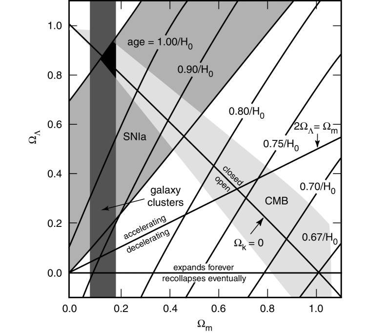
Figure 8.1: Observational constraints on two fundamental cosmological parameters. The area labeled galaxy clusters shows the constraints obtained in this work.

Chapter 9 Summary

An X-ray selected and X-ray flux-limited sample comprising the 63 X-ray brightest galaxy clusters in the sky (excluding the galactic band, called HIFLUGCS) has been constructed based on the ROSAT All-Sky Survey. The flux limit has been set at $2\,\times 10^{-11}\,{\rm ergs\,s^{-1}\,cm^{-2}}$ in the energy band $0.1-2.4\,{\rm keV}$. It has been shown that a high completeness is indicated by several tests. Due to the high flux limit this sample can be used for a variety of applications requiring a statistical cluster sample without any corrections to the effective survey volume.

Mainly high quality pointed observations have been used to determine fluxes and physical cluster parameters. It has been shown that a tight correlation exists between the X-ray luminosity and the gravitational mass using HIFLUGCS and an extended sample of 106 galaxy clusters. The relation and its scatter have been quantified using different fitting methods. A comparison to theoretical and numerical predictions shows an overall agreement. This relation may be directly applied in large X-ray cluster surveys or dark matter simulations for conversions between X-ray luminosity and gravitating mass.

Data from the performance verification phase of the recently launched X-ray satellite observatory XMM-Newton on the galaxy cluster Abell 1835 has been analyzed, in order to test the assumption of isothermality of the cluster gas in the outer parts applied throughout the work. It has been found that the measured outer temperature profile is consistent with being isothermal. In the inner regions a clear drop of the temperature by a factor of two has been found.

Physical properties of the cluster sample have been studied by analyzing relations between different cluster parameters. The overall properties are well understood but in detail deviations from simple expectations have been found. It has been found that the gas mass fraction does not vary as a function of intracluster gas temperature. For galaxy groups ($k_{\rm B}T_{\rm X}\lesssim 2$ keV), however, a steep drop of $f_{\rm gas}$ has been observed. No clear trend of a variation of the shape of the surface brightness profile, i.e. $\beta$, has been observed as a function of temperature. The $L_{\rm X}$–$T_{\rm X}$ relation has been found to be steeper than expected from simple self similar models, as has been found by previous authors. But no clear deviations from a power law shape down to $k_{\rm B}T_{\rm X}=0.7$ keV have been found. The $M_{\rm tot}$–$T_{\rm X}$ relation found here is steeper than expected from self similar models and its normalization is lower compared to hydrodynamic simulations, in agreement with previous findings. Suggested scenarios to account for these deviations, including heating and cooling processes, and observational difficulties have been described. It appears that a blend of different effects, possibly including a variation of mean formation redshift with system mass, is needed to account for the observations presented here.

Using HIFLUGCS the gravitational mass function has been determined for the mass interval $3.5\times 10^{13}<M_{200}<5.2\times 10^{15}\,h_{50}^{-1}\,M_{\odot}$. Comparison with Press–Schechter mass functions has yielded tight constraints on the mean matter density in the universe and the amplitude of density fluctuations. The large covered mass range has allowed to put constraints on the parameters individually. Specifically it has been found that $\Omega_{\rm m}=0.12^{+0.06}_{-0.04}$ and $\sigma_{8}=0.96^{+0.15}_{-0.12}$ (90 % c.l. statistical uncertainty). This result is consistent with two more estimates of $\Omega_{\rm m}$ obtained in this work using different methods. The mean intracluster gas fraction of the 106 clusters in the extended sample combined with predictions from the theory of nucleosynthesis indicates $\Omega_{\rm m}\lesssim 0.34$. The cluster mass to light ratio multiplied by the mean luminosity density implies $\Omega_{\rm m}\approx 0.15$. Various tests for systematic uncertainties have been performed, including comparison of the Press–Schechter mass function with the most recent results from large $N$-body simulations, yielding deviations smaller than the statistical uncertainties. For comparison the best fit $\Omega_{\rm m}$ values for fixed $\sigma_{8}$ values have been determined yielding the relation $\sigma_{8}=0.43\,\Omega_{\rm m}^{-0.38}$.

The mass function has been integrated to obtain the fraction of the total gravitating mass in the universe contained in galaxy clusters. Normalized to the critical density it has been found that $\Omega_{\rm Cluster}=0.012^{+0.003}_{-0.004}$ for cluster masses larger than $6.4^{+0.7}_{-0.6}\times 10^{13}\,h_{50}^{-1}\,M_{\odot}$. With the value for $\Omega_{\rm m}$ determined here this implies that about 90 % of the mass in the universe resides outside virialized cluster regions. Similarly it has been found that the fraction of the total gravitating mass which is contained in the intracluster gas, $\Omega_{\rm b,Cluster}=0.0015^{+0.0002}_{-0.0001}\,h_{50}^{-1.5}$ for gas masses larger than $6.9^{+1.4}_{-1.5}\times 10^{12}\,h_{50}^{-5/2}\,M_{\odot}$, is very small.

Appendix A Acknowledgements

During the preparation of this work I have benefitted from many people. Here I would like to express my gratitude to a few of them.

Hans Böhringer is an excellent scientist and I have gained a lot from discussions with him. He has supported this work in various ways by giving advice, encouraging independent initiatives, and providing the chance to participate in exciting related projects. Gregor Morfill has facilitated the start of this work and has been supporting it continuously. Joachim Trümper has made possible a valuable research visit to Tokyo Metropolitan University. My officemate Peter Schuecker has introduced me to a variety of interesting subjects by sharing his knowledge during innumerable discussions and his kind attitude has ensured a friendly relation in the tiny ‘container’ as well as in the spacious new building. With the members of the galaxy cluster group at MPE, especially Yasushi Ikebe, Paul Lynam, Alexis Finoguenov, and Jörg Retzlaff, I have enjoyed exciting scientific and worldly discussions. My wife Angelika has given me continuous encouragement especially during difficult stages.

ASCA temperatures for two clusters in this work have been determined while enjoying the outstanding hospitality of the cluster group at Tokyo Metropolitan University, especially Takaya Ohashi, Ken’ichi Kikuchi, Akihiro Kushino, Tae Furusho, and Yoshitaka Ishisaki. Useful discussions about the XMM-Newton background determination have been held with Sébastien Majerowicz, Doris Neumann, and Monique Arnaud at CEA-Saclay. The person who initially drew my attention to galaxy clusters was Simon White by advising a seminar talk at the University of Munich.

This work has benefitted a lot from the use of unpublished catalogs from the REFLEX and NORAS teams. Yasushi Ikebe has provided three cluster temperatures prior to publication. Volker Mueller, Jörg Retzlaff and Peter Schuecker have provided results from OCDM simulations. Marisa Girardi provided electronic tables of the mass determinations based on galaxy velocity dispersions. Alexis Finoguenov provided electronic tables of partly unpublished X-ray mass measurements. Robert Schmidt has made available electronic tables of the Chandra results on A1835. Some of the basic programs used in this work are extensions of software developped by former cluster group members, especially Raimund Schwarz. The code for calculation of the universal mass function has been provided by Adrian Jenkins. The code for calculation of the Eisenstein and Hu, transfer function has been provided by these authors. Software provided by Manami Sasaki has been used to correct individual photons, detected by XMM-Newton, for vignetting, and arf files have been obtained from Kyoko Matsushita. The BCES regression software has been provided by Michael Akritas, Tina Bird, and Matthew Bershady. A style file for the deluxetable environment based on the AASTEX document class has been obtained from Alexey Vikhlinin. Figure 8.1 has been prepared based on Figures presented in de Bernardis et al., and Bahcall et al., with the help of Barbara Mory.

The author acknowledges the dedicated work of and the benefit from discussions with the ROSAT and XMM-Newton hardware, software, and calibration teams at MPE. Extensive use has been made of the ROSAT Data Archive at MPE, of the NASA/IPAC Extragalactic Database (NED) which is operated by the Jet Propulsion Laboratory, Caltech, under contract with the National Aeronautics and Space Administration, and of observations obtained with XMM-Newton  an ESA science mission with instruments and contributions directly funded by ESA Member States and the USA (NASA).

References

- Abell, (1958) Abell, G. O. (1958). The distribution of rich clusters of galaxies. ApJS, 3:211–288.
- Abell et al., (1989) Abell, G. O., Corwin Jr., H. G., and Olowin, R. P. (1989). A catalog of rich clusters of galaxies. ApJS, 70:1–138.
- Akritas and Bershady, (1996) Akritas, M. G. and Bershady, M. A. (1996). Linear regression for astronomical data with measurement errors and intrinsic scatter. ApJ, 470:706–714. http://www.astro.wisc.edu/mab/archive/stats.html.
- Alcock et al., (1997) Alcock, C., Allsman, R. A., Alves, D., Axelrod, T. S., Becker, A. C., Bennett, D. P., Cook, K. H., Freeman, K. C., Griest, K., Guern, J., Lehner, M. J., Marshall, S. L., Peterson, B. A., Pratt, M. R., Quinn, P. J., Rodgers, A. W., Stubbs, C. W., Sutherland, W., and Welch, D. L. (1997). The MACHO project Large Magellanic Cloud microlensing results from the first two years and the nature of the galactic dark halo. ApJ, 486:697–726.
- Alcock et al., (2000) Alcock, C., Allsman, R. A., Alves, D. R., Axelrod, T. S., Becker, A. C., Bennett, D. P., Cook, K. H., Dalal, N., Drake, A. J., Freeman, K. C., Geha, M., Griest, K., Lehner, M. J., Marshall, S. L., Minniti, D., Nelson, C. A., Peterson, B. A., Popowski, P., Pratt, M. R., Quinn, P. J., Stubbs, C. W., Sutherland, W., Tomaney, A. B., Vandehei, T., and Welch, D. L. (2000). The MACHO project: Microlensing results from 5.7 years of Large Magellanic Cloud observations. ApJ, 542:281–307.
- Allen, (1998) Allen, S. W. (1998). Resolving the discrepancy between X-ray and gravitational lensing mass measurements for clusters of galaxies. MNRAS, 296:392–406.
- Allen et al., (1992) Allen, S. W., Edge, A. C., Fabian, A. C., Böhringer, H., Crawford, C. S., Ebeling, H., Johnstone, R. M., Naylor, T., and Schwarz, R. A. (1992). Optical spectroscopy of the ROSAT X-ray brightest clusters. MNRAS, 259:67–81.
- Allen and Fabian, (1998) Allen, S. W. and Fabian, A. C. (1998). The impact of cooling flows on the – relation for the most luminous clusters. MNRAS, 297:L57–L62.
- Allen et al., (1996) Allen, S. W., Fabian, A. C., Edge, A. C., Bautz, M. W., Furuzawa, A., and Tawara, Y. (1996). ASCA and ROSAT observations of distant, massive cooling flows. MNRAS, 283:263–281.
- Anders and Grevesse, (1989) Anders, E. and Grevesse, N. (1989). Abundances of the elements - meteoritic and solar. Geochim. Cosmochim. Acta, 53:197–214.
- Andersen and Owen, (1994) Andersen, V. and Owen, F. N. (1994). A comparison of the richness of clusters and groups of galaxies. AJ, 108:361–367.
- Arnaud, (1996) Arnaud, K. A. (1996). XSPEC: The first ten years. In ASP Conf. Ser. 101: Astronomical Data Analysis Software and Systems V, volume 5, pages 17–20.
- Arnaud and Evrard, (1999) Arnaud, M. and Evrard, A. E. (1999). The – relation and intracluster gas fractions of X-ray clusters. MNRAS, 305:631–640.
- Arnaud et al., (1996) Arnaud, M., Rothenflug, R., Böhringer, H., Neumann, D., and Yamashita, K. (1996). ROSAT/Ginga observation of the galaxy cluster A3921. In Yamashita, K. and Watanabe, T., editors, UV and X-ray Spectroscopy of Astrophysical and Laboratory Plasmas, page 163, Tokyo, Japan. Universal Academy Press.
- Arnaud et al., (1992) Arnaud, M., Rothenflug, R., Boulade, O., Vigroux, L., and Vangioni-Flam, E. (1992). Some constraints on the origin of the iron enriched intracluster medium. A&A, 254:49–64.
- Avni and Bahcall, (1980) Avni, Y. and Bahcall, J. N. (1980). On the simultaneous analysis of several complete samples – the and variables, with applications to quasars. ApJ, 235:694–716.
- Bahcall and Cen, (1992) Bahcall, N. A. and Cen, R. (1992). Galaxy clusters and Cold Dark Matter – a low-density unbiased universe? ApJ, 398:L81–L84.
- Bahcall and Cen, (1993) Bahcall, N. A. and Cen, R. (1993). The mass function of clusters of galaxies. ApJ, 407:L49–L52.
- Bahcall et al., (1995) Bahcall, N. A., Lubin, L. M., and Dorman, V. (1995). Where is the dark matter? ApJ, 447:L81–L85.
- Bahcall et al., (1999) Bahcall, N. A., Ostriker, J. P., Perlmutter, S., and Steinhardt, P. J. (1999). The cosmic triangle: Revealing the state of the universe. Sci, 284:1481–1488.
- Balbi et al., (2000) Balbi, A., Ade, P., Bock, J., Borrill, J., Boscaleri, A., de Bernardis, P., Ferreira, P. G., Hanany, S., Hristov, V., Jaffe, A. H., Lee, A. T., Oh, S., Pascale, E., Rabii, B., Richards, P. L., Smoot, G. F., Stompor, R., Winant, C. D., and Wu, J. H. P. (2000). Constraints on cosmological parameters from MAXIMA-1. ApJ, 545:L1–L4.
- Balogh et al., (2001) Balogh, M. L., Pearce, F. R., Bower, R. G., and Kay, S. T. (2001). Revisiting the cosmic cooling crisis. MNRAS, submitted. Preprint: astro-ph/0104041.
- Bardeen et al., (1986) Bardeen, J. M., Bond, J. R., Kaiser, N., and Szalay, A. S. (1986). The statistics of peaks of Gaussian random fields. ApJ, 304:15–61.
- Beers et al., (1991) Beers, T. C., Gebhardt, K., Forman, W., Huchra, J. P., and Jones, C. (1991). A dynamical analysis of twelve clusters of galaxies. AJ, 102:1581–1609.
- Berghöfer et al., (1999) Berghöfer, T. W., Bowyer, S., and Korpela, E. (1999). EUVE observations of clusters of galaxies: M87. In Böhringer, H., Feretti, L., and Schuecker, P., editors, Diffuse Thermal and Relativistic Plasma in Galaxy Clusters, pages 207–211, Garching, Germany. MPE Report 271.
- Beuing et al., (1999) Beuing, J., Döbereiner, S., Böhringer, H., and Bender, R. (1999). X-ray luminosities for a magnitude-limited sample of early-type galaxies from the ROSAT All-Sky Survey. MNRAS, 302:209–221.
- Binggeli et al., (1988) Binggeli, B., Sandage, A., and Tammann, G. A. (1988). The luminosity function of galaxies. ARA&A, 26:509–560.
- Biviano et al., (1993) Biviano, A., Girardi, M., Giuricin, G., Mardirossian, F., and Mezzetti, M. (1993). The mass function of nearby galaxy clusters. ApJ, 411:L13–L16.
- Böhringer, (1993) Böhringer, H. (1993). ROSAT observations of galaxy clusters and cosmological implications. Adv. Space Res., 13:181–190.
- Böhringer, (1995) Böhringer, H. (1995). Clusters of galaxies. In Böhringer, H., Trümper, J., and Morfill, G. E., editors, Texas Symposium on Relativistic Astrophysics and Cosmology, Annals of the New York Academy of Science, volume 759, pages 67–86.
- (31) Böhringer, H., Collins, C. A., Guzzo, L., Schuecker, P., Voges, W., Neumann, D. M., Schindler, S., Chincarini, G., De Grandi, S., Cruddace, R. G., Edge, A. C., Reiprich, T. H., and Shaver, P. (2001a). The REFLEX galaxy cluster survey IV: The X-ray luminosity function. A&A, submitted. Preprint: astro-ph/0106243.
- Böhringer and Hensler, (1989) Böhringer, H. and Hensler, G. (1989). Metallicity-dependence of radiative cooling in optically thin, hot plasmas. A&A, 215:147–149.
- (33) Böhringer, H., Schuecker, P., Guzzo, L., Collins, C. A., Voges, W., Schindler, S., Neumann, D. M., Cruddace, R. G., De Grandi, S., Chincarini, G., Edge, A. C., MacGillivray, H. T., and Shaver, P. (2001b). The ROSAT-ESO flux limited X-ray (REFLEX) galaxy cluster survey. I. The construction of the cluster sample. A&A, 369:826–850.
- Böhringer et al., (2000) Böhringer, H., Voges, W., Huchra, J. P., McLean, B., Giacconi, R., Rosati, P., Burg, R., Mader, J., Schuecker, P., Simiç, D., Komossa, S., Reiprich, T. H., Retzlaff, J., and Trümper, J. (2000). The Northern ROSAT All-Sky (NORAS) galaxy cluster survey. I. X-ray properties of clusters detected as extended X-ray sources. ApJS, 129:435–474.
- Bolte and Hogan, (1995) Bolte, M. and Hogan, C. J. (1995). Conflict over the age of the universe. Nat, 376:399.
- Bond et al., (1991) Bond, J. R., Cole, S., Efstathiou, G., and Kaiser, N. (1991). Excursion set mass functions for hierarchical Gaussian fluctuations. ApJ, 379:440–460.
- Borgani and Guzzo, (2001) Borgani, S. and Guzzo, L. (2001). X-ray clusters of galaxies as tracers of structure in the universe. Nat, 409:39–45.
- Borgani et al., (1999) Borgani, S., Rosati, P., Tozzi, P., and Norman, C. (1999). Cosmological constraints from the ROSAT Deep Cluster Survey. ApJ, 517:40–53.
- Bower, (1991) Bower, R. G. (1991). The evolution of groups of galaxies in the Press-Schechter formalism. MNRAS, 248:332–352.
- Bower et al., (2001) Bower, R. G., Benson, A. J., Lacey, C. G., Baugh, C. M., Cole, S., and Frenk, C. (2001). The impact of galaxy formation on the X-ray evolution of clusters. MNRAS, accepted. Preprint: astro-ph/0006109.
- Bowyer et al., (1999) Bowyer, S., Berghöfer, T. W., and Korpela, E. (1999). A reanalysis of EUV emission in clusters of galaxies. In Böhringer, H., Feretti, L., and Schuecker, P., editors, Diffuse Thermal and Relativistic Plasma in Galaxy Clusters, pages 201–206, Garching, Germany. MPE Report 271.
- Briel et al., (1992) Briel, U. G., Henry, J. P., and Böhringer, H. (1992). Observation of the Coma cluster of galaxies with ROSAT during the All-Sky Survey. A&A, 259:L31.
- Brighenti and Mathews, (2001) Brighenti, F. and Mathews, W. G. (2001). Entropy evolution in galaxy groups and clusters: a comparison of external and internal heating. ApJ, 553:103–120.
- Bronstein and Semendjajew, (1980) Bronstein, I. N. and Semendjajew, K. A. (1980). Taschenbuch der Mathematik. Verlag Harri Deutsch, Thun und Frankfurt/Main, 19. edition.
- Bryan, (2000) Bryan, G. L. (2000). Explaining the entropy excess in clusters and groups of galaxies without additional heating. ApJ, 544:L1–L5.
- Burkert, (1995) Burkert, A. (1995). The structure of dark matter halos in dwarf galaxies. ApJ, 447:L25–L28.
- Burles and Tytler, (1998) Burles, S. and Tytler, D. (1998). The Deuterium abundance toward Q1937–1009. ApJ, 499:699–712.
- Capelato et al., (1991) Capelato, H. V., Mazure, A., Proust, D., Vanderriest, C., Lemonnier, J. P., and Sodre, L. (1991). New measurements of radial velocities in clusters of galaxies. III. A&AS, 90:355–364.
- Carlberg et al., (1997) Carlberg, R. G., Morris, S. L., Yee, H. K. C., and Ellingson, E. (1997). Redshift evolution of galaxy cluster densities. ApJ, 479:L19–L22.
- Carlstrom et al., (1996) Carlstrom, J. E., Joy, M., and Grego, L. (1996). Interferometric imaging of the Sunyaev-Zeldovich effect at 30 GHz. ApJ, 456:L75–L78.
- Carretta et al., (2000) Carretta, E., Gratton, R. G., Clementini, G., and Fusi Pecci, F. (2000). Distances, ages, and epoch of formation of globular clusters. ApJ, 533:215–235.
- Carroll et al., (1992) Carroll, S. M., Press, W. H., and Turner, E. L. (1992). The cosmological constant. ARA&A, 30:499–542.
- Cavaliere and Fusco-Femiano, (1976) Cavaliere, A. and Fusco-Femiano, R. (1976). X-rays from hot plasma in clusters of galaxies. A&A, 49:137–144.
- Cayatte et al., (1990) Cayatte, V., van Gorkom, J. H., Balkowski, C., and Kotanyi, C. (1990). VLA observations of neutral hydrogen in Virgo cluster galaxies. I - the atlas. AJ, 100:604–634.
- Cirimele et al., (1997) Cirimele, G., Nesci, R., and Trevese, D. (1997). An X-ray and optical study of matter distribution in clusters of galaxies. ApJ, 475:11–19.
- Clarke et al., (2001) Clarke, T. E., Kronberg, P. P., and Böhringer, H. (2001). A new radio-X-ray probe of galaxy cluster magnetic fields. ApJ, 547:L111–L114.
- Colberg et al., (1999) Colberg, J. M., White, S. D. M., Jenkins, A., and Pearce, F. R. (1999). Linking cluster formation to large-scale structure. MNRAS, 308:593–598.
- Colless and Hewett, (1987) Colless, M. and Hewett, P. (1987). The dynamics of rich clusters. I - velocity data. MNRAS, 224:453–472.
- da Costa et al., (1998) da Costa, L. N., Willmer, C. N. A., Pellegrini, P. S., Chaves, O. L., Rité, C., Maia, M. A. G., Geller, M. J., Latham, D. W., Kurtz, M. J., Huchra, J. P., Ramella, M., Fairall, A. P., Smith, C., and Lípari, S. (1998). The southern sky redshift survey. AJ, 116:1–7.
- David, (1997) David, L. P. (1997). The baryonic content of galaxies and clusters. ApJ, 484:L11–L15.
- David et al., (1990) David, L. P., Arnaud, K. A., Forman, W., and Jones, C. (1990). Einstein observations of the Hydra A cluster and the efficiency of galaxy formation in groups and clusters. ApJ, 356:32–40.
- David et al., (1995) David, L. P., Jones, C., and Forman, W. (1995). Cosmological implications of ROSAT observations of groups and clusters of galaxies. ApJ, 445:578–590.
- David et al., (1993) David, L. P., Slyz, A., Jones, C., Forman, W., and Vrtilek, S. D. (1993). A catalog of intracluster gas temperatures. ApJ, 412:479–488.
- Davis et al., (1995) Davis, D. S., Bird, C. M., Mushotzky, R. F., and Odewahn, S. C. (1995). Abell 548: an X-ray and optical analysis of substructure. ApJ, 440:48–59.
- Davis et al., (1999) Davis, D. S., Mulchaey, J. S., and Mushotzky, R. F. (1999). The enrichment history of hot gas in poor galaxy groups. ApJ, 511:34–40.
- Davoust and Considere, (1995) Davoust, E. and Considere, S. (1995). Kinematical observations of pairs of galaxies. A&AS, 110:19–26.
- de Bernardis et al., (2001) de Bernardis, P., Ade, P. A. R., Bock, J. J., Bond, J. R., Borrill, J., Boscaleri, A., Coble, K., Contaldi, C. R., Crill, B. P., De Troia, G., Farese, P., Ganga, K., Giacometti, M., Hivon, E., Hristov, V. V., Iacoangeli, A., Jaffe, A. H., Jones, W. C., Lange, A. E., Martinis, L., Masi, S., Mason, P., Mauskopf, P. D., Melchiorri, A., Montroy, T., Netterfield, C. B., Pascale, E., Piacentini, F., Pogosyan, D., Polenta, G., Pongetti, F., Prunet, S., Romeo, G., Ruhl, J. E., and Scaramuzzi, F. (2001). Multiple peaks in the angular power spectrum of the cosmic microwave background: Significance and consequences for cosmology. ApJ, submitted. Preprint: astro-ph/0105296.
- de Bernardis et al., (2000) de Bernardis, P., Ade, P. A. R., Bock, J. J., Bond, J. R., Borrill, J., Boscaleri, A., Coble, K., Crill, B. P., De Gasperis, G., Farese, P. C., Ferreira, P. G., Ganga, K., Giacometti, M., Hivon, E., Hristov, V. V., Iacoangeli, A., Jaffe, A. H., Lange, A. E., Martinis, L., Masi, S., Mason, P. V., Mauskopf, P. D., Melchiorri, A., Miglio, L., Montroy, T., Netterfield, C. B., Pascale, E., Piacentini, F., Pogosyan, D., Prunet, S., Rao, S., Romeo, G., Ruhl, J. E., Scaramuzzi, F., Sforna, D., and Vittorio, N. (2000). A flat universe from high-resolution maps of the cosmic microwave background radiation. Nat, 404:955–959.
- De Grandi et al., (1999) De Grandi, S., Böhringer, H., Guzzo, L., Molendi, S., Chincarini, G., Collins, C., Cruddace, R., Neumann, D., Schindler, S., Schuecker, P., and Voges, W. (1999). A flux-limited sample of bright clusters of galaxies from the southern part of the ROSAT All-Sky Survey: The catalog and –. ApJ, 514:148–163.
- de Vaucouleurs et al., (1991) de Vaucouleurs, G., de Vaucouleurs, A., Corwin, J. R., Buta, R. J., Paturel, G., and Fouque, P. (1991). Third Reference Catalogue of Bright Galaxies (RC3). Springer Verlag, New York, USA.
- dell’Antonio et al., (1994) dell’Antonio, I. P., Geller, M. J., and Fabricant, D. G. (1994). X-ray and optical properties of groups of galaxies. AJ, 107:427–447.
- den Hartog and Katgert, (1996) den Hartog, R. and Katgert, P. (1996). On the dynamics of the cores of galaxy clusters. MNRAS, 279:349–388.
- Dickey and Lockman, (1990) Dickey, J. M. and Lockman, F. J. (1990). HI in the galaxy. ARA&A, 28:215–61. http://imagelib.ncsa.uiuc.edu/project/document/95.FL.01.
- Dolag and Schindler, (2000) Dolag, K. and Schindler, S. (2000). The effect of magnetic fields on the mass determination of clusters of galaxies. A&A, 364:491–496.
- Dressler, (1984) Dressler, A. (1984). The evolution of galaxies in clusters. ARA&A, 22:185–222.
- Dressler and Shectman, (1988) Dressler, A. and Shectman, S. A. (1988). Evidence for substructure in rich clusters of galaxies from radial-velocity measurements. AJ, 95:985–995.
- Ebeling et al., (1998) Ebeling, H., Edge, A. C., Böhringer, H., Allen, S. W., Crawford, C. S., Fabian, A. C., Voges, W., and Huchra, J. P. (1998). The ROSAT Brightest Cluster Sample – I. The compilation of the sample and the cluster log –log distribution. MNRAS, 301:881–914.
- Ebeling et al., (1997) Ebeling, H., Edge, A. C., Fabian, A. C., Allen, S. W., Crawford, C. S., and Böhringer, H. (1997). The ROSAT brightest cluster sample (BCS): The cluster X-ray luminosity function within . ApJ, 479:L101–L104.
- Ebeling et al., (1996) Ebeling, H., Voges, W., Böhringer, H., Edge, A. C., Huchra, J. P., and Briel, U. G. (1996). Properties of the X-Ray-Brightest Abell-Type Clusters of Galaxies (XBACs) from ROSAT All-Sky Survey data. MNRAS, 281:799–829.
- (80) Edge, A. C. and Stewart, G. C. (1991a). EXOSAT observations of clusters of galaxies – I. the X-ray data. MNRAS, 252:414–427.
- (81) Edge, A. C. and Stewart, G. C. (1991b). EXOSAT observations of clusters of galaxies – II. X-ray to optical correlations. MNRAS, 252:428–441.
- Edge et al., (1990) Edge, A. C., Stewart, G. C., Fabian, A. C., and Arnaud, K. A. (1990). An X-ray flux-limited sample of clusters of galaxies. MNRAS, 245:559–569.
- Efstathiou et al., (1988) Efstathiou, G., Frenk, C. S., White, S. D. M., and Davis, M. (1988). Gravitational clustering from scale-free initial conditions. MNRAS, 235:715–748.
- Eisenstein and Hu, (1998) Eisenstein, D. J. and Hu, W. (1998). Baryonic features in the matter transfer function. ApJ, 496:605–614.
- Eke et al., (1996) Eke, V. R., Cole, S., and Frenk, C. S. (1996). Cluster evolution as a diagnostic for Omega. MNRAS, 282:263–280.
- Elbaz et al., (1995) Elbaz, D., Arnaud, M., and Böhringer, H. (1995). The gas distribution and binding mass in the A2163 cluster. A&A, 293:337–346.
- Ettori and Fabian, (1999) Ettori, S. and Fabian, A. C. (1999). ROSAT PSPC observations of 36 high-luminosity clusters of galaxies: constraints on the gas fraction. MNRAS, 305:834–848.
- Ettori and Fabian, (2000) Ettori, S. and Fabian, A. C. (2000). Relations with the gravitating mass in X-ray galaxy clusters. In Plionis, M. and Georgantopoulos, I., editors, Large Scale Structure in the X-ray Universe, pages 355–356, Paris, France. Atlantisciences.
- Evrard, (1997) Evrard, A. E. (1997). The intracluster gas fraction in X-ray clusters - constraints on the clustered mass density. MNRAS, 292:289–297.
- Evrard and Henry, (1991) Evrard, A. E. and Henry, J. P. (1991). Expectations for X-ray cluster observations by the ROSAT satellite. ApJ, 383:95–103.
- Evrard et al., (1996) Evrard, A. E., Metzler, C. A., and Navarro, J. F. (1996). Mass estimates of X-ray clusters. ApJ, 469:494–507.
- Fabian, (1994) Fabian, A. C. (1994). Cooling flows in clusters of galaxies. ARA&A, 32:277–318.
- Fabian et al., (1981) Fabian, A. C., Hu, E. M., Cowie, L. L., and Grindlay, J. (1981). The distribution and morphology of X-ray–emitting gas in the core of the Perseus cluster. ApJ, 248:47–54.
- Felten, (1976) Felten, J. E. (1976). On Schmidt’s estimator and other estimators of luminosity functions. ApJ, 207:700–709.
- Fields et al., (1997) Fields, B. D., Mathews, G. J., and Schramm, D. N. (1997). Halo white dwarfs and the hot intergalactic medium. ApJ, 483:625–637.
- Finoguenov et al., (2001) Finoguenov, A., Reiprich, T. H., and Böhringer, H. (2001). Details of the mass-temperature relation for clusters of galaxies. A&A, 368:749–759.
- Fox and Loeb, (1997) Fox, D. C. and Loeb, A. (1997). Do the electrons and ions in X-ray clusters share the same temperature? ApJ, 491:459–466.
- Frenk et al., (1999) Frenk, C. S., White, S. D. M., Bode, P., Bond, J. R., Bryan, G. L., Cen, R., Couchman, H. M. P., Evrard, A. E., Gnedin, N., Jenkins, A., Khokhlov, A. M., Klypin, A., Navarro, J. F., Norman, M. L., Ostriker, J. P., Owen, J. M., Pearce, F. R., Pen, U. ., Steinmetz, M., Thomas, P. A., Villumsen, J. V., Wadsley, J. W., Warren, M. S., Xu, G., and Yepes, G. (1999). The Santa Barbara cluster comparison project: A comparison of cosmological hydrodynamics solutions. ApJ, 525:554–582.
- Fukazawa, (1997) Fukazawa, Y. (1997). X-Ray Study of Metal Enrichment Processes of Hot Gas in Clusters of Galaxies. PhD thesis, Univ. Tokyo.
- Fukazawa et al., (1998) Fukazawa, Y., Makishima, K., Tamura, T., Ezawa, H., Xu, H., Ikebe, Y., Kikuchi, K., and Ohashi, T. (1998). ASCA measurements of silicon and iron abundances in the intracluster medium. PASJ, 50:187–193.
- Fukuda et al., (1998) Fukuda, Y., Hayakawa, T., Ichihara, E., Inoue, K., Ishihara, K., Ishino, H., Itow, Y., Kajita, T., Kameda, J., Kasuga, S., Kobayashi, K., Kobayashi, Y., Koshio, Y., Miura, M., Nakahata, M., and et al. (1998). Evidence for oscillation of atmospheric neutrinos. Phys. Rev. Lett., 81:1562–1567.
- Fukugita et al., (1998) Fukugita, M., Hogan, C. J., and Peebles, P. J. E. (1998). The cosmic baryon budget. ApJ, 503:518–530.
- Fusco-Femiano, (1999) Fusco-Femiano, R. (1999). Hard X-ray emission in clusters of galaxies. In Böhringer, H., Feretti, L., and Schuecker, P., editors, Diffuse Thermal and Relativistic Plasma in Galaxy Clusters, pages 191–196, Garching, Germany. MPE Report 271.
- Garcia, (1995) Garcia, A. M. (1995). Compact groups of galaxies in the nearby universe. A&A, 297:56–60.
- (105) Girardi, M., Borgani, S., Giuricin, G., Mardirossian, F., and Mezzetti, M. (1998a). The observational mass function of nearby galaxy clusters. ApJ, 506:45–52.
- Girardi et al., (2000) Girardi, M., Borgani, S., Giuricin, G., Mardirossian, F., and Mezzetti, M. (2000). Optical luminosities and mass-to-light ratios of nearby galaxy clusters. ApJ, 530:62–79.