Investigating lensing by absorbers in the 2dF-Quasar survey

We use the first data release of the 2-degree Field Quasar survey to investigate the effect of gravitational magnification by foreground absorbing systems on background quasars. We select two populations of quasars from this sample: one with strong Mg ii/Fe ii absorbers and one without. The selection is done in such a way that the two populations have the same redshift distribution and the absorber detection procedure discards possible biases with quasar magnitude. We then compare their magnitude distributions and find a relative excess of bright quasars with absorbers. This effect is detected at the 2.4, 3.7 and 4.4$\sigma$ levels in u-, b- and r-bands. Various explanations of the observed phenomenon are considered and several lines of evidence point towards gravitational lensing causing some of the differences observed in the magnitude distributions. We note that physical quasar-absorber associations may contribute to some extent to the observed correlations for low quasar-absorber velocity differences. We discuss the implications of these findings and propose future work which will allow us to strengthen and extend the results presented here.

1 Introduction

Luminous quasi-stellar objects, hereafter quasars, permit the detection of arbitrarily faint galactic systems through absorption in their spectra. These absorbers are believed to trace various types of systems (disks, dwarfs, low surface brightness galaxies) and/or different regions of galaxies (the innermost part, outflows). Detecting such a system in the spectrum of a quasar indicates the presence of a matter overdensity along its line-of-sight and such a concentration of matter may well act as a lens on the background quasar. This scenario is then expected to affect the magnitude distribution of a quasar population showing absorption systems (Bartelmann & Loeb 1995, Pei 1995, Perna et al. 1997, Smette et al. 1997).
If some absorbers, for example with high H i column densities, trace distant galaxies, the associated lensing effects, for impact parameters greater than $\sim 10$ kpc, will likely modify the flux of the source without producing new additional images. Since the intrinsic luminosity of a given quasar is not known a-priori, such an effect cannot be detected for an individual object but requires a statistical analysis performed with a large homogeneous sample.

For a magnitude limited sample of quasars, two effects of gravitational magnification come into play: the flux received from distant sources is boosted, increasing the probability of observing quasars behind absorbers, while the solid angle behind absorbers is gravitationally enlarged, which then lowers the density of background quasars. The net result of these competing effects (an increase or decrease of the number counts of quasars with an absorber) depends on whether the loss of sources due to dilution is balanced by the gain of sources due to flux magnification (Narayan 1989). Sources with flat luminosity functions, like faint quasars, are depleted by magnification while the number density of sources with steep luminosity functions, like bright quasars, is increased. This effect is called the magnification bias (e.g. Schneider et al. 1992).

Attempts to quantify this phenomenon have been made in the past through both theoretical modeling and direct observations. Pei (1995) estimated the effects of gravitational lensing by cosmologically distributed dark matter halos on the quasar luminosity function; Bartelmann & Loeb (1995) and Smette et al. (1997) showed how the statistics of Damped Ly-$\alpha$ systems are affected by lensing; Perna et al. (1997) estimated that for bright quasars changes in magnitudes due to gravitational lensing by spiral galaxies are stronger than obscuration effects which give rise to the opposite trend. More recently, Maller et al. (2002) have shown that the Sloan Digital Sky Survey (SDSS; York et al. 2000) combined with future space-based missions (such as the Galaxy Evolution Explorer satellite; Milliard et al. 2001) will provide the necessary data to constrain the mass to gas ratio of certain types of absorbers by using the gravitational lensing effects they produce on background quasars.

On the observational side, one approach consists of fitting lensing models to the redshift evolution of quasar absorbers to disentangle intrinsic evolution from gravitational lensing (Thomas & Webster 1990; Steidel & Sargent 1992, Borgeest & Mehlert 1993). All these studies found the effect of lensing to be small for the range of redshifts and equivalent widths they used. Another approach first suggested by York et al. (1991) is to divide quasar spectra into a bright and a faint sample in order to determine the incidence of absorbers in each sample separately. In their study, York et al. found no evidence for gravitational lensing, except perhaps towards higher redshifts (z$\sim$3). Vanden Berk et al. (1996) extended the analysis to a larger sample of quasar spectra compiled from the literature. They found an excess of C iv absorbers in luminous quasars, as would be expected from a gravitational lensing effect, but did not find a similar trend in the available Mg ii sample. Recently, Le Brun et al. (2000) used a sample of 7 Damped Ly-$\alpha$ systems for which they identified the absorbing galaxies, measured the impact parameters, and derived the upper limit of 0.3 magnitude for the amplification factor.

Apart from the latter one, all these above mentioned studies used relatively weak absorber samples: considering Mg ii, most of the corresponding systems they used have an equivalent width ($0.2\lesssim\,$W${}_{0}\,(2796\,$Å$)\lesssim 1$ Å). As a result, the authors looked for the cumulative - and likely weak - lensing effects due to multiple absorbing systems along the line-of-sight of quasars. Here we adopt another strategy for unveiling the effects of gravitational lensing by absorbers: we focus on the strongest systems and look for their magnification bias. Indeed, despite the fact that such systems are rarer, some of them may actually probe the inner part of galactic halos and might therefore favor observable lensing effects. Being able to measure the associated magnification bias might be of great interest since it allows us to probe the dark matter distribution of distant baryonic systems seen in absorption. For a given distribution of impact parameters and for a given dark matter profile, an accurate measurement can then lead to some constrains on the average mass of these absorber systems.

In order to detect this effect, we use here the first release of the 2dF quasar survey (2QZ), i.e. a large and homogeneous sample of quasar spectra, to compare the magnitude distribution of quasars with a strong Mg ii absorber ($1.3\lesssim\,$W${}_{0}\,(2796+2803\,$Å$)\lesssim 9.0$ Å) to that of a reference population of quasars for which no such absorption was found.

This paper is organized as follows: in Sect. 2 we present the data and detail how we selected two unbiased samples of quasars, with and without absorbers. We then compare their magnitude distribution in Sect. 3 and find a significant difference between them. In Sect. 4 we review the effects expected from the presence of a system along a quasar line-of-sight and find gravitational lensing and physical associations to be the most likely explanations for the trend we observe. Finally, we discuss the implications of the results obtained and propose further extensions of this work to the larger sets of data which will become available soon.

2 The Data

Until recently only a few hundred quasar spectra were available for the detection of quasar absorbers. With the help of multi-fiber spectroscopy, surveys of thousands of quasars have become publicly available. A pioneer experiment in this area, the 2 degree field quasar redshift survey (2QZ) has already acquired more than $20,000$ quasar spectra (Boyle et al. 2001; Croom et al. 2001a; Hoyle et al. 2002) and provides an unprecedented source for statistical studies of quasars in a homogeneous sample.

2.1 The 2dF QSO Redshift Survey and associated quasar absorbers

The first data release of the 2QZ contains over ten thousand low resolution quasar spectra, taken with the 2-degree Field instrument at the Anglo-Australian Telescope in the range 3700 - 7500 Å. Quasar candidates with $18.25<b_{J}<20.85$ were selected from a single homogeneous color-based catalogue from APM (Automatic Plate Measuring) measurements of UK Schmidt photographic material. Note that the corresponding u- and r-band quasar catalogues are therefore not complete.
In our study we will use the absorber catalogue compiled by Outram et al. (2001). They examined visually the highest signal-to-noise ratio spectra in order to identify heavy element absorbers (hereafter, “metal” absorbers). Their aim was to compile a list of Damped Lyman $\alpha$ (DLA) candidates for further investigation. Starting from the 10k catalogue, the sub-sample used to optimize this “metal” search is defined according to the following criteria:

1. the sample is limited to quasars with $z_{\rm em}>0.5$;

2. only spectra with signal-to-noise ratio (S/N) greater than 15 in the range 4000-5000Å were selected. This S/N estimate is based on spectral variances measured from the 200 fibers in each APM field;

3. quasars exhibiting broad absorption lines or high ionization systems with $z_{\rm abs}\sim z_{\rm em}$ are excluded from the analysis.

This selection reduces the 10k release to a sample of 1264 quasars which were visually inspected for the detection of absorption lines. In order to avoid false detections, they require the presence of at least two absorber species at the same redshift. We refer the reader to Outram et al. (2001) for the details of the absorption line detection technique.

In this subsample of quasars, 129 spectra contain at least one absorption system and there remain 1135 quasars for which no absorption line was detected. In order to compare the magnitude distribution of these two samples, the corresponding quasars must be selected in a way that does not introduce any magnitude bias. The rest of the section describes the details of this selection.

2.1.1 The Absorber Population

In order to optimize the detection of statistical lensing effects, a large sample of strong absorbers is required. In the 2QZ the most commonly detected absorbers are Mg ii/Fe ii systems. Indeed, Mg ii absorption is a doublet, allowing for robust identification, and Fe ii lines present a variety of rest wavelengths and oscillator strengths, which eases Fe ii identification in a given wavelength range. The Mg ii/Fe ii absorbers identified by Outram et al. (2001) are strong systems with rest equivalent width of the Mg ii doublets ranging from 1.3 to 9.0 Å (see Table 4). In the following, all equivalent widths will refer to the one of the Mg ii doublet, as given by Outram et al. (2001). This preselection reduces the sample introduced above down to 109 quasars. The corresponding list is given in Appendix A. For our analysis, we do not take into account the small number of quasars which are not detected in the r-band: one quasar with an absorber (flagged R1 in Table 4) and 2% of the reference quasars, in order to analyze well-defined samples in every magnitude band. Lastly, since our goal is to look for gravitational lensing effects, we also exclude one system (flagged R2 in the Table) for which the absorber escape velocity is smaller than $3\,000$ km/s which indicates that the absorber is very likely physically associated to the quasar. In the six cases where two absorbers are detected in a single quasar spectrum (A flags), we consider only the one having the largest equivalent width. (Note that, given the small number of quasars concerned, using other choices do not significantly affect the results of this study). The resulting set of quasars with absorbers contains 108 objects and the reference population 1114. The selection steps are summarized in Table 3.

As mentioned in the introduction, the amplitude of gravitational lensing effects by absorbers is expected to be highest when absorbing systems probe the inner part of galactic halos. Such a situation is likely to occur when quasar spectra show strong Mg ii lines or a Damped Lyman-$\alpha$ absorber at z$\gtrsim$0.5 (Steidel 1995, Le Brun et al. 2000). Several theoretical studies have investigated the corresponding lensing effects (Pei 1995, Bartelmann & Loeb 1995, Perna et al. 1997, Smette et al. 1997). In the present study, it is important to note that our absorber sample is actually expected to present such properties: strong Mg ii/Fe ii systems have proven to be excellent tracers of DLAs. Indeed, although a number of DLAs are known at high-redshifts (Storrie-Lombardi et al. 1996; Storrie-Lombardi & Wolfe 2000; Péroux et al. 2001) due to their signature in optical spectra, discovering these systems at lower redshifts is more challenging since the observed wavelengths of DLAs are shifted to the ultraviolet, requiring space-based observations. An attempt to overcome this drawback was first proposed by Rao, Turnshek & Briggs (1995) who suggested the use of Mg ii absorbers as tracers of DLA candidates. Their method is based on observational evidence which indicates that DLAs are always associated with a Mg ii system. Extensions of this work (Le Brun, Vitton & Milliard 1998; Rao & Turnshek 2000; Nestor, Rao & Turnshek 2002) have shown that strong Mg ii and Fe ii absorption systems observed in optical quasar spectra are very reliable indicators of the presence of DLAs at low-redshifts. Therefore, our absorber population can be considered as a sample of DLA candidates. In such a case, our selection is expected to favour gravitational lensing effects.

2.1.2 Redshift Distributions

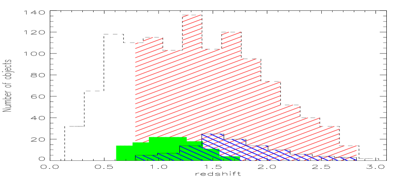
Figure 1: Redshift distributions of the population of quasars with a strong Mg ii/Fe ii absorber (solid line), the sample of absorbers (filled histogram) and the population of quasars without such absorbers (dashed line). For the latter one our analysis considers only quasars whose redshifts overlap the ones of quasars with absorbers (red dashed region). Since the probability of finding an absorber increases with redshift, the sample of quasars with an absorber presents a redshift distribution skewed towards high redshifts with respect to the reference population.

We present the redshift distributions of the three populations relevant to this study in Figure 1: the initial sample of quasars without any strong absorber (dashed line), the population of quasars with a strong Mg ii/Fe ii absorber (solid line) and the corresponding detected Mg ii/Fe ii absorbers (filled histogram). Since the probability of finding an absorber increases as a function of redshift, the redshift distribution of the sample of quasars with an absorber is skewed towards high redshifts with respect to the population of quasars without an absorber. In addition, the apparent magnitude of a quasar depends on distance as well as intrinsic luminosity. Therefore, a meaningful comparison of their magnitude distributions requires the samples to have the same redshift distribution. Thus, we will work with subsamples of the population of quasars without absorbers selected such that the number of objects and the redshift distributions are identical to that of the quasars with an absorber. This range is represented by the red dashed region in Figure 1. Moreover this choice of redshift distribution automatically rejects the low redshift quasars for which the Fe ii lines (2344, 2382, 2587 and 2600 Å) do not fall in the observed wavelength range. This set of bootstrapped subsamples constitutes our reference sample.

2.1.3 Signal-to-noise Properties

The absorber detection efficiency depends on the S/N of the quasar spectra, so it is necessary to verify how this parameter influences the magnitude distribution of the two quasar populations. Since each field observed by the 2QZ was exposed approximately for the same length of time (about 55 minutes), we expect some correlation between the magnitude of the quasars and their S/N.

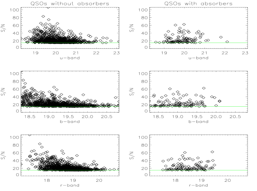
Figure 2: Magnitude-S/N distributions of the two quasar populations in u-, b- and r-bands. The reference population is plotted on the left hand side and the population of quasars with a detected absorber on the right hand side. A correlation is clearly seen in each band. The S/N parameter is the one given by the 2dF, i.e. computed in the range 4000-5000Å . The horizontal light-coloured line defines the limit S/N$>$15 used by Outram et al. (2001) in order to define the quasar sample.

In Fig. 2, we plot the 2dF S/N estimate as a function of the magnitude of the quasars in the u-, b- and r-bands. The right panels show the population of quasars with a detected absorber and the left ones the reference population. Bright quasars tend to have higher S/N as is expected; the scatter of this correlation is quite large since the S/N not only depends on magnitude, but also on the sky brightness, the exposure time and the air mass. Given this correlation, it is important to check that the absorber selection does not bias the sample towards a preferential range of S/N and hence biases the magnitudes.
In a spectrum with a resolution FWHM, the minimum detectable equivalent width with a $n\sigma$ significance is:

$${\rm W_{min}}=n\times{\rm FWHM}\times{\rm(S/N)^{-1}}\;,$$ (1)

Given the resolution of 2dF spectra (FWHM = 8Å), the minimum equivalent width detectable at 5$\sigma$ for a S/N greater than 15 is W${}_{\rm{min}}=2.6$Å .
The visual detection of Mg ii/Fe ii systems is mostly based on the Mg ii absorption feature, since the Mg ii doublet is the more distinct feature (see Figure 4 for an example). The equivalent widths of the Mg ii absorbers we use are given by Outram et al. (2001, see Table 1 of their paper). In Fig. 3 we show the distribution of the observed Mg ii equivalent widths as a function of spectrum’s S/N with triangles. Following Eq. 1, the solid line represents the region above which Mg ii absorbers can be detected at least at the 5$\sigma$ level. Since all the absorbers lie above the solid line of this figure, all of them have a sufficient detection level ($>5\sigma$) to be identified in any of the quasar spectra of the sample. Therefore, based on the Mg ii absorption line detection, our sample is not biased towards any preferential S/N or magnitude range.

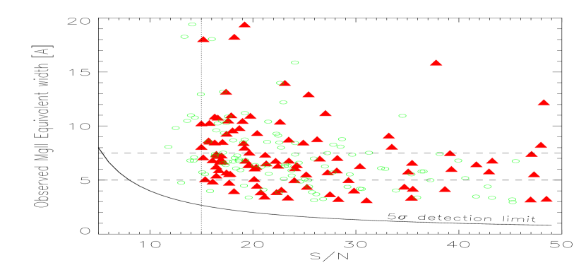
Figure 3: Observed Mg ii equivalent width W as a function of spectrum S/N. The typical uncertainty on W is of the order of 20 per cent. The solid line indicates the region above which Mg ii absorbers are detected at more than 5$\sigma$. The triangles show the 2dF S/N estimate based in the 4000-5000 Å range and the circles show our estimate using the 5000-7000 Å range. The two horizontal lines represent the lower limits used in section 3 to discard possible biases in the absorber detection procedure. Note that five systems with S/N$>$50 are not displayed for clarity.

The fact that all the points lie well above the $5\sigma$ level depends on the criteria used by Outram et al. (2001) in their absorber search (for example the requirement of the presence of Fe ii lines) and show that only very robust detections are considered. We have further checked this by visually inspecting the spectra of the objects listed by Outram et al. and found that most of the systems show the four Fe II lines (2344, 2382, 2587 and 2600 Å) and all of them clearly show at least three of the four lines. The simultaneous detection of several lines (in addition to the presence of Mg ii) makes the Fe ii detection quite robust.

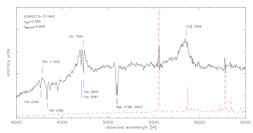
Figure 4: Example of Mg ii/Fe ii detection. The spectrum of this quasar at $z_{\rm em}=2.06$ clearly shows the Mg ii doublet as well as the four Fe ii lines expected for an absorber at $z_{\rm abs}=0.82$. This spectrum has a signal-to-noise ratio of 48. The dashed line is the corresponding sky spectrum.

Besides, it is worth pointing out that given the rest frame wavelengths of Mg ii transitions (2796 and 2803Å), a number of the corresponding absorption lines fall in the range 5000-7000Å of the quasar spectra. However, as mentioned above, the S/N-parameters as determined by the 2QZ team are measured in the range 4000-5000Å. Since the S/N of a spectrum is a function of the observed wavelength, the 2QZ S/N may not be optimal for testing how the absorber detection technique might bias the luminosity function of our two quasar populations. In order to obtain a S/N parameter that more directly describes this selection bias, we have recomputed the S/N of each quasar in the observed wavelength range 5000-7000Å by using the ratio between the raw and smoothed spectra. Appropriate masks have been used at a number of locations where sky lines were not completely subtracted during data reduction.
The circles in Figure 3 show the distribution of the observed Mg ii equivalent widths as a function of our spectrum’s S/N estimator made in the range 5000-7000Å . The fact that all the circles lie also above the solid line shows that the Mg ii absorber detection is not biased towards any preferential S/N in the whole 4000-7000Å range of the spectra.

3 The effect of absorbers on the quasar magnitude distribution

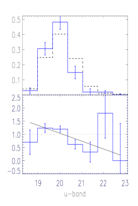
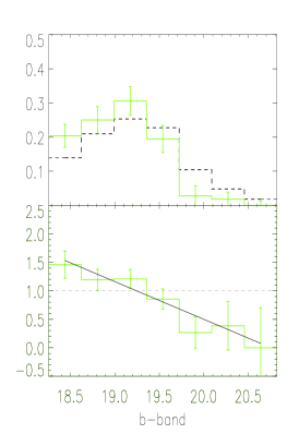
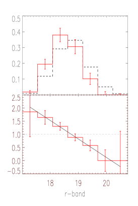
Figure 5: The top panels present the u-, b- and r-band magnitude distributions of the population of quasars with a strong Mg ii/Fe ii absorber in solid lines and the quasars without such absorbers in dashed lines. The latter is computed from a combination of bootstraps that match the redshift distribution of the first. The bottom panels show the distribution ratios, as well as noise coming from the finite size of the small sample of quasars with an absorber. Each magnitude band clearly indicates a tilt between the two magnitude distributions.

Now we compare the magnitude distributions of the two quasar populations, knowing that a difference can only be related to the presence of the absorber along the quasar line-of-sight.
We proceed as follows: from the reference quasar population we bootstrap $10\,000$ subsamples having the same size as the sample with absorbers, i.e. N${}_{\mathrm{QSO}}=108$ (see Table 3 for the successive steps of the object selection). As previously mentioned, the objects are chosen from the reference sample with the same redshift distribution as the sample with absorbers. The combined 10 000 bootstrap samples without absorbers are used as a reference sample in what follows.

In the upper panels of Fig. 5 we show the magnitude distribution of the two quasar samples in the u-, b- and r-bands. The solid line represents the magnitude distribution of the quasars with an absorber and the dashed line shows the combined reference sample. Since these two populations have different sizes, we plot the fraction of objects per magnitude bin. The magnitude distribution of quasars with an absorber appears to be skewed towards bright objects with respect to the reference population. This effect is observed in each band and suggests an intrinsic difference in the magnitude distributions. We now show that this difference is significant: we estimate the Poisson noise associated with the number of quasars with absorbers per magnitude bin $N_{\mathrm{QSO+abs}}(m)$ by computing the r.m.s. deviations in each bin of the bootstrap subsamples introduced above. We neglect the noise contribution of the reference population $N_{\mathrm{QSO,ref}}$, i.e. the combined bootstraps, since it is a much larger sample. For each band, we compute the ratio between the two magnitude distributions: $N_{\mathrm{QSO+abs}}(m)/N_{\mathrm{QSO,ref}}(m)$, normalised by the number of objects. The ratios are displayed in the lower panels of Fig. 5. Each of them is then fitted by a straight line with gradient $\gamma$. If both samples had similar distributions, then the ratio would be unity and $\gamma$ would be zero. However, in each band, these fits indicate a tilt between the two magnitude distributions, showing an excess of bright (and/or a deficit of faint) quasars with an absorber with respect to the reference population. The corresponding gradients are $\gamma_{u}=-0.29\pm 0.12$, $\gamma_{b}=-0.66\pm 0.17$ and $\gamma_{r}=-0.70\pm 0.15$ in the u, b, and r bands, respectively. The significance of these detection is computed by applying the same analysis to the 10 000 bootstrapped samples, i.e. we compare each of them to the combined reference population, by computing the corresponding ratios and fitting them with straight lines. Fig. 6 shows the corresponding distribution of gradients $\gamma_{\mathrm{boot}}$ for each band, as well as the value found for the sample of quasars with absorbers (vertical line). Each distribution is well fitted by a Gaussian. It appears that the magnitude distribution of the quasars with absorber significantly deviates from the magnitude distributions of random reference samples. Bright quasars with an absorber are in excess compared to the reference population (and/or faint quasars are in deficit). The tilt between the two populations is seen at the 2.4, 3.7 and 4.4$\sigma$ level in the u-, b- and r-bands respectively. Table 1 summarizes the amplitude of these detections. Note that these values are relatively weakly sensitive to the number of bins used.

Given the fact that we fix the number of quasars in the bootstrap subsamples to match the number of quasars with an absorber, the only relevant information in our comparison is the value of the tilt, i.e. the gradient $\gamma$ between the magnitude distributions. The magnitude for which the two distributions are similar (the zero point) can not be estimated with this technique and therefore the observed tilt could arise either from an excess of bright quasars with an absorber, or from a deficit of faint quasars with absorbers, or from a combination of the two. This analysis shows, that the magnitude distributions and therefore the number counts of quasars with such Mg ii/Fe ii absorbers are significantly different from the ones of similar quasars without such absorption lines. Equivalently, more absorbers are found in front of bright quasars.

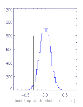
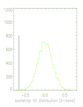
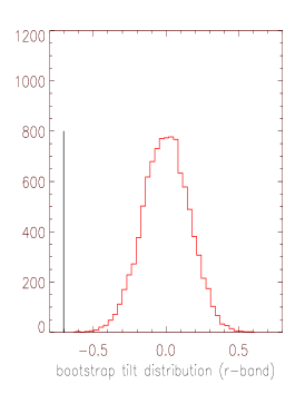
Figure 6: Distributions of the gradients $\gamma_{\mathrm{boot}}$ obtained by fitting the ratio between the 10 000 bootstraps subsamples and the combined reference sample, in u-, b- and r-bands. The scatter of these distributions allows us to define the significance levels of the tilt detection for the sample of quasars with an absorber. These detections are shown with the vertical lines.

In order to further discard the existence of biases towards any preferential S/N during the absorber detection technique (which we note was based on a visual inspection), we have also performed our analysis on two subsamples of Mg ii/Fe ii absorbers having observed equivalent widths $W_{obs}>5.0$ and $W_{obs}>7.5$ Å. Indeed, the greater the observed equivalent widths are, the more robust their detection in spectra are. The corresponding results are presented in Table 1. As we can see, the signals for the larger equivalent widths subsamples show gradients that are consistent with the main sample. This test strengthens the interpretation that biases in the absorber detection procedure are not responsible for the differences measured in the magnitude distributions, and that the relative excess of bright quasars with an absorber is real.

Main sample: 108 QSO with abs.

band gradient $\gamma$ detection level u -0.29$\pm 0.12$ 2.4$\sigma$ b -0.66$\pm 0.17$ 3.7$\sigma$ r -0.70$\pm 0.15$ 4.4$\sigma$

$\mathrm{W}_{obs}>5.0$ Å   83 QSO with abs.

band gradient $\gamma$ detection level u -0.35$\pm 0.14$ 2.3$\sigma$ b -0.62$\pm 0.19$ 3.0$\sigma$ r -0.65$\pm 0.17$ 3.5$\sigma$

$\mathrm{W}_{obs}>7.5$ Å   37 QSO with abs.

band gradient $\gamma$ detection level u -0.28$\pm 0.21$ 1.2$\sigma$ b -0.78$\pm 0.29$ 2.5$\sigma$ r -0.90$\pm 0.25$ 3.3$\sigma$

Table 1: This table lists the gradient $\gamma$ of the ratio between the magnitude distribution of the quasars with an absorber and the reference population, as well as the significance level of a non-constant ratio ($\gamma$=0), for each magnitude band. These significance values come from the 10 000 bootstrap subsamples (see Fig 6).

4 Interpretation

Given that the selection procedure of the two quasar populations discards biases with magnitude, the observed differences must be related to the presence of absorbers. Indeed, such a structure along the line-of-sight of a quasar can modify the quasar magnitude in different ways. Firstly, the presence of dust in the absorber could cause some extinction and redden the quasar light. Secondly, if the absorber is a galaxy it could also contribute to the observed luminosity of the quasar. Thirdly, if this absorber system is sufficiently massive it can gravitationally lens the background quasar and so modify its magnitude. Finally, a fraction of the absorbers could be physically associated with the quasars and therefore correlate with their physical properties and orientations. In this section, we review these effects and estimate their impact on the quasar magnitude distribution.

4.1 Obscuration effects

Absorber systems are believed to contain dust which produces extinction effects on the background quasar (Pei & Fall 1995). This phenomenon is wavelength-dependent: bluer parts of the spectrum are more affected, rendering the absorption-line sample to appear redder than the reference one.

Extinction effects will shift the quasar magnitude distribution to fainter magnitudes. Given the shape of these distributions in our case (see Fig. 5), extinction effects should increase the number of faint quasars and thus tilt the magnitude distribution of the quasars with an absorber to a positive gradient $\gamma$. In contrast, we detected the opposite effect in the previous section, i.e. a negative gradient. This implies the existence of a phenomenon related to the absorber whose amplitude is opposite to and dominates over extinction effects.

Besides, we note that since extinction effects are expected to be stronger in bluer bands, this could well explain the lower amplitude of the tilt observed in the u-band compared to the r-band.

4.2 Flux Contribution from the Absorber

It is believed that the systems responsible for the Mg ii/Fe ii absorptions observed in the background quasar spectra might be associated with galaxies. If these galaxies are bright enough and if the impact parameter is small enough, they could contribute to the magnitudes measured for the quasars. The contribution to the ratio between the apparent luminosity distributions of the quasars with and without absorbers is:

$$R(l_{QSO}^{obs})=\frac{l_{QSO}+l_{absorber}}{l_{QSO}}\,.$$ (2)

Therefore this effect would increase the relative number of faint quasars with respect to the number of bright ones. It would therefore give rise to a positive gradient $\gamma$, as opposed to the negative values observed in the previous section.
It is known from deep observations of both DLAs and Mg ii systems (Le Brun et al. 1997; Boissé et al. 1998; Bergeron & Boissé 1991) that the luminosity of these objects is small. Thus, the flux contribution of the absorber to the quasar luminosity is probably small in general. Moreover, absorbers are located at various redshifts and have different luminosities. Since these parameters are uncorrelated with the properties of the background quasar, such effects should further reduce the absorber flux contribution to the global magnitude distribution.

4.3 Gravitational Lensing

Under the assumption that the absorber systems are intervening galaxies along the lines-of-sight, a likely explanation for the observed trend in the magnitude distributions is the magnification bias due to gravitational lensing. Indeed, gravitational magnification has two effects:

• first, the flux received from background quasars is increased by a magnification factor $\mu$ which is related to the overdensities of matter along their line-of-sight;

• on the other hand, the solid angle in which sources appear is stretched. The probability of observing such quasars is reduced.

Additionally, a ’by-pass’ effect causes the lines-of-sight towards background quasars to avoid the central parts of galaxies and reduces their effective cross-section for absorption.

Considering the first effects, the relative change in the number of quasars with absorbers depends on the magnification factor $\mu$ and the shape of the quasar magnitude distribution. Indeed, this effect shifts the magnitude distribution of the background sources towards brighter values. The steeper the number counts, the higher the increase. The number of sources with a steep luminosity function, like bright quasars, will be increased. On the other hand if the local number counts decreases as a function of magnitude, the corresponding number of lensed quasars is reduced. As we show now, this effect depends on the magnification factor $\mu$ and the gradient of the number of sources as a function of magnitude. Let $\mathrm{n_{0}}(s)\,\mathrm{d}s$ be the number of unlensed quasars with a flux in the range $[s,s+\mathrm{d}s]$ and $\mathrm{n}(s)\,\mathrm{d}s$ the corresponding number of lensed quasars. Let’s write the unlensed source counts as

$$\mathrm{n_{0}}(s)\,\mathrm{d}s = a\,s^{-\beta(s)}\,\mathrm{d}s\,.$$ (3)

The magnification effect will enlarge the sky solid angle, thus modifying the source density by a factor $1/\mu$, and at the same time increase their fluxes by a factor $\mu$. These effects act as follows on the number of lensed sources:

$$\mathrm{n}(s)\,\mathrm{d}s = \mathrm{Prob}(\mu)\times\frac{1}{\mu}\;\mathrm{n_{0}}\,(\frac{s}{\mu})\;\frac{\mathrm{d}s}{\mu}$$ (4)

$$= \mathrm{Prob}(\mu)\times\mu^{-2}\,a\,\left(\frac{s}{\mu}\right)^{\beta(s/\mu)}\,\mathrm{d}s$$

where Prob$(\mu)$ is the probability of having a lens with magnification $\mu$ giving rise to the absorption lines of interest in the quasar spectrum. This coefficient plays only the role of a normalisation factor. If $\beta$ does not vary appreciably over the interval $[s,s/\mu]$, which is well satisfied if $\mu$ departs weakly from unity, then

$$\mathrm{n}(s) \approx \mathrm{Prob}(\mu)\times\mu^{\beta(s)-2}\,n_{0}(s)$$ (5)

which can be written as a function of magnitude as

$$\mathrm{n}(m)\, \approx \mathrm{Prob}(\mu)\times\mu^{2.5\;\beta(m)-1}\,\mathrm{n_{0}}(m)$$ (6)

where $\beta(m)=\mathrm{d}\log[\mathrm{n}_{0}(m)]\,/\,\mathrm{d}m$. The final effect, i.e. a relative excess or deficit of lensed quasars with a magnitude $m$, is then controlled by the value of $\beta(m)$. We have computed this quantity using the values of $\mathrm{n}_{0}(m)$ given by the sample of reference (i.e. unlensed) quasars introduced above. The results are plotted in in Fig. 7. As we can see, it indicates that the magnification bias would give rise to a relative excess of bright quasars with absorbers whereas faint quasars are depleted. Here we note also that the magnification bias is chromatic since the $\beta$ value depends on the observed wavelength. In some cases, such an effect can thus introduce some correlations between the absorbers and the quasar magnitudes, colours, spectral index for example.

The additional effect mentioned above, the by-pass effect, is detailed in Smette et al. (1997) and Bartelmann & Loeb (1995). It systematically reduces the number of observable high-equivalent widths absorption lines for impact parameters smaller than the Einstein radius of the lens and is independent on the magnitude of the background sources.

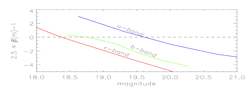
Figure 7: The value of $2.5\times\beta(m)-1$ is shown as a function of magnitude in the u-, b- and r-bands and indicate the relative excess of bright quasars with absorbers expected from the magnification bias. Note that the three bands span different magnitude ranges.

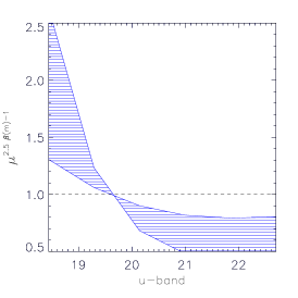
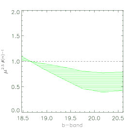
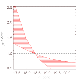
Figure 8: The value of the gravitational magnification bias $\mu^{2.5\beta(m)-1}$ is plotted as a function of magnitude, for the u-, b- and r-bands. The amplification $\mu$ depends on the lens properties and the coefficient $\beta$ is the logarithmic slope of the reference quasar number counts (see Fig. 7). As described by Eq. 6 this quantity is proportional to the expected ratio between the number of quasars with and without absorbers as a function of magnitude. We are considering here a simplified model with amplifications ranging from $\mu=$1.07 to 1.3, as motivated in the text. The overall gradients given by this magnification bias are comparable to the one observed from the data. Note that the amplitudes can not be compared given the need of normalizing the samples.

In order to illustrate that the lensing explanation is in quantitative agreement with our measurements we consider now a simplified scenario and compute the corresponding lensing effects. For estimating the amplification $\mu$ we assume the dark matter distribution of the absorbers to be isothermal with a velocity dispersion between 100 and 200 $\mathrm{km\,s^{-1}}$ as it is expected for spiral galaxies. For a quasar at $z=2$, an absorber at $z=1$ and an effective impact parameter of 10 kpc (following the spatial distribution given by Steidel (1993) for DLAs) we find an amplification $1.07\lesssim\mu\lesssim 1.3$ for $\Omega_{m}=0.3$ and $\Omega_{\Lambda}=0.7$. The impact parameter being a few times larger than the Einstein radius of the lens, the by-pass effect becomes rather weak (see Fig. 3 in Smette et al. 1997) and can be neglected in the following. Therefore the total magnification bias is simply described by Eq. 6. Using the values of $\beta(m)$ introduced above, we plot $\mu^{2.5\beta(m)-1}$ in Fig. 8 for the three different bands. The corresponding curves describe the relative excess of quasars with an absorber and are therefore directly related to the lower panels of Fig. 5. Our simplified model does not aim at reproducing the exact amplitude and shape of expected lensing effects. It is only an indication of the magnification bias behaviour. As we can in Fig. 8, it shows that the overall gradients obtained from gravitational lensing are similar to the ones measured from the data in the previous section (note that the amplitudes cannot be compared in a straightforward manner contrary to the gradients). This quantitative result strengthens the evidence towards gravitational lensing being at the origin of the tilt measured in this study. It also shows how the signal found in section 3 is related to the average magnification due to absorber halos and can therefore constrain their mass distribution.

More detailed calculations taking into account the redshift distributions of the quasars and the absorbers as well as a distribution of impact parameters and the inclusion of the by-pass effect are beyond the scope of this paper; but they will be required in the future in order to estimate the expected lensing effects more accurately and to infer some constraints from such observations on the potential wells of these systems.

4.4 Intrinsic Absorbers

Despite the fact that intervening galaxies are clearly at the origin of some absorption lines, a number of our absorber systems may actually be physically associated to the quasars. Such associations have been confirmed when broad absorption lines are seen in quasar spectra (Turnshek 1988, Weymann 1997) but the situation is still unclear in the case of narrow lines (Borgeest & Mehlert 1993). Recently, Richards et al. (1999, 2001) and Richards (2001) observed correlations between quasar properties (magnitude, spectral index) and the number of absorbers found in their spectra. They suggested that the presence of absorbers might be related to the orientation of the quasars and thus gives rise to some correlations with quasar magnitudes.

To investigate whether associations could be responsible for the magnitude differences observed in section 3, we have redone our analysis for subsamples of absorbers with different escape velocities. Indeed, associations can no longer be at the origin of observed correlations when the velocity difference between a quasar and a metal absorber is a substantial fraction of the speed of light.

Figure 9: Distribution of absorber escape velocities. The vertical lines located at 45 000 and 90 000 km/s indicate the limits used for the two low and high escape-velocity subsamples.

Figure 9 shows the distribution of the blueshifted absorber velocities relative to the emission-line redshift of the QSOs, given by:

$$\beta=\frac{v}{c}=\frac{(1+z_{\mathrm{QSO}})^{2}-(1+z_{\mathrm{abs}})^{2}}{(1+z_{\mathrm{QSO}})^{2}+(1+z_{\mathrm{abs}})^{2}}\,.$$ (7)

In order to see how the signal varies as a function of $\beta$ we analyse two subsamples of the same size: one with escape velocities $v>90\times 10^{3}\,\hbox{km s${}^{-1}$}$, i.e. for which associations can hardly be invoked, and a corresponding low-escape velocity sample with $v<45\times 10^{3}\,\hbox{km s${}^{-1}$}$. Each sample has 39 systems. The results are summarized in Table 2 where we present the values of the gradients $\gamma$ and their significance, for the u-, b- and r-bands. The size of these subsamples being reduced by almost a factor three compared to the measurement performed in section 3, it is expected to have significantly lower detection levels. Nethertheless we can observe that the signal can be detected in each case at the $2\sigma$ level at least. Within the accuracy we can reach, the $\gamma$ values do not show any specific trend with escape velocity.

Low escape velocity $v<45\times 10^{3}$km/s 39 QSO with abs.

band gradient $\gamma$ detection u -0.41$\pm 0.20$ 1.9$\sigma$ b -0.88$\pm 0.27$ 3.2$\sigma$ r -0.74$\pm 0.25$ 2.9$\sigma$

Medium escape velocity $v>90\times 10^{3}$km/s 39 QSO with abs.

band gradient $\gamma$ detection u -0.47$\pm 0.21$ 2.0$\sigma$ b -0.67$\pm 0.27$ 2.2$\sigma$ r -0.57$\pm 0.24$ 2.2$\sigma$

Table 2: Values of the gradients $\gamma$ found for absorber subsamples of different escape velocity ranges. At low escape velocities, either gravitational lensing or physical associations might be able to give rise to negative $\gamma$ values, whereas only lensing seems to be able to be at the origin of the effect found for the high-escape velocity sample.

For the low-escape velocity sample the detection of the tilt could arise either from correlations due to associated absorbers, as suggested by Richards et al. (1999, 2001), or from gravitational lensing effects. In this case, each scenario is plausible. However, the detection of the tilt for the high-escape velocity sample can hardly be explained by associations since this case deals with velocities higher than roughly one third of the light speed. Therefore, for this subsample, we can fully attribute the excess of bright (and/or deficit of faint) quasars with an absorber to gravitational lensing effects.

Since such a lensing signal contains valuable information about the gravitational potential of the absorbers, it would be of great interest to estimate the fraction of associated absorbers as a function of escape velocity. This will allow us to maximise the number of quasars for which only lensing induced correlations are expected and therefore improve the accuracy of the magnification bias measurement.

5 Conclusion

Using the first release of the 2dF Quasar survey (2QZ), we have looked for the magnification bias due to intervening absorption systems along the line-of-sight of quasars. Contrarily to previous studies which searched changes in quasar magnitudes due to presence of numerous but weak absorbers in quasar spectra, we have focused on the strongest absorption systems.
The 2QZ sample lists over 10 000 quasars of which 1363 were visually inspected by Outram et al. (2001) for the compilation of a strong metal absorber catalogue. Motivated by the idea that some of these systems may trace galaxies, a magnification bias is expected to modify the magnitude distribution of the corresponding background quasars (Bartelmann & Loeb 1995, Pei 1995, Perna et al. 1997, Smette et al. 1997). In order to measure such an effect, we have carefully selected samples of quasars and absorbers according to the following main steps:

• from the catalogue compiled by Outram et al. (2001) we selected the Mg ii/Fe ii absorbers. Note that these systems have $1.3\lesssim\,$W${}_{0}\,($Mg ii doublet$)\lesssim 9.0$ Å,

• for the corresponding observed equivalent widths, we have checked that the detection of these absorption lines is not biased with respect to the signal-to-noise of the spectra,

• we define a reference population by bootstrapping the population of quasars without absorber with a redshift distribution identical to the one of quasars with an absorber.

By comparing the magnitude distributions of the resulting quasar populations, we have showed that these are significantly tilted: an excess of bright (and/or a deficit of faint) quasars with an absorber is detected at the 2.4, 3.7 and 4.4$\sigma$ levels in the u, b and r-bands. Moreover a consistent signal is still detected (at the 3.3$\sigma$ in r-band) if we use only the absorbers with the highest observed equivalent widths (W$>7.5$Å), i.e. systems much less sensitive to biases in the detection procedure. Given the similar redshift and signal-to-noise properties imposed by our sample selection, this magnitude difference is necessarily related to the presence of the absorbers. This detection implies that number counts of quasars with strong Mg ii/Fe ii absorbers are substantially modified with respect to quasars without such absorbers along their line-of-sight and corrections have to be applied in order to recover the true underlying properties of these objects.

We review different effects arising when a matter concentration intercepts the light coming from a quasar: extinction and reddening, flux contributions from the absorbing system, gravitational lensing and correlations due to physical quasar-absorber associations. We argued that only the two latter explanations can give rise to the trend we observe. We have then redone our analysis on two subsamples of the same size having low ($v<45\times 10^{3}\,\hbox{km s${}^{-1}$}$) and high ($v>90\times 10^{3}\,\hbox{km s${}^{-1}$}$) quasar-absorber velocity differences. In each case we detected similar magnitude changes (at the 1.9 to 3.2$\sigma$). For the low-escape velocity sample, either gravitational lensing or physical associations could be at the origin of the observed correlation. However for the high velocity sample, the only likely explanation for the changes in the magnitude of quasars with an absorber is gravitational lensing since, in this case, the velocity differences between quasars and absorbers are greater than roughly one third of the light speed. Being able to isolate and measure such a lensing signal is of great interest since this magnification bias contains information about the absorber gravitational potential.

Our analysis also shows that the changes in quasar magnitudes due to the presence of absorbers tend to be stronger in redder bands. This trend might be explained by extinction effects since they give rise to an effect opposite to that of gravitational lensing, i.e. a relative excess of faint quasars with an absorber, which is expected to be stronger in bluer bands. Isolating gravitational lensing from extinction effects would be possible by using complete quasar samples in different bands.

The effects of the magnification bias depend on the slope of the source number-counts as a function of magnitude and therefore on the characteristics of a given survey. In the case of 2QZ quasars, the corresponding number count slopes are expected to give rise to a relative excess of bright quasars, in agreement with our detection. Moreover, we have shown that a simplified gravitational lensing model gives quantitative tilt predictions comparable to the ones observed in the magnitude distribution of quasars with absorbers. More accurate measurements of this effect might therefore give us interesting constraints on the absorber mass distribution.

It should be emphasized that such a lensing technique allows us to greatly extend the usual redshift ranges probed by existing statistical shear or magnification measurements (see Mellier 1999 for a review). Indeed, given the need of background galaxies, these previous measurements were restricted to z${}_{\rm lens}\lesssim 1$, whereas the use of quasars and absorbers allows us to easily probe lensing effects at z${}_{\rm lens}\sim$1–2. Moreover the lenses are selected according to their lensing optical depth as opposed to mass or luminosity.

We are currently undertaking a similar analysis using SDSS spectra. Using a different survey and facing different systematics will allow us to check the significance of the present detection. Besides the larger sample sizes that Sloan will provide, the better spectrum quality will allow the detection of various kinds of absorption lines. Therefore we will be able to extend the analysis to different metal absorbers and see, via the magnification bias, how they populate dark matter halos. This technique might therefore provide a promising tool to get new constrains on the nature of high-redshift absorber systems.

Appendix A The sample of quasars with Mg ii/Fe ii absorbers

This appendix gives explicitly the list of quasars with absorbers we use in our analysis. The initial sample comes from Outram et al. (2001). We refer the reader to this paper for the details about the compilation of this catalogue, as well as more information on each system.

Table 3 summarises the main steps we used in order to select our sample of quasars with strong Mg ii/Fe ii absorbers. A detailed list of the corresponding objects is given in Table 4. From the list of quasars with Mg ii/Fe iiabsorbers given by Outram et al., we do not take into account two systems in our analysis: the first one (flagged R1) is a quasar not detected in the r-band. The second one (flagged R2) has an absorber escape velocity smaller than $3\,000$ km/s.
The A flag indicates the presence of two absorbers in the quasar spectrum and the B flag is used when one of these two absorbers has $z_{\rm{abs}}\approx z_{\rm{QSO}}$.

Table 3: Summary of the successive steps of the sample selection with the corresponding number of quasars.

	reference	quasars with
Selection criteria	quasars	absorber
1. Initial catalogue from Outram et al.	1135	129
(2001)
2. Selecting only quasars with Mg ii	1135	110
and Fe ii systems
3. Excluding quasars not detected	1114	109
in the r-band
4. Rejecting associated absorbers	1114	108
with $\Delta v<3000$ km/s

Table 4: Detailed list of the quasars with an absorber used in our analysis.

Quasar	$z_{\rm em}$	S/N	$z_{\rm abs}$	W0	Flag
J000534.0-290308	2.347	19	1.168	4.83
J000811.6-310508	1.683	25	0.715	2.55
J001123.8-292500	1.280	20	0.605	6.82
J001233.1-292718	1.565	16	0.913	2.83
J002832.4-271917	1.622	47	0.753	1.83
J003142.9-292434	1.586	23	0.930	5.39
J003533.7-291246	1.492	17	1.457	3.78
J003843.9-301511	1.319	43	0.979	2.93
J004406.3-302640	2.203	22	1.042	3.10
J005628.5-290104	1.809	23	1.409	3.63
J011102.0-284307	1.479	26	1.156	3.24
J011720.9-295813	1.646	36	0.793	2.53	R1
J012012.8-301106	1.195	64	0.684	4.01
J012315.6-293615	1.423	16	1.113	2.30
J013032.6-285017	1.670	16	1.516	3.37
J013356.8-292223	2.222	17	0.838	4.64

Quasar	$z_{\rm em}$	S/N	$z_{\rm abs}$	W0	Flag
J013659.8-294727	1.319	17	1.295	3.01
J014729.4-272915	1.697	15	0.811	3.92
J014844.9-302817	1.109	49	0.867	1.75
J015550.0-283833	0.946	35	0.677	2.62
J015553.8-302650	1.512	16	1.316	3.18
J015647.9-283143	0.919	17	0.884	3.14
J015929.7-310619	1.275	28	1.079	1.56
J021134.8-293751	0.786	18	0.616	3.45
J021826.9-292121	2.469	19	1.205	4.45
J022215.6-273231	1.724	23	0.611	2.55
J022620.4-285751	2.171	18	1.022	9.03
J023212.9-291450	1.835	15	1.212	4.63	A
J024824.4-310944	1.399	26	0.789	4.91	A, B
J025259.6-321125	1.954	17	1.735	3.94a
J025608.0-311732	1.255	33	0.973	4.62	A
J025919.2-321650	1.557	16	1.356	3.15
J030249.6-321600	0.898	48	0.821	4.54
J030324.3-300734	1.713	42	1.190	2.95
J030647.6-302021	0.806	21	0.745	4.21
J030711.4-303935	1.181	25	0.966	2.81	A, B
J030718.5-302517	0.992	25	0.711	4.95
J030944.7-285513	2.117	21	0.931	3.39
J031255.0-281020	0.954	15	0.955	2.06	R2
J031309.2-280807	1.435	21	0.950	1.78
J031426.9-301133	2.071	25	1.128	6.08	A
J095605.0-015037	1.188	20	1.045	3.04
J095938.2-003501	1.875	27	1.598	4.31
J101230.1-010743	2.360	17	1.370	2.83
J101556.2-003506	2.462	17	1.489	2.29
J101636.2-023422	1.519	18	0.912	2.90
J101742.3+013216	1.457	18	1.313	1.72a
J102645.2-022101	2.401	23	1.581	1.31
J105304.0-020114	1.527	16	0.888	5.76
J105620.0-000852	1.440	22	1.285	1.70
J110603.4+002207	1.659	36	1.018	2.08
J110736.6+000328	1.726	51	0.953	2.65
J114101.3+000825	1.573	17	0.841	3.93
J115352.0-024609	1.835	20	1.204	2.90
J115559.7-015420	1.261	19	1.132	3.75
J120455.1+002640	1.557	16	0.597	3.92
J120826.9-020531	1.724	20	0.761	5.31
J120827.0-014524	1.552	15	0.621	3.13
J120836.2-020727	1.081	27	0.873	1.97
J122454.4-012753	1.347	20	1.089	2.14
J125031.6+000216	2.100	20	1.327	2.61
J125658.3-002123	1.273	28	0.947	3.62
J130019.9+002641	1.748	17	1.225	5.92
J130433.0-013916	1.596	19	1.410	8.05
J130622.8-014541	2.152	16	1.332	3.67
J133052.4+003219	1.474	52	1.327	1.89
J134448.0-005257	2.083	18	0.932	5.44
J135941.1-002016	1.389	30	1.120	2.97
J140224.1+003001	2.411	24	1.387	2.85
J140710.5-004915	1.509	16	1.484	3.49
J141051.2+001546	2.598	16	1.170	4.74
J144715.4-014836	1.606	18	1.354	2.02
J214726.8-291017	1.678	35	0.931	1.74
J214836.0-275854	1.998	55	1.112	1.40
J215024.1-282508	2.655	30	1.144	1.88

Quasar	$z_{\rm em}$	S/N	$z_{\rm abs}$	W0	Flag
J215034.6-280520	1.358	35	1.139	1.58
J215222.9-283549	1.228	24	0.927	2.59
J215342.9-301413	1.729	31	1.037	1.54
J215359.0-292108	1.160	22	1.036	3.33
J215955.4-292909	1.477	23	1.241	6.24
J220003.0-320156	2.047	16	1.135	3.20
J220137.0-290743	1.266	24	0.600	3.81
J220208.5-292422	1.522	47	1.490	2.98
J220214.0-293039	2.259	78	1.219	3.39
J220655.3-313621	1.550	15	0.754	4.60
J221155.2-272427	2.209	35	1.390	2.76
J221546.4-273441	1.967	20	0.785	2.86
J222849.4-304735	1.948	33	1.094	3.86
J223309.9-310617	1.702	47	1.146	2.58
J224009.4-311420	1.861	29	1.450	2.04b
J225915.2-285458	1.986	18	1.405	4.57
J230214.7-312139	1.699	21	0.955	1.98
J230829.8-285651	1.291	43	0.726	3.94
J230915.3-273509	2.823	18	1.060	4.66
J231227.4-311814	2.743	20	1.555	2.95
J231459.5-291146	1.795	39	1.402	3.12
J232023.2-301506	1.149	17	1.078	3.50
J232330.4-292123	1.547	17	0.811	3.70
J232700.2-302637	1.921	38	1.476	6.41	A
J232914.9-301339	1.494	20	1.294	2.78
J232942.3-302348	1.829	15	1.581	6.99
J233940.1-312036	2.611	27	1.444	2.34
J234321.6-304036	1.956	28	1.052	2.87
J234400.8-293224	1.517	35	0.851	3.13
J234405.7-295533	1.705	19	1.359	2.88
J234527.5-311843	2.065	48	0.828	6.67
J234550.4-313612	1.649	39	1.138	1.95
J234753.0-304508	1.659	39	1.421	2.49
J235714.9-273659	1.732	24	0.814	3.52
J235722.1-303513	1.910	19	1.309	3.65

^a Rest equivalent width of Fe ii $\lambda$=2600 Å (Mg ii blended with sky lines)
^b Rest equivalent width of Mg ii $\lambda$=2796 Å only.

References

- (1) Bartelmann, M. & Loeb, A., 1995, ApJ, 457, 529
- (2) Bergeron, J. & Boisse, P., 1991, A&A, 243, 344
- (3) Bergeron, J., Petitjean, P., Sargent, W. L. W., Bahcall, J. N., Boksenberg, A., Hartig, G. F., Jannuzi, B. T., Kirhakos, S., Savage, B. D., Schneider, D. P., Turnshek, D. A., Weymann, R. J. & Wolfe, A. M., 1994, ApJ, 436, 33
- (4) Boisse, P., Le Brun, V., Bergeron, J., & Deharveng, J.-M., 1998, A&A, 333, 841
- (5) Boissier, S., Péroux, C. & Pettini, M., 2003, MNRAS, 338, 131
- (6) Borgeest, U. & Mehlert, D., 1993, A&A 275, L21
- (7) Boyle, B. J., Shanks, T., Croom, S. M., Smith, R. J., Miller, L., Loaring, N., Heymans, C., 2000, MNRAS 317, 1014
- (8) Broadhurst, T. J., Taylor, A. N. & Peacock, J. A., 1995, ApJ, 438, 49
- (9) Charlton, J. C. & Churchill, C. W., 1996, ApJ, 465, 631
- (10) Churchill, C. W., Rigby, J. R., Charlton, J. C. & Vogt, S. S., 1999, ApJS, 120, 51
- (11) Croom S. M., Smith R. J., Boyle B. J., Shanks T., Loaring N. S., Miller L., Lewis I. J., 2001a, MNRAS, 322, L29
- (12) Guillemin, P. & Bergeron, J., 1997, A&A, 328, 499
- (13) Hoyle, F, Outram, P. J., Shanks, T., Croom, S. M., Boyle, B. J., Loaring, N. S., Miller, L., Smith, R. J., 2002, MNRAS 329, 336
- (14) Le Brun, V., Bergeron, J., Boisse, P. & Deharveng, J.-M., 1997, A&A, 321, 733
- (15) Le Brun, V., Viton, M. & Milliard, B., 1998, A&A, 340, 381
- (16) Le Brun, V., Smette, A., Surdej, J. & Claeskens, J.-F., 2000, A&A 363, 837L
- (17) Maller, A. H., Kolatt, T. S., Bartelmann, M. & Blumenthal, G. R., 2002, ApJ, 569, 72
- (18) Mellier, Y., 1999, Annu. Rev. Astron. Astophys., 37, 127
- (19) Milliard, B., Martin, C., Bianchi, L., Byun, Y.-I., Donas, J., Heckman, T., Lee, Y.-W., Madore, B., Malina, R., Friedman, P., Rich, M., Schiminovich, D., Siegmund, O., Szalay, A.S., 2001, proceedings of “Mining the Sky, the MPA/ESO/MPE Workshop”
- (20) Mo, J. H. & Miralda-Escudé, J., 1996, ApJ, 469, 589
- (21) Narayan, R., 1989, ApJL, 339, L53
- (22) Nestor, D. B., Rao, M. S. & Turnshek, D. A., 2002, ”The IGM/Galaxy Connection” (astro-ph/0211295)
- (23) Outram, P. J., Smith, R. J., Shanks, T., Boyle, B. J., Croom, S. M., Loaring, N. S. & Miller, L., 2001, MNRAS, 328, 805
- (24) Péroux, C., McMahon, R. G., Storrie-Lombardi, L. J. & Irwin, M., 2002, MNRAS, submitted (astro-ph/0107045)
- (25) Pei, Y. C., 1995, ApJ, 440, 485
- (26) Pei, Y. C. & Fall, M. S., 1995, ApJ, 454, 69
- (27) Perna, R., Loeb, A & Bartelmann, M., 1997, ApJ 448, 550
- (28) Rao, S. M. & Turnshek, D.A., 2000, ApJS, 130, 1
- (29) Rao, S. M., Turnshek, D.A., & Briggs, F.H., 1995, ApJ, 449, 488
- (30) Richards, G. T., 2001, ApJS,133, 53
- (31) Richards, G. T., Laurent-Muehleisen, S. A., Becker, R. H. & York, D. G., 2001, ApJ, 547, 635
- (32) Richards, G. T., York, D. G., Yanny, B., Kollgaard, R. I., Laurent-Muehleisen, S. A., vanden Berk, D. E. et al., 1999, ApJ, 513, 576
- (33) Schneider, P., Ehlers, J. & Falco, E.E., 1992, Gravitational Lensing
- (34) Smette, A., Claeskens, J. F. & Surdej, J., 1997, New Astronomy 2, 53
- (35) Srianand, R. & Petitjean, P., 2000, A&A, 357, 414
- (36) Steidel, C. C. & Sargent, W. L. W., 1992, ApSS, 80, 1
- (37) Steidel, C. C., 1993, in ASSL Vol. 188; The Environment and Evolution of Galaxies, p263
- (38) Steidel, C. C., Dickinson, M. & Persson, S. E., 1994, ApJ, 437, L75
- (39) Steidel, C. C. 1995, astro-ph/9509098
- (40) Storrie-Lombardi, L. J., McMahon, R. G. & Irwin, M., 1996, MNRAS, 283L, 79
- (41) Storrie-Lombardi, L. J. & Wolfe, A., 2000, ApJ, 543, 552
- (42) Thomas, P. A. & Webster, R. L., 1990, ApJ, 349, 437
- (43) Turnshek, D. A. 1988, in Proc. QSO Absorption Line Meeting, ed. J. C. Blades, D. A. Turnshek & C. A. Norman (Cambridge University Press), 17
- (44) Vanden Berk, D. E., Quashnock, J. M., York, D. G. & Yanny, B., 1996, ApJ 469, 78
- (45) Weymann, R. 1997, in ASP Conf Ser. 128, Mass Ejection from Active Galatic Nuclei, Ed. N. Arav, I Shlosman & R. J. Weymann (San Francisco: ASP), 3
- (46) Wolfe, A. M., Turnshek, D. A., Smith, H. E. & Cohen, R. D., 1986, ApJS, 61, 249
- (47) Wolfe, A. M., 1988, in “QSO absorption lines: Probing the universe”, p297
- (48) York, D. G., Yanny, B., Crotts, A., Carilli, C., Garrison, E. & Matheson, L., 1991, MNRAS, 250, 24
- (49) York, D. G., and the SDSS collaboration, 2000, AJ, 120, 1579