The Mass, Baryonic Fraction, and X-ray Temperature of the Luminous, High Redshift Cluster of Galaxies, MS0451.6-0305

Abstract

We present new Chandra X-ray observations of the luminous and cosmologically-significant X-ray cluster of galaxies, MS0451.6-0305, at $z=0.5386$. Spectral imaging data for the cluster are consistent with an isothermal cluster of $(10.0-10.6)\pm 1.6$ keV, with an intracluster Fe abundance of $(0.32-0.40)\pm 0.13$ solar. The systematic uncertainties, arising from calibration and model uncertainties, of the temperature determination are nearly the same size as the statistical uncertainties, since the time-dependent correction for absorption on the detector is uncertain for these data. We discuss the effects of this correction on the spectral fitting. The effects of statistics and fitting assumptions of 2-D models for the X-ray surface brightness are thoroughly explored. This cluster appears to be elongated and so we quantify the effects of assuming an ellipsoidal gas distribution on the gas mass and the total gravitating mass estimates. These data are also jointly fit with previous Sunyaev-Zel’dovich observations to obtain an estimate of the cluster’s distance ($D_{A}=1219^{+340}_{-288}\pm 387$ Mpc, statistical followed by systematic uncertainties) assuming spherical symmetry. If we, instead, assume a Hubble constant, the X-ray and S-Z data are used together to test the consistency of an ellipsoidal gas distribution and to weakly constrain the intrinsic axis ratio. The mass derived from the X-ray data is consistent with the weak lensing mass and is only marginally less than the mass determined from the optical velocities. We confirm that this cluster is very hot and massive, further supporting the conclusion of previous analyses that the universe has a low matter density and that cluster properties have not evolved much since $z\sim 0.5$. Furthermore the presence of iron in this high redshift cluster at an abundance that is the same as that of low redshift clusters implies that there has been very little evolution of the cluster iron abundance since $z\sim 0.5$. We discuss the possible detection of a faint, soft, extended component that may be the by-product of hierarchical structure formation.

1 Introduction

Clusters present a rich source of cosmological data. If all massive clusters of galaxies are indeed fair samples of the universe, observations even of individual clusters can yield estimates of the baryon to dark matter ratio and mass to light ratio of the Universe (e.g. Carlberg, Yee, & Ellingson 1997; Allen, Schmidt & Fabian 2002). Furthermore, rate of formation of the largest gravitationally-bound structures in the universe, which can be estimated from the evolution of the cluster mass function, is sensitive to the mean density of the universe, or $\Omega_{M}$ (e.g. Eke, Cole, & Frenk 1996). Studies that include sufficiently distant clusters could also constrain the acceleration parameter, or $\Omega_{\Lambda}$ (Haiman, Mohr, & Holder 2001). A recent review of clusters and cosmology can be found in Rosati, Borgani, & Norman (2002), (See also Schueker et al (2003) and references therein for results from the ROSAT ESO Flux Limited (REFLEX) X-ray cluster sample.)

Even in the era of cosmology after the spectacular success of WMAP (Wilkinson Microwave Anisotropy Probe; Bennett et al. 2003), other methods of estimating cosmological parameters provide independent tests of microwave background results. Indeed, even WMAP uses external constraints as priors to achieve its most precise results (Spergel et al. 2003). Constraints from clusters of galaxies are orthogonal to those from supernovae studies and from the microwave background; the constraint from the evolution of the mass function is independent of the Hubble constant. Furthermore, cosmological studies of clusters test the physics that underlie the assumptions: the physics of gravitational formation of structure and its effects on baryonic matter. WMAP gave us an unprecedented picture of the universe at the time of recombination; studies of clusters can tell us how well we understand the laws of physics that we assume to predict the current universe, based on what we have seen at recombination.

X-ray cluster samples, such as that drawn from the Extended Medium Sensitivity Survey (EMSS, see Gioia et al. 1992ab), have been used to place statistical constraints on the baryon fraction of the universe (e.g. Lewis et al. 1999) and on the evolution of the cluster temperature function (Eke et al. 1998; Donahue & Voit 1999; Henry 2000). In their normalization and behavior as a function of redshift, the distributions of cluster luminosity, X-ray temperature, and in particular, mass are very sensitive to cosmological parameters such as $\Omega_{M}$ and $\sigma_{8}$ (White, Efstathiou, & Frenk 1993; Eke, Cole, & Frenk 1996). Since the evolution of the cluster temperature function is greater for the hotter and more massive clusters, the estimate of $\Omega_{M}$ is most sensitive to the evolution of the rarest and most massive systems. However, the power of all such observations depends on how robustly one can infer the cluster mass based on observations of cluster X-ray temperature and temperature gradients. The intracluster medium of a cluster is usually assumed to be in hydrostatic equilibrium, nearly spherical, and quite smooth. Until the advent of the Chandra X-ray Observatory mission, X-ray observations did not have the combined spatial and spectral resolution required to prove otherwise. Phenomena such as major shock fronts would be smeared out by the poor resolution of the X-ray telescope or the detectors.

In order to measure the mass and hot baryonic component of a distant, hot, and therefore cosmologically important cluster, we observed one of the most luminous, hot, and distant clusters in the EMSS, MS0451.6-0305. Our goals were to revisit previous X-ray spectral estimates of the temperature, gas mass, metallicity, and, if possible, to detect the presence of temperature and metallicity gradients and to infer the intrinsic geometry of the cluster. In combination with $H_{0}$ constraints from other experiments, we also jointly fit the Chandra observations with previous Sunyaev-Zel’dovich observations to estimate the intrinsic geometry and obtain consistent estimates of the gas mass and total mass.

MS0451.6-0305 is an extremely luminous X-ray cluster at $z=0.5386$. It was serendipitously detected as an X-ray source with the EINSTEIN Imaging Proportional Counter, and it was identified as a cluster in the Extended Medium Sensitivity Survey (EMSS) by Stocke et al. (1991). Its high redshift was confirmed by Gioia & Luppino (1994); a more refined central redshift was obtained by the Canadian Network for Observational Cosmology (CNOC) (Yee, Ellingson, Carlberg 1996). X-ray follow-up was obtained with ROSAT (Donahue, Stocke & Gioia 1994) and ASCA (Donahue 1996; Donahue et al. 1999). MS0451.6-0305 is one of the most luminous clusters in the EMSS ($14.6\times 10^{44}h^{-2}$ erg s^-1 (0.3-3.5 keV)), with an X-ray temperature ($\sim 10$ keV) and velocity dispersion (1350 km s^-1 (Carlberg, Yee, & Ellingson 1997)) to match. Based on these observables, along with weak lensing constraints on the mass by Clowe et al. (2000), this cluster is thought to be a very massive cluster, and therefore very important for cosmological cluster studies. The observations described in this paper for this cluster are listed in Table 1. We also review optical results from Carlberg et al. (1996) and weak lensing results from Clowe et al. (2000).

In Section 2, we present the Chandra observations and data reduction. In Section 3, we discuss our X-ray data analyses of the spectra and the X-ray image. In Section 4, we present the pedagogical basis for inferring gas densities, gas masses, and gravitational masses from X-ray data for both spherical and ellipsoidal shape assumptions. In Section 5 we apply those relations to our data and compare our results to mass measurements from the literature. In Section 6 we report the results of jointly fitting the X-ray data with Sunyaev-Zel’dovich observations, and in Section 7 we discuss our conclusions. For this paper, we assume a flat cosmology with $\Omega_{M}=0.3$ and $H_{0}=100h$ km s^-1 Mpc^-1 unless otherwise stated. This cosmology is compatible with WMAP results if $h=0.7$. The angular scale at $z=0.5386$ is $4.44h^{-1}$ kpc$/\arcsec$.

2 Chandra Observations and Data Reductions

MS0451.6-0305 was observed with the Chandra Advanced CCD Imaging Spectrometer (ACIS) detector on 8-9 Oct 2000 for a total of 44,192 seconds (OBSID 902). The ACIS-S3 light curve was inspected to identify the time period of high background rate for a single flare which exceeded a 10% threshold above the mean. This time period was identified and removed from the data to result in a net 41,248 seconds of exposure time. The observed, background-subtracted count rate for 0.7-7.0 keV was 0.2974 counts sec^-1 in an aperture of 163 pixels ($80.2\arcsec$) in radius and a background rate of 0.027 counts sec^-1. The cluster was centered on ACIS chip S3, a backside-illuminated device with good charge transfer efficiency (Townsley et al. 2000) and spectral resolution; data were acquired with the timed exposure mode and FAINT mode options.

All of the processing, calibration, and much of the analysis and extraction of the X-ray data were done with Chandra Interactive Analysis of Observations (CIAO) v2.2.1 and v2.2.3 packages along with the calibration database (CALDB) available from the Chandra X-ray Center (CXC); spectra were analyzed with the XSPEC v11.1 (Arnaud 1996). For this paper, the names of the CIAO packages will be italicized. Since the interpretation of X-ray data depends on the maturity of the calibration, we report version numbers when available and release dates otherwise.

The name of the original processing implemented by the CXC was R4CU5UPD11, so we reprocessed the Level 1 event files with the gain files from CALDB v2.10 using acis_process_events with the appropriate bad pixel files. The level 1 events were filtered with the standard good time intervals supplied by the pipeline, and then filtered to admit only ASCA grades 0, 2, 3, 4, and 6, and “clean” status ($=0$) events. The plate scale for the unbinned data is $0\farcs 4920$ per detector pixel. The aspect for this observation required a very small correction of $\Delta RA=-0.63\arcsec$ and $\Delta Dec=-0.58\arcsec$. A typical absolute astrometric uncertainty in a Chandra ACIS-S observation is about $1.0\arcsec$ but it can be as large as $3.0\arcsec$ relative to astrometric standards in the International Celestial Reference Frame (ICRS) and Hipparcos (the Tycho2 catalog).

Spectral analysis was performed in Pulse Invariant (PI) space (i.e., after the instrument gains were applied) using the gain map appropriate for the focal plane operating temperature on the dates of these observations, $T_{fp}=-120$C. The deep background file acisD2000-08-12gainN0003.fits (available in the public Chandra calibration database CALDB) was reprocessed to use the gain file consistent with the data. The background data, as supplied by the CXC in Feb, 2002, were reprojected using the aspect solution for our observation. The count rates from the deep background files were similar to those in our observation to better than 1% over the energy range of interest to us $0.7-7.0$ keV. We used these files to model the background for both the spectral and the spatial analyses.

We discuss the application of a soft-energy, time-dependent correction to the throughput of the ACIS-S. We report results with and without this time-dependent correction, which affects the calibration mainly at energies less than one keV. The correction is applied to the “arf” (area response file), which is used in conjunction with the “rmf” (redistribution matrix file) to model telescope and instrument response.

In preparation for inspection and analysis of the spatial data, we generated two exposure maps to correct approximately for the variation in sensitivity and in net observing time across the image. Since most of the source photons are relatively soft, we assumed a monochromatic X-ray spectrum of 1 keV photons. For the 2-D spatial fitting, the map was matched to the fit data by binning pixels $8\times 8$. To generate an adaptively smoothed, exposure-corrected image at the highest resolution allowed by the data, we produced an unbinned exposure map of the central $512\times 512$ pixel region of the S3 chip. Division of the image data by the exposure map converts the raw counts data (counts pixel^-1) to units of photons cm^-2 s^-1 pixel^-1.

3 X-ray Data Analysis

This section presents the X-ray spectra and the surface brightness maps extracted from the Chandra data. We show that the X-ray spectra between 0.7-7.0 keV are adequately represented by an isothermal cluster, and we have no evidence for significant temperature fluctuations in the region studied. However, depending on the application of the time-dependent soft-energy correction, we also see evidence for extended, faint, soft X-ray emission ($\lesssim 1$ keV). The spectral shape of the soft component is equally well fit by cool thermal X-ray plasma or a steep power law. This emission could be associated with groups falling into the cluster. Some evidence for such gas may be visible in the softest X-ray map for the cluster, which has a different centroid and peak location than the hard X-ray maps. We will also show the cluster X-ray surface brightness profile is best represented by an elliptical “beta” model.

3.1 Cluster Temperature and Metallicity

3.1.1 Global Temperature

Previous Chandra analyses of distant clusters (e.g. Jeltema et al. 2001) illustrated the need to mask point source emission contaminating cluster spectra. Chandra’s spatial resolution makes the identification of point sources comparatively straightforward. The raw Chandra data for MS0451.6-0305 show only two faint point sources within $1\arcmin$ of the cluster center. Molnar et al. (2002), in a study of the statistics of X-ray point sources around this cluster, identify these sources at 04h 54m 12.81s, $-03\arcdeg\,00\arcmin\,47.7\arcsec$ and 04h 54m 10.88s, $-03\arcdeg\,01\arcmin\,25.2\arcsec$. They are both very soft sources with no detected counts $>2$ keV, and only $45.2\pm 8.1$ counts and $21.4\pm 5.7$ counts between 0.5–2.0 keV, respectively. Neither of these sources has sufficient counts to affect the spectral or imaging analyses in this paper.

We extract the X-ray events from a circle centered on RA 04h 54m 10.80s and Dec $-03\arcdeg\,00\arcmin\,51\farcs 8$ (J2000), 168 detector pixels in radius ($r=83\arcsec$). We masked 3 possible point sources, the two mentioned above and a third even fainter source, but their contamination represented a very small contribution of counts to a spectrum of $\sim 13,000$ counts. We binned the spectrum to a minimum of 20 counts per energy bin in the combined source and background spectrum. We extracted the events from an identically filtered version of the deep background field provided by the Chandra X-ray Center. Within 0.7–7.0 keV, 91.7% of the 13,383 X-ray events were source counts. A weighted photon redistribution matrix file (rmf) and weighted area response file (arf) were created using the prescription of the Chandra Science Center for CIAO2.2.1.

We first discuss the spectral analysis of the data uncorrected for a time-dependent absorption feature on the ACIS-S detector. The extracted spectrum (Figure 1) was fit using XSPEC (v11.2). We used MekaL and Raymond-Smith models with Galactic absorption. Relative metallicities were assumed to be the meteoritic abundances from Anders & Grevesse (1989). In particular, the solar iron abundance was assumed to be meteoritic, or $4.68\times 10^{-5}$ solar (Anders & Grevesse 1989). We found an excellent fit to either model, with very little difference in the best fit or uncertainty ranges for each (Table 2). The best fit temperature changes somewhat if we fix the Galactic $N_{H}$ value at $5.0\times 10^{20}$ cm^-2 (Table 2.) Galactic $N_{HI}$ is $4.7-5.2\times 10^{20}$ cm^-2 in the direction of the cluster (Dickey & Lockman 1990; Stark et al 1992.) Table 2 lists the reduced $\chi^{2}$ and the probability (“Prob”) of finding a larger $\chi^{2}$ value given the data uncertainties if the model is correct.

The best-fit results and goodness-of-fit assessments are sensitive to the chosen bandpass (Table 3). Fits including the energy range $<0.6$ keV have significantly higher $\chi^{2}_{red}$ than fits restricted to higher energy ranges. No improvements to the fit at this lower energy range are made by including temperature or absorption components in the model. To avoid sensitivity to the soft energy calibration and possible background problems, we restricted our fits to $E>0.7$ keV for all of our final spectral analyses. The errors we quote for each measurement are the formal, statistical 90% confidence range for a single interesting parameter ($\Delta\chi^{2}=2.7$). The systematic uncertainties based on these fitting choices are arguably about the same size as the statistical uncertainties for such a hot cluster if no restriction on the fitted bandpass is included. The Chandra global temperature estimates for MS0451.6-0305 are consistent with the ASCA temperature of $10.9\pm 1.2$ keV (Donahue, 1996; Donahue et al. 1999) even though the Chandra extraction aperture size of radius $r=163$ pixels ($\sim 80\arcsec$) is significantly smaller than that used for the ASCA observations ($6.0\arcmin$).

The cluster iron abundance estimate is relatively independent of the technique used to fit the data, $\sim 35-40\%$ solar. As we will discuss in §3.1.2, the statistics are not sufficient to determine whether a metallicity gradient exists for this cluster.

We investigated the impact of the time-dependent soft energy correction released by the CXC on July 29, 2002, which is applied to the “arf” file in advance of fitting the data. At the epoch of our observation, the correction is mainly limited to the soft bandpass ($E<1.0$ keV). The amplitude of the recommended correction is about twice the dispersion of the measurement of the on-board calibration source ⁵⁵Fe L-complex/Mn-K ratio, so the magnitude of the correction is very nearly the same magnitude of the uncertainty of the correction.

Including this correction in our analysis gave interesting results. The fit to the global spectrum, with the correction, required a second component which could be either a second, cooler, thermal component or a steep, power-law component (Table 4). The second component is a minority of the 0.7-7.0 keV spectrum (contributing between $1-5\%$ of the flux in the 0.7-7.0 observed bandpass).

The main effects of the soft energy correction are the following (see also Table 4):

1. Models for a single temperature plasma, with an absorbing column that was allowed to vary, settled on a best-fit temperature of $10.2\pm^{0.9}_{1.0}$ keV depending on bandpass, as before. This temperature is consistent with our estimates from uncorrected spectra. However, the best-fit absorption column for this model is consistent with zero, and inconsistent with $N_{H}$ expected from 21-cm data (Dickey & Lockman 1990; Stark et al. 1992). Since we know we are looking through our own Galaxy, this model is probably unphysical.

2. Fixing the Galactic column density towards MS0451.6-0305 to $5\times 10^{20}$ cm^-2 (Dickey & Lockman 1990; Stark et al. 1992) resulted in unacceptable single temperature fits, ruled out at the $98\%-99.6\%$ confidence level, depending on the bandpass fit. The best-fit temperature was $\sim 7.9-7.5$ keV in these models.

3. Allowing a two-temperature plasma resulted in an acceptable fit with or without fixing the Galactic column. The hot plasma dominates the emission, with a best-fit temperature of $10.6\pm^{1.5}_{1.2}$. The best-fit cool temperature is $\sim 0.8$ keV when the energy range of 0.7-7.0 keV is fit. That best-fit temperature of the cooler component is sensitive to the fitted energy range, increasing to $\sim 2$ keV when 0.5-7.0 keV is fit. The hotter component is consistently fit to a temperature between $10.2-10.8$ keV.

4. Instead of a cool component, allowing a soft component with a steep power-law spectrum with a photon index of $\sim 2.5$ plus hot component with a $\sim 10$ keV thermal spectrum fit the data equally well. The data do not constrain the spectral shape of the soft component well enough to distinguish between a power law and a thermal spectrum.

This analysis may also explain the discrepancy between our best-fit temperature for this cluster and that obtained by Vikhlinin et al. (2002) of $8.1\pm 0.8$ keV for the same Chandra data. We obtain best-fit values of the global temperature for the absorption corrected spectrum near $8-9$ keV if we fix Galactic $N_{H}$ and restrict the fit to $0.8-7.0$ keV. But as we discussed above, if we allow Galactic $N_{H}$ to be free, we are required to include a second, soft component, otherwise the implied Galactic $N_{H}$ is unphysically tiny.

Most interestingly, this result implies that if the time-dependent, soft-energy correction is correct, there is a hint of a soft excess in our data that could be coming from a “cool” component of $0.7-2.0$ keV or a power-law component. We could not place any useful temperature constraints on this cool component except that it is hot enough to be detected in the X-rays. If it is real, it is contributing very little ($\lesssim 1-5\%)$ of the emission at $E>0.7$ keV, and therefore does not affect the analysis elsewhere in this paper, which is limited to $E>0.7$ keV. But any soft excess is intriguing, since it could indicate the presence of infalling material or non-thermal physical processes (Table 4).

The energy dependence of the global temperature fit was presaged in a theoretical paper by Mathiesen & Evrard (2001). They find that the spectral fit temperature is usually lower than the mass-weighted average temperature in their models, because of the influence of cooler gas accreted in the expected hierarchical cluster process. We unintentionally followed their prescription for improving the spectral estimate of the mass-weighted temperature by restricting the bandpass to higher energies. Some other theoretical work has been done to predict the contribution of a warm component of substructure to the hotter cluster halo (e.g. Cheng 2002); it would be interesting to confirm and characterize this component with higher quality soft X-ray data.

3.1.2 Temperature and Metallicity Gradients

In order to quantify the presence of any temperature gradients, we divided the photons into an inner circular aperture of $r<31\arcsec$ and an outer annulus of $31\arcsec-84\arcsec$. The inner aperture had 6,055 net counts; the outer 6,268 net counts. The extracted spectra were binned to a minimum count per energy bin of 20 counts, before background subtraction. The inner bin contained 97.6% source counts; the outer, 86.3% source counts. Weighted rmf and arf files were constructed as before.

When the same models and fitting constraints were placed on both fits, the results were very similar statistically, because the 1-$\sigma$ boundaries for one interesting parameter ($\Delta\chi^{2}=2.7$) were large (see Table 5.) For all these fits, the column density was allowed to vary and usually found a best fit value of $4-5\pm 2-3\times 10^{20}$ cm^-2. This value is consistent with the nominal Galactic column density towards MS0451.6-0305 of about $5.0\times 10^{20}$ cm^-2 (Stark et al. 1992; Dickey & Lockman 1990).

The spectral residuals are not concentrated at low or high energies. Adding an intrinsic $N_{H}$ component does not improve the fit; a best-fit intrinsic hydrogen absorption column density at the redshift of the cluster is statistically consistent with zero.

We also fit the annuli’s spectra with the recently computed correction at the soft-X-ray band included in the arf file. The poorer statistics of the divided data made constraining the nature of the soft component even more difficult, so we do not report the results in detail, since the bottom line is the same: the model which fits the spectrum of the inner annulus is statistically consistent, aside from overall normalization, with that which fits the spectrum of the outer annulus. A corollary of that result is that the need for some soft component persisted in both the inner and outer spectrum. The persistence in both spectra suggests that if the soft component is real and not an artifact of calibration or background subtraction, it is extended, and it is not confined to the core of the cluster.

There were no statistical differences in the temperature and the metallicity between the inner and outer apertures. However, the strength of this conclusion is limited by the counting statistics of the data. The difference would have had to be $\sim 2$ keV to be discernable in these data for a cluster this hot. The data are consistent with the cluster being nearly isothermal (at the 20% level) out to $r=84\arcsec$.

We extracted a spectrum from an ellipse centered on the medium-energy surface brightness peak that may be associated with the cluster’s brightest galaxy. (See next section.) However, the temperature is not well constrained by the 1867 counts extracted from the region. The best fit temperature obtained from the spectrum was $10.7^{+5.8}_{-2.7}$ keV ($1\sigma$ statistical uncertainties), and therefore was not statistically different from the rest of the gas.

3.2 Cluster Morphology

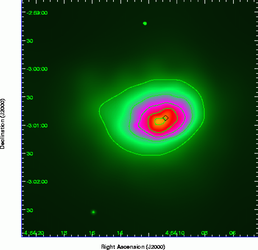
An adaptively smoothed image of the diffuse emission of this cluster was created by using CIAO’s dmfilth to replace point sources detected by wavdetect with a Poisson distribution based on the sky background local to the sources. The resulting diffuse image was smoothed to a minimum significance level of $3\sigma$; the $1\times 1$ binned exposure map described above was smoothed using the same scales as derived for the emission image, then it was divided from the smoothed image (Figure 2).

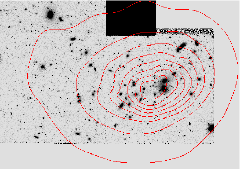
We compared the locations of X-ray features to those in the optical by constructing a Hubble Space Telescope (HST) I-band image of the cluster (Figure 3). We drizzled together HST WFPC2 I-band (F702W) observations consisting of 4 independent exposures with a total exposure time of 10,400 seconds. The HST image required a correction to the World Coordinate System keywords in the header based on the location of GSC2.2 objects in the field. The shift was -0.23 seconds in RA and +1.5 arcseconds in declination.

We note that the nominal center of the X-ray isophotal contours is not located on the brightest cluster galaxy (BCG), identified by a diamond on Figure 2. The large galaxy to the south of the BCG is a foreground galaxy (John Stocke, private communication). The isophotes near the BCG seem to be distorted, perhaps suggesting that the BCG or a system centered on the BCG may be contributing to the surface brightness there. The elliptical BCG is at 04h 54m 10.8s, $-03\arcdeg~{}00\arcmin~{}52.4\arcsec$ ($x=4164$, $y=3856$ in the physical coordinates of the original Chandra image).

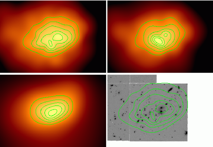
We did not detect any evidence for statistical temperature variations in our spectral data. However, a qualitative assessment of possible temperature or absorption variations across the cluster can be made from the inspection of color maps. We divided the events data into three energy bands: 0.2–1.5 keV, 1.5–4.5 keV, and 4.5–7.0 keV. We created monoenergetic exposure maps for the mode of the photons’ energies in each band, corresponding to 0.9, 1.6, and 4.6 keV respectively. We then adaptively smoothed each image, omitting the brightest point source [#6 from Molnar et al. 2002]; the identical scales were used to smooth each exposure map. After dividing the data by the exposure map (setting pixel values with exposure time less than 1.5% the total time to 0.0), we then created contour maps (Figure 4).

The main conclusion from Figure 4 is that the emission peaks shift with bandpass; in addition, the centroid of the emission shifts with bandpass. The positions of the peaks were identified on the maps. We also computed centroid positions based on the unsmoothed data, weighted by the exposure maps, inside a region $256\arcsec\times 256\arcsec$. In the soft bandpass, the highest peak lies on the BCG, with a secondary peak to the east-south-east. The centroid is somewhat west of the primary peak, near 4h 54m 11.26s, $-03\arcdeg\,00\arcmin\,56\arcsec$. In the mid-energy bandpass, the brightest peak is closer to the soft bandpass secondary peak, and a fainter peak is associated with the BCG. The centroid is near 4h 54m 11.32s, $-03\arcdeg\,00\arcmin\,56\arcsec$, $6\arcsec$ west of the centroid in the soft band. In the hardest energy, there is no obvious peak near the BCG, and the centroid of this single-peaked distribution is close to the position of the primary peak in the mid-energy bandpass. The hard peak 4h 54m 11.48s, $-03\arcdeg\,00\arcmin\,55\arcsec$. The soft X-ray emission near the BCG is nearly circular, embedded in a large-scale elliptical emission closer to that of the global cluster. The mid-energy peak has a position angle of $65-70\arcdeg$ E of N that is significantly different from the globally-fit (see the next section) position angle of $100\arcdeg$ E of N. The global position angle of the 0.7–7.0 keV data is closer to the position angle of the hardest emission, which is smooth, and the position angle of the $>30\arcsec$ contours of the softest emission. In summary, there seems to be two peaks to the emission, with a soft peak that lies on the BCG and a harder peak that is offset from the BCG.

3.3 X-ray Surface Brightness Models

3.3.1 Beta-Model Fits

We fit the X-ray suface brightness data to spherical and elliptical $\beta$-models, using SHERPA, the model-fitting engine of CIAO. The central portion of a 0.7-7.0 keV image was binned by a factor of 8 (1 original pixel $=0\farcs 4920$), then an exposure map of the same size was binned to the same resolution. The reprojected background map was filtered and binned identically. We found little advantage to using the background map in this case - results were similar with and without the background map for the fits without exposure corrections. Since CIAO 2.3 does not simultaneous allow for the use of exposure maps and external background, we report fits without the background maps. In the following section, we report fits with and without the exposure correction in order to demonstrate the effect of the exposure correction. Background counts were not subtracted but fit as a constant flat contribution to the total signal. Even binned, the total counts inside each binned pixel was not high, so we experimented with the use of various statistics: the low-count modification to $\chi^{2}$ by Gehrels (1986), the iterative $\chi^{2}$ method from Kearns, Primini, & Alexander (1995), and Cash maximum likelihood statistics (Cash 1979). We found that the Gehrels (1986) statistics could result in unusual and unstable results which were very sensitive to the region being fit, while the Cash (1979) statistics and the “Primini” $\chi^{2}$ method (Kearns et al. 1995) produced similar results to each other and consistent uncertainties. We therefore use a simplex method with Cash statistics for our results. The fit was limited to the central $100\arcsec$ of the cluster. We note that this radius, as we shall see, is about two or three times the core radius and is approximately equivalent to $r_{2000}$, inside which the mean mass density exceeds the critical density at $z=0.538$ by a factor of 2000. This radius is contained in the range of $r_{2500}-r_{200}$, within which the measured gas fraction is expected to be close to that of the cluster as a whole (Evrard, Metzler, & Navarro 1996).

We report the results of fits to a spherical $\beta-$model with $S_{X}=S_{X0}[1+(r/r_{core})^{2}]^{-3\beta+1/2}$ and $r=\sqrt{(x-x_{0})^{2}+(y-y_{0})^{2}}$ and to an elliptical $\beta-$model (Equation 1) in Table 6.

$$S_{X}(x,y) = S_{X}(r)=S_{X0}(1+(r/r_{core})^{2})^{-3\beta+1/2}$$ (1)

$$r(x,y) = \frac{\sqrt{x^{2}_{n}(1-\epsilon)^{2}+y^{2}_{n}}}{1-\epsilon}$$

$$x_{n} = (x-x_{0})\cos\theta+(y-y_{0})\sin\theta$$

$$y_{n} = (y-y_{0})\cos\theta+(x-x_{0})\sin\theta$$

The fit parameters include core radius $r_{core}$, $\beta$, cluster central position $x_{0}$ and $y_{0}$, ellipticity $\epsilon$, position angle $\theta$, and amplitude $S_{X0}$. We report best-fit parameters to 90% projected confidence for a single interesting parameter, (or $\Delta\chi^{2}=2.7$; $1.6\sigma$), where all other parameters are allowed to take on their best fit values.

The best-fit spherical model results in $r_{core}=31\arcsec\pm 3.5\arcsec$, $\beta=0.70\pm 0.07$ (the uncertainties of $r_{core}$ and $\beta$ are correlated), and a central amplitude of $S_{X0}=(1.55\pm 0.06)\times 10^{-7}$ in units of photons s^-1 cm^-2 arcsec^-2 ($0.7-7.0$ keV). If the data were not exposure-corrected, we obtained somewhat different best-fit parameters for the shape of the spherical $\beta-$model: $\beta=0.67\pm 0.07$, $r_{core}=28\arcsec\pm 3.3\arcsec$. The fit parameters did not change within the statistical uncertainties with the use of the exposure map.

If we allow the ellipticity and the position angle of an elliptical $\beta-$model to be free, the best-fit $r_{core}$ is $40.2\arcsec\pm 4.1\arcsec$ along the semi-major axis and $\beta$ is $0.79\pm 0.08$ (Figure 5). The cluster emission is elliptical, with an ellipticity $\epsilon_{SHERPA}=0.271\pm 0.016$, and a position angle of $\theta=0.17\pm 0.03$ radians S of E or $100\pm 2$ degrees E of N, aligned almost directly East-West. The amplitude, in units of photons s^-1 cm^-2 arcsec^-2, is $(1.52\pm 0.06)\times 10^{-7}$ ($0.7-7.0$ keV) The background is $(2.09\pm 0.65)\times 10^{-9}$ ($0.7-7.0$ keV). We also report the best-fit to data without an exposure correction in Table 6. We note that the exposure-corrected data fit to an elliptical model had the most symmetric uncertainties in the background level.

When the region around the BCG was excluded from the fit, the results did not change, except for the larger error bars on $r_{core}$ and $\beta$. Therefore, a large fraction of the emission from the cluster can be modelled robustly by an ellipsoidal $\beta-$model.

The center of a 2-D $\beta-$model fit to the 0.7-7.0 keV data was independent of whether an elliptical or a spherical model was fit: 04h 54m 10.9s, $-03\arcdeg\,00\arcmin\,47\farcs 1$. Relative to the surface brightness data contours, the center of the best fit lies between the BCG elliptical and the centroid of the bulk of the X-ray emission. This location is about $7.5\arcsec$ west of the BCG, whose position is defined in our corrected HST data.

The brightness of a point source that could hide in any $8\times 8$ ($4\arcsec\times 4\arcsec$) bin depends on the number of counts in each bin. The brightest point source that could hide in these data would be, conservatively, a $5\sigma$ source in the center of the cluster. Such a source would need have to have about 61 total counts, or $>1.5\times 10^{-3}$ counts s^-1 (0.7-7.0 keV), or $F_{x}\sim 1.1\times 10^{-14}\mbox{erg~{}s${}^{-1}$~{}cm${}^{-2}$}$ in the same bandpass to be detected above the cluster. A $3\sigma$ source in the highest flux bins would have to have 33 total counts, or $F_{x}\sim 6\times 10^{-15}\mbox{erg~{}s${}^{-1}$~{}cm${}^{-2}$}$ (0.7-7.0 keV). The largest positive excess over an elliptical beta-model in our data is $<2.8\sigma$. If the data are binned to a finer grid of $4\times 4$ pixels, the maximum hidden point source flux is reduced to approximately $2/3$ the fluxes of the $8\times 8$ pixel regions.

3.3.2 Goodness of Fits

We examined maps of the residuals between the best-fit models and the $8\times 8$ binned data. The number of bins where the spherical model residuals which are greater than $2\sigma$ from the model is 49, whereas the corresponding number of bins for the elliptical model residuals is 23. No bins exhibit a departure of greater than $\sim 3\sigma$ from the model. The most prominent features in the maps of residuals align with a linear feature with a depth of about 20% of the total in the exposure map. The alignment suggests that at least some of the residuals are related to an imperfect exposure correction.

If we bin the data and the simulations produced from the best-fit models into radial profiles, then compute a $\chi^{2}$, the resulting fits are both rejected. The spherical $\beta-$model results in a $\chi^{2}=162.5$ for 22 degrees of freedom. By adding two additional parameters with the elliptical $\beta-$model, we obtain a $\chi^{2}=116.8$ for 20 degrees of freedom. This improvement is statistically significant, but the fit is still formally rejected. Figure 6 shows the radial plot, with 27 points for the data in a histogram. The elliptical model is plotted with a solid line and the spherical $\beta-$model is plotted with a dashed line. The residuals are plotted below the radial surface brightness plot. The spherical model shows higher residuals at $r\sim 40-80\arcsec$.

In summary, the data clearly exclude a traditional spherical $\beta-$model. An elliptical beta model better represents the surface brightness distribution, both in a statistical and in a qualitative sense, but it too is an incomplete description of the data. The 2D binned data do not show any statistically significant departures from the model, mainly because of the limitations of bins with small numbers of counts in them; in contrast, radially binned data seem to exclude the models. We are left, then, to use the $\beta-$model approximation to derive gas masses and isothermal gravitational masses, but to retain the caveat that we are, as yet, limited by an incomplete description of the data.

4 Masses and Mass Profiles

Many workers in this field have simply approximated the surface brightness profiles of clusters where deprojection is not possible by extracting radial profiles. These radial profiles are generally fit to beta-model functional forms. We take an additional step (see also Hughes & Birkinshaw 1998) to previous studies in the next sections. In addition to reporting the results for MS0451.6-0302 from a spherically symmetric analysis, we also estimate the impact of a first-order correction to the spherically symmetric case by applying the results of an elliptical beta-model fit to the derivation of the gas mass and other cluster properties. We find that the derived gas mass and gas fraction are affected somewhat by moving from the spherically symmetric to the ellipsoidal case. In contrast, as other workers have also found in a study of ROSAT clusters (Piffaretti, Jetzer, & Schindler 2002), the gravitational mass enclosed inside a sphere is not significantly affected by the spheroidal assumption.

In the following section, we describe the formalism we use to derive the gas mass profile for an isothermal spherical and ellipsoidal beta-model for the gas distribution, including, for completeness, a discussion of the Sunyaev-Zel’dovich temperature decrement.

4.1 Spherical Model

For a spherical isothermal $\beta-$model, the electron number density $n_{e}$ follows the model

$$n_{e}(\theta)=n_{e0}\left(1+\frac{\theta^{2}}{\theta_{c}^{2}}\right)^{-3\beta/2},$$ (2)

where n_e0 is the central electron density. The central electron density can be derived from

$$n_{e0}=\sqrt{\frac{S_{X0}}{A_{1}D_{A}}}$$ (3)

where $S_{X0}$ is defined in units of counts s^-1 sr^-1, $D_{A}$ is the cluster angular distance in units distance per radian and $A_{1}$ is defined below.

The X-ray surface brightness, $S_{X}$, in terms of the angular distance diameter, $D_{A}$, is

$$S_{X}(\theta)={\frac{1}{4\pi(1+z)^{3}}}\int{D_{A}n_{e}^{2}\Lambda_{e}d\zeta}=S_{Xo}\left(1+\frac{\theta^{2}}{\theta_{c}^{2}}\right)^{1/2-3\beta},$$ (4)

where $S_{X0}$ is the central X-ray surface brightness, $z$ is the cluster redshift, and $\Lambda_{e}$ is the X-ray cooling function of the ICM in the cluster rest frame. $\Lambda_{e}=\epsilon/n_{e}^{2}$, where $\epsilon$ is the spectral emissivity (Birkinshaw, Hughes, & Arnaud 1991; Hughes & Birkinshaw 1998).

The Sunyaev Zel’dovich Effect, SZE, is the change in the observed brightness temperature of the Cosmic Microwave Background (CMB) radiation resulting from passage of the CMB radiation through the ionized gas permeating a galaxy cluster (Sunyaev & Zel’dovich 1972; Sunyaev & Zel’dovich 1980). The temperature decrement can be described by a spherical isothermal $\beta$ model if the density of the cluster follows the form $[1+(r/r_{core})^{2}]^{-3\beta/2}$. (Cavaliere & Fusco-Femiano 1976; Birkinshaw 1999). The resulting temperature decrement is given by

$$\Delta T=f(x)T_{CMB}D_{A}\frac{\sigma_{T}k_{B}}{m_{e}c^{2}}\int{n_{e}T_{e}d\zeta}=\Delta T_{0}[1+\frac{\theta^{2}}{\theta_{c}^{2}}]^{1/2-3\beta/2},$$ (5)

where $f(x)$ is the frequency dependence of the SZE, $T_{CMB}$ is the temperature of the CMB radiation, $\sigma_{T}$ is the Thomson cross section, $k_{B}$ is the Boltzmann constant, $m_{e}$ is the electron mass, $n_{e}$ is the electron density, $T_{e}$ is the cluster temperature, $\Delta T_{o}$ is the central temperature decrement, $\theta$ is the angular radius in the plane of the sky, $\theta_{c}$ is the angular core radius, and $\beta$ is a shape parameter that describes the radial falloff of the gas distribution from the beta-model. The integration is along the line of sight $\ell$ = D_A$\zeta$ (Hughes & Birkinshaw 1998; Carlstrom et al. 2000).

In principle, the cluster distance, D_A, can be estimated independently of $H_{0}$ by combining X-ray observations with Sunyaev Zel’dovich observations. Solving equations (3, 5, 6) for the angular diameter distance, $D_{A}$, in terms of known parameters (Myers et al. 1997; Hughes & Birkinshaw 1998; Birkinshaw 1999; Patel et al. 2000; Reese et al. 2002), gives

$$D_{A}=\Bigl{(}\frac{\Delta T_{0}}{A_{2}}\Bigr{)}^{2}\frac{A_{1}}{S_{Xo}},$$ (6)

where

$$A_{1}=\frac{1}{4\pi(1+z)^{3}}\frac{\epsilon_{o}}{n_{eo}^{2}}\sqrt{\pi}\frac{\Gamma(3\beta-1/2)}{\Gamma(3\beta)}\theta_{c},$$ (7)

$$A_{2}=\delta_{SZE}(x,T_{e})T_{CMB}\frac{k_{B}T_{e}}{m_{e}c^{2}}\sqrt{\pi}\frac{\Gamma(3\beta/2-1/2)}{\Gamma(3\beta/2)}\theta_{c}.$$ (8)

where $\delta_{SZE}=-1.879$ is the relativistic correction to the frequency dependence for $kT=10.8$ keV (Itoh, Kohyama & Nozawa 1998).

The gas mass derived from the assumption of a $\beta-$model and spherical symmetry is simply

$$M_{gas}(<r)=4\pi\mu m_{H}n_{e0}\int^{r}_{0}[1.0+(r/r_{core})^{2}]^{-3\beta/2}r^{2}dr.$$ (9)

The corresponding gravitating mass (Evrard et al. 1996), from the assumptions of hydrostatic equilibrium ($\nabla P=\rho_{g}\nabla\phi$ and $\nabla^{2}\phi=-4\pi G\rho_{M}$) and isothermality ($\rho=-\frac{kT}{4\pi G\mu_{h}m_{h}}\nabla^{2}\ln{\rho_{g}}$), is

$$M(<r)=\frac{3\beta kTr}{G\mu_{H}m_{H}}\left(\frac{r}{r_{core}}\right)^{2}\left/\left[1+\left(\frac{r}{r_{core}}\right)^{2}\right]\right.$$ (10)

where $\beta$ and $r_{core}$ are from the fit to a spherical $\beta-$model, $kT$ the X-ray temperature, $G$ the gravitational constant, $\mu_{H}$ the mean mass per particle ($\mu_{H}=0.59$), and $m_{H}$ the mass of a proton. Note that for large $r$, an isothermal mass distribution diverges like $r$.

A somewhat more physical assumption may be that the temperature is not constant (at least outside the radius where we have direct measurements). We can allow for an unobserved temperature gradient by approximating the system with a “polytropic” equation of state (Lea 1975) where

$$P=K_{\rm eff}\rho_{g}^{\gamma_{\rm eff}}$$ (11)

and

$$T=\frac{P}{\rho}\mu_{H}m_{H}=K_{\rm eff}\mu_{H}m_{H}\rho_{g}^{\gamma_{\rm eff}-1}$$ (12)

In the spherical case where the gas is distributed like the beta-model,

$$M(<r)=\frac{3\beta\gamma kT(0)r}{G\mu_{H}m_{H}}\left(\frac{r}{r_{core}}\right)^{2}\left/\left[1+\left(\frac{r}{r_{core}}\right)^{2}\right]^{b}\right.$$ (13)

where $\gamma$ is the effective polytropic index, $K_{\rm eff}$ is the effective polytropic constant $K$, $kT(0)$ is the X-ray temperature at radius $r=0$, and $b=1.5\beta(\gamma-1)+1$ (See also Henriksen & Mushotzky 1986). Nonphysical masses result if $\gamma>1+1./3\beta$ (or $\gamma>1.41$ for $\beta=0.8$). Typical polytropic indices found for nearby relaxed clusters are around $1.1-1.2$ (e.g. De Grandi & Molendi 2002; Markevitch et al. 1999). The ratio of the polytropic mass to an isothermal mass is $\gamma[1+(r/r_{c})^{2}]^{-1.5\beta(\gamma-1)}$. If MS0451 has an effective polytropic index of $\gamma=1.2$ and surface brightness index $\beta=0.8$, then the enclosed gravitational mass at 5 core radii would be about a factor of $0.54$ that of the isothermal mass. If $\gamma=1.1$, the factor is $0.74$. The mass at $r_{500}$ is thus rather sensitive to $\gamma$.

4.2 Ellipsoidal Model

If we relax the assumption that the cluster electron density distribution is spherically symmetric and assume that the distribution is a prolate or oblate spheroid, we can derive equivalent expressions for $n_{e0}$ and $D_{A}$. Here, we assume that the gas follows an ellipsoidal beta-model distribution as follows:

$$\rho_{g}=\rho_{o}[1+\frac{\sum_{i=1}^{3}e_{i}^{2}x_{i}^{2}}{r_{c}^{2}}]^{-3\beta/2},$$ (14)

where $\rho$ is the gas density, $x_{i}$ the intrinsic coordinate distances in each of three dimensions, $r_{c}$ the core radius in the direction of the semi-major axis, and $e_{i}$ the ratio of the major to minor axes in each direction. For a prolate model of intrinsic eccentricty $e$, where the axis of symmetry is the 3rd coordinate, $e_{i}=[e,e,1.0]$ and for an oblate model, $e_{i}=[1,1,e]$.

We follow the derivations from Hughes & Birkinshaw (1998; HB98) and Fabricant, Rybicki, & Gorenstein (1984), but present them here in order to use terminology similar to the previous section. The expressions for $D_{A}$ and $n_{e0}$ are identical. The expressions $A_{1}$ and $A_{2}$ can be modified for an oblate distribution where $i$ is the angle of the axis of symmetry with respect to the line of sight ($i=90\arcdeg$ corresponds to the axis of symmetry lying in the plane of the sky):

$$A_{1,oblate}=A_{1}\frac{\sqrt{1-e_{HB}^{2}\cos{i}^{2}}}{\sin{i}}$$ (15)

$$A_{2,oblate}=A_{2}\frac{\sqrt{1-e_{HB}^{2}\cos{i}^{2}}}{\sin{i}}$$ (16)

and a prolate distribution gives:

$$A_{1,prolate}=A_{1}\frac{\sqrt{e_{HB}^{2}-\cos{i}^{2}}}{e_{HB}^{2}\sin{i}}$$ (17)

$$A_{2,prolate}=A_{2}\frac{\sqrt{e_{HB}^{2}-\cos{i}^{2}}}{e_{HB}^{2}\sin{i}}$$ (18)

where $e_{HB}$ is the observed semi-major/semi-minor axis ratio. The eccentricity $\epsilon$ from the SHERPA elliptical $\beta-$model is related to $e_{HB}$ by $e_{HB}=1.0/(1.0-\epsilon)$. The intrinsic axis ratio $R$ from Fabricant et al. (1984) can be recovered from the expression $e_{int}=Re_{HB}$ where $R_{oblate}=\frac{\sqrt{1-e_{HB}^{2}\cos{i}^{2}}}{\sin{i}}$ and $R_{prolate}=\frac{\sqrt{e_{HB}^{2}-\cos{i}^{2}}}{e_{HB}\sin{i}}$.

The intrinsic coordinate is related to the observed coordinate by the usual rotation transformation where the rotation is around the first axis:

$$x_{1,i}=x_{1,o}$$ (19)

$$x_{2,i}=x_{3,o}\sin{i}+x_{2,o}\cos{i}$$ (20)

$$x_{3,i}=x_{3,o}\sin{i}-x_{2,o}\cos{i}$$ (21)

We note that the expressions for $A_{1}$ and $A_{2}$ diverge for certain values of the inclination angle $i$. At $i=0$, a prolate and oblate distributions would appear as perfectly circular clusters to the observer, and no information could be recovered regarding the elongation along the line of sight. Also, for $i\leq\arccos(1.0/e_{HB})$, an oblate distribution cannot reproduce the observed axis ratio $e_{HB}$. Therefore, for an oblate distribution to be plausible, there is a minimum inclination angle $i$.

The gravitating mass density $\rho_{M}$ can be computed directly from the X-ray temperature and gas distribution, using the assumptions of hydrostatic equilibrium and isothermality as above. The gas distribution can be recast as:

$$\rho_{g}=\mu_{e}m_{h}n_{e0}u^{-3\beta/2}$$ (22)

where $u=[1+\Sigma_{i=1}^{3}\frac{e_{i}^{2}x_{i}^{2}}{r_{c}^{2}}]$ and $\mu_{e}=1.4/1.2$. Here $r_{c}$ is the core radius along the longest axis, and, for convention, the axis of symmetry is along the $z$ or $3$ axis and $e_{i}$ is the axis ratio. So for the general case where

$$\rho_{M}=-\frac{kT}{\mu_{H}m_{H}G4\pi}\nabla^{2}\ln\rho_{g}$$ (23)

the result can be written analytically where

$$\rho_{M}=-\frac{3\beta kT}{\mu_{H}m_{H}G4\pi r_{c}^{2}u^{2}}\left[-\Sigma_{i=1}^{3}\left(\frac{2e_{i}^{2}x_{i}}{r_{c}}\right)^{2}+u\Sigma_{i=1}^{3}{2e_{i}^{2}}\right].$$ (24)

For the case $e=[1,\,1,\,1]$, Equation 24 reduces to the spherical case.

This derivation assumes that the dark matter is distributed in concentric, similar ellipsoids. The isothermal ellipsoidal $\beta-$model derived here is not physically realistic over all scales, since large eccentricities can result in negative, unphysical dark matter densities. For small eccentricities, this derivation is a perturbation of the spherical $\beta-$model, and is not a bad approximation to the effects of moderate elongation. However, we warn that this derivation is only intended to explore the implications of an ellipsoidal model.

5 Cluster Luminosity

We derive the cluster luminosity inside a radius of $1h^{-1}$ Mpc. The total count rates (0.7-7.0 keV) are derived by integrating the best fit elliptical $\beta-$model inside a circle of $244\arcsec$ (flat, $\Omega_{M}=0.3$ cosmology). The aperture correction from $r=85\arcsec$ is 1.074, for 0.319 counts s^-1 total. From the spectral fits with XSPEC, we have derived the conversion from count rate to luminosity and flux for the best-fit Raymond-Smith model with $kT=10.6$ keV. Our results here are not too sensitive to the details of the spectral fit. We report the observed fluxes and the intrinsic luminosities in Table 7.

If the luminosity-temperature ($L_{x}-T_{x}$) relation does not evolve, the predicted temperature for this cluster from the Markevitch (1998) L-T relation is $10.5-12.2$ keV, depending on whether we use the ROSAT band relation or the bolometric relation in Markevitch (1998). Therefore the temperature and luminosity we measure for this cluster at $z=0.538$ is consistent with the local luminosity temperature relation.

6 Central Density, Gas Mass, and Total Mass from X-ray Properties

The estimates for X-ray properties based on the X-ray data alone are reported in Table 8. Here we use the results of the $\beta-$model fits and the X-ray properties alone to derive the cluster gas mass and the baryonic fraction, assuming isothermality, and hydrostatic equilibrium as described in the previous section. We assume a temperature of $kT=10.6$ keV (this work), along with an emissivity of $1.343\times 10^{-12}\,n_{e}^{2}\,{\rm count\,s}^{-1}\,{\rm cm}^{5}$. For the spherical $\beta-$model, here we assume a core radius $31\arcsec$, $\beta=0.75$, central surface brightness of $0.34$ counts arcmin^-2 s^-1, $z=0.5386$. We derive a central electron density of $n_{e0}=(0.0146\pm 0.002)h^{1/2}$ cm^-3 using Equation 3. For elliptical $\beta-$models we use the best-fit parameters from Table 6. The $r_{500}$ radius, inside which the mean density is 500 times that of the critical density at that redshift $z$ ($\rho_{c}(z)=\rho_{c}(0)(\Omega_{M}(1+z)^{3}+\Omega_{\Lambda})$ if $\Omega_{M}+\Omega_{\Lambda}=1$) for this cluster is $0.97\pm 0.13h^{-1}$ Mpc for $M_{500}=(8.6\pm 1.2)\times 10^{14}h^{-1}M_{\odot}$. For an ellipsoidal modal, $M_{500}=(9.1\pm 1.2)\times 10^{14}h^{-1}M_{\odot}$. The uncertainties include the uncertainty in the statistics of the spectral and spatial fitting, added in quadrature, but not the systematic uncertainty in the spectral fit.

The gas mass inside $r_{500}$ is $(5.6\pm 3.3)\times 10^{13}h^{-5/2}M_{\odot}$ for these fit parameters, corresponding to a baryonic fraction in hot gas of $0.065\pm 0.01h^{-3/2}$. The uncertainties here include systematic and statistical uncertainties added in quadrature (Patel et al. 2000). However, we will show that the uncertainties in the shape and orientation of the cluster lead to even larger uncertainties ($\sim 0.03$) in the gas fraction. If we could constrain the shape and orientation of a given cluster, one of the largest systematic uncertainties would be reduced and we could refine the estimates of the gas fraction. Here we will show that while current data are not quite good enough to accomplish this goal, there is promise in the technique for data in the near future. The estimates for masses, electron density, and gas fraction are reported in Table 8.

As pointed out first by Briel, Henry, & Böhringer (1992) (and subsequently expanded upon by White et al. 1993 and others), the gaseous baryonic fraction in clusters can be used to place a limit on $\Omega_{m}$, given a constraint on the baryonic density $\Omega_{B}$ from primordial nucleosynthesis and deuterium measurements. If we use $\Omega_{B}=0.019\pm 0.002h^{-2}$ from Burles & Tytler (1998), we obtain an upper limit to $\Omega_{M}$ of $0.29\pm 0.05h^{1/2}$.

To get a better census of the baryons in this cluster, we can also account for the baryons associated with the galaxies, which in general are only a small contribution to the total amount of baryons in clusters. The amount of mass associated with the galaxies from the total optical luminosity of the cluster was estimated by assuming a mass to light ratio for the galaxies. Carlberg et al. (1996) measure a k-corrected r-band (Gunn) luminosity inside their definition for $r_{200}=r_{v}=1.4\pm 0.17h^{-1}$ Mpc of $4.5\times 10^{12}h^{-2}L_{\odot}$. For their assumed cosmology of $q_{0}=0.1$, $r_{v}$ is $346\arcsec$. Scaling to the same projected radius as our assumed $r_{500}=0.95h^{-1}$ Mpc, or $214\arcsec$, $L_{500,R}=8.7\times 10^{11}h^{-2}L_{\odot}$, assuming $L(<\theta)\propto\theta$. The average elliptical galaxy $M/L_{R}=6.64h$ (van der Marel 1991) for Johnson R. The conversion from Gunn r to Johnson R is about a factor of 1.8 for elliptical galaxies (Frei & Gunn 1994), including a color term for $g-r\sim 0.75$ (Carlberg et al. 1996). Therefore the mass associated with the galaxies alone could be as high as $1\times 10^{13}h^{-1}\mbox{M${}_{\odot}$}$ inside a projected angular distance of $214\arcsec$. (We did not take into account a weak dependence of $M/L$ on the luminosity of the individual galaxy (van der Marel 1991).) The corresponding $M_{gal}/M_{gas}\approx 0.15h^{3/2}$, or $0.10$ if $h=0.75$. If most of the matter in this $M/L$ ratio is baryonic, the gas fraction of the cluster can now be corrected to a baryon fraction. The estimate for $\Omega_{M}$ that would be consistent with primordial nucleosynthesis and deuterium constraints becomes $\Omega_{M}=0.29h^{1/2}[1+0.15h^{3/2}]^{-1}$ or, for $h=0.75$, $\Omega_{M}=0.23(\pm 0.05)$. The estimated value of $\Omega_{M}$ increases somewhat if some of the matter ascribed to elliptical galaxies here is not baryonic.

We can turn this calculation around, if we use WMAP values for $\Omega_{M}$, to calculate what fraction of the baryons are in the ICM. The WMAP ratio of baryons to total matter is independent of $H_{0}$, $\Omega_{B}/\Omega_{M}=0.166$. The gas fraction estimated for this cluster, for $H_{0}=71$, is approximately 0.10; we will show later that this value could be as high as 0.12-0.14, depending on geometric assumptions. Therefore, at least 60% $h_{71}^{-3/2}$ of the baryons in the cluster are in the hot ICM. Unless cluster-specific processes like ram-pressure stripping are particularly effective and efficient at removing baryons from the galaxies, one hypothesis based on this observation is that most of the baryons in the universe may lie between the galaxies. Studies of the Lyman-alpha forest suggest that is the case at high redshift, $z\sim 3$ (Fukugita, Hogan & Peebles 1998; Hui et al. 2002). Assessment of gas fractions in clusters suggest it is also true at lower redshifts; refinements of such measurements could show the dependence on mass scale of the efficiency of galaxy formation (David et al. 1990; Bryan 2000).

6.1 Comparison to Other Mass Determinations

We compute a gravitational mass inside $r_{500}$ of $M_{500}=(8.6-8.9)\times 10^{14}h^{-1}\mbox{M${}_{\odot}$}$ or, alternatively, $M(r<1~{}h^{-1}$ Mpc$)=(8.8-9.2)\times 10^{14}h^{-1}\mbox{M${}_{\odot}$}$. In this section, we compare this mass estimate to other mass estimates for this cluster, from the literature. One challenge in the literature is to compare masses estimated at radii defined in many different ways with several cosmological assumptions and definitions built in. As an aside, we would like to encourage observers to report enclosed masses at either a metric radius or a fixed angular radius, in addition to $M_{200}$ or $M_{500}$ if desired, in order to minimize the computations required to make direct comparisons.

The gravitational mass from optical, the virial mass, can be derived from the one-dimensional velocity dispersion $\sigma_{v}=1371\pm 105$ km s^-1 and the estimated virial radius $R_{v}=1.4h^{-1}$ Mpc (Carlberg et al. 1996). See Carlberg et al. (1996) for details on how the virial radius was computed, based on CNOC observations for MS0451.6-0302 (Ellingson et al. 1998). For this cluster, Carlberg et al. (1996) obtain an $M_{200}=1.8\times 10^{15}h^{-1}\mbox{M${}_{\odot}$}$, for an open $\Omega_{m}=0.2$ cosmology. Adjusting to our flat $\Omega_{m}=0.3$ cosmology and extrapolating to $r_{500}$ by assuming that $\rho\propto r^{-2}$, we obtain $M_{500}=(1.4\pm 0.25)\times 10^{15}h^{-1}\mbox{M${}_{\odot}$}$. The optical $r_{500}$ is larger than the $r_{500}$ estimated from the X-ray temperature and surface brightness distribution. The optically-derived mass at the same angular scale as our X-ray estimate (also taking into account the differences in the angular distance scale between the two cosmologies) of $0.97h^{-1}$ Mpc, is $(1.3\pm 0.25)\times 10^{15}\mbox{M${}_{\odot}$}$. The total mass ($M_{500}$) calculated from the X-ray values ($(8.6-9.1)\pm 1.2\times 10^{14}\mbox{M${}_{\odot}$}$) is only somewhat less than that derived from the optical velocity dispersion and the positions of the member galaxies by Carlberg et al. (1996). Within the uncertainties of both estimates, however, they are consistent, especially if the underlying dark matter potential is somewhat elongated, which gives the higher X-ray mass estimate. We will discuss this dependency further in the next section.

Clowe et al. (2000) find a best-fit mass for MS0451.6-0302, corrected for projection, to their ground-based weak-lensing data (obtained with the Keck telescope) with a NFW (Navarro, Frenk, & White 1996) dark matter profile where the concentration index $c=1.5$ and $r_{200}=1060h^{-1}$ kpc, assuming an underlying cosmology of $\Omega_{M}=1$ and $z=0.55$. We recomputed the NFW parameters for the same weak lensing data, assuming a flat cosmology with $\Omega_{M}=0.3$ and a cluster redshift $z=0.5386$, for a best-fit of $c=1.82$ and $r_{200}=1474h^{-1}$ kpc. We also fit the 1D velocity dispersion of $\sigma=986^{+53}_{-58}$ km s^-1 (uncertainties are $1\sigma$) assuming an isothermal mass distribution. As in Clowe et al. (2000), the concentration is not constrained very well because of the small field of view for the Keck data. The constraints on $r_{200}$ and $c$ with the revised cosmology are plotted in Figure 7. The $1\sigma$ minimum for the value of $r_{200}$ is $1100h^{-1}$ kpc. The mass could be much higher for lower concentrations $c$. However, typical concentrations of simulated clusters are usually higher than $\sim 3-5$ (Eke, Navarro, & Frenk 1998; Brainerd, Goldberg, & Villumsen 1998). So the lower mass estimates are more likely, based on theoretical expectations of the minimum concentrations.

There are three main sources of systematic error in the estimation of weak lensing masses. The uncertainty about the actual redshifts of the background galaxies induces an uncertainty of 15-20% in the mass for clusters at $z\sim 0.5$. In addition, the Clowe et al. (2000) magnitude and color selection criteria for removing the red sequence and bright foreground galaxies did not remove the blue dwarf cluster members. Those members dilute the shear signal by an estimated 10-20%, increasing the mass estimate by the same amount. Also, if the dwarfs are concentrated in the core like the giant ellipticals, this effect lowers the measured concentration $c$ as well.

The best-fit weak lensing mass inside of $r_{500}$, therefore, is $M_{500}=8.4\times 10^{14}h^{-1}\mbox{M${}_{\odot}$}$, with a $1\sigma$ minimum mass of $M_{500}>3.5\times 10^{14}h^{-1}\mbox{M${}_{\odot}$}$. The weak lensing mass increases by $10-20\%$ if the estimated effect of dilution is taken into account. Even so, the weak lensing mass is consistent with the mass derived from the velocity dispersion and the mass derived from the X-ray data.

The third systematic in the mass conversion comes from the assumption of a cluster shape when converting from a projected mass to the mass inside a sphere. The weak lensing signal reports the mass in a cylinder along the line of sight, which is converted into a mass within a spherical volume in the analysis process. (The masses we discuss above are masses inside a sphere.) X-ray temperatures are affected by the mass inside a sphere. The full comparison of an X-ray-determined mass with a weak lensing mass requires the knowledge of the cluster’s intrinsic shape and mass distribution. In the next section, we will use the SZE data to constrain the intrinsic inclination and ellipticity of this decidedly elliptical cluster, and in the following section, we explore how the assumption of an ellipsoidal cluster affects our conclusions.

7 Sunyaev-Zel’dovich Effect and Three Dimensional Shape

We present here a joint analysis of the Sunyaev Zel’dovich Effect observations, the Chandra surface brightness map, and the Chandra spectral fits for MS0451.6-0302.

7.1 Sunyaev-Zel’dovich Observations

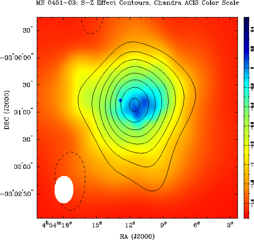
The SZE observations (Figure 8) for MS0451.6-0302 were taken at the Owens Valley Radio Observatory, OVRO, in 1996 for a total of 30 hours using two 1 GHz channels centered at 28.5 GHz and 30.0 GHz as reported by Reese et al. (2000). One point source was found in the cluster field and is located at 04h 54m 22s, $-03\arcdeg\,01\arcmin 26\arcsec$ (J2000).

7.2 Joint X-ray and SZE Modeling

The spatial parameters of the intra-cluster medium (ICM) were constrained by jointly fitting the Chandra X-ray spatial data, and the interferometric OVRO SZE data to a composite spherical $\beta-$model using the Jointfit analysis package developed by Reese et al. (2000). The fitting algorithm simultaneously fits the source and background X-ray models and the SZE interferometric models using a downhill simplex method that maximizes the likelihood function (Cash 1979; Kendall & Stuart 1979; Hughes & Birkinshaw 1998). We used Jointfit rather than SHERPA here to include the SZE data. We are encouraged that the results from both fitting packages, using different statistical assumptions, result in similar X-ray surface brightness parameters and uncertainties.

The parameters S_X0, $\beta$, r_c, $\Delta$T₀, and the radio point source fluxes (in both the 28.5GHz and 30.0 GHz channels) were allowed to vary, while the cluster central position, point source position, and X-ray background were fixed. Both $\beta$ and r_c were linked between all of the data sets, the SZE decrement was linked between the two SZE data sets; however, the superior resolution of the Chandra data means that that data dominated the fits to $\beta$ and $r_{c}$. Uncertainties were found by fixing the centroid and the point-source positions and fluxes at their best-fit values and then calculating the $\chi^{2}$ statistic over a large range of S_X0, $\beta$, $r_{c}$, and $\Delta$T₀ values. The best-fit values and their respective uncertainties, for a 68.3$\%$ confidence interval (i.e. $\Delta$$\chi^{2}$=1), are reported in Table 9. These values are consistent with results obtained by Reese et al. (2000) using ROSAT and SZE data and with our results here using Chandra data alone (Table 6).

7.3 Electron Densities, Angular Distances, Gas Fractions, and Cluster Geometry

The observed Sunyaev-Zel’dovich decrement is $\Delta T=-1.478\times 10^{-3}$ K. If the central electron density is estimated from the Sunyaev-Zel’dovich decrement parameters (Grego et al. 2001) along with only the spatial parameters from the Chandra image (not the surface brightness normalization), the central electron density is $n_{e}=0.016\pm 0.0044h$ cm^-3, compared to $n_{e}=0.0146h^{1/2}$ cm^-3 from X-ray parameters alone. These two estimates differ in their dependence on $H_{0}$. Converted to $H_{0}=75h_{75}$ km s^-1 Mpc^-1, these estimates are coincident, $0.0120\pm 0.003h_{75}$ cm^-3 and $0.0126\pm 0.0016h_{75}^{1/2}$ cm^-3, respectively.

Using the parameters derived from the spherical spatial SZE and X-ray and X-ray spectral fits, an angular diameter distance of $D_{A}=1219^{+340}_{-288}$ ${}^{+387}_{-387}$ Mpc was calculated (statistical uncertainty followed by systematic uncertainty at 68$\%$ confidence). The uncertainties are reported in Table 10. The Hubble constant can be estimated from the calculated cluster distance $D_{A}$ of MS0451.6-0321. Assuming an $\Omega_{M}$ = 0.3 and $\Omega_{\Lambda}$ = 0.7 cosmology, we find H₀ = 75${}^{+23}_{-16}$ ${}^{+35}_{-18}$ km s^-1Mpc^-1 (statistical uncertainty followed by systematic uncertainty at 68$\%$ confidence).

If we were to assume that the Hubble constant derived from this single cluster is correct, $h=0.75$ and its angular distance scale is $D_{A}=1219$ Mpc. However, $H_{0}$ determined from the SZE and X-ray properties of a single cluster is not particularly interesting, since systematic uncertainties, particularly those about the cluster’s geometry or shape, are so large. To reduce these uncertainties, it is necessary to obtain accurate spatial and spectral X-ray data and SZE measurements for a sample of clusters, or to precisely constrain the geometry and the physical conditions of an individual cluster. Results from a sample of 18 clusters observed with ROSAT X-ray and SZE imaging telescopes indicate that H₀ = 60${}^{+4}_{-4}$ ${}^{+13}_{-18}$ km s^-1 Mpc^-1 (Reese et al. 2002).

Therefore, we take a different approach, and use the constraints on the Hubble constant from other projects (Riess et al. 1998; Freedman et al. 2001) to determine (a) whether our assumption of ellipsoidal gas distribution is consistent with both the X-ray and the SZE data and (b) whether we can constrain the intrinsic axis ratio of that distribution. The Hubble constant as derived from the SZE joint fit from spherical symmetry assumptions ($H_{0}\sim 75$ km s^-1 Mpc^-1) is somewhat higher than that obtained from Type Ia supernovae (Riess et al. 1998), but consistent with that of the Hubble Key Project (Freedman et al. 2001).

We plot the inferred Hubble constant for a range of intrinsic axis ratios, or equivalently, incidence angle $i$ in Figure 9. If we assume the Hubble Key Project value of $H_{0}=72\pm 8$ km s^-1 Mpc^-1, the implied range of intrinsic axis ratios for the oblate case is 1.40 – 1.74 and for the prolate case is 1.47 – 1.82 (these boundaries are blurred somewhat by the uncertainty in the observed ellipticity). If we assume the WMAP value (derived via an a priori assumption of a flat universe and a power-law fluctuation spectrum) $H_{0}=72\pm 5$ km s^-1 Mpc^-1, the implied range of intrinsic axis ratios for the oblate case is 1.46 – 1.67 and for the prolate case is 1.54 – 1.76. With either a prolate or an oblate geometry, there is room for significant ellipticity in the intrinsic distribution of X-ray gas.

However, we are not required by our data to assume extreme axis ratios. A simple test of consistency between the X-ray data, the SZE data, and the assumption of an ellipsoidal gas distribution show that a triaxial cluster model can describe the data. Thus an extreme axis ratio, while not ruled out, is not necessary to explain the X-ray and SZE data. We make this test by deriving the core radius along the line of sight. We set the Hubble constant $H_{0}=71\pm 5$ km s^-1 Mpc^-1 (Freedman et al. 2001; Spergel et al. 2003) and combine the central X-ray surface brightness, the SZE temperature decrement, and the X-ray temperature values. The core radius along the line of sight derived by this procedure, assuming $\beta=0.8$ is $34\pm 2\arcsec$. That quantity is the geometric mean of the best-fit spherical core radius ($30\arcsec$) and the best-fit elliptical core radius ($40\arcsec$) in the plane of the sky, as might be expected for a triaxial distribution of gas (i.e., intermediate between a prolate and an oblate distribution.)

The central electron densities inside $1h^{-1}$ Mpc as a function of assumed geometry and inclination are plotted in Figures 10. A table of the results for $i=90\arcdeg$ is provided (Table 11). We computed the inferred gravitational mass distribution for the ellipsoidal geometries. The total mass inside a sphere was not very sensitive to the assumed geometry. At $R\sim 1h^{-1}$ Mpc, the differences between the enclosed masses were less than 1% for models consistent with observed cluster parameters. We plot the gas mass, total mass, and gas fraction as a function of radius for three geometric assumptions in Figure 11. On this plot, a vertical line marks the radius ($\sim 500h^{-1}$ kpc) out to which we fit the X-ray surface brightness data. We note that the gas fraction is relatively constant at this radius and beyond.

Recall that the ellipsoidal $\beta-$model should only be used perturbatively (that is, for axis ratios not too much larger than 1.0), because it assumes that the gas is distributed on ellipsoids which are concentric and which do not change in eccentricity or position angle as a function of radius. For extreme axis ratios, this assumption breaks down. Ideally, one might want to look at cluster models generated by hydrodynamic numerical studies, which are beyond the scope of this paper.

We also computed the ratio of the projected gravitational mass to the mass inside a sphere for a symmetry axis angle of 90 degrees (Figure 12). A range of ratios up to $\sim 50\%$ at $1h^{-1}$ Mpc is possible between the projected lensing mass and the X-ray mass between the projected mass and the mass inside a sphere. The differences in the factor for correcting the projected mass to a spherical mass could be of order 40%, depending on whether one assumes a prolate or an oblate model.

8 Discussion and Conclusions

Using Chandra X-ray data for the cluster of galaxies MS0451.6-0321, we have confirmed that the X-ray temperature is $(10.0-10.6)\pm^{1.6}_{1.3}$ keV (90% confidence range). The best-fit temperature with the current calibration still has an additional 0.5-1.0 keV systematic uncertainty because of the sensitivity to the energy bounds of the spectral fit and the possible presence of a soft component. We also detected iron, at $(0.30-0.40)\pm 0.14$ solar abundances. The unambiguous presence of iron at the level of present-day cluster gas metallicities confirms the lack of metallicity evolution in cluster gas since $z\sim 0.5-0.8$.

The cluster is decidedly elliptical in appearance. The peak and centroid of the X-ray surface brightness shifts from the BCG in the soft X-ray map several arcseconds to the east in the hard X-ray map. We fit the surface brightness of the cluster to spherical and elliptical $\beta-$models. The parameters of these fits were used to derive the central electron density, the gas mass, the total mass, and the gas fraction in the cluster as a function of radius and of assumed geometry. We explore the the effects of the assumptions of spherically symmetric and ellipsoidal gas distributions. The underlying gravitational potential was inferred from the distribution of the hot gas assuming the gas is approximately hydrostatic equilibrium. The 0.7–7.0 keV emission is dominated at the 95–99% level by the hot component. The gas mass is somewhat sensitive to the geometry, but the total mass inside a sphere is not. The gas fractions of $0.06-0.09h^{-3/2}$ imply $\Omega_{M}$ of $0.3-0.2h^{-1/2}$, if $\Omega_{b}=0.019h^{-2}$. Using WMAP results for $\Omega_{M}$ and $\Omega_{b}$, the hot gas fraction for this cluster (and other clusters) imply that over 2/3 of the baryons in the universe are in between the galaxies, in an ICM or an IGM. The Sunyaev-Zel’dovich data allows us to test the ellipsoidal assumption for consistency, if $H_{0}$ constraints are adopted from other experiments such as the HST Key Project results, and if the effect of gas clumpiness is minimal. We find that the data (X-ray, SZE, and weak-lensing) are completely consistent with a triaxial distribution of gas, intermediate between the prolate and oblate cases. Extreme axis ratios are not necessary to explain all three datasets. A full-fledged reconstruction of the cluster may be possible with improved SZE, X-ray, and weak lensing data, as has been suggested by Fox & Pen (2002).

The overall distribution of X-ray emitting plasma in MS0451.6-0305 is ellipsoidal, and appears to be nearly in hydrostatic equilibrium. We do not see obvious signs of shocks in the hot gas. Shocks may have been seen in the form of linear features, or surface brightness enhancements, or hard (2.0–7.0 keV) features that depart from the overall shape of the cluster. Elliptical surface brightness distributions themselves are consistent with relatively relaxed gravitational systems. We note our assumptions here of constant ellipticity with radius and of concentricity get increasingly poor at larger radii. An elongated distribution of gas could result from filamentary, rather than spherically symmetric, infall. Infall along filaments is predicted from numerical simulations of cluster formation. Violent relaxation can result in a triaxial system, such as in an elliptical galaxy. The systems may continue to interact via two-body interaction processes, but these processes only very slowly modify the gravitating structure of a cluster of galaxies.

However, though the surface brightness data show an ellipsoidal distribution of gas, there is evidence for small departures from smoothness at the core. In particular, multi-bandpass X-ray data as revealed by maps of adaptively smoothed soft, mid-, and hard energy band data suggest that the cluster core profile may consist of an X-ray luminous gas system surrounding the brightest cluster galaxy (BCG), which perhaps is not yet settled into the center of the cluster. The centroid of the hardest X-ray emission is not centered on the BCG. The residuals from the fit of an elliptical beta-model to the surface brightness data reveal excesses to the south and to the east, corresponding to the structures revealed in the color images.

We also note that the extrapolated mass at $r_{500}$ and especially at $r_{200}$ is sensitive to the polytropic index assumed. The ratio between an isothermal ($\gamma=1$) mass and a $\gamma=1.2$ polytropic mass at $r_{500}\sim 5r_{c}$ (for this cluster) was 1.8. Such a difference is of order the difference between the theoretical mass-temperature relation (e.g. Evrard et al. 1996) and the observed mass-temperature relation (e.g. Finoguenov, Reiprich, & Böhringer 2001; Horner, Mushotzky, & Scharf 1999). Therefore, reliable temperature gradients are essential towards solving that discrepancy.

In conclusion, we believe we have evidence that MS0451.6-0305 is not in perfect gravitational equilibrium since there is a hint that the BCG may be just now settling into the cluster core. However, this interaction does not seem to be creating a violent merger shock, since the hard X-ray image appears to be relatively symmetric, smooth, and single peaked, without any elongated or filametary features. The global, hot temperature of this system, therefore, is likely to be representative of the cluster potential. We have, to the extent the Chandra data allows, confirmed that this cluster is indeed as hot and massive as previous ASCA observations (Donahue 1996; Donahue et al. 1999). Additional evidence for the high mass of this cluster is found in the velocity dispersion (Carlberg et al. 1996), and weak lensing data (Clowe et al. 2000), which present mass measurements consistent with the X-ray data. We find some evidence for departures from equilibrium in the core of the cluster. These structures, resolved by Chandra but blurred by ROSAT, mean that the surface brightness fit for this cluster based on ROSAT had somewhat larger, flatter core.

We find a suggestion of a soft component contributing to the emission at $E<0.7$ keV. This component, if real and not an artifact of calibration and background subtraction, is not confined to the core. Our data are not sufficient to distinguish a thermal from a non-thermal spectrum for this component, as a power-law, a zero-metallicity thermal spectrum and a 40% solar metallicity thermal spectrum all adequately fit the soft data. Deep XMM observations of the same cluster would be useful to confirm the soft emission and to test for the presence of Fe lines from $E<1$ keV thermal gas. The 2–10 keV rest luminosity of this component is consistent with that of luminous member ellipticals or a group, similar to what has been seen in Coma in both the ellipticals (Vikhlinin et al. 2001) and the groups and filamentary substructures (Neumann et al. 2003). This component does not significantly affect the analysis of the hot phase, but it is intriguing and worth further study.

The consistency between the X-ray and Sunyaev-Zel’dovich estimates of the central electron density and the consistency between the X-ray, weak lensing, and optical estimates of the virial mass of the cluster suggest that despite the ellipsoidal appearance of MS0451.6-0302, the global properties of this clusters are useful for cosmological studies, independent constraints on $\Omega_{M}$, and for an assessment of the hot baryon fraction in massive halos.

Most fundamentally, this Chandra study, along with a similar Chandra study for another EMSS cluster, MS1054-0302 (Jeltema et al. 2001), confirms the presence of high-redshift, massive clusters inside the EMSS survey volume. The existence of these massive clusters in a small volume is the key observational ingredient in studies of cluster evolution leading to the conclusion of a low value of $\Omega_{M}$ (e.g. Eke et al. 1998, Donahue et al. 1998, Donahue & Voit 1999, Henry 2000.) Such studies compare the temperature function of clusters now with the temperature function of clusters in the past. Since structure formation is very sensitive to the ambient matter density, the evolution of the mass function of clusters is very sensitive to $\Omega_{M}$. Since we have confirmed that MS0451.6-0321 is indeed very massive, whether weighed using X-ray temperatures, optical velocities, or weak lensing signals, we have confirmed the high mass of this cluster, and therefore the conclusion of a low-density universe.

Table 1: X-Ray, Sunyaev-Zel’dovich, and Hubble Space Telescope Observations

Observatory	Instrument	Date Of	Exposure Time	Frequency	Tracks
		Observ.	(hr)	or Wavelength
Chandra	ACIS	2000 Oct	11.45	$-$	$-$
OVRO	30 GHz SZE imager	1996	30.0	$28.5,~{}30.0$ GHz	8
HST	WFPC2	1995 Nov	2.89	6895 Å	$-$

Table 2: Best Fit Temperature, Metallicity, and $N_{H}$

$kT$	$Z_{\odot}$	$N_{H}$	$\chi^{2}_{red}$ (Prob)
(keV)	(solar)	$10^{22}~{}\rm{cm}^{-2}$
Galactic Absorption and Raymond Smith
$10.8^{+1.7}_{-1.4}$	$0.34\pm 0.13$	$0.038\pm 0.018$	1.08 (0.17)
$10.1\pm 0.9$	$0.34\pm 0.11$	$0.05$	1.07 (0.20)
Galactic Absorption and MekaL
$10.6^{+1.6}_{-1.3}$	$0.40\pm 0.14$	$0.040\pm 0.017$	1.07 (0.20)
$10.0\pm 0.9$	$0.38\pm 0.12$	$0.05$	1.07 (0.20)

Table 3: Energy Binning and Fit Variations

Energy	kT	$N_{H}$	$Z_{\odot}$	$\chi^{2}_{red}$ (Prob)
Range	(keV)	$10^{22}~{}\rm{cm}^{-2}$	(solar)
Galactic Absorption and Raymond Smith
0.7–7.0	$10.7\pm^{1.7}_{1.4}$	$0.038\pm 0.018$	$0.34\pm 0.13$	1.08 (0.17)
0.3–7.0	$\phantom{0}8.5\pm 0.9$	$0.085\pm 0.007$	$0.29\pm 0.09$	1.34 (7e-5)
0.5–7.0	$\phantom{0}9.8\pm^{1.3}_{1.0}$	$0.061\pm 0.010$	$0.33\pm 0.11$	1.09 (0.16)
0.6–7.0	$10.2\pm^{1.4}_{1.2}$	$0.054\pm 0.014$	$0.34\pm 0.11$	1.08 (0.16)
0.7–6.0	$11.5\pm^{2.2}_{1.7}$	$0.034\pm 0.019$	$0.37\pm 0.13$	1.03 (0.37)
Galactic Absorption and MekaL
0.7–7.0	$10.6\pm^{1.6}_{1.3}$	$0.040\pm 0.017$	$0.40\pm 0.14$	1.07 (0.20)
0.5–7.0	$\phantom{0}9.6\pm^{1.2}_{1.0}$	$0.063\pm 0.010$	$0.37\pm 0.12$	1.08 (0.16)
0.7–6.0	$11.1\pm^{1.9}_{1.4}$	$0.037\pm 0.018$	$0.41\pm 0.14$	1.02 (0.38)

Table 4: Soft Energy Correction And Possible Soft Excess

Model Name	Norm	$kT$ (keV)	$N_{H}(10^{22}~{}\rm{cm}^{-2})$	$Z_{\odot}$	$\chi^{2}_{red}$ (Prob)	Fit Range (keV)
1T, NH free	$3.3\times 10^{-3}$	$10.2\pm^{0.9}_{1.0}$	$<0.009$	$0.40\pm 0.13$	1.07 (0.19)	0.7–7.0
1T, NH free	$3.3\times 10^{-3}$	$10.0\pm^{1.3}_{1.0}$	$<0.016$	$0.39\pm 0.13$	1.07 (0.20)	0.5–7.0
1T, NH fixed	$3.6\times 10^{-3}$	$7.9\pm^{0.7}_{0.6}$	0.05	$0.33\pm 0.09$	1.19 (0.02)	0.7–7.0
1T, NH fixed	$3.7\times 10^{-3}$	$7.4\pm^{0.5}_{0.5}$	0.05	$0.31\pm 0.08$	1.25 $(3.7\times 10^{-3})$	0.5–7.0
2T, NH free	$3.2\times 10^{-3}$	$10.6(>8.0)$	$<0.022$	$0.42\pm^{0.17}_{0.14}$	1.08 (0.184)	0.5–7.0
	$2.4\times 10^{-4}$	$2.7$
2T, NH free	$3.1\times 10^{-3}$	$10.9(>9.5)$	$0.04\pm^{0.13}_{0.04}$	$0.42(>0.28)$	1.08 (0.19)	0.5–7.0
$+$ metals free	$1.8\times 10^{-3}$	$0.7$		$0.0$
2T, NH free	$3.3\times 10^{-3}$	$10.2\pm^{1.5}_{1.2}$	$<0.04$	$0.40\pm 0.14$	1.08 (0.18)	0.7–7.0
$+$ metals equal	$8.3\times 10^{-5}$	$0.7$
2T, NH fixed	$3.3\times 10^{-3}$	$10.1\pm^{1.6}_{1.1}$	0.05	$0.40\pm 0.14$	1.08 (0.15)	0.7–7.0
$+$ metals equal	$5.9\times 10^{-4}$	$0.7$
1T+PL, NH fixed	$2.9\times 10^{-3}$	$11.4\pm^{4.1}_{1.8}$	0.05	$0.50\pm^{0.54}_{0.17}$	1.07 (0.186)	0.5–7.0
	$1.1\times 10^{-4}$	$2.6$
1T+PL, NH free	$2.8\times 10^{-3}$	$11.1\pm^{1.5}_{2.5}$	$<0.06$	$0.51\pm^{0.87}_{0.23}$	1.08 (0.183)	0.5–7.0
	$9.6\times 10^{-5}$	$2.1$

Table 5: Comparison of Spectral Results for Inner and Outer Regions

Aperture	Model	kT	$Z_{\odot}$	$\chi^{2}_{red}$ (Prob)
Inner	MekaL	10.3 (8.8-12.5)	0.39 (0.22-0.57)	1.3 (2.1e-3)
Inner	Raymond	10.7 (9.0-13.2)	0.35 (0.19-0.51)	1.3 (1.9e-3)
Outer	MekaL	9.8 (8.1-12.3)	0.26 (0.09-0.44)	1.1 (0.14)
Outer	Raymond	9.9 (8.2-12.4)	0.23 (0.08-0.40)	1.1 (0.14)
BCG	MekaL	10.7 (8.0-16.5)	0.39 (0.07-0.72)	1.3 (3.3e-2)
BCG	Raymond	11.2 (8.2-17.5)	0.33 (0.02-0.64)	1.3 (3.3e-2)

Table 6: SHERPA 2-D Fit Results for MS0451

Parameter	Derived Value	Units
Spherical Beta Model, Exposure Correction
$\beta_{sph}$	$0.70\pm 0.07$
$r_{c,sph}$	$30.7\pm 3.5$0	arcsec
$S_{X0,sph}$	$(5.58\pm 0.23)\times 10^{-4}$	photons s-1 cm-2 arcmin-2
Bkgd (spherical)	$(4.2\pm^{2.8}_{11.2})\times 10^{-6}$	photons s-1 cm-2 bin-1
Spherical Beta Model, No Exposure Correction
$\beta_{sph}$ (no exp)	$0.67\pm 0.07$
$r_{c,sph}$ (no exp)	$28.3\pm 3.3$0	arcsec
$S_{X0,sph}$	$0.336\pm 0.016$	counts arcmin-2 s-1
Bkgd (spher,no exp)	$(2.0\pm^{1.8}_{5.7})\times 10^{-3}$	counts arcmin-2 s-1
Ellipsoidal Beta Model, Exposure Correction
$\beta_{ell}$	$0.79\pm 0.08$
$r_{c,ell}$	$40.2\pm 4.1$0	arcsec
$\epsilon_{SHERPA}$	$0.271\pm 0.016$
Observed axis ratio ($e_{HB}$)	$1.37\pm 0.03$
Position Angle (E from N)	$105\pm 2$00	degrees
$S_{X0,ell}$	$(5.48\pm 0.23)\times 10^{-4}$	photons s-1 cm-2 arcmin-2
Bkgd (ell)	$(7.3\pm 2.3)\times 10^{-6}$	photons s-1 cm-2 arcmin-2
Ellipsoidal Beta Model, No Exposure Correction
$\beta_{ell}$ (no exp)	$0.75\pm 0.07$
$r_{c,ell}$	$37.8\pm^{4.1}_{3.8}$0	arcsec
$\epsilon_{SHERPA}$	$0.276\pm 0.016$
Observed axis ratio ($e_{HB}$)	$1.38\pm 0.03$
Position Angle (E from N)	$100\pm 2$00	degrees
$S_{X0,ell}$	$0.332\pm 0.016$	counts s-1 arcmin-2
Bkgd (ell, no exp)	$(2.0\pm^{1.8}_{5.7})\times 10^{-3}$	counts arcmin-2 s-1

Table 7: Cluster X-ray Flux and Luminosity

Bandpass (keV)	Flux (erg s-1 cm-2)
0.5–2.0	$9.24\times 10^{-13}$
0.7–7.0	$2.34\times 10^{-12}$
	Luminosity ($\mbox{erg~{}s${}^{-1}$}h^{-2}$)
02–10	$1.05\times 10^{45}$
0.1–2.4	$4.60\times 10^{44}$
Bolometric	$2.01\times 10^{45}$

Table 8: Derived Quantities from X-ray Measurements

Quantity	Estimated Value	Units
Central Density $n_{0}$	$0.0146\pm 0.002$	$h^{1/2}$ cm-3
$M_{gas}$	00(5.6–$6.2)\pm 3.3\times 10^{13}$	$h^{-5/2}~{}\mbox{M${}_{\odot}$}$
$M_{tot}$	00(8.6–$8.9)\pm 1.2\times 10^{14}$	$h^{-1}~{}\mbox{M${}_{\odot}$}$
$f_{gas}$	(0.065–$0.069)\pm 0.01$0000000	$h^{-3/2}$
$\Omega_{M}h^{1/2}$	$\leq 0.29\pm 0.05$0

Table 9: Maximum-Likelihood Jointfit Results for MS0451

Parameter	Derived Value	Units
$\beta$	$0.780\pm^{0.028}_{0.025}$
$r_{c}$	$33.95\pm^{1.7}_{1.6}$0	arcsec
$S_{X0}$	$0.346\pm^{0.01}_{0.01}$	counts arcmin-2 s-1
Bkgd	$4.57\times 10^{-3}\pm^{0.0002}_{0.0004}$0000	counts arcmin-2 s-1
$\Delta T_{0}$	$-1478\pm^{118}_{102}\phantom{0}$	$\mu$ K
Point Source Flux$@28.5~{}GHz$	0$0.53\pm^{0.1}_{0.1}$	mJy
Point Source Flux$@30.0~{}GHz$	0$0.38\pm^{0.1}_{0.1}$	mJy

Table 10: Uncertainty in Cluster Distance

Source of Error	$\delta$ $D_{A}$ (Mpc)
Statistical Uncertainty
X-ray/SZE Spatial Model	$+295,-247$
X-ray Spectral Model	$+168,-148$
30 GHz Point Source Flux	$+7,-7$
Combined Statistical Uncertainty	$+340,-288$
Systematic Uncertainty
Absolute X-ray Flux Calibration	0$\pm 61$
Absolute SZE Flux Calibration	0$\pm 98$
Undetected 28.5 GHz Point Sources	$\pm 195$
Peculiar Velocity	0$\pm 98$
Asphericity	$\pm 171$
Clumping & Thermal Structure	$\pm 244$
Combined Systematic Uncertainty	$+387,-387$

Table 11: Dependence of Derived Quantities from X-ray Measurements on Geometry

Quantity	Assumption	Estimated Value	Units
Central Density $n_{0}$	Spherical	$0.0146$	$h^{1/2}$ cm-3
Central Density $n_{0}$	Prolate, $i=90\arcdeg$	$0.0159$	$h^{1/2}$ cm-3
Central Density $n_{0}$	Oblate, $i=90\arcdeg$	$0.0135$	$h^{1/2}$ cm-3
$M_{gas}$ ($R<1h^{-1}$ Mpc)	Spherical	$5.8\times 10^{13}$	$h^{-5/2}~{}\mbox{M${}_{\odot}$}$
$M_{gas}$ ($R<1h^{-1}$ Mpc)	Prolate ($i=90\arcdeg$)	$5.9\times 10^{13}$	$h^{-5/2}~{}\mbox{M${}_{\odot}$}$
$M_{gas}$ ($R<1h^{-1}$ Mpc)	Oblate ($i=90\arcdeg$)	$6.3\times 10^{13}$	$h^{-5/2}~{}\mbox{M${}_{\odot}$}$
$M_{tot}$ ($R<1h^{-1}$ Mpc)	Spherical	$8.8\times 10^{14}$	$h^{-1}~{}\mbox{M${}_{\odot}$}$
$M_{tot}$ ($R<1h^{-1}$ Mpc)	Prolate ($i=90\arcdeg$)	$9.2\times 10^{14}$	$h^{-1}~{}\mbox{M${}_{\odot}$}$
$M_{tot}$ ($R<1h^{-1}$ Mpc)	Oblate ($i=90\arcdeg$)	$9.1\times 10^{14}$	$h^{-1}~{}\mbox{M${}_{\odot}$}$

Figure 1: The full Chandra spectrum for MS0451.6-0321, with the response function left in, as a function of energy (keV). The solid line is the best fit thermal spectrum to the data. The second window shows the $\Delta\chi^{2}$ for the fit, as a function of energy.

Figure 2: A linearly scaled, $3-\sigma$ adaptively smoothed image of the diffuse X-ray emission (0.7–7.0 keV) MS0451.6-0305. The similarly smoothed exposure map has been divided out of the data. The HST (astrometrically corrected) location of the brightest cluster galaxy (BCG) is marked with a diamond. Two X-ray point sources are visible to the north and the south-east of the cluster. Their extent show the excellent compact point spread function of the Chandra Observatory. The peak of the broadband emission lies southeast of the BCG. The yellow (brightest) surface brightness on the map is about $4\times 10^{-8}$ cts s^-1 cm^-2 pixel^-1. The faintest emission visible in the image is approximately 10 times fainter.

Figure 3: A drizzled HST WFPC2 I-band (F702W) observations consisting of 4 independent exposures with a total exposure time of 10,400 seconds. The HST image required a correction to the World Coordinate System keywords in the header based on a correlation between stars and galaxies in the HST image and GSC2.2 objects in the field. The shift was $-$0.23 seconds in RA and +1.5 arcseconds in declination. The X-ray contours are overlaid, linearly spaced from $6\times 10^{-9}$ to $4\times 10^{-8}$ counts s^-1 cm^-2 pixel^-1. The brightest cluster galaxy is NW of the cluster contours centroid. The bright galaxy just south of the BCG is a foreground spiral.

Figure 4: The central $210\arcsec\times 140\arcsec$ of the cluster. Each image is to the same scale. The upper left image is the soft image with the same contours. The upper right image is the “medium” band image (1.5-4.5 keV) and the lower left image is the hard band image (4.5-7.0 keV). The contour levels for each image are, in units of photons cm^-2 s^-1 pixel^-1, soft (0.18, 0.27, 0.37, 0.48, 0.60, 0.73), medium (0.11, 0.16, 0.22, 0.28, 0.35, 0.42, 0.49), hard (0.019, 0.028, 0.037, 0.046, 0.055). Every distinct feature in these contours has $>3\sigma$ significance; however, the contours were chosen to represent roughly uniform surface brightness spacing between the peak surface brightness out to the largest scale of the HST image. One pixel is one $0\farcs 5\times 0\farcs 5$ pixel ($0.492\arcsec$). The lower right image is the astrometrically-corrected (see text) HST WFPC2 observation with contours of the soft (0.2–1.5 keV) band image overlaid. The X-ray contours of the soft band are centered on the brightest cluster galaxy.

Figure 5: The 1, 2, and 3-sigma confidence contours for the core radius in arcseconds and $\beta$, for a fit the exposure corrected 0.7–7.0 keV data, binned in $8\times 8$ instrument pixels to an elliptical $\beta-$model. The best-fit core radii and the power law indices are correlated. The best-fit, plotted as a solid line here, is $\beta=0.86$ and $r_{core}=42\farcs 2$ along the semi-major axis.

Figure 6: A radial plot extracted identically from the data (histogram, with $1-\sigma$ error bars), the best-fit elliptical $\beta-$model (solid line), and the best-fit spherical $\beta-$model (dotted line). The residuals for the elliptical fit (solid line) and the spherical fit (dashed line) are plotted in units of $\sigma$ below the plot.

Figure 7: The $\chi^{2}$ values for a fit to the Clowe et al. (2001) weak lensing data for MS0451.6-0305 are plotted as contours for the Navarro-Frenk-White (NFW) profile parameters of concentration index $c$ and $r_{200}$, as in Figure 11 of Clowe et al. (2000). Each contour represents a change of $1~{}\sigma$ in the quality of the fit. The best-fit is $c=1.82$ and $r_{200}=1474h^{-1}$ kpc, for a flat $\Omega_{M}=0.3$ cosmology.

Figure 8: Sunyaev-Zel’dovich Effect map, 2$\sigma$, contours for MS0451.6-0305 superimposed on the ACIS X-ray smoothed image. The SZE images have rms values of $\sim 30~{}\mu$K (Reese et al. 2000).

Figure 9: On both figures, we plot the inferred values of $H_{0}$ for an oblate spheroid (solid line), a sphere (dotted line), and a prolate spheroid (dashed line). On the left, the plot is a function of inclination angle of the axis of symmetry to the line of sight. On the right, the plot is a function of the intrinsic ratios of the major and minor axes. The solid horizontal lines indicate the 1$\sigma$ upper and lower bounds of $H_{0}=72\pm 5$ km sec^-1 Mpc^-1 from the WMAP experiment, assuming that the universe is flat and the distribution of fluctuations is best described by a single power law (Spergel et al. 2003). This value is consistent with that found locally by the Hubble Key Project (Freedman et al. 2001) ($H_{0}=72\pm 5\pm 7$ km sec^-1 Mpc^-1.

Figure 10: We plot the inferred central electron density ($h^{1/2}$ cm^-3) and its dependence on geometry (spherical (dotted line), prolate spheroid (dashed line), oblate spheroid (solid line)) and inclination angle. Note that the differences are rather small until the inclination angle of the axis of symmetry to the line of sight gets small ($\lesssim 40-50\arcdeg$. )

Figure 11: The gas mass, total mass, and gas fraction interior to a sphere of radius $R$ are plotted as a function of $R$ for three different shape assumptions. Beta parameter $\beta=0.8$ for all models, except the spherical model, which is $\beta=0.75$. The core radius is set to the best-fit elliptical core radius ($r_{c}=180h^{-1}$ kpc, $i=90\arcdeg$) for the prolate (dashed line) and oblate (solid line), and to the best-fit spherical core radius ($r_{c}=140h^{-1}$ kpc) for the spherical model (dotted line.) Note that the total mass is not very sensitive to the assumed shape. The dot-dash vertical line indicates the outer limit to the fit X-ray surface brightness data (at about $r_{2000}$). The vertical lines at the far right indicate $r_{500}\sim 1h^{-1}$ Mpc, estimated from the X-ray data, for the various geometric assumptions. (The same line coding applies.)

Figure 12: We plot as a function of radius the ratio of the cylindrical projected mass along a line of sight, truncated at the cube model borders at a distance of $\sim 1.9h^{-1}$ Mpc from the center of the cluster to the mass inside a sphere of the same radius. We assume an intrinsic core radius of 190 kpc for both the prolate and oblate models, at an inclination angle of 90 degrees. The model was computed within a volume of $200\times 200\times 200$ cells, where 1 cell is 38 kpc across, and the mass density was projected along a cylinder perpendicular to a wall of the volume. The correction from a spherical mass of a model to a projected mass depends somewhat on the assumed geometry.

References

- (1) Allen, S. W., Schmidt, R. W., & Fabian, A. C. 2002, MNRAS, 334, 769.
- (2) Anders, E. & Grevesse, N. 1989, Geochimica et Cosmochimica Acta, 53, 197.
- (3) Arnaud, K. A. 1996, Astronomical Data Analysis Software and Systems V., ASP Conf. Series, eds. G. Jacoby and J. Barnes, 101, 17.
- (4) Bennett, C. L. et al. 2003, ApJ, submitted. (astro-ph/0302207)
- (5) Birkinshaw, M. 1999, Physics Reports, 310, 97.
- (6) Brainerd, T. G., Goldberg, D. M., Villumsen, J. V. 1998, ApJ, 502, 505.
- (7) Briel, U. G., Henry, J. P., Böhringer, H. 1992, å, 259, L31.
- (8) Bryan, G. L. 2000, ApJ, 544, L1.
- (9) Burles, S. & Tytler, D. 1998, ApJ, 507, 732.
- (10) Carlberg, R. G., Yee, H. K. C., Ellingson, E., Abraham, R., Gravel, P., Morris, S., & Pritchet, C. J. 1996, ApJ, 462, 32.
- (11) Carlberg, R. G., Yee, H. K. C., & Ellingson, E. 1997, ApJ, 478, 462.
- (12) Carlstrom, J. E., Joy, M., Grego, L., Holder, G., Holzapfel, W. L., LaRoque, S., Mohr, J. J., & Reese, E. D. 2000, in Constructing the Universe with Clusters of Galaxies, ed. F. Durret & h. G. Gerbal, IAP.
- (13) Cash, W. 1979, ApJ, 228, 939.
- (14) Cavaliere, A. & Fusco-Femiano, R. 1976, A&A, 49, 137.
- (15) Cheng, L.-M. 2002, PASJ, 54, 153.
- (16) Clowe, D., Luppino, G., Kaiser, N., Gioia, I. M. 2000, ApJ, 539, 540.
- (17) David, L. P., Arnaud, K. A., Forman, W., & Jones, C. 1990, ApJ, 356, 32
- (18) De Grandi, S. & Molendi, S. 2002, ApJ, 567, 163.
- (19) Dickey, J. M. & Lockman, F. J. 1990, ARAA, 28, 215.
- (20) Donahue, M. & Stocke, J. T. 1995, ApJ, 449, 554.
- (21) Donahue, M. 1996, ApJ, 468, 79.
- (22) Donahue, M., Voit, G. M., Gioia, I. M., Luppino, G., Hughes, J. P., Stocke, J. T. 1998, ApJ, 502, 550.
- (23) Donahue, M., Voit, G. M., Scharf, C. A., Gioia, I. M., Mullis, C. R., Hughes, J. P., Stocke, J. T. 1999, ApJ, 527, 525.
- (24) Donahue, M. & Voit, G. M. 1999, ApJ, 523, L137.
- (25) Eke, V. R., Cole, S., & Frenk, C. S. 1996, MNRAS, 282, 263.
- (26) Eke, V. R., Cole, S., Frenk, C. S., Henry, J. P. 1998, MNRAS, 298, 1145.
- (27) Eke, V. R., Navarro, J. F., & Frenk, C. S. 1998, ApJ, 503, 569.
- (28) Ellingson, E., Yee, H. K. C., Abraham, R. G., Morris, S. L., & Carlberg, R. G. 1998, ApJS, 116, 247.
- (29) Elsner, R. F., Kolodziejczak, J. J., O’Dell, S. L., Swartz, D. A., Tennant, A. F., & Weisskopf, M. C. 2000, Proc. SPIE, X-Ray Optics, Instruments, and Missions IV, Richard B. Hoover; Arthur B. Walker; Eds., 4138, 1.
- (30) Evrard, A. E., Metzler, C. A., Navarro, J. F. 1996, ApJ, 469, 494.
- (31) Fabricant, D., Rybicki, G., Gorenstein, P. 1984, ApJ, 286, 186.
- (32) Finoguenov, A., Reiprich, T. H., & Böhringer, H. 2001, A&A, 368, 749.
- (33) Fox, D. C. & Pen, U.-L. 2002, ApJ, 574, 38.
- (34) Freedman, W. L. et al. 2001, ApJ, 553, 47.
- (35) Frei, Z. & Gunn, J. E. 1994, AJ, 108, 1476.
- (36) Fukugita, M., Hogan, C. J., & Peebles, P. J. E. 1998, ApJ, 503, 518.
- (37) Gioia, I. M. & Luppino, G. A. 1994, ApJS, 94, 583.
- (38) Gioia, I. M., Henry, J. P., Maccacaro, T., Morris, S. L., Stocke, J. T., Wolter, A. 1990, ApJ, 356, L35.
- (39) Gioia, I. M., Maccacaro, T., Schild, R. E., Wolter, A., Stocke, J. T., Morris, S. L., Henry, J. P. 1990, ApJS, 72, 567.
- (40) Grego, L., Carlstrom, J. E., Reese, E. D., Holder, G. P., Holzpfel, W. L., Joy, M. K., Mohr, J. J., Patel, S. 2001, ApJ, 552, 2.
- (41) Haiman, Z., Mohr, J. J., & Holder, G. P. 2001, ApJ, 553, 545.
- (42) Henriksen, M. J. & Mushotzky, R. F. 1986, ApJ, 302, 287.
- (43) Henry, J. P. 2000, ApJ, 534, 565.
- (44) Henry, J. P., Gioia, I. M., Maccacaro, T., Morris, S. L., Stocke, J. T., Wolter, A. 1992, ApJ, 3386, 408.
- (45) Horner, D. J., Mushotzky, R. F., & Scharf, C. A. 1999, ApJ, 520, 78.
- (46) Hughes, J. P. & Birkinshaw, M. 1998, ApJ, 501, 1 (HB98).
- (47) Hui, L., Haiman, Z., Zaldarriaga, M. & Tal, A. 2002, ApJ, 564, 525.
- (48) Itoh, N., Kohyama, Y., & Nozawa, S. 1998, ApJ, 502, 7.
- (49) Jeltema, T. E., Canizares, C. R., Bautz, M. W., Malm, M. R., Donahue, M., Garmire, G. P. 2001, ApJ, 562, 124.
- (50) Kearns, K., Primini, F., Alexander, D. 1995, ADASS IV, ASP Conference Series, 77, eds. R. A. Shaw, H. E. Payne, & J. J. E. Hayes, p. 331.
- (51) Kendall, M. & Stuart, A. 1979, The Advanced Theory of Statistics. Vol.2: Inference and Relationship (London: Griffin, 1979, 4th ed.), 246.
- (52) Lea, S. 1975, Astrophysical Letters, 16, 141.
- (53) Markevitch, M. 1998, ApJ, 504, 27.
- (54) Markevitch, M., Vikhlinin, A., Forman, W. R., Sarazin, C. L. 1999, ApJ, 527, 545.
- (55) Mathiesen, B. F. & Evrard, A. E. 2001, ApJ, 546, 100.
- (56) Molnar, S. M., Hughes, J. P., Donahue, M., Joy, M. 2002, ApJ, 573, L91.
- (57) Myers, S. T., Baker, J. E., Readhead, A. C. S., Leitch, E. M., & Herbig, T. 1997, ApJ, 485, 1.
- (58) Navarro, J. F., Frenk, C. S., White, S. D. M. 1996, ApJ, 462, 563.
- (59) Neumann, D. M., Lumb, D. H., Pratt, G. W., & Briel, U. G. 2003, A&A, 400, 811.
- (60) Piffaretti, R., Jetzer, P., & Schindler, S. 2002, A&A, accepted, astro-ph/0211383.
- (61) Patel, S. K., Joy, M., Carlstrom, J. E., Holder, G. P., Reese, E. D., Gomez, P. L., Hughes, J. P., Grego, L., & Holzapfel, W. L. 2000, ApJ, 541, 37
- (62) Reese, E. D., Carlstrom, J. E., Joy, M., Mohr, J. J., Grego, L., & Holzapfel, W. L. 2002, ApJ, 581, 53.
- (63) Reese, E. D., Mohr, J. J., Carlstrom, J. E., Joy, M., Grego, L., Holder, G. P., Holzapfel, W. L., Hughes, J. P., Patel, S. K., & Donahue, M. 2000, ApJ, 533, 38.
- (64) Riess, A. et al. 1998, AJ, 116, 1009.
- (65) Rosati, P., Borgani, S., & Norman, C. 2002, ARA&A, 40, 539.
- (66) Schuecker, P., Böhringer, H., Collins, C. A., & Guzzo, L. 2003, A&A, 398, 867.
- (67) Schwartz, D. A., David, L. P., Donnelly, R. H., Edgar, R. J., Gaetz, T. J., Graessle, D. E., Jerius, D., Juda, M., Kellogg, E. M., McNamara, B. R., Plucinsky, P. P., Van Speybroeck, L. P., Wargelin, B. J., Wolk, S., Zhao, P., Dewey, D., Marshall, H. L., Swartz, D. A., Tennant, A. F., & Weisskopf, M. C. 2000, Proc. SPIEX-Ray Optics, Instruments, and Missions III; Joachim E. Truemper; Bernd Ashenbach; Eds., 4012, 28.
- (68) Spergel, D. N. et al. 2003, ApJ, submitted. (astro-ph/0302209).
- (69) Stark, A. A., Gammie, C. F., Wilson, R. W., Bally, J., Linke, R. A., Heiles, C., Hurwitz, M. 1992, ApJS, 79, 77.
- (70) Stocke, J. T., Morris, S. L., Gioia, I. M., Maccacaro, T., Schild, R., Wolter, A., Fleming, T. A., Henry, J. P. 1991, ApJS, 76, 813.
- (71) Sunyaev, R. & Zel’dovich, Y. B. 1980, ARA&A, 18, 537.
- (72) Sunyaev, R. A. & Zel’dovich, Y. B. 1972, Comments Astrophys. Space Phys., 4, 173.
- (73) Townsley, L. K., Broos, P. S., Garmire, G. P., Nousek, J. A. 2000, ApJ, 534, L139.
- (74) van der Marel, R. 1991, MNRAS, 253, 710.
- (75) Vikhlinin, A., Markevitch, M., Forman, W., & Jones, C. 2001, ApJ, 555, L87.
- (76) Vikhlinin, A., VanSpeybroek, L., Markevitch, M., Forman, W. R., & Grego, L. 2002, ApJ, 578, L107.
- (77) White, S. D. M., Efstathiou, G., & Frenk, C. S. 1993, MNRAS, 262, 1023.
- (78) White, S. D. M., Navarro, J. F., Evrard, A. E., Frenk, C. S. 1993, Nature, 366, 429.
- (79) Yee, H. K. C., Ellingson, E. & Carlberg, R. G. 1996, ApJS, 102, 269.