Applications of High Resolution High Sensitivity Observations of the CMB

Abstract

With WMAP putting the phenomenological standard model of cosmology on a strong footing, one can look forward to mining the cosmic microwave background (CMB) for fundamental physics with higher sensitivity and on smaller scales. Future CMB observations have the potential to measure absolute neutrino masses, test for cosmic acceleration independent of supernova Ia observations, probe for the presence of dark energy at $z\mathrel{\mathchoice{\lower 3.6pt\vbox{\halign{$\mathsurround=0pt\displaystyle\hfil#\hfil$\cr>\crcr\sim\crcr}}}{\lower 3.6pt\vbox{\halign{$\mathsurround=0pt\textstyle\hfil#\hfil$\cr>\crcr\sim\crcr}}}{\lower 3.6pt\vbox{\halign{$\mathsurround=0pt\scriptstyle\hfil#\hfil$\cr>\crcr\sim\crcr}}}{\lower 3.6pt\vbox{\halign{$\mathsurround=0pt\scriptscriptstyle\hfil#\hfil$\cr>\crcr\sim\crcr}}}}2$, illuminate the end of the dark ages, measure the scale–dependence of the primordial power spectrum and detect gravitational waves generated by inflation.

Introduction. The WMAP experiment conclusively showed that the standard cosmological model is a good phenomenological description of the observed universe bennet03a . In combination with other observations (supernova Ia and large scale structure), the consistent picture that emerges has dark matter contributing about 30% and dark energy about 70% to the energy density of the universe. Curvature could contribute a few % to the above energy budget but for the rest of this article we will assume a flat universe.

Given that the basic phenomenological structure is in place, one can look forward to the future with some confidence. The CMB has much more to offer, and in many ways far more spectacular discoveries are waiting to happen. The aim here will be to lay out a list of things that are possible (with only a brief description of each topic) with future observations of the CMB alone. Many of the items on this list are based on kaplinghat03c . Whether some or all of the possibilities on this list come to fruition depends to large extent on what kind of polarized foregrounds we will have to deal with, and if another full-sky CMB mission after Planck will be funded.

We will assume that foregrounds will be tame (enough) and that it is a foregone conclusion another full-sky mission will come to pass.

Damping Tail and Lensing. Recombination is not instantaneous (takes about 1% of the age of the universe at the time of recombination) and hence, as recombination proceeds, photons are able to random-walk and erase anisotropy. The damping length for this erasure is set by the width of the recombination surface which is ${\cal O}({\rm Mpc})$. The end result is that the primary CMB signal (i.e., that produced at the recombination surface) is damped for multipoles larger than about 1000 (or angles smaller than about 10 arcminutes).

Two interesting phenomenon affect the photons after they leave the recombination surface. First, they are deflected around by all the inhomogeneities (structure) along their geodesic. Second, the universe re-ionizes providing energetic electrons for the CMB photons to interact with. Both of these phenomenon leave imprints on the CMB which inform us about fundamental physics.

The dominant signatures from reionization are on large scales corresponding to the horizon when the universe was reionized. The lensing effect is significant at much smaller scales. A typical lensing deflection is ${\cal O}({\rm arcminutes})$. The deflections themselves are correlated on much larger scales reflecting the correlations in the underlying mass distribution which causes the lensing. The correlation peaks on $\sim 10$ degree scales (which makes lensing sensitive to dark energy clumping).

The fact that damping reduces primary CMB power at $l\mathrel{\mathchoice{\lower 3.6pt\vbox{\halign{$\mathsurround=0pt\displaystyle\hfil#\hfil$\cr>\crcr\sim\crcr}}}{\lower 3.6pt\vbox{\halign{$\mathsurround=0pt\textstyle\hfil#\hfil$\cr>\crcr\sim\crcr}}}{\lower 3.6pt\vbox{\halign{$\mathsurround=0pt\scriptstyle\hfil#\hfil$\cr>\crcr\sim\crcr}}}{\lower 3.6pt\vbox{\halign{$\mathsurround=0pt\scriptscriptstyle\hfil#\hfil$\cr>\crcr\sim\crcr}}}}1000$ is very important. The primary effect of lensing zaldarriaga98b for T and E two-point functions is to average the power over wide $\ell$ bands, so that at small enough scales most of the power in the measured TT, EE and ET two-point functions would be due to lensing (see Fig. 1). For polarization, an additional effect is that lensing converts some of E mode polarization to B modes.

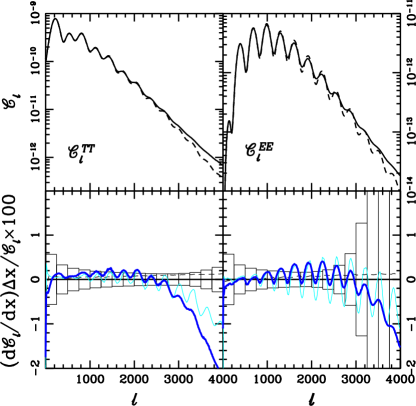
Figure 1: Top panels: angular power spectra ${\cal C}_{l}^{TT}$ (left) and ${\cal C}_{l}^{EE}$ (right) for the fiducial model ($m_{\nu}=0$) with no lensing (dashed) and with lensing (solid). Bottom panels: $100\times d{\cal C}_{l}^{TT}/dm_{\nu}\times(\Delta m_{\nu}/{\cal C}_{l}^{TT})$ (dark) and $100\times d{\cal C}_{l}^{TT}/dw_{X}\times(\Delta w_{X}/{\cal C}_{l}^{TT})$ (light) for $\Delta m_{\nu}=0.1$ eV and $\Delta w_{X}=0.2$. Same for ${\cal C}_{l}^{EE}$.

Lensing introduces calculable non-gaussianities into the CMB temperature maps bernardeau97 ; zaldarriaga00a ; okamoto02 ; cooray03 . Lets denote the fourier transform on the sky of measured CMB maps by $a^{X}(\vec{l})$, $X=\{T,E,B\}$, the corresponding unlensed (unobserved) maps by $\tilde{a}^{X}(\vec{l})$, and their two point functions by ${\cal C}_{l}^{XX^{\prime}}\equiv\langle a^{X}(\vec{l})a^{X^{\prime}}(\vec{l})\rangle l(l+1)/2\pi$ and $\tilde{\cal C}_{l}^{XX^{\prime}}\equiv\langle\tilde{a}^{X}(\vec{l})\tilde{a}^{X^{\prime}}(\vec{l})\rangle l(l+1)/2\pi$. In real space lensing simply shifts a photon from one part of the sky to another by a small angle (typically $\sim$ arcminutes). In fourier transform space that implies $\langle a^{X}(\vec{l})a^{X^{\prime}}(\vec{l}^{\prime})\rangle=f_{XX^{\prime}}(\vec{l},\vec{l}^{\prime})d(\vec{l}+\vec{l}^{\prime})$ which can be used to estimate the deflection angle $d(\vec{L})$ hu02b given an estimate of the unlensed two-point functions. The power spectrum of the deflection angle is plotted in the top panel of Fig. 2 along with the power spectrum of the scalar B-mode polarization (created by lensing).

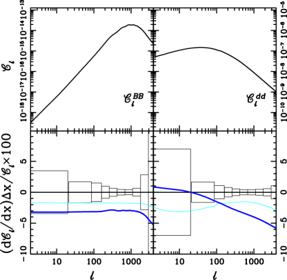
Figure 2: Top panels: angular power spectra ${\cal C}_{l}^{BB}$ with no tensor contribution (left) and ${\cal C}_{l}^{dd}$ (right) for the fiducial model ($m_{\nu}=0$). Bottom panels: same as for Fig. 1 but for $C_{l}^{BB}$ and ${\cal C}_{l}^{dd}$.

Lensing and Absolute Neutrino Masses. Without the effect of lensing, Eisenstein et al. eisenstein99 found that the Planck satellite can measure neutrino mass with an error of 0.26 eV. This sensitivity limit is related to the temperature of the recombination surface $T_{\rm rec}\simeq 0.3$ eV. Neutrinos with $m_{\nu}\mathrel{\mathchoice{\lower 3.6pt\vbox{\halign{$\mathsurround=0pt\displaystyle\hfil#\hfil$\cr<\crcr\sim\crcr}}}{\lower 3.6pt\vbox{\halign{$\mathsurround=0pt\textstyle\hfil#\hfil$\cr<\crcr\sim\crcr}}}{\lower 3.6pt\vbox{\halign{$\mathsurround=0pt\scriptstyle\hfil#\hfil$\cr<\crcr\sim\crcr}}}{\lower 3.6pt\vbox{\halign{$\mathsurround=0pt\scriptscriptstyle\hfil#\hfil$\cr<\crcr\sim\crcr}}}}T_{\rm dec}$ do not leave imprints on the recombination surface that would distinguish them from $m_{\nu}=0$.

Neutrinos with mass $m_{\nu}\mathrel{\mathchoice{\lower 3.6pt\vbox{\halign{$\mathsurround=0pt\displaystyle\hfil#\hfil$\cr<\crcr\sim\crcr}}}{\lower 3.6pt\vbox{\halign{$\mathsurround=0pt\textstyle\hfil#\hfil$\cr<\crcr\sim\crcr}}}{\lower 3.6pt\vbox{\halign{$\mathsurround=0pt\scriptstyle\hfil#\hfil$\cr<\crcr\sim\crcr}}}{\lower 3.6pt\vbox{\halign{$\mathsurround=0pt\scriptscriptstyle\hfil#\hfil$\cr<\crcr\sim\crcr}}}}T_{\rm rec}$ would, however, affect the evolution of the inhomogeneities. To understand the effects we need to study the comoving Jeans length for the neutrinos $\lambda_{J}(a)$. This length scale is set by the competition between the pressure due to the velocity dispersion of neutrinos and gravity. For non-relativistic neutrinos in a matter dominated universe $\lambda_{J}(a)\propto m_{\nu}^{-1}a^{-1/2}$ bond83 ; ma96 ; hu98 . Note that the comoving Jeans length was much larger in the past. For $k\mathrel{\mathchoice{\lower 3.6pt\vbox{\halign{$\mathsurround=0pt\displaystyle\hfil#\hfil$\cr<\crcr\sim\crcr}}}{\lower 3.6pt\vbox{\halign{$\mathsurround=0pt\textstyle\hfil#\hfil$\cr<\crcr\sim\crcr}}}{\lower 3.6pt\vbox{\halign{$\mathsurround=0pt\scriptstyle\hfil#\hfil$\cr<\crcr\sim\crcr}}}{\lower 3.6pt\vbox{\halign{$\mathsurround=0pt\scriptscriptstyle\hfil#\hfil$\cr<\crcr\sim\crcr}}}}k_{J}(a)\equiv 1/\lambda_{J}(a)$, neutrinos can cluster like dark matter. On smaller scales, neutrinos do not fall into dark matter potential wells.

The above discussion helps us understand the changes to the dark matter perturbation evolution seen in Fig. 3. On the smallest scales in Fig. 3, there is a uniform suppression because neutrinos never cluster hu98 . On scales larger than the Jeans length today, ${\cal O}({\rm Mpc})$ for $m_{\nu}={\cal O}({\rm eV})$, neutrinos do cluster once $k\mathrel{\mathchoice{\lower 3.6pt\vbox{\halign{$\mathsurround=0pt\displaystyle\hfil#\hfil$\cr<\crcr\sim\crcr}}}{\lower 3.6pt\vbox{\halign{$\mathsurround=0pt\textstyle\hfil#\hfil$\cr<\crcr\sim\crcr}}}{\lower 3.6pt\vbox{\halign{$\mathsurround=0pt\scriptstyle\hfil#\hfil$\cr<\crcr\sim\crcr}}}{\lower 3.6pt\vbox{\halign{$\mathsurround=0pt\scriptscriptstyle\hfil#\hfil$\cr<\crcr\sim\crcr}}}}k_{J}(a)$. This accounts for the increase in $\delta_{m}$ from about 10 Mpc to about 100 Mpc. For scales much larger than the Jeans length at matter-radiation equality, which is ${\cal O}(100{\rm Mpc})$ for $m_{\nu}={\cal O}({\rm eV})$, the neutrinos can always cluster after horizon crossing. In this regime the suppression of the dark matter perturbation comes from the change in the overall growth factor because the addition of a massive neutrino speeds up the expansion rate of the universe.

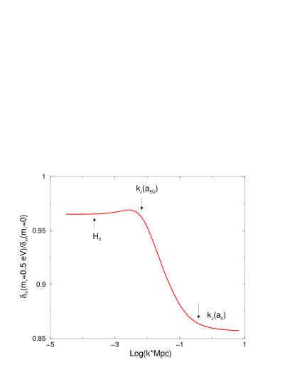
Figure 3: Effect of a massive neutrino on dark matter perturbation. The fiducial model has three massless neutrinos, one of which is given a mass of 0.5 eV. Scales corresponding to the Jeans length at equality ($a=a_{\rm EQ}$) and today ($a=a_{0}$), as well as the Hubble horizon today are labeled.

The amplitude of dark matter perturbations determines the fluctuations in the metric $\Phi$ which in turn feeds into the lensing deflection angle as $d(\vec{L})=\sqrt{L(L+1)}\phi(\vec{L})$. $\phi(\vec{L})$ is the fourier transform on the sky of $\phi(\vec{\theta})=2\int d\chi\Phi(\vec{\theta}\chi,\chi)(\chi_{\rm rec}-\chi)/(\chi\chi_{\rm rec})$ where the integration is along the unperturbed geodesic of the photon. We will denote the three dimensional power spectrum of the metric perturbation $\Phi$ by $P_{\Phi}(k)$.

The lower panels in Figs. 1 and 2 show the differences in the power spectra when one of the three neutrinos is given a mass of 0.1 eV. The error boxes are those for CMBpol (described below; see Table I). Note that the signature of a 0.1 eV neutrino in the angular power spectra, in the absence of lensing, is at the 0.1% level as shown in Fig. 1.

Limits on Neutrino Mass. Presently, the most stringent laboratory upper bound on neutrino mass comes from tritium beta decay end-point experiments tritium which limit the electron neutrino mass to $\mathrel{\mathchoice{\lower 3.6pt\vbox{\halign{$\mathsurround=0pt\displaystyle\hfil#\hfil$\cr<\crcr\sim\crcr}}}{\lower 3.6pt\vbox{\halign{$\mathsurround=0pt\textstyle\hfil#\hfil$\cr<\crcr\sim\crcr}}}{\lower 3.6pt\vbox{\halign{$\mathsurround=0pt\scriptstyle\hfil#\hfil$\cr<\crcr\sim\crcr}}}{\lower 3.6pt\vbox{\halign{$\mathsurround=0pt\scriptscriptstyle\hfil#\hfil$\cr<\crcr\sim\crcr}}}}2$ eV. Several proposed experiments plan to reduce this limit by one to two orders of magnitude by searching for neutrino-less double beta decay ($\beta\beta 0\nu$) zdesenko03 . A Dirac mass would elude this search, but theoretical prejudice favors (and the see-saw mechanism requires) Majorana masses. The theoretical uncertainties associated with $\beta\beta 0\nu$ experiments are large vergados02 but this is the only way to ascertain if the neutrino is a Majorana particle. Like the CMB and galaxy shear observations, these future $\beta\beta 0\nu$ experiments will be extremely challenging. We note that galaxy shear observations have the potential to be competitive with the CMB and $\beta\beta 0\nu$ experiments in putting limits on the neutrino mass hu99 ; abazajian02b .

Lensing and Dark Energy. Dark energy affects lensing in two distinct ways. First, the presence of dark energy implies faster expansion and hence a decrease in the overall growth rate. Second, dark energy can cluster appreciably on scales $k\mathrel{\mathchoice{\lower 3.6pt\vbox{\halign{$\mathsurround=0pt\displaystyle\hfil#\hfil$\cr>\crcr\sim\crcr}}}{\lower 3.6pt\vbox{\halign{$\mathsurround=0pt\textstyle\hfil#\hfil$\cr>\crcr\sim\crcr}}}{\lower 3.6pt\vbox{\halign{$\mathsurround=0pt\scriptstyle\hfil#\hfil$\cr>\crcr\sim\crcr}}}{\lower 3.6pt\vbox{\halign{$\mathsurround=0pt\scriptscriptstyle\hfil#\hfil$\cr>\crcr\sim\crcr}}}}k_{Q}\equiv 2V_{,QQ}^{-1/2}$ ma99 where we have modeled dark energy as a scalar field $Q$ with effective mass $V_{,QQ}^{1/2}$ which is ${\cal O}(H_{0})$. The clustering of dark energy boosts the metric perturbations and hence lensing. However, if the dark energy equation of state $w_{X}$ ($p_{X}=w_{X}\rho_{X}$ with $X$ denoting the dark energy component) is close to -1, then the perturbations in the dark energy density are not important. The effect of a change in $w_{X}$ is shown in Fig. 4.

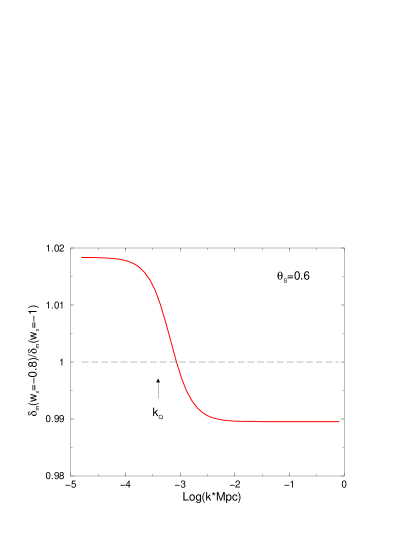
Figure 4: Effect on the dark matter perturbation of a change in the dark energy equation of state from $w_{X}=-1$ to $w_{X}=-0.8$.

The $l$-dependence of $\partial\ln{\cal C}_{l}^{dd}/\partial w_{X}$ is different from that of $\partial\ln{\cal C}_{l}^{dd}/\partial m_{\nu}$ (see Fig. 2). As mentioned, the primary effect is due to a suppression of the overall growth factor and hence the effect of $w_{X}$ on ${\cal C}_{l}^{dd}$ is not strongly $l$-dependent. Note that the effect of $w_{X}$ will be more pronounced for larger values of $w_{X}$ due to two reasons. One, dark energy starts to dominate earlier (which implies larger uniform suppression) and two, perturbations in dark energy on large scales are enhanced for large $w_{X}$.

The CMB lensing window function is fairly broad in redshift–space. A downside of this is the fact that CMB lensing will never be competitive with SNIa observations (and possibly cosmic shear) as far as measuring $w_{X}$ is concerned. However, the virtue of CMB lensing is that it would be a robust alternative probe of the acceleration of the universe and that the physics is different from that of SNIa since lensing is sensitive to both the growth of perturbations and distances. The sensitivity to a broad range of redshifts also implies that CMB lensing is a unique probe of dark energy (more generally clustering) at $z\mathrel{\mathchoice{\lower 3.6pt\vbox{\halign{$\mathsurround=0pt\displaystyle\hfil#\hfil$\cr>\crcr\sim\crcr}}}{\lower 3.6pt\vbox{\halign{$\mathsurround=0pt\textstyle\hfil#\hfil$\cr>\crcr\sim\crcr}}}{\lower 3.6pt\vbox{\halign{$\mathsurround=0pt\scriptstyle\hfil#\hfil$\cr>\crcr\sim\crcr}}}{\lower 3.6pt\vbox{\halign{$\mathsurround=0pt\scriptscriptstyle\hfil#\hfil$\cr>\crcr\sim\crcr}}}}2$. We also note that if $w_{X}$ is demonstrably different from -1, then dark energy must cluster on 1000 Mpc scales. The clustering properties of dark energy, say parameterized in terms of it sound speed, might then be measurable.

Reionization, Optical Depth and Primordial Power Spectrum. Reionization of the universe happened sometime between the redshifts of 30 and 6.3. The lower bound comes from the observation of the Gunn-Peterson trough in a $z=6.3$ quasar becker01 . The upper bound comes from the upper limit to the value of the optical depth to Thomson scattering, denoted by $\tau$, for photons from WMAP TE two-point function measurements kogut03 .

The CMB photons scatter off of the energetic free electrons produced during reionization of the universe and this leaves an imprint on their anisotropy which allows us to study the end of dark ages (the era before the first stars turned on). A measurement of the optical depth also allows us to determine the amplitude of the primordial power spectrum $P_{\Phi}^{i}$ better. The overall power of the primary CMB anisotropy on scales $l\mathrel{\mathchoice{\lower 3.6pt\vbox{\halign{$\mathsurround=0pt\displaystyle\hfil#\hfil$\cr>\crcr\sim\crcr}}}{\lower 3.6pt\vbox{\halign{$\mathsurround=0pt\textstyle\hfil#\hfil$\cr>\crcr\sim\crcr}}}{\lower 3.6pt\vbox{\halign{$\mathsurround=0pt\scriptstyle\hfil#\hfil$\cr>\crcr\sim\crcr}}}{\lower 3.6pt\vbox{\halign{$\mathsurround=0pt\scriptscriptstyle\hfil#\hfil$\cr>\crcr\sim\crcr}}}}100$ is set by the combination $P_{\Phi}^{i}\exp(-\tau)$. It is this combination that present CMB observations constrain well. Any information about $\tau$ therefore breaks this $\tau$–$P_{\Phi}^{i}$ degeneracy and allows for a determination of the primordial power spectrum amplitude.

The scattering of CMB photons after reionization changes the primary anisotropy at large angles or low $\ell$ corresponding to the horizon during reionization zaldarriaga97b . This change is not evident in the TT power spectrum because of the dominant Sachs-Wolfe effect at low $\ell$. However, there is no analog of the Sachs-Wolfe effect for polarization and hence any new anisotropy produced at the “reionization surface” should be measurable through the TE and EE power spectrum at low $\ell$. This bump in the power at low $\ell$ has been recently measured by the WMAP team kogut03 which allowed them to ascertain that the universe was first reionized at $z\sim 20$.

Planck should measure this low $\ell$ signal much better. A theoretical limiting factor to how well $\tau$ can be measured is our ignorance about the reionization history kaplinghat02a ; hu03 (i.e., evolution of the ionized hydrogen fraction between redshifts of 6 and 30). It was recently shown holder03 that including this ignorance implies that the 1-$\sigma$ error on $\tau$ from Planck should be about 0.005 which implies that the amplitude of the primordial power spectrum will be measured to about 1%.

Lensing and Primordial Power Spectrum. Another way to break the $\tau$-$P_{\Phi}^{i}$ degeneracy is through the small scale lensing signal hu02a . Note that due to lensing the power spectra do not scale as $P_{\Phi}^{i}$ on small scales. If lensing were the dominant contribution to the two point functions, then measured two point functions would scale as $(P_{\Phi}^{i})^{2}$. In addition, on small scales, one has to include the effect of non-linear evolution of the density perturbations which have more complicated dependence on $P_{\Phi}^{i}$. Thus precision measurements of the small scale CMB power can in fact measure $P_{\Phi}^{i}$ and thus provide an indirect measurement of the optical depth. This effect would be important if, for example, the low $\ell$ reionization bump cannot be measured well.

Measuring the lensing signal requires high angular resolution. Along with the lensing signal we can also estimate the primary CMB signal out to small scales. This is very useful for measuring the scale-dependence of the primordial power spectrum. In particular if we take the primordial power spectrum to be $k^{3}P_{\Phi}^{i}(k)=k_{f}^{3}P_{\Phi}^{i}(k_{f})(k/k_{f})^{n_{S}-1+n_{S}^{\prime}\ln(k/k_{f})}$ with $k_{f}=0.05/{\rm Mpc}$, then future CMB experiments can provide a precision measurement of $n_{S}$ and $n_{S}^{\prime}$ (derivative of $n_{S}$ with respect to $\ln(k)$). In the context of inflationary models we expect $n_{S}^{\prime}\sim(n_{S}-1)^{2}$. An experiment like CMBpol will be able to test this relation if $|n_{S}-1|\mathrel{\mathchoice{\lower 3.6pt\vbox{\halign{$\mathsurround=0pt\displaystyle\hfil#\hfil$\cr>\crcr\sim\crcr}}}{\lower 3.6pt\vbox{\halign{$\mathsurround=0pt\textstyle\hfil#\hfil$\cr>\crcr\sim\crcr}}}{\lower 3.6pt\vbox{\halign{$\mathsurround=0pt\scriptstyle\hfil#\hfil$\cr>\crcr\sim\crcr}}}{\lower 3.6pt\vbox{\halign{$\mathsurround=0pt\scriptscriptstyle\hfil#\hfil$\cr>\crcr\sim\crcr}}}}5\%$.

Lensing, Reionization and Gravity Waves from Inflation. The primary motivation for a full-sky mission after Planck, see CMBpol in Table I, is the detection of the B mode due to gravity waves produced in inflation. The amplitude of this signal would directly give us the energy density during inflation. At small scales this primordial (tensor) B mode signal will be overwhelmed by the scalar B mode signal unless the ratio of the primordial tensor to scalar power spectrum amplitudes is larger than about 1%. The scalar B mode signal arises because (as we discussed before) lensing converts some E mode polarization to B modes. Following the calculation in knox02 (see also kesden02 ) we find a $3\sigma$ detection is possible for CMBpol if the fourth root of the energy density during inflation is greater than $E_{\rm min}=2\times 10^{15}$ GeV which is an order of magnitude smaller than the GUT scale. We note that $E_{\rm min}^{4}\propto 1/\tau$, approximately, for $0.05<\tau<0.2$ and we have assumed $\tau=0.1$. This scaling with $\tau$ suggests that the largest angular scales, where the reionization feature in the B mode appears, are important and therefore a full-sky experiment is necessary to achieve this sensitivity level.

Recombination, Helium Mass Fraction and BBN. The free electron fraction during recombination depends on the helium mass fraction $Y_{P}$. Thus a change in the helium mass fraction changes the visibility function at the recombination surface and hence the primary CMB power spectra. This implies that by measuring the acoustic peaks out to $\ell\sim 1000$ well, one can determine the helium mass fraction. In order to reach that conclusion, we have to assume that the standard recombination physics is correct which would not be the case, for example, if the fine structure constant was different at the recombination surface kaplinghat99 .

Thus, along with the baryon density, future CMB experiments will be able to determine $Y_{P}$ to high precision. This will facilitate precision consistency tests with Big Bang Nucleosynthesis (BBN) predictions. It will also be useful in constraining non-standard BBN. For example, determining baryon density and helium mass fraction to high precision allows strong constraints to be put on the number of relativistic species N (or equivalently the expansion rate) during BBN. If $\sigma(Y_{P})$ is small, then $\sigma(N)=\sigma(Y_{P})/0.013$, which for CMBpol works out to $\sigma(N)=0.2$. Constraints on $N$ have important repercussions for neutrino mixing in the early universe, and hence on neutrino mass models abazajian02 .

Experiment	$l_{\rm max}^{\rm UL}$	$l_{\rm max}^{\rm T}$	$l_{\rm max}^{\rm E,B}$	$\nu$ (GHz)	$\theta_{b}$	$\Delta_{T}$	$\Delta_{P}$
Planck	2000	2000	2500	100	9.2’	5.5	$\infty$
				143	7.1’	6	11
				217	5.0’	13	27
SPTpol ($f_{\rm sky}=0.1$)	2000	2000	2500	217	0.9’	12	17
CMBpol	2000	2000	2500	217	3.0’	1	1.4

Table 1: Experimental specifications. Unlensed spectra (${\tilde{\cal C}}_{l}^{TT}$, ${\tilde{\cal C}}_{l}^{TE}$, ${\tilde{\cal C}}_{l}^{EE}$) limited to $l<l_{\rm max}^{\rm UL}$. $\phi$ reconstruction using only $l<l_{\rm max}^{T,E,B}$ lensed spectra.

Table 2:

Error Forecasts
Experiment $m_{\nu}$ (eV) $w_{x}$ $\ln P_{\Phi}^{i}$ $n_{S}$ $n_{S}^{\prime}$ $\theta_{s}$ (deg) $\tau$ $\ln\omega_{m}$ $\ln\omega_{b}$ $Y_{P}$ Planck 0.15 0.31 0.017 0.0071 0.0032 0.002 0.0088 0.0066 0.0075 0.012 SPTpol 0.18 0.49 0.018 0.01 0.006 0.0026 0.0088 0.0087 0.01 0.017 CMBpol 0.044 0.18 0.017 0.0029 0.0017 0.00064 0.0085 0.0022 0.0028 0.0048
Notes.—Standard deviations expected from Planck, SPTpol and CMBpol.

Error Forecasting. The experiments we consider are Planck planck , a mission concept for a future full-sky mission called CMBpol , and a polarized bolometer array on the South Pole Telescope we will call SPTpol. Their specifications are given in Table I. We assume that other frequency channels of Planck and CMBpol (not shown in Table I) will clean out non-CMB sources of radiation perfectly. Detailed studies have shown foreground degradation of the results expected from Planck to be mild knox99 ; tegmark00b ; bouchet99 . We have restricted the range of the power spectra keeping in mind that at small scales foregrounds are likely to be an issue. Certainly at $l\mathrel{\mathchoice{\lower 3.6pt\vbox{\halign{$\mathsurround=0pt\displaystyle\hfil#\hfil$\cr>\crcr\sim\crcr}}}{\lower 3.6pt\vbox{\halign{$\mathsurround=0pt\textstyle\hfil#\hfil$\cr>\crcr\sim\crcr}}}{\lower 3.6pt\vbox{\halign{$\mathsurround=0pt\scriptstyle\hfil#\hfil$\cr>\crcr\sim\crcr}}}{\lower 3.6pt\vbox{\halign{$\mathsurround=0pt\scriptscriptstyle\hfil#\hfil$\cr>\crcr\sim\crcr}}}}3000$ once can expect emission from dusty galaxies to be a significant contaminant. Other foregrounds like those due to kinetic SZ effect from patchy reionization will also be severe at $l\mathrel{\mathchoice{\lower 3.6pt\vbox{\halign{$\mathsurround=0pt\displaystyle\hfil#\hfil$\cr>\crcr\sim\crcr}}}{\lower 3.6pt\vbox{\halign{$\mathsurround=0pt\textstyle\hfil#\hfil$\cr>\crcr\sim\crcr}}}{\lower 3.6pt\vbox{\halign{$\mathsurround=0pt\scriptstyle\hfil#\hfil$\cr>\crcr\sim\crcr}}}{\lower 3.6pt\vbox{\halign{$\mathsurround=0pt\scriptscriptstyle\hfil#\hfil$\cr>\crcr\sim\crcr}}}}3000$, and may even dominate the lensing signal knox98 ; santos03 . However, these effects are less severe in polarization. We note that the results for CMBpol are not significantly affected if we restrict temperature data to $l<1000$.

The power spectra we include in our analysis are ${\tilde{\cal C}}_{l}^{TT}$, ${\tilde{\cal C}}_{l}^{TE}$, ${\tilde{\cal C}}_{l}^{EE}$ (unlensed), and ${\cal C}_{l}^{dd}$. We do not use the lensed power spectra to avoid the complication of the correlation in their errors between different $\ell$ values and with the error in ${\cal C}_{l}^{dd}$. Using the lensed spectra and neglecting these correlations can lead to overly optimistic forecasts hu02a .

The error forecasting method jungman96 ; bond97 is based on the fisher matrix formalism. Care must be exercised in calculating the derivatives with respect to parameters like $w_{X}$ and $m_{\nu}$ since their effects are small, and predominantly through lensing, once their effect on the angular diameter distance is taken out. In particular, the angle subtended by the sound horizon at the recombination surface, $\theta_{s}$, must be included as one of the parameters since it will be measured with exquisite precision. We take our parameter set to be ${\cal P}=\{\omega_{m},\omega_{b},\omega_{\nu},\theta_{s},w_{X},z_{\rm ri},k^{3}P_{\Phi}^{i}(k_{f}),n_{s},n_{s}^{\prime},Y_{P}\}$. The first three of these are the densities today (in units of $1.88\times 10^{-29}{\rm g}/{\rm cm}^{3}$) of cold dark matter plus baryons, baryons and massive neutrinos. Note that for one massive neutrino, $\omega_{\nu}=m_{\nu}/94.2{\rm eV}$. The Thompson scattering optical depth for CMB photons, $\tau$, is parameterized by the redshift of reionization $z_{\rm ri}$. We Taylor expand about ${\cal P}=\{0.146,0.021,0,0.6,-1,6.3,6.4\times 10^{-11},1,0,0.24\}$. See kaplinghat03c for more details on the error forecasting method.

Results. The results are summarized in Table II and we list the salient features here. Planck has the potential to measure the amplitude of the scalar primordial power spectrum to about 1% and inform us about the end of dark ages by using the boost in power at low multipoles in the CMB polarization due to reionization. For all entries in Table II we have assumed this as prior knowledge and not included the low multipoles in the analysis.

Gravitational lensing of the CMB is clearly a promising probe of the growth of structure and the fundamental physics that affects it. CMBpol can provide evidence for the acceleration of the universe, independent of SNIa observations. It can throw light on inflationary dynamics by testing for consistency with the relation $n_{S}^{\prime}\sim(n_{S}-1)^{2}$. The most striking result in Table II is the promise that cosmology can provide us with an absolute determination of neutrino mass to about 0.04 eV. We can be optimistic that a future all-sky polarized CMB mission aimed at detecting gravitational waves is likely to succeed in determining neutrino mass as well.

Acknowledgments. This article is based on work done in collaboration with Lloyd Knox and Yong-Seon Song, and I would like to thank both my collaborators. I would also like to thank Wayne Hu for helpful discussions.

References

- (1) C. L. Bennett et al., (2003), astro-ph/0302207.
- (2) M. Kaplinghat, L. Knox, and Y.-S. Song, (2003), astro-ph/0303344.
- (3) M. Zaldarriaga and U. . Seljak, Phys. Rev. D58, 023003 (1998).
- (4) F. Bernardeau, Astron. & Astrophys.324, 15 (1997).
- (5) M. Zaldarriaga, Phys. Rev. D62, 63510 (2000).
- (6) T. Okamoto and W. Hu, Phys. Rev. D66, 63008 (2002).
- (7) A. Cooray and M. Kesden, New Astronomy 8, 231 (2003).
- (8) W. Hu and T. Okamoto, Astrophys. J. 574, 566 (2002).
- (9) D. J. Eisenstein, W. Hu, and M. Tegmark, Astrophys. J. 518, 2 (1999).
- (10) J. R. Bond and A. S. Szalay, Astrophys. J. 274, 443 (1983).
- (11) C. Ma, Astrophys. J. 471, 13 (1996).
- (12) W. Hu and D. J. Eisenstein, Astrophys. J. 498, 497 (1998).
- (13) J. Bonn et al., Nucl. Phys. Proc. Suppl. 110, 395 (2002).
- (14) Y. Zdesenko, Rev. Mod. Phys. 74, 663 (2003).
- (15) J. D. Vergados, Phys. Rept. 361, 1 (2002).
- (16) W. Hu, Astrophys. J. Lett.522, L21 (1999).
- (17) K. N. Abazajian and S. Dodelson, (2002), astro-ph/0212216.
- (18) C. Ma, R. R. Caldwell, P. Bode, and L. Wang, Astrophys. J. Lett.521, L1 (1999).
- (19) R. H. Becker et al., Astron. J.122, 2850 (2001).
- (20) A. Kogut et al., (2003), astro-ph/0302213.
- (21) M. Zaldarriaga, Phys. Rev. D55, 1822 (1997).
- (22) M. Kaplinghat et al., Astrophys. J. 583, 24 (2003).
- (23) W. Hu and G. P. Holder, Phys. Rev. D. 68, 023001 (2003).
- (24) G. Holder, Z. Haiman, M. Kaplinghat, and L. Knox, (2003), astro-ph/0302404.
- (25) W. Hu, Phys. Rev. D65, 23003 (2002).
- (26) L. Knox and Y.-S. Song, Phys. Rev. Lett. 89, 011303 (2002).
- (27) M. Kesden, A. Cooray, and M. Kamionkowski, Phys. Rev. Lett. 89, 11304 (2002).
- (28) M. Kaplinghat, R. J. Scherrer, and M. S. Turner, Phys. Rev. D60, 023516 (1999).
- (29) K. N. Abazajian, (2002), astro-ph/0205238.
- (30) J. A. Tauber, in IAU Symposium (PUBLISHER, ADDRESS, 2001), pp. 493–+.
- (31) L. Knox, Mon.Not.Roy.As.Soc.307, 977 (1999).
- (32) M. Tegmark, D. J. Eisenstein, W. Hu, and A. de Oliveira-Costa, Astrophys. J. 530, 133 (2000).
- (33) F. R. Bouchet and R. Gispert, New Astronomy 4, 443 (1999).
- (34) L. Knox, R. . Scoccimarro, and S. Dodelson, Phys. Rev. Lett. 81, 2004 (1998).
- (35) M. G. Santos et al., (2003), astro-ph/0305471.
- (36) G. Jungman, M. Kamionkowski, A. Kosowsky, and D. N. Spergel, Phys. Rev. D54, 1332 (1996).
- (37) J. R. Bond, G. Efstathiou, and M. Tegmark, Mon. Not. Roy. Astron. Soc. 291, L33 (1997).