Homogeneity of early–type galaxies across clusters

We studied the homogeneity, across clusters, of the color of the red sequence (the intercept of the color–magnitude relation) of 158 clusters and groups detected in the Early Data Release of the Sloan Digital Sky Survey (EDR–SDSS) in the redshift range $0.06<z<0.34$. We found a high degree of homogeneity: the color of the red sequence shows an intrinsic scatter of 0.02 mag across clusters, suggesting that either galaxies on the red sequence formed a long time ago ($z>2$) or else their star formation is universally delayed with preservation of a small spread in age formation. The latter possibility is ruled out by the mere existence of galaxies at high redshift. While the old age of ellipticals was already been claimed for a small heterogeneous collection of clusters, most of which are rich ones, we found that it holds for ten to one hundred large sample, representative of all clusters and groups detected on the EDR–SDSS. Hence we suggest the possible universality of the color of the galaxies on the red sequence. Furthermore, the sample includes a large number of very poor clusters (also called groups), not studied in previous works, for which the hierarchical and monolithic scenarios of elliptical formation predict different colors for the brightest ellipticals. The observed red sequence color does not depend on cluster/group richness at a level of 0.02 mag, while a $\sim 0.23$ mag effect is expected according to the hierarchical prediction. Therefore, the stellar population of red sequence galaxies is similar in clusters and groups, in spite of different halo histories. Finally, since the observed rest–frame color of the red sequence does not depend on environment and redshift, it can be used as a distance indicator, with an error $\sigma_{z}=0.018$, a few time better than the precision achieved by other photometric redshift estimates and twice better than the precision of the Fundamental Plane for a single galaxy at the median redshift of the EDR–SDSS.

1 Introduction

The existence of a relation between color and magnitude for early type galaxies is known since a long time (e.g. Sandage & Visvanathan 1978). This relation, known as color–magnitude relation, implies a link between the mass of the stellar population and its age or metallicity, with the latter being the presently favored explication, because high redshift clusters have bluer (rest–frame) color–magnitude relations with a small scatter (Ellis et al. 1997, Kodama & Arimoto 1997, Stanford, Eisenhardt & Dickinson 1998; Kodama 1998). The color–magnitude relation, often called red sequence, of different clusters shows an homogeneity across clusters, in the sense that the (rest–frame) color of the red sequence is similar for the presently studied clusters (e.g. Garilli et al. 1996), although the sample studied thus far presents several limitations described in the next paragraph. A color uniformity, inside each cluster or across different clusters, implies that stellar populations are similar, or old enough that differences induced by a spread in formation ages are dumped out.

At first sight, the early formation of the bulk of stars in cluster galaxies seems a problem for hierarchical scenarios of galaxy formation. However, while star formation occurs late in such a models, it is pushed back to early times in clusters (Kauffmann 1996). Hence the conclusion that in clusters the bulk of stars in galaxies is homogeneous and red is not in contradiction with the hierarchical scenario. A natural consequence of hierarchical models would be that the evolution of early–type galaxies should depend on their environment: merging history are likely to have varied from cluster to groups, and also across groups because they are formed by the coalescence of a tiny number of halos.

From the observational side, Bower, Lucey & Ellis (1992), Aragon-Salamanca et al. (1993), Ellis et al. (1997), Stanford, Eisenhardt & Dickinson (1998), Kodama et al. (1998), all studied the homogeneity of the color of the red sequence in 2, 10, 3, 19, 17 clusters, respectively, with the latter paper drawing data from previous papers and performing a comprehensive analysis of the same observational data. All but two studied clusters are rich or very rich. Rich clusters are the ones for which a hierarchical scenario and the usual monolithic scenario for elliptical formation (Eggen, Lynden-Bell & Sandage 1962) give the same prediction about early–type color and dispersion around the color–magnitude relation (Kauffmann & Charlot 1998) and hence rich clusters cannot be used to discriminate between the two scenario. Finally, the clusters studied thus far are mostly at intermediate redshift ($z>0.3$), and therefore our local universe is mostly unexplored in this sense.

To summarize, the sample studied thus far is an heterogeneous collection of clusters, and not a representative sample of clusters in the Universe. Hence, what we know on the homogeneity of ellipticals is mainly based on a restricted number of rich clusters, mostly at high redshift, selected in an uncontrolled way.

In this paper we present mainly an observational effort to study a sample:

-that is larger (by a factor 10 to 100) than previous works;

-that is a representative sample of local clusters and groups detected in the Sloan Digital Sky Survey;

-that spans a broad range in richness, including groups, hence allowing us to discriminate between monolithic and hierarchical scenarios of elliptical formation.

Section 2 presents the cluster sample and the data used. Observational results are presented in section 3 and are summarized and discussed in section 4. In section 5 we model the star formation history of the clusters and compare it with the observations. Finally, section 6 summarizes the conclusions.

All along the paper we use robust statistics, even if we refrain ourselves to remind it. In place of the mean we use the median, and in place of the dispersion we use 1.47 times the interquartile range (the coefficient is appropriate for a Gaussian distribution), but we still call them “mean” and “dispersion”, respectively.

No cosmological model is needed in the analysis of Section 2 and 3, while a “concordance” model ($H_{0}=70$ km s^-1 Mpc^-1, $\Omega_{m}=0.3$ and $\Omega_{\Lambda}=0.7$) is used for conversion from times to redshift in Section 5. In the course of the Section 4 absolute quantities (such as absolute magnitudes or metric radii) are mentioned using $H_{0}=50$ km s^-1 Mpc^-1 for allowing an immediate comparison with published results derived in the “standard” model, but the important quantities are the apparent ones, that are independent on the cosmological parameters.

2 Data & Method

The aim of this section is to measure the color of the red sequence in a large sample of groups and clusters. To this aim, we present the galaxy catalog, the detection algorithm used to detect clusters and groups, the way we measure redshifts of our clusters and groups, and the biases induced by the detection algorithm and by the redshift determination, with particular emphasis on those potentially discarding clusters having a red sequence with color different from the average.

2.1 The galaxy catalog & the cluster detection algorithm

We used the Early Data Release of the Sloan Digital Sky Survey (EDR–SDSS) catalog (Stoughton et al. 2002), of which we considered a sub–area of 294.6 deg² having a rectangular shape. The galaxy catalog have been filtered out by residual stellar contamination and by saturated objects, as described in Andreon (2003). $g^{\prime}-r^{\prime}$ color has been computed using fiber (3 arcsec aperture) magnitudes. All magnitudes and colors have been corrected for Galactic absorption, using the extinction values listed in the EDR–SDSS database. Only galaxies brighter than $r_{Petro}=21.5$ mag are considered ($M^{*}+2$ at $z=0.3$ for unevolving early–type galaxies, assuming the $M^{*}$ value quoted in Blanton et al. 2001).

Clusters of galaxies have been detected by a method inspired to, but fundamentally different from, Gladders & Yee (2000) and fully described in Andreon (2003). Shortly, the method takes advantage from the observed fact that most of galaxies in clusters shares similar colors, while background galaxies have a variety of colors, both because they are spread over a larger redshift range and because the field population is more variegated in color than the cluster one, even at a fixed redshift. In practice, the method looks at spatially localized galaxy overdensities of similar color. It works because the filtering in color reduces the background galaxies (which have a variety of colors) without completing discarding the cluster contribution. Being the cluster search almost in three dimensions (color plus two spatial directions), projection effects that plagued previous two dimensional searches are strongly reduced.

For each color slice, whose central color is made to vary in order to detect galaxy overdensities at different colors, a multiscale detection algorithm is applied to the map of the numerical density of galaxies. By a friend–of–friend algorithm, detections at different scales and colors are then grouped together when they overlap in sky and in color. The “winner” detection is the one that maximizes the numerical density of galaxies.

We applied the cluster detection algorithm, using a 0.1 mag wide strip in color, stepped by half its width, and 2.5, 5 and 10 arcmin boxes, stepped by half their width. The catalog used in this paper is drawn from the one formed by the 643 statistically most significant detections, defined here as those having a probability smaller than $10^{-6}$ to be statistical fluctuations. The size of the “winner” detection has the mode at $\sim 500$ kpc, the minimum at $\sim 200$ kpc and a tail up to 4 Mpc.

Our detection algorithm does not bias the catalog against clusters having galaxies with abnormal color (e.g. with a color–magnitude relation having an usual red or blue color), simply because the detection is performed at all colors without any constrain on the expected galaxy color at a given redshift. If clusters having their color–magnitude relation bluer or redder than the average exist, they have the same chance (or very similar ones) to be detected as normal clusters. This point is illustrated in Fig 1. Fig. 1 shows, for 16 randomly selected clusters (including some clusters outside the redshift window considered in the present work) the color distribution of the galaxies in the cluster line of sight (solid histogram) and in the control field (dashed histogram), taken to be a control area more than 100 deg² wide. A clear spike (the cluster contribution) is always present at the cluster location. Since the background color distribution is quite flat, moving the cluster contribution by, say, 0.2 mag toward the red or the blue, does not change the cluster detectability, because the contrast between cluster and background stays approximately constant. Quantitatively, simulations shows that 93 % of the actually detected clusters are detected at $10^{-6}$ probability threshold even if the background distribution is made bluer or redder by 0.4 mag (that is mathematically equivalent to move cluster galaxies by $\pm 0.4$ mag in color). In other terms, clusters with galaxies too blue or too red than average (by a reasonable quantity, say 0.2–0.4 mag), are not lost because the probability of their detection is independent on color for small (0.2 to 0.4 mag) color variations. I.e. clusters with red sequences of average color, bluer or redded than average, all have very similar probability to be detected. Therefore, the detected clusters are not biased against or contrary clusters having the “right” colors.

We have therefore shown that the detection probability is approximately constant if the cluster color distribution is shifted toward the blue or the red by a reasonable quantity. Of course, the detection probability depends on the shape and width of the color distribution of cluster members: the wider and smoother the distribution is, the lower is the probability that the cluster is detected. Qualitatively, the detectability of a cluster (or group) whose red sequence galaxies are significantly bluer than the usual color of early–type galaxies (the prediction of the hierarchical scenario) is a delicate balance of several factors, such as the sharpness and width of the color distribution, Poissonian fluctuations, the possibility of an age–metallicity degeneracy. The precise calculation of this balance of outside the aims of this work, because this paper only consider color shifts (red sequences bluer or redder than average). However, let us consider just two cases. According to Frei & Gunn (1995), the available color range (for galaxies of all spectrophotometric types later than Irr) is only 0.2 mag at $z=0.2$ ($z=0$) if the red sequence is bluer than average by 0.4 (0.2) mag. In these cases, the maximal color range is only twice larger than the color width used in the detection. Therefore, groups at these redshifts twice richer than the poorest detected are detected, whatever is the shape of their color distribution. In realistic cases, the factor two is an overestimate.

Although is not completely relevant here, it should emphasized that many of the detected clusters would be detected even without their red sequence galaxies, hence by surreptitiously reducing the group richness. For example, the cluster cl27 in Figure 1 is detected not only at $g^{\prime}-r^{\prime}=1.15$ mag (the color of the red sequence), but also at colors as blue as $g^{\prime}-r^{\prime}=1.00$ (i.e. $0.95<g^{\prime}-r^{\prime}<1.05$ mag), where the contribution of red sequence galaxies is deemed to be negligible. Cl196, also shown in Fig 1, is another example, at larger redshift. Just a few galaxies with similar colors (not necessarily red sequence galaxies) are enough to trigger the cluster detection. For example 6 galaxies of color $0.95<g^{\prime}-r^{\prime}<1.05$ mag and in a area of 6.25 arcmin² are enough to trigger a cluster detection, no matter whether these galaxies are early–type galaxies on the red sequence at $z\sim 0.13$ or intrinsically bluer galaxies at higher redshift. Therefore, clusters detected by their blue component have a red sequence with a color unbiased for one more reason: these clusters would be detected independently on the existence (and therefore the color) of the red sequence.

Finally, the simple existence in our catalog of very low richness clusters, that are known to be dominated by late–type galaxies and hence to contain just a few red galaxies, suggests that the cluster detection algorithm is not strongly biased against clusters dominated by late–type galaxies.

Gladders & Yee (2000) follow a different path, apparently similar but in fact fundamentally different. They search for clusters, at a given redshift, with the “right” angular size, with a red sequence of the “right” color and with a luminosity function of the “right” shape and characteristic magnitude. In their search, the relation between redshift, luminosity early–type galaxy color and cluster angular size is imposed in the detection algorithm, hence enhancing the detection of objects that look like the expectations. However, the detection probability for clusters that differ from our expectations (in the color of the red sequence, for example) is reduced.

In order not to bias our sample against “unusual” objects we perform:

1) a multi–scale detection (with scale unrelated to distance), without a weight that maximize the detection for the clusters having the “right” radial profile;

2) we don’t use the information provided by the magnitude, but we use the colors only;

3) we don’t relate distance and color via a model for the spectrum of the detected galaxy overdensity: overdensities of a given color can be at whatever redshift.

Hence, our search is sensitive to a broader range of type of clusters, not discarding ab initio those that do not satisfy our priors, at the price, of course, of a reduced detection efficiency on clusters having common properties. In particular, clusters detected by our method can have red sequences of whatever color, without biases induced by selection effects imposed by hand in the software detection algorithm.

We re–emphasize here that the optical selection is not, in general, the best way to select the objects of which we want to study the evolution (Andreon & Ettori 1999). However, in this specific case, the concern does not hold because we are not artificially imposing a selection effect that mimics the observed behavior: we are not discarding ab initio objects that do not satisfy the possible universality of the color of the red sequence.

In the cluster detection phase we neglect the slope of the color–magnitude relation in order not to bias our cluster sample toward clusters having the “right” color–magnitude slope.

What type of cluster are we sampling? By looking at the Abell (1958) catalog in the EDR–SDSS area, we found that there are Abell (1958) clusters of richness $R$ from 0 to 3, plus numerous clusters that do not have counterpart in the Abell catalog and have $z<0.1$. Since the Abell catalog is claimed to be statistically complete up to $z\sim 0.1$ for $R\geq 1$ clusters (Abell 1958), our clusters with $z<0.1$ and without Abell counterparts are missing in the Abell catalog (mainly) because they are too poor. Therefore, our sample includes several examples of $R\leq 0$ clusters, i.e. groups of less than 50 members ($R=0$) or 30 members ($R<0$), according to the Abell definition of richness. This type of groups are those specifically considered in Kauffmann (1996) in their estimate of the color of the red sequence in a hierarchical scenario.

In the studied area and in the considered redshift range ($0.06<z<0.34$), none of the Abell clusters with at least 3 concordant redshifts, or with some measured X-ray emission is missed by our algorithm. However, the comparison of our cluster catalog with the Abell (1958) one does not provide significant informations about our cluster detection efficiency, given scarce available data (redshift, assessment of the reality of the Abell detection) and the small size of starting sample (49 clusters in our area, including Abell clusters without known redshift).

2.2 Color, Redshift and color biases

Almost all detected clusters do not have a known redshift. The EDR–SDSS includes redshift for galaxies, but not for structures (groups and clusters). The wealth of information provided by the EDS-SDSS allows different paths for deriving the cluster redshift. Our redshift determination need to be independent on galaxy colors (in order not to introduce an artificial bias/link between redshift and color, that is the argument under study) and its precision should be similar for both very rich and very poor clusters (in order to make simple the statistical analysis). These requirements discard the possibility to use photometric redshifts and force us to use the spectroscopic catalog included in the EDR–SDSS. The obvious path for the redshift, i.e. looking for a peak in the redshift distribution is likely unsuccessful, especially for poor clusters or very distant ones (the largest peak would be the median redshift of the survey, not the cluster redshift). Therefore, we took a much simpler approach: the cluster redshift is the redshift of one galaxy, as specified below.

We make two approximations, that will be checked in a while:

1) the color of the red sequence is the color of any galaxy with measured redshift within the color strip (0.1 mag wide) and area of cluster best detection.

2) the cluster redshift is the redshift of the galaxy defining the color of the red sequence.

Approximation n. 1 introduces a very small error: one single galaxy locates the red sequence within 0.038 mag at worst (i.e. the dispersion of an uniform deviate between -0.05 and 0.05 mag). If the intrinsic scatter around the color–magnitude relation is 0.035 mag, as observed for Coma and Virgo clusters in $U-V$ (Bower, Lucey & Ellis 1992), we are locating the red sequence with an error of 0.038 instead of 0.035/$\sqrt{n}$, where $n$ is the number of galaxies eventually used to locate the sequence. Since there are, very often, only a few galaxies on the cluster center of our (mostly poor and very poor) clusters, the use of a single galaxy to locate the sequence do not degrade our results too much. This choice also simplifies the statistical analysis, because all red sequences have similar errors on color, independently on the cluster richness.

Approximation n. 2 has two drawbacks: first, the cluster redshift cannot be measured with a better precision than the typical velocity dispersion of galaxies in clusters, and, second, some assigned cluster redshifts can be completely wrong when the galaxy used to measure the redshift is an interloper. Hence, approximation n. 2 inflates the measured color dispersion of the red sequence and introduces outliers in their color distribution.

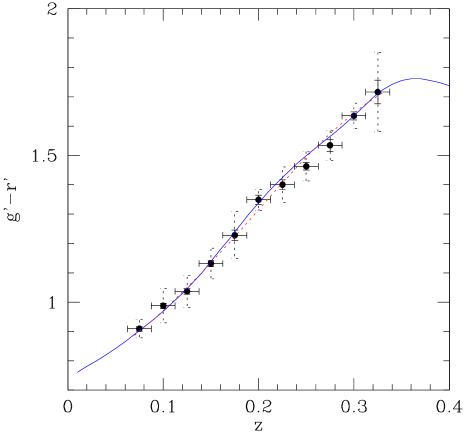
Figure 3: Observed $g^{\prime}-r^{\prime}$ color of the galaxies on the red sequence as a function of z. Dotted error bars in the ordinate mark the observed scatter around the median, while solid error bars mark error on the average. Error bars in the abscissa mark half the bin width. The solid curve is the expected location of an unevolving E, while the dotted line (barely different from the solid line) is an empirical interpolation. There are 15 clusters per point, on average.

Figure 2 shows the error introduced by measuring the cluster redshift using a single galaxy, by histogramming the 95 values of the individual $\Delta z$ that we computed for clusters with two or more galaxies with known redshift. The distribution peaks to $z=0.000$ (i.e. no systematics are there) and the width of the distribution is 0.0033 in $z$ (or about 1000 km s^-1). Given the observed relation between color and redshift (Figure 3, discussed later) the cluster velocity dispersion enlarges the dispersion in the rest–frame color by $0.01/\sqrt{2}$ mag, a negligible quantity.

Most importantly, only 17 % of the clusters are outliers, i.e. their $\Delta z$ is off, by more than 3 $\sigma$ (i.e. by about 0.01).

There is a second method to derive the percentage of wrong redshift assignations. In the area of best detection, there are 2726 galaxies within the 0.1 mag strip, and, statistically, only 488 (i.e. $\sim 18$%) should be background galaxies. Galaxies with redshift in the EDR–SDSS database are a subsample of the 2726 galaxies, skewed toward cluster members for two reasons. First of all, the main EDR–SDSS survey targets only bright ($r^{\prime}\raisebox{-2.15277pt}{$\,\stackrel{{\scriptstyle<}}{{\scriptstyle\sim}}\,$}17.77$ mag) galaxies, while the number computed thus far are for $r^{\prime}<21.0$ mag. At bright magnitudes the cluster contrast with respect to the background is higher, by a factor of several, than over the whole studied magnitude range. Hence, the contamination is likely 5 to 10 %, or less. Second, fainter galaxies with measured redshift belong to the “Luminous Red Galaxy” sample, that targets the most luminous and red galaxies in the Universe, common in clusters and rare in the field. This selection further reduces the expected contamination. A posteriori, only few red sequences are much redder or bluer than the average, implying that wrong cluster assignations are rare, as we will show in section 3.1 by a third method.

To conclude, one redshift is enough to determine the cluster redshift if it comes from a red sequence galaxy, 90 % of times. Robust statistics, that we adopt, overcomes the effect of a few mis–assigned redshifts. On the other end, we cannot firmly exclude the existence of very rare clusters whose red sequence has a color very different from the remain of the sample.

To summarize, the two drawbacks of assumption n. 2 have a negligible impact or concern a minority of clusters, and the latter can be deal with by using robust statistics.

Out of 634 clusters, 158 have a known redshift in the range $0.06<z<0.34$. In the photometric redshift range $0.06<z<0.30$, where photometric redshifts are accurate (see Sect. 3.7), there are 370 clusters, of which 127 have a known redshift. Therefore, the studied sample is about one third of the clusters detected in the EDR–SDSS, in the same redshift range.

One more technical detail should be now mentioned: when a cluster has $n>1$ galaxies with redshift, approximations 1) and 2) need one more specification: which one, among the galaxies with redshift, is the galaxy that defines the color and redshift of the cluster. The analysis presented in this paper is performed in two different cases: a) taking the galaxy nearest to the cluster center or b) taking all the galaxies, i.e. duplicating the cluster $n$ times, once per galaxy with $z$. Since the results are independent on such an assumption, we quote only results for case b).

2.3 Color biases induced by spectroscopy

The EDR–SDSS catalog includes a galaxy spectroscopic sample composed by two subsamples. A first one is an usual flux–limited sample ($r^{\prime}\raisebox{-2.15277pt}{$\,\stackrel{{\scriptstyle<}}{{\scriptstyle\sim}}\,$}17.77$) mag (Strauss et al. 2002). The second one, the “Luminous Red Galaxy” (Eisenstein et al. 2001) sample is aimed to get redshifts for an absolute magnitude limited sample of intrinsically red galaxies. Therefore, the sample of galaxies in the spectroscopic database has a characteristic feature: at $z<0.2$ the galaxy luminosity function is sampled with variable depth, from $M_{r}\sim-21$ mag to $M_{r}\sim-23$ mag. At $z>0.25$ the “Luminous Red Galaxy” sample dominates, the limiting magnitude does not longer increases, and only galaxies brighter than $M_{r}\sim-22.5-23.0$ mag are included. These features are shared by the subsample of the EDR–SDSS spectroscopic database that we consider in the following.

At $z<0.25$ there is no relationship between the color of the galaxies on the red sequence and their presence in the spectroscopic database, simply because the color of the galaxies in the main spectroscopic sample are not used for the spectroscopic selection. Therefore, the subsample of clusters having redshift drawn from the main spectroscopic sample is a random (and representative) subsample of the whole sample of clusters listed in the original cluster catalog. Neither the average nor the scatter of the color of red sequence are hence affected by selection effects induced by the requirement that the cluster redshift should be known. The same should be verified to hold too for the high redshift ($z>0.25$) subsample, which is, instead, color selected, because the “Luminous Red Galaxy” sample put fibers preferentially on red galaxies, hence potentially excluding a priori clusters with a blue red sequence, if they exist. The possible lack of clusters in one tail of the distribution (the blue side) could hence reduce the observed scatter and introduce a systematic bias between the observed average colors and the true average color. However, Eisenstein et al. (2001) show that the density of the Red Luminous Galaxies is constant up to $z=0.35$. Their Figure 3 shows that the cuts used for the target selection is about 0.23 mag away from the expected color of Es (please note that the track shown in their Figure 3 is made bluer by 0.08 mag, as explained in their Appendix 2), and hence the selection only affects galaxies too blue to be of interest here. Therefore, at the largest studied $z$ too, the target selection is color–independent for red sequence galaxies, and both the average color and the scatter are safe.

3 Results

3.1 Main trend

Figure 3 shows the $g^{\prime}-r^{\prime}$ color as a function of redshift, for $0.06<z<0.34$. At each redshift a finite and small dispersion is found (dashed error bars). Furthermore, there is a clear trend for redder colors at high redshift, as expected, due to the differential k-corrections between the two filters. Therefore, any measure of the color dispersion should be reduced to the rest–frame.

Figure 3 shows also errors on the mean color at each redshift (small solid error bars) and the expected track of an unevolved (spectro–photometric) elliptical (continuous line). The error on the mean (median) is assumed to be equal to the dispersion divided by $\sqrt{N*0.8}$ in order to approximately take into account the presence of outliers and the reduced efficiency of the median with respect to the mean. The track has been computed by using the elliptical spectrum listed in Coleman, Wu & Weedman (1980), adopting the filter response of EDR–SDSS filters, convolved with the CCD quantum efficiency and atmosphere transmission, as listed in the EDR–SDSS web page. The rest–frame color of ellipticals is taken to be $g^{\prime}-r^{\prime}=0.74$ mag, (Frei & Gunn 1994). Our k–corrections are almost identical to those listed in Frei & Gunn (1994) and Fukugita, Shimasaku, & Ichikawa (1995), but we have a dense sampling in $z$, absent in the cited papers. The continuous line is not a fit to the data, being no free parameters. Qualitatively, the agreement is very good: the observed color change is the one expected assuming no evolution and an elliptical spectrum for red sequence galaxies. The agreement is even surprising, considering the claim that there are residual (admittedly small) errors in the precise photometric calibration of the EDR–SDSS data (Stoughton et al. 2002). Given the observed agreement between observed and expected colors, residual calibration errors should almost cancel out in the $g^{\prime}-r^{\prime}$ aperture color.

The agreement between the observed color and the non–evolving E track is expected, because the passive evolving track (computed by using Bruzual & Charlot (1993) models), and the not–evolving track are expected to be almost identical (passive evolution accounts for $\sim 0.02$ mag of blueing at $z=0.25$).

The dotted line shows an empirical interpolation, as provided by an artificial neural network trained on the individual $(z,g^{\prime}-r^{\prime})$ pairs. The two curves are identical, showing that in order to derive the scatter around the track it makes no difference to assume a model for the redshift dependence of $g^{\prime}-r^{\prime}$ color or to empirically derive the latter directly from the data themselves.

The median absolute difference between the track and the points is 0.01 mag, and therefore the track is an accurate description of the data. According the $\chi^{2}$ test, the E track is an acceptable description for the blueing of the red sequence, since the reduced $\chi^{2}$ is $\chi_{\nu}^{2}=1.68$ for 11 degree of freedom, and the track can be rejected at the 90–95 % confidence level only.

There are small deviations from the track and sophisticate statistical tests that use the individual 253 data points and that look for correlated deviations from the track in localized redshift ranges (focus your attention, for example, on the three points below the track at $z\sim 0.25$, each one being the median of about 20 individual data points) can reject the track as acceptable description of the underlining individual data points at a large confidence level. There are two reasons for expecting these (admittedly small) deviations. First of all, the track gives the expected color of an elliptical galaxy of a fixed absolute magnitude. In our sample, instead, the absolute magnitude admits all values that allow the galaxies to be included in the spectroscopic sample. The average absolute magnitude of galaxies in the spectroscopic database depends on redshift, because the spectroscopic sample is largely a flux limited sample (Section 2.3). Because of the color–magnitude relation, at large redshifts the sample is dominated by brighter and therefore redder than average early–type galaxies, while at low redshifts the sample is dominated by fainter and therefore bluer than average early–type galaxies. Second, colors are measured in a fixed aperture in the observer frame (a 3 arcsec aperture), not in a fixed aperture in the galaxy frame as implicitly assumed in the computation of the track. Because of existence of color gradients in early–type galaxies and the use of a fixed aperture in the observer frame, distant galaxies appear bluer (because aperture is larger in their rest–frame), than nearby ones, all the remaining kept fixed.

Therefore, the color of the objects should be reduced to a fixed absolute magnitude, by adopting a slope for the color–magnitude relation and a correction for the color gradients inside the galaxies. Both these informations (slope of the color–magnitude relation, amplitude of the color gradients, and eventually their dependence on the absolute magnitude) are unknown at the present time for the EDR–SDSS photometric system. We can, however, take an empirical approach, by reducing the color of the galaxies to those of $M_{r}=-22.5$ mag galaxies by adopting a correction that is similar to the color–magnitude relation:

$(g^{\prime}-r^{\prime})_{corr}=(g^{\prime}-r^{\prime})+\alpha(M_{r}+22.5)$

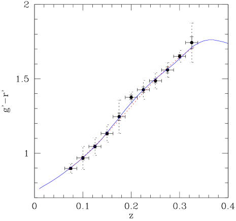
Figure 4: Observed $g^{\prime}-r^{\prime}$ color, corrected for the color–magnitude relation and the color gradients inside galaxies, of the galaxies on the red sequence as a function of $z$. Error bars and curves are as in Figure 2.

where $\alpha$ is a parameter to be determined from the observations, and $M_{r}$ is the absolute magnitude of the considered galaxy. Adopting $\alpha=-0.02$, we are able to remove the dependence of color residuals from redshift, dependence pointed out by correlated deviations from the track in localized redshift ranges. This correction is of the order of 0.01 mag. Figure 4 shows the corrected $g^{\prime}-r^{\prime}$ color, as a function of redshift.

Since the average color of the red sequence is well described by our synthetic track, at the 0.01 mag (median absolute deviation between the track and the data points), and residuals do not longer correlate with redshift, we can remove the redshift dependence of the red sequence color fairly accurately. Because of the very tiny mismatch between the data points and the track, the dispersion (robust dispersion of the absolute deviations) in color of the red sequences is inflated by 0.015 mag, but without dependence on $z$.

3.2 Scatter of red sequence

Figure 5 shows color residuals from the E track. The (robust) dispersion, i.e. the observed scatter in color of the red sequence across clusters, is 0.054 mag, as listed in Table 1. We remind that the galaxies entering in this plot (and following ones) are only those having a spectroscopic redshift (158 clusters sampled with 253 galaxies). Their absolute magnitude distribution is described in section 2.3.

We checked if part of this scatter is due to systematic effects, such as color drift across the survey. We was unable to find any trend between color residuals and observing run, CCD id, right ascension or declination, hence supporting the non–systematic nature of the scatter.

We stress here that without the color correction described in the previous section the dispersion of residuals would be even smaller (by a negligible quantity): 0.052 mag instead of 0.054 mag. Therefore, by keeping the data as they are, the data themselves point out that the intrinsic scatter of the red sequence is very small and not artificially reduced by our “corrections” (that instead make it marginally larger!).

We emphasize that the same result is obtained in two independent ways: a) by adopting the CWW spectrum and the color correction (that can be questioned) outlined in the previous section or, b), by adopting a pure empirical approach (the Neural Network interpolation), that avoid any assumption on color gradients and on the slope of the color–magnitude relation.

The use of a robust measure reduces the impact of outliers (clusters with wrong redshift assignment), that are naturally discarded. Even better, we can estimate the number of clusters with wrongly assigned redshifts, under the assumption that residuals are Gaussian distributed. In the distribution shown in Fig 5 there are 220 galaxies, out of 253, within $\pm 2\sigma$. Therefore, assuming a Gaussian distribution, 230.6 (=220/0.954) galaxies are expected in absence of wrongly assigned redshifts. We have, instead, 253 galaxies, i.e. 22 more. This difference ($\sim 10$ % of the total number of clusters) is an upper limit to wrongly assigned redshifts.

Part of the observed scatter is of observational nature, not intrinsic to variations from cluster to cluster of the color of the red sequence. There are a few major sources of scatter: first of all, Poissonian photometric errors on colors (listed in the EDR–SDSS database) account for 0.023 mag (Table 1). Second, there are further photometric errors, due, for example, to the variations of the point spread function over the EDR–SDSS camera (Gunn et al. 1998). For these errors it seems safe to assume a 0.02 mag error. Third, the E track is removed with an accuracy of 0.015 mag (Section 3.1). Finally, the velocity dispersion of galaxies in cluster induces a $0.01/\sqrt{2}$ mag term (Section 2.2). By subtracting off quadratically these four terms from the observed scatter, we found 0.041 mag (Table 1).

3.3 Redshift dependence of scatter & biases

Figure 6 shows the color residuals from the E track, after splitting the sample in near ($0.06<z<0.15$) and far ($0.15<z<0.36$). The centers of the two distributions are almost identical (Table 1), confirming the accuracy of our color corrections. The two samples have identical dispersions, 0.040 and 0.041 mag, after correction for photometric errors (see also Table 1). The two histograms computed instead without aperture and color corrections would differ by a tiny quantity, some 0.010 mag, but the large number of data points allows an F test to reject the possibility that the two distributions have the same mean at an uncomfortably high statistical level. In order not to incorrectly claim that the color of the red sequence evolves in our redshift range, color corrections must be applied. No evidence for a variation in the color dispersion is also found when color variations are removed using our Neural Network interpolation, making the found dispersion constant irrespective of any assumption on color gradients and on the slope of the color–magnitude relation.

Highest redshift bins are populated by many “Red Luminous Galaxies”. The distance between the color cut for the target selection and the E track is about five times the observed scatter in color. Therefore, the distribution of color residuals is not biased by cutting its blue tail at five sigma from the center, especially when one realizes that much less than one cluster would be removed by such a cut. Hence, the small dispersion in the higher redshift bin is not due to a selection effect (a correlation between the galaxy color and the way galaxies are selected for spectroscopic observations), confirming the conclusions presented in Sect 2.3.

3.4 Hierarchical scenario

Most of our sample is composed by low mass clusters and groups, so poor that they are not listed in the Abell (1957) catalog, not even in the $R=0$ class. In the Abell catalog there are several examples of clusters less massive than 2 $10^{13}M_{\odot}$ (see Table 3 in Girardi et al. 1998), and, therefore, there is no doubt that our sample, that contains many clusters too poor to be listed in the Abell catalog, includes the groups considered by Kauffmann (1996). Our sample also includes rich clusters, both because in our sample there are clusters listed in Abell (1957) with $R>0$, and because sampling a volume larger than Abell (1957) we have rich clusters not listed by Abell because too far. Hence, our mass range is appropriate for the comparison with hierarchical models.

A solid prediction of the hierarchical scenario is that giant ellipticals in groups (defined as $10^{13}M_{\odot}$) are about 4 Gyr younger than giant ellipticals in clusters (defined as $M\geq 10^{14}M_{\odot}$). An attentive inspection of Figure 2 in Kauffmann (1996) clarifies that the claimed 4 Gyr age difference holds for the whole magnitude range studied in this paper. At the midpoint of our sample, $z=0.2$, a 4 Gyr age difference produces a 0.23 mag difference in $g^{\prime}-r^{\prime}$, adopting the same prescriptions as described in Kauffmann (1996; i.e. a 11 vs 7 Gyr GISSEL (Bruzual & Charlot 1993) template). At the highest redshift end, the difference would be even larger, because of the reduced time between the start of the star formation and the epoch (redshift) of the observed clusters.

However, the observed dispersion is 0.054 mag (Table 1), and the intrinsic scatter across clusters $\sim 0.02$ mag (see Section 3.6). No blue tail, due to groups and poor clusters, is seen, contrary to the predictions of the hierarchical model, and in good agreement with the environmental independence of the Fundamental Plane (Pahre, de Carvalho, & Djorgovski 1998; Kochanek et al. 2000). Furthermore, in the next section, we will show that the color of the red sequence does not correlate with richness, as instead the hierarchical scenario predicts.

3.5 Environmental dependence of scatter & Hierarchical scenario

Figure 7 shows the color residuals from the E track, cutting the sample inside ($R<250$ kpc) and outside ($R>250$ kpc) the cluster core. Red sequence colors outside the cluster core are bluer, on average, by 0.023 mag, and have a larger (photometrically corrected) dispersion, 0.052 vs 0.030 mag (Table 1). We interpret the bluer color and larger dispersion at larger radius as due to the morphological segregation: as the clustercentric radius increases, the fraction of spiral galaxies increases. Since spirals are bluer than early–type galaxies, the color of the red sequence become bluer and more dispersed at larger clustercentric radii, as observed in 11 clusters by Pimbblet et al. (2002). It should be mentioned here that many spiral galaxies in nearby clusters have colors similar to early–type galaxies: see, for example, the color distribution of the morphological types in Fig. 3a in Andreon (1996) for a complete sample of galaxies in Coma, or Table 2 in Oemler (1992). Therefore, many spirals can be within the color strip centered on the red sequence, but preferentially in the bluer part, hence making the average color bluer, and the dispersion larger.

The blueing of the red sequence can be, alternatively, due to an intrinsic blueing of the early–type galaxies at large clustercentric radii, as advocated by Abraham et al (1996). The issue cannot be solved with EDR–SDSS data, because the angular resolution of the imaging data is not adequate to determine morphological types with good accuracy. In fact, a good morphological classification needs the following angular resolutions: $0.06/z$ arcsec (1.9 kpc, $H_{0}=50$ km s^-1 Mpc^-1), according to Dressler (1980), 0.8 kpc (Andreon 1996 and Andreon & Davoust 1997, $H_{0}=50$ km s^-1 Mpc^-1), or even 0.65 kpc, in order to match the high resolution observations of the Hubble Space Telescope at $z\sim 0.4$ (Andreon, Davoust & Heim 1997, $H_{0}=50$ km s^-1 Mpc^-1). In angular terms, this implies sub-arcsec seeing for all clusters in our sample, i.e. a resolution outside the EDR–SDSS capabilities. In order to claim that the blueing is really intrinsic, one should also check if residual interlopers, left over after our spectroscopic selection, have a role in the observed blueing and increasing scatter at large clustercentric distances.

The found blueing is related to the proper distance (i.e. in Mpc) from the cluster center (or any quantity correlated to it, such as the local density of galaxies). In fact, if we split the sample in two parts by considering separately galaxies detected in the inner half detection area from those detected in the outer half, no differences are found in the median color or dispersion (Table 1, Figure 8). The latter splitting, while putting galaxies sitting at larger clustercentric distances preferentially in the outer sample, mixes together near and far galaxies when proper distances are adopted, because the detection area is not fixed in Mpc². In Figure 8 it could happen that a galaxy with $R<0.25$ Mpc (say) is put in the outer sample, while another one at larger radii is put in the inner sample.

Does the red sequence color depends on the cluster richness, as advocated by the hierarchical scenario? At the present time, we don’t dispose of a good (i.e. redshift invariant) measure of richness for the detected clusters, but just of the number of galaxies $N_{g}$ brighter than $r=21.5$ mag in the detection area. Depending on redshift, different portions of the luminosity function and of the cluster area (in Mpc²) are considered. Furthermore, even at a fixed redshift, a fixed detection area correspond to different cluster portions. Finally, clusters are best detected on different scales, even at a fixed redshift, making the situation even more complex. Therefore, a clean separation of rich and poor clusters (say richer and poorer than a given class) is not presently possible. We can, however, approximately split the sample in two sub–samples whose richness distributions overlap somewhat, but whose average richnesses are different. Let us consider for simplicity only clusters best detected at the smaller detection area (that are the majority), 2.5 arcmin of size. At each fixed redshift, we took a threshold that divides the sample approximately by two (high and low richnesses), thus creating two samples whose average richnesses are different on average. We call them “dense” and “loose” clusters, in order to emphasize that our richness measure is more similar to a central density than to a global richness. In practice, the observed richness, $N_{g}$, depends on redshift approximately as $(1+z)^{-1.5}$, and therefore a single cut at $11/(1+z)^{-1.5}$ galaxies inside the detection area suffices for our aims.

Figure 9 shows the color residuals for the “loose” (open points) and “dense” (close points) samples. In rich clusters the red sequence is redder, on average, than in poor clusters, by 0.015 mag (Table 1). While the difference is statistically significant (an F test rejects the hypothesis that the two distributions have the same mean at 99.99 % confidence level), the statistical difference should not be, however, overemphasized. First, the difference is tiny in absolute terms. Second, cluster samples are smaller than in the previous splitting, because we are obliged to discard clusters with best detection radii on scales different from 2.5 arcmin. Third, poor clusters have a larger fraction of spirals, and therefore are more sensible, than rich clusters, to contamination by bluer galaxies, that skews toward the blue the color of the red sequence. Fourth, poor clusters are (expected to be) smaller on average than rich ones. Therefore a fixed scale is sampling a portion of the cluster that is larger in poor clusters than in rich ones, thus again biasing toward the blue the color of the red sequence of poor clusters. On the other end, a cleaner division of clusters in rich and poor ones would probably makes the difference larger, because in this case the two classes no longer overlap.

The hierarchical scenario predicts that the brightest elliptical galaxies are 0.23 mag bluer in $g^{\prime}-r^{\prime}$ in groups than in rich clusters, a difference that it is not seen. A caveat should however be exercised: the computed hierarchical expectation assumes a metallicity independently on environment. If there is a age–metallicity conspiracy such that in low–density regions early–type galaxies are younger and also more metal-rich than in high–density environments, as suggested by some observations (Kuntschner et al. 2002), then the two effects may cancel each other in the galaxy colors. Therefore, the observed disagreement between theory and observations may be recovered if future modeling of the star formation in hierarchical scenarios will provide the required tuning between age and metallicity.

Finally, it could be argued that some clusters may be contaminated by (possibly infalling) galaxy groups or composed by filaments/superclusters seen along their major axis. This hypothetical contamination of other structures in the class of rich clusters does not help to save the hierarchical scenario, because contaminated clusters should display, in the hierarchical scenario, a color spread that is not observed.

3.6 Intercluster/intracluster scatter

The photometric–corrected observed dispersion is 0.04 mag, or less. Such a scatter is one of the smallest ever quoted, to the author best knowledge. It is composed by two parts: the intercluster scatter, related to the scatter around the color–magnitude relation, and the scatter of the color of the red sequence across clusters (intracluster scatter).

The intracluster scatter has a maximal value of 0.030 mag, as derived from the photometric–corrected observed dispersion in the cluster core (0.030 mag) assuming a minimal (zero) intercluster scatter (Table 1).

The minimal intracluster scatter can be derived assuming a maximal intercluster scatter (0.038 mag, i.e. the dispersion of an uniform deviate between -0.05 and +0.05): 0.018 mag in the whole sample and an imaginary value (but compatible with 0.000 mag) in the cluster core.

Another route is to assume for intercluster scatter the value observed by Bower, Lucey & Ellis (1992) for Coma and Virgo, 0.02 mag in $B-V$ (that approximately match $g^{\prime}-r^{\prime}$ at the median $z$ of the sample), converted from $U-V$ using Worthey (1994). Under this assumption, the intracluster scatter is 0.035 mag and 0.022 mag for the whole sample and for the cluster core, respectively, still among of the smallest ever quoted. The latter estimate assumes that poor clusters and groups have red sequences as tight as rich clusters, which is unlikely given the larger fraction of late–type galaxies in these environments, part of which fall within the $\pm 0.05$ mag color strip. Therefore, the latter two figures are upper limits to the scatter across clusters, more than measures. This conclusion is reinforced by Stanford et al. (1998) results: the intercluster scatter, 0.06 mag (derived for the $red-blue$ color), observed by Stanford et al. (1998) is systematically a bit larger than, but equal within the (larger) errors of Stanford et al. (1998), our total one, 0.042 mag (intercluster plus intracluster). The larger systematic scatter of Stanford et al. suggests that either these authors underestimate some potentially important sources of observational scatter (that should be removed from their 0.06 mag scatter), or that it exists some clusters whose red sequence is more scattered than in Coma and Virgo.

In summary, the direct measure of the maximal and minimal intracluster scatter are 0.030 mag and zero, respectively. By adopting reasonable, but unmeasured for our sample, assumptions on the intercluster scatter, the maximal intracluster scatter is $\sim 0.02$ mag.

3.7 Red sequence color as standard candle

If the color of the red sequence does not depend on redshift and environment, it can be used as a distance indicator.

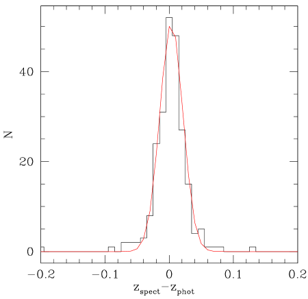
Figure 10: Residual between photometric and spectroscopic redshifts. The curve shows a Gaussian of the with of the observed distribution and of the same area.

How well can be derived the redshift from the color of the red sequence? The color of the red sequence cannot be defined for all clusters in the same way as we did for the subsample of clusters studied in this paper (that have a known redshift). We use instead the color at which the cluster is best detected. From that color we derive a $z_{photom}$ assuming the color tracks shown in Figure 4. Both the Coleman, Wu & Weedman (1980) E spectrum and a Neural Network interpolation trained on the pairs ($g^{\prime}-r^{\prime},z$) give almost identical results. The scatter between $z_{photom}$ and $z_{spect}$ turns out to be 0.018 in $z$ between $0.06<z_{photom}<0.30$, as shown in Figure 10. The considered redshift range is a bit reduced than in the remaining of the paper, because the flattening of the color–redshift relation (Figure 3) does not allow to accurately measure $z_{photom}$ at $z>0.3$. The observed scatter, computed on about 140 clusters with $z_{spect}<0.3$, is 40 % smaller than observed in Gladders & Yee (2000) at $z<0.5$ for their sample of about 20 clusters, and outperforms by a factor of 3 all photometric redshift estimates published thus far (except neural redshifts: Tagliaferri, Longo, Andreon et al. 2003a,b) and by a factor two the precision of the Fundamental Plane for a single galaxy (0.03, i.e. 15 % in $z$ at the median redshift, e.g. Jorgensen, Franx, & Kjaergaard 1996).

The greater efficiency of the red sequence color as redshift estimator with respect to photometric redshifts is likely due to the implicit selection of one single type of galaxies with a distinctive 4000 Å break (spectrophotometric bright early–type galaxies), more than the collective use of many galaxies. In fact, the same precision is achieved reducing to one the number of galaxies used per cluster (by taking the galaxy defining the color of the red sequence).

We re–emphasize here that our cluster detection algorithm is not biased against red sequence of any given color, and the low scatter found is not due to having discarded in the detection phase clusters that have a red sequence with a color different from the average. Therefore, the good agreement between $z_{spect}$ and $z_{photom}$ is not the result of having discarded (undetected) clusters for which such relation does not hold. We remind, however, that clusters with a flat color distribution, if they exist, are under–represented in our sample, because their detection probability is lower than the one for clusters with a peaked color distribution.

The color–redshift relation used to derive redshift from color is purely empirical, especially the one adopting the Neural Network interpolation. Being the relationship empirical, it is independent on the cosmological model, color corrections, galaxy evolution or k–corrections (and so on). Because empirical, the found relationship cannot be used outside the range in which it is validated (i.e. extrapolation is not allowed), and a calibration set of pairs of $(color,redshift)$ is need.

4 Summary of the observational results and discussion of the observational results

We studied the color of the red sequence of 158 clusters detected by our cluster detection method. They are the clusters with available $z$ in the spectroscopic EDR–SDSS database (in the sense explained in section 2). All along the paper we show that there is no reason why the subsample of studied clusters should be different in their color properties from the larger sample of clusters detected in the EDR–SDSS in the same redshift range. Therefore, our sample of 158 clusters is representative of the whole cluster population detected on the EDR–SDSS and in the $0.06<z<0.34$ range bare for clusters so rare that their inclusion in our sample is unlikely. Our results are therefore general because based on a large sample, and because based on a random subsample of a $\sim 4$ times larger sample of clusters.

All cluster redshifts are based on one single redshift measure. The impact of wrong redshift assignations (due to interlopers) is reduced by adopting robust statistics, much less sensible to outliers than the usual mean and standard deviation.

The average color of the red sequence changes, as a function of redshift, as expected for a red sequence populated by not evolving ellipticals with the spectrum listed in Coleman, Wu & Weedman (1980). However, the leverage given by the studied redshift range is small for discriminating plausible evolutions, such as a no–evolution from a passive one.

The total measured scatter in color of the red sequences is 0.054 mag. A virtually identical result is found without any correction for aperture and luminosity effects. Therefore, the homogeneity across clusters of the color of the red sequence is intrinsic to the data, not produced by some sly operations performed on data. We emphasize that the same result is obtained adopting the CWW spectrum plus color corrections or a pure empirical approach (the Neural Network interpolation), that avoid any assumption on color gradients and on the slope of the color–magnitude relation.

Clusters detected by our method with a red sequence bluer than the color of an E (in their rest frame) are not discarded ab initio, but are detected, if they exist. Figure 6 shows the rarity of such a type of clusters.

The overall picture is the one of extreme similarity in the color of red sequence galaxies, across clusters, and from rich clusters to groups. In itself, it is not a surprise: it is the level of uniformity and universality that stands out. It holds for an unbiased (in color) subsample of all detected clusters and groups. A hierarchical scenario would predict a 4 Gyr age difference between clusters and 10${}^{13}M_{\odot}$ groups, or a 0.23 mag color difference at the median redshift, still we don’t found any group whose red sequence is more than 0.1 mag bluer than an old elliptical galaxy. In the hierarchical scenario, the galaxy evolution should therefore pushed to high redshift, or, in alternative, high density regions could exist in a wide range of environments, and in particular, in the seeds of present day groups. One more possibility is that metallicity differences compensate age differences.

The level of the color uniformity is also outstanding: the observed scatter, inclusive of observational errors, is about 0.05 mag, the precise value depending on which sample is considered (see Table 1). Once observational effects are removed the scatter drops to 0.04 mag. If only galaxies in the cluster core are considered, the observed scatter of the color of the red sequence is even smaller, 0.03 mag (observational–corrected), suggesting that the galaxies in the cluster core are less scattered around the color–magnitude relation than galaxies at larger clustercentric radii, probably due to the lower fraction of late type galaxies that reside in the cluster core.

The color of red sequence measured outside the cluster core is bluer by 0.023 mag, and have a larger dispersion, by 0.022 mag. We interpret these differences as due to (red) spirals, whose abundance, relative to early–type galaxies, increases with clustercentric distance. However, the effect can be alternative interpreted as genuinely related to early–type galaxies, although indirect observations disfavor such possibility. Sub–arcsec resolution images are need for definitively discriminate between the two possibilities.

If clusters are divided in “dense” and “loose” with a “fuzzy” splitting that produces two samples of different average richnesses, but with the two classes overlapping somewhat, then loose clusters have marginally bluer red sequences, and we ascribe the effect to the increased spiral contamination in these clusters, with the same caveat as before.

The direct measure of the maximal and minimal intracluster scatter are 0.030 mag and zero, respectively. By adopting reasonable, but unmeasured for our sample, assumptions on the intercluster scatter, the maximal intracluster scatter is 0.022 mag.

A few caveats should be emphasized, before to proceed to a quantitative interpretation of the observational result via some model assumptions.

First: by examining the color distribution, after removal of outliers, we are describing the average properties of the red sequence of clusters. The evidence of a similarity in color for most of the sample does not exclude that very few clusters had different star formation histories, for example forming stars later/former than the bulk of the clusters. Figure 5 shows that if these clusters exists they are very rare.

Second: we found an homogeneity in color over the whole sampled redshift range. However, because of the way the EDR–SDSS spectroscopic sample is built, we are measuring the color dispersion for galaxies in a large (small) magnitude range at low (high) redshift as explained in section 2.3. Our conclusions cannot be, therefore, extrapolated to faint galaxies in the highest redshift bins, because they are not in the sample.

5 Modeling

We adopt a simple model to constrain the star formation history of the galaxies on the red sequence via their color homogeneity across clusters. The idea is to see what constrains on the synchronicity or stochasticity of cluster formation are compatible with the small dispersion (about 0.02 mag intrinsic) of red sequence colors. A successful model should produce red sequences with the observed scatter. We inspired ourselves to Bower, Lucey & Ellis (1992 and following works): via a stellar population synthesis model we infer the mean age of the last episode of star–formation and its scatter by requiring than the expected color dispersion across clusters matched the observed one. As claimed a few times in literature, the color evolution is high sensitive to systematic uncertainties of the stellar population synthesis model, and hence we prefer to rely only on differential measure only, i.e. on the scatter in color. In our specific case, systematic errors in the model (Worthey 1992) are larger than the color differences expected for reasonable choices of the scenarios of star formation.

We suppose that the red sequence evolves with a star formation rate (SFR) exponentially declining (with $\tau=1$ Gyr, a Salpeter Initial Mass Function and a solar metallicity). Early–type (passive evolving) galaxies have been thus far modeled in different ways: with a burst of star formation (e.g. Kodama, Arimoto, Barger & Aragon–Salamanca 1998), with an exponentially declining SFR (e.g. Bruzual & Charlot 1993), with an exponentially declining SFR followed by a truncation (e.g. Bower, Kodama & Terlevich 1998), or by a single stellar population (van Dokkum & Franx 2001). Depending to the reader’ preferred way to model passive evolving galaxies, our choice of SFR can be the one appropriate for a monolithic star formation scenario, or can account for fresh star formation due to galaxy infall in the cluster or residual star formation in galaxies on the red sequence. More in general, we are not assuming a monolithic formation scenario for red sequence galaxies: the exponential decay is simply intended to characterize the change of the overall rate of star formation, independently on the fact that galaxies are split between several subunits or are single–body objects, and that there is, or not, an infall in the cluster.

If we allow an important secondary infall or a more various star formation history for the red sequence galaxies, then the constrains we can put on the last episode of star formation history would be tighter than the one measured. In fact, any freedom on the evolutionary path increases, not decreases, the expected dispersion in color, unless some fine tuning is at work. Hence, in order to keep the color dispersion as small as the observed one, we should force an higher degree of coordination in the formation of the objects that we now observe on the red sequence, and/or move the last episode of star formation in the galaxy far past. It should also be emphasized that we are modeling the average evolution of galaxies on the red sequence, not the evolution of any individual galaxy. Because of the average, the evolution of the ensemble is surely smoother than the evolution of one single object, hence supporting our choice of a simple evolutionary model.

In a given cluster, all galaxies that are now on the red sequence begin their star formation all at the same time. The rationale behind this choice is that we have observationally separated the color spread inside each cluster (due to an age/metallicity spread) from the color scatter across clusters. The latter is interpreted as an age spread. The alternative, that the color scatter across clusters is given by a variation in metallicity from cluster to cluster, is interesting, but outside the aim of this paper.

While all galaxies (or subunits) inside each cluster begin to form stars at the same time, $t_{start}$, such a time differs from cluster to cluster. Therefore, each cluster has its own $t_{start}$. The $z$ distribution of $t_{start}$ is assumed to be uniform between $z_{start}$ and $z_{end}$. $z_{start}$ and $z_{end}$ are the redshift (ages) of the oldest and youngest clusters respectively. More complicate distributions can be chosen, but we anticipate that $z_{end}$ is the most important parameter, and that what happens at earlier times is largely unconstraint. Therefore, there is no need for any supplementary unconstraint parameter.

The distribution of formation redshifts, in spite of his simplicity, can capture many different global star formation rates: the only common behavior shared by the different global SFR is that at $z<z_{end}$ the SFR decrease almost linearly (in logarithmic units) with $z$.

In order to understand our sensitivity to the library used for the stellar population templates, we adopted both the GISSEL98 (Bruzual & Charlot 1993) and Poggianti (1997) libraries. Since almost identical results are found, we present results for GISSEL library only, that is sampled with a finer time resolution, and hence need only smaller interpolations between ages. In order to check our code, we verify that K and E corrections (whose moments are at the base of our computations) computed by us are identical to the values listed by Poggianti (1997) for the same library and filters (we use Johnson filters in the comparison, for lack of SDSS filters in the Poggianti’ set).

In practice, we generate 1000 objects, each one representing the average of all galaxies on the red sequence of an individual cluster, with the appropriate $t_{start}$ distribution, and we left the objects to evolve toward the observed redshift, $z_{obs}$, assuming an exponentially decreasing star formation history. Then, we (synthetically) observed them through the EDR–SDSS $g^{\prime}$ and $r^{\prime}$ filters including the effect of CCD quantum efficiency, telescope and atmosphere transmission and we compute their scatter in color at $z_{obs}=0.1$ and $z_{obs}=0.25$. These two redshifts are the midpoints of the two redshift ranges studied in the previous sections. Results at $z=0.1$ hold for the color of red sequence, as measured over a 3-4 mag magnitude range, while results at $z=0.25$ hold only for the brightest galaxies. Such a choice is dictated by the limitations of the used observational data set: we never measured the color of distant and intrinsically faint galaxies simply because they are not spectroscopic targets of the EDR–SDSS.

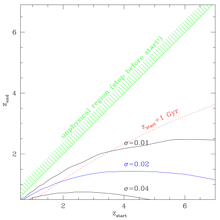
Figure 11: Constrains on the star formation history of galaxies on the red sequence at $z=0.1$, for three values of the intracluster color dispersion: 0.04, 0.02, and 0.01 mag. The dotted line marks the redshift at which the universe is 1 Gyr older that at $z_{start}$.

Figure 11 shows the constrains we can put on the star formation histories from the scatter of the color of red sequences at $z=0.1$. In this figure, as well as in the next one, only half of the region is permitted, because the star formation cannot stop before to start. The dotted line marks the redshift at which the universe is 1 Gyr older that at $z_{start}$. The elapsed time between $z_{start}$ and $z_{end}$ is less than 1 Gyr for points above the curve. An observed intrinsic dispersion of 0.02 mag (middle curve) can be produced by several pairs of $z_{start}$ and $z_{end}$. If stars in the oldest clusters formed at $z>2$, i.e. $z_{start}>2$, then the stars in the youngest clusters formed at $1.1<z_{end}<1.4$, a very precisely determined time for the age of stars in the youngest clusters (there is about 1 Gyr between $z=1.1$ and $z=1.4$). If the star formation epoch of the oldest clusters starts at smaller redshift, say $z_{start}=1$, then the start of the star formation in all the other clusters should immediately follow, implying an extreme coordination in the star formation histories of galaxies far apart in the universe and sitting in different environments (from rich clusters to poor groups), a coordination that the hierarchical scenario seems not to allow. If the maximal delay between the begin of the star formation in massive halos (clusters) and smaller ones (groups) is 1 Gyr, i.e. 1/4 of the time delay claimed to be by hierarchical scenarios, then the youngest clusters should form their stars at $z_{end}>1$, and this holds both for clusters and groups.

While the observed small scatter in color does not exclude by itself that stars in red sequences galaxies formed at $z<1$ with extreme coordination, this model is at strong discrepancy of the mere existence of galaxies at $z=3$ (e.g. Shapley et al. 2001) that are not allowed if $z_{start}<3$, unless star formation is delayed in clusters, contrary to what hierarchical scenarios predicts. Furthermore, the model colors would be too blue to accommodate red sequence galaxies in the redshift range $0.3<z<0.9$ observed by Stanford, Eisenhardt & Dickinson (1998). Therefore, in order to keep the dispersion at the observed value and, at the same time, not to contradict the mere existence of high redshift galaxies, we should discard the possibility of a late and extremely well synchronized star formation, and keep only the remaining possibility: the latest star bust episode in red sequence galaxies happens at $z\sim 1.1-1.4$. Given the fact that the 0.02 mag dispersion in color is probably an upper limits, then the $z\sim 1.1-1.4$ constrain is an lower limit.

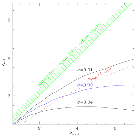
Figure 12: As previous figure, but for $z\sim 0.25$ galaxies.

Figure 12 shows the constrain allowed by the color scatter of the red sequence at $z=0.25$. With respect to the previous Figure, curves move up, showing that the coordination is tighter. We are able to put stronger constrains for two reasons: because we observed earlier in time, where galaxies were younger and color differences had less time to dump out and because we are observing a bluer part of the galaxy spectrum, part that is more sensitive to star formation episodes. Star formation stops at $z\sim 2-2.5$, almost independently on $z_{start}$, unless the star formation across all structures (clusters and groups) is synchronized at better than 1 Gyr. Again, red sequence colors at high redshift and the existence of galaxies (i.e. star) at high redshift ($z=3$ at least), both reject the low redshift part of the curve, as for the previous figure.

Both Figure 11 and 12 shows other two curves: for an intrinsic scatter of 0.04 mag, ruled out by observations, and a 0.01 mag scatter. The conclusion are qualitatively the same, but differ quantitatively. It is worth mentioning that in Figure 12 the track corresponding to an observed scatter of 0.01 mag runs almost parallel to the $z_{start}+1$ Gyr track. This means that the elapsed time between $z_{start}$ and $z_{end}$ is almost constant, independently on $z_{start}$. Therefore, if the observed scatter of bright galaxies on the red sequences is 0.01 mag, then the start of the star formation is extended and coordinated over a very short period, 0.5-0.8 Gyr only, shorter than the typical time (1 Gyr) adopted for describing the star formation in each clusters. I.e. coordination across clusters would be more precise than inside clusters.

6 Conclusions

We studied the homogeneity, across clusters, of the color of the red sequence (the intercept of the color–magnitude relation) of 158 clusters and groups detected in the Early Data Release of the Sloan Digital Sky Survey (EDR–SDSS) in the redshift range $0.06<z<0.34$. Because of the method used to detect cluster, clusters with a flat color distribution, if they exist, are under–represented in our sample.

We found a high degree of homogeneity: the color of the red sequence shows an intrinsic scatter of 0.02 mag across clusters, suggesting that either galaxies on the red sequence formed a long time ago ($z>2$) or else their star formation is universally delayed with preservation of a small spread in formation epoch. The latter possibility is ruled out by the mere existence of galaxies at high redshift. While the old age of early–type galaxies was already been claimed for a small heterogeneous collection of clusters, most of which are rich ones, we found that it holds for ten to one hundred large sample, representative of all clusters and groups detected on the EDR–SDSS. Hence we claim the possible universality of the color of the galaxies on the red sequence at $0.06<z<0.34$. Furthermore, the sample includes a large number of very poor clusters (also called groups), not studied in previous works, for which the hierarchical and monolithic scenarios of elliptical formation predict different colors for the brightest ellipticals. The observed red sequence color does not depends on cluster/group richness at a level of 0.02 mag, while a 0.23 mag effect is expected according to the hierarchical prediction. Therefore, the stellar population of red sequence galaxies is similar in clusters and groups, in spite of different halo histories. Finally, since the observed rest–frame color of the red sequence does not depend on environment and redshift, it can be used as a distance indicator, with an error $\sigma_{z}=0.018$, a few time better than the precision achieved by other photometric redshift estimates and twice better than the precision of the Fundamental Plane for a single galaxy.

The old age of stars in galaxies on the red sequence is derived by using only the color scatter, and not the color variation, the former being more robust than the latter to systematic uncertainties in the models. Furthermore, the found old age is a lower limit if there is a source of photometric errors in the EDR–SDSS not accounted for (a concern that in fact is general to all previous similar studies too). The old age of the stars in galaxies on the red sequence is in comfortable agreement with previous similar studies, such as the tightness of the fundamental plane relation for elliptical in local clusters (Renzini & Ciotti 1993), the tightness of the color–magnitude relation up to $z\sim 1$ (references listed in the Introduction), and the modest shift with redshift of the fundamental plane and color–magnitude relations (e.g. van Dokkum, Franx, Kelson, & Illingworth 1998; van Dokkum et al. 2000, Stanford et al. 1998, Treu et al. 2001). With respect to most of these studies, we used quantities less susceptible of systematic errors in the models (such as the color variation), and we consider large and controlled samples, inclusive of groups.

Table 1: The data

Sample	$\Delta$	$\sigma$	$N_{gal}$	$N_{clus}$	$\sigma_{photom}$	$\sigma_{photocorr}$
$0.06<z<0.36$	-0.001	0.054	253	158	0.023	0.041
$0.06<z<0.15$	-0.002	0.051	128	55	0.018	0.040
$0.15<z<0.36$	+0.001	0.060	125	103	0.035	0.041
$R<250$ kpc	+0.005	0.045	126	89	0.021	0.030
$R>250$ kpc	-0.018	0.063	127	69	0.024	0.052
inner half	+0.000	0.057	111	95	0.025	0.044
outer half	-0.002	0.055	142	63	0.022	0.043
half poorer, $l/2=1.25$ arcmin	+0.001	0.042	62	41	0.032	0.008
half richer, $l/2=1.25$ arcmin	+0.016	0.050	84	58	0.025	0.035

$\Delta$, $\sigma$ are the offset, relative to the E track, and the dispersion, respectively. $N_{gal}$ snd $\sigma_{photom}$ are the number of galaxies in the sample and the dispersion due to Poissonian photometric errors. $\sigma_{photocorr}$ is the scatter corrected by all photometric errors: Poissonian photometric errors, differences of the PSF in the camera, accuracy of the color trend removal, velocity dispersion of clusters.

Figure 1: Color distribution in the cluster line of sight (solid histogram) and on 100 deg² (dashed histogram), normalized to the cluster detection area.

Figure 2: Histogram of the $z$ differences for clusters having two or more galaxies with redshift.

Figure 5: Distribution of color residuals from the expected locus of an unevolving E. The curve is a Gaussian of the same median and (robust) dispersion of the data, traced to guide the eye, but never used in the paper. Error bars on data points are $\sqrt{N}$ (in the ordinate direction) and half the bin width (in the abscissa direction)

Figure 6: Distribution of color residuals from the expected locus of an unevolving E, for nearby clusters ($0.06<z<0.15$, open dots) and distant clusters ($0.15<z<0.34$, close dots). Curves and error bars as in the previous Figure.

Figure 7: Distribution of color residuals from the expected locus of an unevolving E, for galaxies inside ($R<250$ kpc, open dots) and outside ($R>250$ kpc, close dots) the cluster core. Curves and error bars as in the previous Figure.

Figure 8: Distribution of color residuals from the expected locus of an unevolving E, for galaxies in the inner half of the cluster detection area (open dots) and in the outer half detection area (close dots). Curves and error bars as in the previous Figure.

Figure 9: Distribution of color residuals from the expected locus of an unevolving E, for “dense” (solid dots) and “loose” (open dots). Curves and error bars as in the previous Figure. See text for the definition of dense and loose clusters.