Particle Splitting: A New Method for SPH Star Formation Simulations
by
Spyridon Kitsionas
A thesis submitted to the
University of Wales
for the degree of
Doctor of Philosophy
September, 2000
DECLARATION
This work has not previously been accepted in substance for any degree and is not being concurrently submitted in candidature for any degree.
Signed …………………………………. (candidate)
Date …………………………………….
STATEMENT 1
This thesis is the result of my own investigations, except where otherwise stated.
Other sources are acknowledged by footnotes giving explicit references. A bibliography is appended.
Signed …………………………………. (candidate)
Date …………………………………….
STATEMENT 2
I hereby give consent for my thesis, if accepted, to be available for photocopying and for inter-library loan, and for the title and summary to be made available to outside organisations.
Signed …………………………………. (candidate)
Date …………………………………….
Acknowledgements
I would like to thank my family for their love and support in all possible ways, during the period of my PhD studies. I still do not know how could I thank for her endless love, support and patience during the difficult three years of me living in a different country and the “strange” period of writing up. I thank my supervisor, Prof. Anthony Whitworth, for guiding me through the PhD project with his methodic work and enthusiasm. I also thank him for correcting the awful first drafts of the thesis with great patience and for making useful comments on the language and the style. I am grateful to Neil Francis for his great help.
It has been a pleasure working with Dr. D. Ward-Thompson, Dr. A.S. Bhattal, Dr. S.J. Watkins, Philip Gladwin, Seung-Hoon Cha, Glynn Hosking and Jason Kirk. I would like to make a special mention to Dr. Henri Boffin for his assistance. I thank the computing personnel of the department, Phil, Rodney and Roger, for the help, patience and skills they kindly offered me. I acknowledge the use of the Sun E4000 computer of the Cardiff Centre for Computational Science and Engineering. I also acknowledge the use of Starlink and Departmental software and equipment. I would also like to thank the head of the department, Prof. P. Blood, and my supervisor for offering me a short term research assistanceship that has been a great financial relief for me.
I thank my housemates and Simone. Living with Simone has been a great experience not just astronomically but also gastronomically! I will never forget all the friends from Italy, Spain, Germany, France, Portugal, Greece, South and Central America, India and of course Britain who have been excellent dinner, pub and party partners. I thank the five-a-side departmental team for the weekly exercise. I should also mention my friends from the BBC National Chorus of Wales as they played a special part in my social life. I thank the Akkizidis brothers and Vivian as well as Sabela and Benny for their hospitality, and my cousin for lending me her laptop.
Particle Splitting: A New Method for SPH Star Formation Simulations
Abstract
Particle Splitting is a new algorithm invented for use with self-gravitating SPH codes. It is designed to enable numerical simulations to obey the Jeans condition at all times (but it could be used in other contexts, to satisfy other conditions which require high resolution locally). With particle splitting, all coarse particles in regions of interest, are erased and replaced by sets of fine particles, increasing the numerical resolution of the simulations. A new algorithm for calculating smoothing lengths was added to our code, to accommodate the mixing of different mass particles. Our particle splitting SPH code reproduced the results of standard test simulations.
Simulations of rotating clouds with m=2 density perturbations produce a binary and a bar. We confirm that fragmentation of the bar should be attributed to inadequate resolution. By applying Particle Splitting to such simulations, we reproduce the results of high resolution finite difference simulations (Truelove et al. and Klein et al.), where bar fragmentation is absent. We obtain these results with great computational economy.
We apply Particle Splitting to simulations of clump-clump collisions. We investigate the influence of clump mass, clump velocity and collision impact parameter on the structures formed. We show that such collisions lead to the formation of shocked layers. Networks of filaments or spindles, and groups of protostellar discs form within the layers. In all collisions, fragmentation of the filaments was the common mechanism producing the groups of protostars. Low-mass secondary companions to the protostars may form subsequently by instabilities in the discs and/or dynamical interaction between the protostars. However, due to time-step requirements, we cannot follow the disc evolution for long enough to explore the formation of secondaries.
We show that all the protostars formed have mass accretion rates of 5 x 10⁻⁵ M⊙ yr-1 for the first 10-20 thousand years after their formation. This mechanism shows 10-20% Star Formation efficiency. The efficiency increases with increasing clumps mass. Collisions with impact parameter 0.4 and Mach number 10 give the highest efficiency. We predict the existence of filaments with 5 x 105 cm-3 in sites of dynamical Star Formation. These filaments could be observed in NH3 or CS line radiation, in star forming regions lying within 1 kpc.
Chapter 1 Introduction
Star Formation is a field relying on theoretical work since it is difficult to obtain observationally a picture of the way stars form. Numerical simulation of Star Formation has lately become a very popular theoretical tool due to the rapid increase in computing power. In this thesis, we deal with simulations of low-mass star formation and in particular, we establish a method for increasing the resolution and dynamic range of simulations. In this chapter, we briefly review the main theoretical and observational constraints on Star Formation, so that we can put our work in context with the other research in this field.
1.1 Stars: the end-product of Star Formation
Stars are a fundamental constituent of the Universe. Stars are hot massive dense gas spheres emitting radiation produced in their centres from nuclear reactions and/or gravitational contraction. Stars are very well studied. Analysing their spectra provides information not only on their outer layers that can be seen emitting, but also on their interiors. In particular, we can infer their chemical composition and from known nuclear reaction cycles we can produce models for their structure and time evolution. Core hydrogen burning stars of different age, mass and chemical composition define a locus on the surface-temperature vs. luminosity diagram: the Main Sequence of the Hertzsprung-Russell diagram. A star reaches the Main Sequence, following a period of gravitational contraction, as soon as the conditions at its centre become hot and dense enough to start burning hydrogen. The gravitational contraction phase of a forming star is qualitatively understood and there are theoretical models predicting its evolution towards the main-sequence (pre-main-sequence tracks). What is relatively unknown, and constitutes one of the fundamental questions for Star Formation theory, is the mechanism that brings star-forming gas together in the first place. At this point, a review of the properties of the interstellar medium, which provides the ingredients for Star Formation, can help us put this question into perspective.
1.2 Properties of the ISM
The Interstellar Medium (ISM) consists of gas in all states (atoms, molecules, ions) and dust grains. The dust component accounts only for 1-2% of the mass of the interstellar medium. The gas consists mainly of hydrogen and helium. A small percentage of the gas mass is in the form of heavier elements.
The ISM is far from being uniform, as it consists of dense clouds of gas ( cm-3). In these clouds, the gas is mainly molecular and cold ( K). Apart form H2, the clouds contain quite a few other molecules, such as CO, OH, CH, H2O, CS, NH3 as well as more massive and more complex carbon chains [\astroncitevan Dishoeck & Hogerheijde1999]. Such clouds are called Giant Molecular Clouds (GMCs) because of their size ( 10-20 pc and - M⊙). These clouds are immersed in a warm ( K) and rarefied ( cm-3) interclump medium, partly atomic and partly ionised.
The structure of the ISM is evolving with time. Parts of a GMC in proximity to massive stars can be ionised by expanding nebulae (HII regions, supernova remnants) and become part of the interclump medium, or be squashed and forced to form more stars. GMCs form in galactic spiral arms possibly through condensation of HI clouds and /or collisional agglomeration of lower mass clouds. GMCs live for about 107 yr.
GMCs are self-gravitating and they are supported by supersonic MHD turbulence. Some of the turbulent motions are generated by stars within these clouds. In particular, stellar winds and outflows, HII regions and supernova remnants are mechanisms for exciting turbulent motion. There is also evidence for magnetic fields threading the clouds (observed via polarimetry and Zeeman splitting measurements, e.g. Ward-Thompson et al. [\astronciteWard-Thompson et al.2000]).
Molecular Clouds are the birthplaces of all known young stars. They provide the initial conditions for Star Formation. “They host Young Stellar Objects (YSOs) in a wide range of evolutionary states; from Class 0 protostars some 10-2 Myr old, deriving most of their luminosity from gravitational infall, to T-Tauri stars a few Myr old, deriving their luminosity from quasi-static contraction. They also host stars in a wide range of spatial groupings; from isolated single stars as in Taurus, having no known neighbours within a few pc, to rich star clusters as in Orion, having a few thousand stars within a few pc. The masses of the stars in GMCs range from 0.1-30 M⊙, nearly the whole range of known stellar masses. Indeed the Initial Mass Function (IMF), or the distribution of stellar masses at birth, is indistinguishable between stars in molecular clouds and field stars.” [\astronciteMyers1999]
GMCs have structure of their own. Dense clumps can be observed within GMCs, typically with densities above 103 cm-3, via molecular line observations using tracers such as CO and its isotopomers. These clumps have masses between 10 and 100 M⊙. In sites of high-mass star formation, these clumps tend to be associated with groups and clusters of young stars [\astronciteLada et al.1991]. Within these clumps, dense cores can be observed using molecules such as CS and NH3 which trace densities of 104 cm-3 and above [\astronciteMyers et al.1983, \astronciteMyers & Benson1983, \astronciteMyers1983, \astronciteBenson & Myers1983]. In sites of low-mass star formation, such cores (with masses of 1 M⊙) are directly associated with the formation of single, or at the most binary, stars. It is, therefore, of great importance to understand how these cores and clumps can evolve to produce young stars. Before we list some of the available models for Star Formation, let us summarise the properties of young stars.
1.3 Observations of YSOs
Some of the cores observed in NH3 are associated with IR sources which are identified as protostars. There are also starless cores or pre-stellar cores [\astronciteWard-Thompson et al.1994], which are believed to be the precursors of protostars. They are more extended than cores containing IR sources. Some show double-peaked velocity profiles with a stronger blue-shifted peak suggesting that they are collapsing [\astronciteWard-Thompson et al.1996]. Pre-stellar cores are believed to be supported by magnetic fields. The magnetic support is removed by ambipolar diffusion [\astronciteShu et al.1987] or by reconnection of magnetic field lines [\astronciteLubow & Pringle1996]. Without this support the pre-stellar cores start collapsing.
The cores associated with IR sources also show signatures of collapse. The YSOs within these cores are not all at the same evolutionary stage. The evolution of YSOs can be divided into two major phases: the embedded phase and the revealed phase [\astronciteLada1999]. There are two different classes of objects in each phase.
In the embedded phase the protostars are collapsing fast. Their luminosity is produced by gravitational contraction and accretion. They are characterised either as Class 0 or as Class I objects depending on their Spectral Energy Distribution (SED). Class 0 objects have SEDs that can be fitted with single temperature black body functions. The Class 0 SEDs peak at sub-mm wavelengths and the objects are not observed below 20 m. Class 0 protostars are highly obscured (A 1000) and of extremely low temperature (20-30 K). Class 0 SEDs are attributable to emission from dust grains in the infalling envelope. The dust absorbs all radiation coming from the protostar and then re-emits it in the sub-mm spectral range [\astronciteAndré et al.1993]. The Class 0 phase lasts for about 1-5 x 10⁴ yr. During this period, Class 0 protostars accrete matter with a mass accretion rate of M⊙ yr-1. These objects are associated with very powerful outflows.
The SED of a Class I object is broader than a single temperature blackbody function. Class I SEDs peak at sub-mm wavelengths but they also show a characteristic excess of infrared emission. This IR emission is associated with large amounts of circumstellar dust. Class I sources are deeply embedded and there is no emission at optical wavelengths. However, there is NIR emission (e.g. 2.2 m) and a significant fraction of this NIR emission is from scattered light. Class I objects are also associated with outflows, but these are not so powerful as those of Class 0 objects. The lifetime of a Class I object is 1-5 x 10⁵ yr. During this time, the mass accretion rate is M⊙ yr-1. There is some evidence that Class I objects have come through a Class 0 phase.
In the revealed phase the protostars have evolved into pre-main sequence stars. The infalling envelope of gas and dust has been removed. The luminosity in this phase is produced by Kelvin-Helmholtz contraction and deuterium burning. Again, there are two classes of objects: Class II and Class III. Classification of pre-main-sequence stars into these two classes is based on their SEDs. The Class II SEDs are broad like those of Class I objects but they peak at IR wavelengths. For wavelengths longer than 2.2 m they decrease in a power-law fashion. The IR excess of Class II objects is smaller than that of Class I objects. Again, it indicates the presence of circumstellar dust. These YSOs can be observed in optical wavelengths, and therefore are better known than the protostars of the embedded phase. They show Hα emission which is associated with accretion onto the protostar. Optical identification of accretion discs silhouetted against a bright background has been possible with HST [\astronciteO’Dell & Wen1994]. Some of these objects have weak outflows associated with their accretion discs. Class II objects have variable emission lines; they are also known as Classical T-Tauri Stars (CTTS). From pre-main-sequence tracks, their age is estimated to be 1-4 x 10⁶ yr. Their accretion rates are estimated to be M⊙ yr-1.
During the infall of circumstellar gas onto a protostar, its angular momentum increases. Above a critical value, the excess in angular momentum, produced by more infalling mass, has to be removed. The discs provide a natural mechanism for angular momentum removal [\astronciteLynden-Bell & Pringle1974]. Mass is accumulated on the plane perpendicular to the angular momentum vector and angular momentum is transfered to the mass at the outer edge of this disc.
Class III objects are visible at both optical and IR wavelengths. Their SEDs can be fitted with single temperature black body functions. At wavelengths longer than 2.2 m their emission decreases more steeply than that of Class II objects. They show no excess IR emission. Their SEDs are thought to be arising directly from their photospheres. However, there is still considerable amount of dust around these objects (remnant of the infalling envelope of previous protostellar phases) which produces a substantial extinction and reddening. These objects could not be distinguished from main-sequence stars, if they were not emitting hydrogen lines and X-rays. The Hα emission is not so strong as in the Class II stage, but it indicates traces of a disc. Class III objects are also known as Weak-line T-Tauri Stars (WTTS). Their positions on the H-R diagram can be directly compared to predictions of pre-main-sequence tracks (they are positioned on top and to the right of the main-sequence). From these tracks we obtain their ages of 106 - 107 yr.
The discs around Classical T-Tauri stars are rather extended (100-1000 AU) but not very massive (0.001-0.01 M⊙). The central protostar, which has accreted most of its mass by this time, has mass 0.5-1.5 M⊙ [\astronciteBeckwith1999]. At the end of their evolution (Class III stage), pre-main-sequence stars have their discs stripped of their gaseous component. What little gas remains, together with the dust, is believed to form planetary systems [\astronciteRuden1999].
T-Tauri stars were first observed in the Taurus molecular cloud. Taurus is a low-mass Star Formation Region (SFR) on the northern sky at a distance of 140 pc. Taurus is the best example of distributed star formation, where forming stars are not part of dense groups or clusters [\astronciteGomez et al.1993, \astronciteGladwin et al.1999]. Young stars in Taurus have masses between 0.5 and 1.0 M⊙ and are in small clusters of 10 members.
The Orion molecular cloud (also on the northern sky, at a distance of 440 pc) is the most well-studied example of clustered star formation. It has been shown that in the center of Orion (close to the Trapezium OB stars) there are more than a thousand stars within one or two pc [\astronciteHillenbrand1997, \astronciteHillenbrand & Hartmann1998]. In Orion B, almost all stars (700) have formed in just 4 clusters [\astronciteLada et al.1991]. Discs around young stars in Orion (proplyds) have smaller radii than those in Taurus possibly due to photo evaporation of gas by the radiation field of the nearby massive stars [\astronciteHollenbach et al.1994]. This illustrates the strong effect that the molecular cloud environment has on Star Formation [\astronciteLada1999].
The more massive of the YSOs in Orion (M 2 M⊙) are Herbig Ae-Be stars and are the precursors of main-sequence stars of type A or earlier. These YSOs are not so well studied as T-Tauri stars because they are fewer of them and they are further away. Despite having luminosities large enough to drive stellar winds, these YSOs are highly obscured by their infalling envelopes. Like T-Tauri stars, they are associated with violent phenomena like jets and outflows [\astronciteChurchwell1999].
It has been shown that the IMF, , can be fitted with
[\astronciteMiller & Scalo1979]. This IMF extends the previous Salpeter [\astronciteSalpeter1955] IMF
to smaller and larger masses. In the low-mass range the Miller & Scalo IMF is flatter than the -2.35 power law, whereas in the high mass range it is steeper than the -2.35 power law. This IMF suggests that low-mass stars are greater in number than high-mass stars, and account for most of the mass.
The observed IMF puts a strong constraint to Star Formation theories, as these theories must predict a similar mass distribution. Another statistical constraint is set by the observed spatial distribution of stars.
It is well known that almost 50% of all solar-type main-sequence stars are part of a binary or higher multiple system [\astronciteDuquennoy & Mayor1991]. Duquennoy & Mayor have measured the distributions of periods, eccentricities and mass ratios for field binary systems. They have shown that the distribution of periods can be fitted with a Gaussian that peaks at 200 years, corresponding to a separation 30 AU. Pre-main-sequence binaries are observed in the same range of separations as field star binaries (from a few to 104 AU, e.g. Ghez et al. [\astronciteGhez et al.1997]). Their distribution of separations is similar to that of the field stars (e.g. Prosser et al. [\astronciteProsser et al.1994]). This indicates that stars often form in binaries.
The binary frequency may depend on the environment of the SFR [\astronciteBrandner & Khler1998]. It appears that closer binaries are formed in regions near massive stars. However, there is evidence that universal processes determine the multiplicity of young stars, since the surface density of companions for pre-main-sequence stars can be fitted with a single power law, for 0.0001, in many different regions, e.g. Chamaeleon I, Taurus, Orion, Ophiuchus, Lupus, Vela (Larson [\astronciteLarson1995]; Simon [\astronciteSimon1997]; Nakajima et al. [\astronciteNakajima et al.1998]; for a review see Gladwin et al. [\astronciteGladwin et al.1999]).
We have seen that protostars, which are very young but not very bright sources, are heavily obscured by circumstellar material for a significant period of their formation. It is, therefore, rather difficult to obtain detailed observational information for the physical mechanisms that convert the ISM into stars. Theoretical work therefore has an important role to play in Star Formation research. Modelling the complex gas dynamics in the ISM, including several orders of magnitude change in density and linear scale, is achieved by means of numerical simulations. In this thesis, we model cloud-cloud collisions. In the next section, we review the most important theories of Star Formation and previous cloud-cloud collision simulations.
1.4 Theories and Simulations of Star Formation
“Every piece, or part, of the whole of nature is always merely an approximation to the complete truth, or the complete truth so far as we know it. In fact, everything we know is only some kind of approximation, because we know that we do not know all the laws as yet. Therefore, things must be learned only to be unlearned again or, more likely, to be corrected.” [\astronciteFeynman1995].
Star Formation theories should predict the formation of groups of protostars with the above distributions of masses and separations. One of the oldest mechanisms proposed for the production of binary stars was fission, the splitting of a single object into two due to excess rotation. However, both finite difference and SPH simulations of Durisen et al. [\astronciteDurisen et al.1986] have shown that spiral arms remove angular momentum efficiently from the rotating object, and fission does not occur.
Capture predicts that an initially unbound system of two or more protostars will become bound when it loses energy in a close encounter. Star-disc capture [\astronciteHall et al.1996, \astronciteBoffin et al.1998] is a mechanism sufficient to reproduce the binary frequency in very small dense stellar clusters, but not in larger looser clusters or the field [\astronciteClarke & Pringle1991].
The well known model of low-mass star formation of Shu, Adams & Lizano [\astronciteShu et al.1987] involves the collapse of an isothermal sphere producing a single protostar. The isothermal sphere loses its magnetic support via ambipolar diffusion, where neutrals slowly decouple from the ions and the field to produce a density profile. Collapse of a sphere with such a profile gives a constant accretion rate. However, Whitworth et al. [\astronciteWhitworth et al.1996] have argued that such a profile is unlikely to arise in nature. In addition, Class 0 protostars are observed to be undergoing collapse with a less centrally condensed profile [\astronciteWard-Thompson et al.1994].
Fragmentation is a process where separate parts of a cloud, clump or core become gravitationally unstable and contract. Groups of protostars are usually produced by this process. Fragmentation requires a mechanism to induce gravitational instabilities. Several numerical simulations of fragmentation have been conducted involving clouds of different geometries or applying different mechanisms to produce the instabilities (for a review on fragmentation simulations see Bonnell [\astronciteBonnell1999]). Simulations of rotating spherical clouds [\astronciteBoss & Bodenheimer1979] or cylindrical clouds [\astronciteBonnell & Bastien1992, \astronciteBonnell et al.1991] produce binaries and/or bars that break up into lumps. In disc fragmentation simulations, spiral arm rotational instabilities in the rotating disc produce companions to the central objects [\astronciteBonnell1994, \astronciteBonnell & Bate1994].
Mechanisms of a dynamic nature that can induce gravitational instabilities and binary formation via fragmentation, include the creation of shock compressed layers triggered by the interaction of stellar winds with the ambient gas, or by cloud-cloud collisions.
Early simulations of cloud-cloud collisions produced coalescence of clouds [\astronciteStone1970a, \astronciteStone1970b, \astronciteGilden1984, \astronciteLattanzio et al.1985]. Fragmentation of a shocked layer produced at the interface of the collision was found in simulations with equations of state that included cooling of the shocked gas [\astronciteNagasawa & Miyama1987, \astronciteHabe & Ohta1992].
Subsequent SPH simulations of cloud-cloud collisions [\astronciteChapman et al.1992, \astroncitePongracic et al.1992, \astronciteTurner et al.1995, \astronciteWhitworth et al.1995, \astronciteBhattal et al.1998] have been able to resolve several orders of magnitude change in density and linear scale. These simulations produced large rotationally supported protostellar discs (200-4000AU) of high mass (5-60 M⊙). The simulations of Chapman et al. [\astronciteChapman et al.1992] involved higher mass clouds and produced filaments that fragmented, producing several discs. Rotational instabilities in the discs produced secondary companions to the protostars [\astronciteTurner et al.1995, \astronciteWhitworth et al.1995]. Increasing the impact parameter of the collision [\astroncitePongracic et al.1992, \astronciteBhattal et al.1998] assisted disc fragmentation as the angular momentum was increased. However, such simulations did not always obey the Jeans condition [\astronciteTruelove et al.1997, \astronciteBate & Burkert1997] and as a result they are suspect, i.e. the protostars may have formed numerically.
In this thesis, we apply a new method (particle splitting) that enables the Jeans condition to be obeyed throughout our simulations with minimum computational cost. With this method, the resolution of the simulations can be increased at certain times and places, creating simulations with increasingly fine resolution, nested inside an initial coarse simulation. We apply particle splitting to numerical simulations of cloud-cloud collisions.
1.5 Thesis plan
In chapter 2, we describe in detail the numerical code we use (Smoothed Particle Hydrodynamics with Tree-Code-Gravity). Most of the features of this code have been discussed in previous theses [\astronciteChapman1992, \astronciteTurner1993, \astronciteBhattal1996, \astronciteWatkins1996] and in Turner et al. [\astronciteTurner et al.1995], but they are presented here in detail in order to make the thesis self-contained. At the end of the chapter, we apply our code to standard tests for a self-gravitating hydrodynamical code, to demonstrate that it is appropriate for the problems we study.
In chapter 3, we present simulations of rotating clouds with an m=2 density perturbation. With these simulations, we try to reproduce previous results [\astronciteBate & Burkert1997, \astronciteTruelove et al.1997, \astronciteTruelove et al.1998, \astronciteKlein et al.1999], and we investigate the dependence of the code on numerical parameters such as the number of particles, the number of neighbours, the choice of the interpolating function, the initial spatial distribution of the particles. We consider this chapter to be an examination of the efficiency of the code when applied to more realistic problems.
In chapter 4, we describe particle splitting in detail. The method is then tested thoroughly. From the tests, it is shown that the noise introduced to the simulations when the method is applied, is not significant. We also apply particle splitting to simulations of rotating clouds with m=2 density perturbations: results of finite difference simulations are reproduced with great computational efficiency.
In chapter 5, we apply particle splitting to simulations of cloud-cloud collisions. We repeat the simulations of Bhattal et al. [\astronciteBhattal et al.1998] but now satisfying the Jeans condition. These simulations involve collisions between intermediate-mass clouds (75 M⊙). By comparing our results to those of Bhattal et al., we can estimate the efficiency of the new method and quantify its benefits. We then present simulations of low-mass clump collisions (10 M⊙) that have not been studied before. We investigate the influence of cloud mass, collision impact parameter and relative velocity on the filamentary structures formed in the shocked layers, on the protostellar discs formed within the filaments and on the Star Formation efficiency. Finally, we compare the properties of the stellar systems produced in our simulations and those obtained from observations of YSOs.
In chapter 6, we summarise our main conclusions emphasising the computational efficiency achieved with particle splitting. Finally, we make suggestions for improvements to our code as well as for further applications of particle splitting.
Appendix A gives a derivation of the Jeans criterion for fragmentation.
Chapter 2 Self-Gravitating Smoothed Particle Hydrodynamics
2.1 Self-gravitating Hydrodynamics
The gas in the interstellar medium is highly compressible. In star formation the self-gravity of the gas is also important. In order to describe the evolution of a self-gravitating, inviscid, compressible, non-magnetic fluid, we need to solve a system of four equations – the continuity equation, Euler’s equation, energy equation and equation of state [\astronciteLandau & Lifshitz1966, \astronciteShu1992] – with four unknowns, namely the velocity v, pressure , specific internal energy , and density , at each position in the fluid. It is implicit that these four quantities are also functions of time. The four equations read as follows:
-
•
Continuity equation
(2.1) where we have used the Lagrangian time-derivative and the fact that . The continuity equation expresses the conservation of mass.
-
•
Euler’s equation
(2.2) where is the self-gravitational acceleration, given by
(2.3) and is the artificial viscous acceleration (see discussion in §2.4). Euler’s equation expresses the conservation of momentum.
-
•
Energy equation and equation of state
In general, the equation for the rate of change of the specific internal energy reads
where and are the radiative heating and cooling rates per unit volume respectively. This equation expresses the conservation of energy. The pressure is then given by the ideal gas equation of state
where is the ratio of specific heats.
However, it is well established [\astronciteTohline1982] that prestellar gas at low densities ( g cm-3) is approximately isothermal at K (this is mainly due to the strong temperature sensitivity of ). At high densities ( g cm-3), the gas is approximately adiabatic. Therefore, we can reduce the system of equations we have to solve, by using a barotropic equation of state instead of the two equations involving the specific internal energy. The barotropic equation of state which we use reads
| (2.4) |
where is the isothermal sound speed of the gas at low densities and is the density above which the gas becomes adiabatic. For Eqn. 2.4 gives , while for , .
At high densities, the gas is approximated with a polytrope, having an index of 3/2 111The two rotational degrees of freedom that bring Tohline’s [\astronciteTohline1982] polytropic index to 5/2 are frozen out while the gas is below 400K [\astronciteWinkler & Newman1980]. Above this temperature, the rotational degrees of freedom are excited, and the 5/2 index switches on for one or two orders of magnitude increase in density, before dissociation happens and the gas finally becomes atomic with an index of 3/2., only for a few orders of magnitude. For further evolution toward stellar densities detailed radiation transport calculations are necessary. To-date, no simulation in the literature has advanced that far. Bate [\astronciteBate1998] has presented results approaching stellar densities, but with an approximate barotropic (piecewise polytropic) equation of state.
With our code, we do not attempt to model interactions between the gas and interstellar magnetic fields that thread molecular clouds. This would require a larger set of governing equations (e.g. see the MHD equations in Vazquez-Semadeni, Canto & Lizano [\astronciteVazquez-Semadeni et al.1998]), but more importantly it would require a two-, or possibly a three-, component fluid. Such a fluid has never been modelled with an SPH code and it is unknown what the resolution requirements for each fluid component would be. Exploring this is beyond the scope of the present thesis; and in any case, it is not clear that the magnetic fields observed in molecular clouds are sufficiently strong to greatly influence the dynamics of the cloud-cloud collisions studied in this thesis.
To solve the above system of equations, we have used the numerical method described in Turner et al. [\astronciteTurner et al.1995] with some later improvements. The method consists of two numerical techniques: SPH, which provides values for the hydrodynamical properties of the fluid (§2.3), and Tree-Code-Gravity (TCG), which provides values for the gravitational accelerations (§2.5). In this chapter, we shall describe in detail the method as well as the integration scheme with which we follow the evolution of the fluid in time (§2.8). To summarise the chapter, we will give a schematic picture of a complete cycle of the integration scheme (§2.10). Finally, we will briefly describe the performance of the numerical method when applied to some standard tests for a self-gravitating hydrodynamical code (§2.11). The novel modifications to this numerical method associated with particle splitting are developed in detail in chapter 4. Additional numerical techniques used for the purposes of special applications of this numerical method, are described in the relevant chapters, e.g. radiative cooling of shocked layers in chapter 5, sink particles in chapter 4.
2.2 Fundamentals of SPH
Smoothed Particle Hydrodynamics (SPH) [\astronciteGingold & Monaghan1977, \astronciteLucy1977], is a Lagrangian numerical method that assumes no symmetries or imposed grids. It is, therefore, very efficient in describing problems which involve complex 3-dimensional geometries. SPH represents the fluid by discrete but extended/smoothed particles (i.e. Lagrangian sample points). The particles are overlapping, so that all the physical quantities involved can be treated as continuous functions both in time and space. To implement this, a smoothing function (kernel) with compact support is used. This smoothing function describes the strength and extent of a particle’s influence. Bhattal [\astronciteBhattal1996] has shown that the M4-kernel, that has been frequently used in SPH [\astronciteMonaghan & Lattanzio1985], gives good results. The 3-D M4-kernel is a polynomial
| (2.5) |
which smoothes the mass of a particle out to two smoothing lengths. In SPH, the value of any quantity at a position r is evaluated using
| (2.6) |
where is the position, the mass and is the smoothing length of particle [\astronciteMonaghan & Lattanzio1985, \astronciteMonaghan1988, \astronciteMonaghan1992]. and are the values of and at . Note the normalising term which is introduced when we use Eqn. 2.5 for the kernel and substitute . In Eqn. 2.6 the summation is finite due to the fact that the kernel function has compact support. This implies that contributions from only a few close neighbouring particles are taken into account. The fact that the summation does not need to be over all particles greatly reduces the computational cost of all SPH calculations. The benefit of this fact must be balanced against the need to obtain accurate results. With being large enough we can reduce sampling errors. The value of is, therefore, of great importance. It is discussed in detail later in this chapter.


For example, the density at position r, is given by
| (2.7) |
The density profile of an isolated particle of unit mass and smoothing length , calculated with Eqn. 2.7, is shown on the left panel of Fig. 2.1.
The gradient of any quantity at a position r is evaluated using
| (2.8) |
where [\astronciteMonaghan & Lattanzio1985, \astronciteMonaghan1988, \astronciteMonaghan1992]. Note that in such an expression, a second order truncation error222These errors are introduced because we substitute the integral expressions with sums [\astronciteMonaghan1992]., , is introduced [\astronciteMoore1995]. For the M4-kernel, the gradient is given by
| (2.9) |
The gradient of the density is therefore given by
| (2.10) |
2.3 Basic SPH equations
Following Eqn. 2.8, the first two of the set of three hydrodynamical equations that we need to solve (namely Eqns. 2.1 & 2.2) should read as follows:
| (2.11) |
and
| (2.12) |
However, in such a case, we would have to use the value of , numerically estimated using Eqn. 2.6, which would introduce an error greater than the second order truncation error [\astronciteMoore1995]. Instead, we use a formulation that includes density in the gradient of the function. This formulation derives from the identities
and
Substituting for v and respectively, we obtain
| (2.13) |
and
| (2.14) |
| (2.15) |
and
| (2.16) |
As mentioned at the beginning of the previous section, SPH follows the evolution of the hydrodynamical properties of a fluid represented by a system of particles – sample points. These particles are allowed to move with the fluid, as they trace elements of constant mass. The particle motion will be discussed further in §2.6. A consequence of this fact is that we only need to estimate the fluid hydrodynamical properties at the particle positions, . Therefore, Eqns. 2.15 & 2.16 reduce to
| (2.17) |
and
| (2.18) |
where , and . The latter is used in order to utilise the symmetrical forms that Eqns. 2.17 & 2.18 have obtained with the use of Eqns. 2.13 & 2.14. This way we make sure that every interaction between pairs of particles is symmetric and hence we ensure that linear and angular momentum are conserved.
| (2.19) |
This formulation conserves mass very accurately because of the fact that the kernel function has compact support and it is appropriately normalised. It is therefore prefered to Eqn. 2.17. It is also simpler and faster to calculate. In our integration scheme (§2.8), we use Eqn. 2.18 to calculate the acceleration.
The equation for the rate of change of the specific internal energy can also be formulated in a symmetric form [\astronciteMonaghan1992],
However, here we are using a barotropic equation of state (Eqn. 2.4) to obtain the pressure. In our formulation, the barotropic equation of state reads as follows:
| (2.20) |
2.4 Artificial viscosity
In regions where particle streams collide interpenetration may occur. This is undesirable since colliding fluid elements should retain their relative positions; the colliding streams should be decelerated by shocks.
In order to make sure that particle interpenetration is inhibited and that we obtain well-defined (but not necessarily well-resolved) shocks, we have to include an ‘artificial viscosity’. We use the artificial viscosity described in Monaghan [\astronciteMonaghan1992]. This includes a linear bulk viscosity component that prevents interpenetration as well as a Von Neumann-Richtmeyer type viscosity component. The artificial viscous acceleration that acts on a particle is given by
| (2.21) |
where
| (2.22) |
and
| (2.23) |
while and (the average sound speed). The condition makes sure that only particles that are approaching particle will contribute to its artificial viscous acceleration. The above formula is symmetric in order to make sure that particle will in turn exert an equal and opposite artificial viscous acceleration on any of the neighbouring particles, , that are approaching.
has dimensions of velocity squared over density. The -term gives an artificial viscous acceleration similar to the hydrodynamical acceleration if sound speed squared is replaced by the product of sound speed times the relative velocity. It can treat a bulk colliding flow, but in high Mach number shocks the -term is needed, as in such cases, the relative velocity of the colliding flows is large compared to the local sound speed. and are tunable parameters and should take appropriately large values to prevent interpenetration. If then the artificial viscous acceleration is zero, particles penetrate each other and shocks cannot be modelled. If and are very large then the shock is very broad and it ends up not very well resolved; even mild sound waves are rapidly damped. We have adopted the value . It has been shown that these values give good results (§2.11.1, also Patsis (1999 private communication)).
Watkins et al. [\astronciteWatkins et al.1996] have shown that one can use the Navier-Stokes equations for viscous compressible flows to derive a viscous acceleration similar to the term, but the term is still needed to model accurately high Mach number shocks. The Navier-Stokes viscosity was derived to give a more realistic treatment of shear viscosity (e.g. in problems involving the evolution of protostellar discs). The formulation of Watkins et al. [\astronciteWatkins et al.1996] is derived from the standard SPH cross product expressions [\astronciteMonaghan1992].
2.5 Tree Code Gravity
We now have to define the term of Eqn. 2.18. In the case of point masses, the gravitational acceleration on each particle should be calculated as
| (2.24) |
where we have used units so that . However, for a large number of particles, , such a formulation becomes very expensive, as the computational cost scales as . Instead, we implement Tree-Code-Gravity (TCG) [\astronciteBarnes & Hut1986, \astronciteHernquist & Katz1989], which scales as .
With this method, a tree is constructed containing spatial information on individual particles and the centres of mass of groups of particles. This way, for distant interactions we can substitute individual particles with groups of particles. At every integration we have to construct the tree, walk up the tree to calculate the centres of mass and walk down the tree to calculate the gravitational acceleration.
For the construction of the tree, we use the whole computational domain as the rootcell, the top level of the tree. We then divide the rootcell into 8 subcells. These subcells define the first level down the tree. Each of them is subsequently divided into another 8 subcells, i.e. the next level down in the tree, etc. A cell at any level is not divided further only when it contains either a single particle or no particle at all.
If a cell contains more than one particle, its centre of mass is calculated using all its subcells in all lower levels. This way, for the rootcell we calculate the centre of mass of the whole computational domain. For each cell, we save the following information: cell centre, linear dimensions, pointers to its subcells, total mass and centre of mass, pointers to particles.
We calculate the gravitational acceleration at particle using the centre of mass of a cell unless the cell is so close that we must use its subcells instead. We apply a geometrical criterion in order to decide whether we shall use a cell or its subcells. Specifically, a cell is used if
where is the linear size of the cell under consideration, is the distance between particle and this cell and is the maximum opening angle, an accuracy parameter. If the criterion is not satisfied then the cell is ‘opened’ and its subcells are examined. If a subcell contains a single particle then a particle-particle interaction is calculated. The value of should be sufficiently small for close interactions to be calculated as particle-particle. Salmon, Warren & Winckelmans [\astronciteSalmon et al.1994] examined different values for and they determined that accurate calculations of the gravitational acceleration were obtained for . We have chosen the value of again driven by the need to balance accuracy against speed of calculation.
Therefore, the gravitational acceleration of particle is the sum of contributions from other particles and cells. For a particle-particle interaction with particle we use
| (2.25) |
with the potential energy given by
| (2.26) |
For the interaction with cell we write [\astronciteGoldstein1980]
| (2.27) |
and
| (2.28) |
Here is the traceless quadrupole tensor about the centre of mass. It is defined as [\astronciteGoldstein1980]
| (2.29) |
where run from 1 to 3 for each direction in Euclidean space and is the Kronecker delta, e.g. and , etc.
The quadrupole moment of a cell in the tree is based on the quadrupole moments of its subcells:
| (2.30) |
where are now the coordinates of the subcells in the reference frame of the parent cell.
With SPH we try to describe all quantities involved as continuous functions both in space and time. Therefore, we have to reduce the magnitude of close particle interactions in order to avoid unduly large gravitational accelerations (). The particles are smoothed similarly to the way they are treated for hydrodynamics, i.e. as spherically symmetric and finite in extent with a radius of . If two particles overlap, the mass involved in the calculation of the mutual gravitational acceleration is calculated from Gauss’ gravitational theorem, otherwise the particles are treated as point masses.
For particle the mass interior to radius is given by using and hence
If particle is less than away from particle then the gravitational acceleration at particle will be
| (2.31) |
which means that the mass of particle outside is not being taken into account. With this symmetric description of the gravitational interaction between particles and , we do not have to specify to which of the two particles we have applied Gauss’ gravitational theorem. Then the total gravitational acceleration at particle is
| (2.32) |
The potential at distance away from particle is then given by
Integrating by parts we obtain the expression for the mutual potential energy of two particles and :
| (2.33) |
where
For the M4-kernel we obtain
| (2.34) |
and
| (2.35) |
can take either a small constant value (- softening) which is not very good when the distance between particles changes considerably during the simulation; or it can take the value of the hydrodynamical smoothing length , which has the benefit that it smoothes the gravitational and hydrodynamical forces by the same amount [\astronciteBate & Burkert1997]. We use the latter choice, i.e. .
2.6 Smoothing length
In this section we shall discuss the importance of the hydrodynamical smoothing length, , and we shall define the range of values that it should take. SPH is a Lagrangian particle method, with the particles – sample points moving with the fluid, containing constant mass within their radius of influence. In particular, the mass of the SPH particles is considered to be smoothed over a finite volume. As mentioned in §2.2, at any time, only a few neighbouring particles overlap with the smoothing radius of any particle. Therefore, we choose the radius of influence of the smoothing kernel function, , so that for any particle and at any time, it contains an approximately constant number of neighbouring particles. For this reason, we will use a time-varying non-universal , as each particle requires its own smoothing length (e.g. in a dense region a smaller is required, than in a rarefied region, in order to contain this constant number of neighbours). Nelson & Papaloizou [\astronciteNelson & Papaloizou1993, \astronciteNelson & Papaloizou1994] have shown that with adaptive the energy is conserved quite accurately.
Because we have to treat all the physical quantities involved as continuous functions both in time and space, we need to take into account a large number of interactions to reduce sampling errors. This needs to be balanced by the fact that for too big a smoothing length SPH will under-estimate the self-density of the particles and will over-smooth all the properties of the fluid. Therefore the problem of finding the correct value for is reduced to finding the right value for the number of neighbours, , for each particle. Tests on known distributions have shown that neighbours within gives good results with the 3-D M4-kernel.
We allow a 10% fluctuation in the value of the number of neighbours, , for each particle at any time. Thus, we allow to be between and . If is the number of neighbours of particle at time-step , then a trial value for at time-step () is obtained by its value at the th time-step according to
| (2.36) |
We then count the number of neighbours within , . If is within the above limits then the value of is accepted. However, if the value of is not within the limits, we iterate over Eqn. 2.36, finding a new trial value for using , obtaining a new number of neighbours according to this new trial value of , and so on. We stop when is acceptable or when the fractional change of two successive trial values for becomes less than 1%. After we have obtained the values for all particles, we substitute these values to the current value of . To set the initial values of for all particles, we repeat the above procedure until either all particles have acceptable value for , or we exceed a finite number of iterations. Numerical tests indicate that after 20 iterations most particles have an acceptable .


We will now discuss the way we identify neighbours. A direct search would be an procedure, but using the spatial information stored in the gravity tree we can speed it up considerably. The original idea [\astronciteHernquist & Katz1989] for looking up in the tree for neighbours involved constructing a trial cube of side for particle and then identifying which cells this cube overlaps, always starting with the rootcell. If these cells contain subcells they are then examined in a hierarchical fashion until we open subcells containing single particles. We then compare the inter-particle separation with and decide accordingly.
We use a slightly modified method in order to avoid opening cells unnecessarily [\astronciteBhattal1996]. We store in the tree the values of for each particle contained in a cell. This way we can construct a bounding box, or ‘kernel box’, for each cell. This represents the minimum box that contains all the particles in the cell, when each particle is taken to extend to its smoothing radius (see Fig. 2.2). The search process is as before but with a trial cube of this time, using the kernel box for each cell instead of the cell itself. With this technique, we find all neighbours, missing no interactions within , as is the value we are actually using for our SPH equations (Eqn. 2.19 & 2.18). We only open a few cells unnecessarily and we can formulate this technique together with the calculation of the centres of mass for each cell so that we do not have to perform unnecessary walks of the tree.
2.7 SPH equations
We can now present the final forms of the three equations determining the evolution of the simulation. These are
| (2.37) |
| (2.38) |
| (2.39) |
where is given by Eqn. 2.22. For Eqn. 2.38 we have combined Eqns. 2.18, 2.21 & 2.32. , and are given by Eqns. 2.5, 2.9 & 2.34, respectively.
Parenthetically, we note that if we were solving for , the equation for the rate of change of the specific internal energy, after including heating from the artificial viscous forces, should read as
2.8 Integration scheme
We advance the positions and velocities of all particles in time using the second order Runge-Kutta integration scheme. This means that to advance particle from the th to the th step, first we need to calculate its position and velocity at the midpoint. This is given by
| (2.40) |
| (2.41) |
where is the total acceleration of particle at the th step and is the discrete time-step with which all particles will be advanced [\astroncitePress et al.1990]. We calculate from Eqn. 2.38. It is then easy to obtain the position of particle at the th step from
| (2.42) |
However, in the meantime, we must calculate the total acceleration for at the midpoint, since its velocity at the th step is given by
| (2.43) |
The selection of the time-step is of great importance. There are several time scales that can be defined locally in systems like the ones we follow. Firstly, the inverse of the local velocity divergence. Secondly, the ratio of the local length scale to the velocity at this scale. Thirdly, the square root of the ratio of the local length scale to the acceleration at this scale. And finally, a time scale similar to the second one, except that it involves the local sound speed instead of the total local velocity (separating the hydrodynamical properties of the fluid from its overall behaviour). For each particle, , we calculate the smallest of these time scales using its smoothing radius (radius of influence) as a local length scale, i.e.
| (2.44) |
where
| (2.45) |
is a modified sound speed which includes the effect of artificial viscosity. is a parameter usually taken equal to 1.2. and are the viscosity parameters (§2.4). gives the largest contribution by a neighbour of particle to its viscous acceleration. The value of is usually referred to as the Courant number and is given a sufficiently small value for the simulation to be well behaved as well as to conserve the total energy. We have adopted the value of .
By choosing the smallest of these scales, we ensure that we do not evolve each particle for a time longer than any of the time scales dictated by the local dynamical/hydrodynamical properties. For the same reasons, we select the smallest of these minimum particle time scales for the value of the global time-step at any step . Formally this is given by
| (2.46) |
2.9 Multiple time-steps

If Eqn. 2.46 gives the value of the global time-step, it is obvious that there should be particles whose minimum local time scale is much larger than . This means that if we can avoid evolving these particles with the minimum global time-step but with a time-step closer to the value they require, then there is a great gain in the speed of computation. This is the basic reason why we use the method of multiple time-steps [\astronciteBhattal1996]. This method is ideal for simulations where there exist within the computational domain both dense regions (requiring small time-steps) and rarefied regions (not requiring small time-steps). The particles are assigned individual time-steps which are allowed to vary from step to step according to their need.
Taking into account the fact that at each step there are two half steps, the method creates a hierarchy of time-step bins, each containing particles that take one half step while the particles in the immediately lower bin take one full step. Therefore, the time-steps at any bin are twice as large as the ones at the immediately lower bin. The fact that the particles are not allowed to move with arbitrary time-steps but under this hierarchy of time bins, is dictated by the need to know the positions of all particles every time we calculate the accelerations and to therefore keep the system synchronised at regular intervals.
The values of the discrete times-steps used by particles in different time bins, are therefore calculated as fractions of a maximum time-step, . In particular, the time-steps can take the following values: , , , , , . We choose the total number of available time bins, , sufficiently large in order not to put any constraint on the time evolution of the simulation. Since at any time during a simulation , where is the minimum time-step from the ones used at this time (corresponding to the th time bin), we can express the current position along the largest time-step as , where . If the system is at the start of the maximum step and all particles are in-synch.
For any particle, we calculate the ideal value of its time-step, , from Eqn. 2.44. We then put this particle into the next smaller time bin, , with time-step , where is defined as
| (2.47) |
To ensure that at the end of all particles are in-synch, we have to check whether we can accept this bin, , or not. A time bin is accepted only if the time from the beginning of the period is a multiple of the time this bin represents. Otherwise we choose the immediately lower acceptable time bin. For example, for N=5 we have . If the time-step we are checking is (), we can accept it only if . Otherwise we will assign to this particle a time-step () if , or the lowest available time-step (bin ) if is odd (Fig. 2.3). With this test we ensure that a particle can move down to a lower time bin at any time, but can only move up the time ladder at times which allow the system to remain in-synch.
As mentioned above, we need the positions and velocities of all particles to calculate the acceleration of the particles in the minimum time bin. To minimise errors we must update the positions and velocities of the particles in the upper bins for the intervening times. This is achieved by extrapolating the positions and velocities of these particles. Finally, at the end of every period the system is synchronised and the particles in all time bins have their positions and velocities updated by the integration scheme.
2.10 Going through the code ‘step by step’

Fig. 2.4 shows a flow-chart of the algorithm that dictates the evolution of the fluid in time. It demonstrates the way we assemble all the previous features of the numerical method. It represents the cycle of the integration scheme, when the system advances with the time-step in the minimum time bin, .
As mentioned in §2.8, each step consists of two half steps. The first half step starts by advancing the system by . Active particles have their positions and velocities updated by the integration scheme (Eqns. 2.40 & 2.41), while all other particles have their positions and velocities updated by extrapolation. We then need to calculate the acceleration at the half time-step for the particles in the minimum time bin. We proceed as follows: we make a new tree since the particles have just moved (§2.5). Subsequently, we update the value of for the particles in the minimum time bin (§2.6). We can then calculate the hydrodynamical (§2.3), viscous (§2.4) and gravitational (§2.5) acceleration for these particles. The total acceleration at the half time-step is given by Eqn. 2.38.
We then proceed to the second half step, when tasks similar to those of the first step are performed. Specifically, the second half step starts by advancing the system by another (Eqns. 2.42 & 2.43), and thus completing a full time-step of the minimum bin . Once again, particles in the minimum time bin have their positions and velocities updated by the integration scheme (using the acceleration at the midpoint calculated during the first half step), while all other particles have their positions and velocities updated by extrapolation. We then find the active particles for the next time-step, i.e. the particles that are going to be updated by the integration scheme and therefore need their acceleration calculated. This time the active particles are not just those in the minimum time bin, but all the particles for which the total time of the simulation is a multiple of, either the whole time-step, or half the time-step of the time bin they are in. For example, for in Fig. 2.3, all the particles in the three smaller time bins are active as they start a new step, as well as the particles in the second larger time bin as they have just completed their first half step. We will then calculate the acceleration for all the active particles, following exactly the same steps as in the first half step. Finally, before starting time-step we re-distribute the particles into time bins. In order to make sure that at the end of a period the system is in-synch, we allow particles to move up the time ladder only if is a multiple of the time-step of their time bin, which in our example means the particles in the three smaller time bins. All particles that have just completed a full step are allowed to move to smaller time bins, in our example again the particles in the three smaller time bins.
Having calculated the accelerations for all the active particles, we can then proceed to the next time-step, .
2.11 Tests
We shall now describe the performance of the above numerical method on some standard tests for a self-gravitating hydrodynamical code. In particular, first we simulate the interaction of two colliding flows in order to test the efficiency of the code’s treatment to hydrodynamics. In particular, we would like to quantify the efficiency of artificial viscosity (§2.4). We then allow a uniform sphere to collapse freely to test the efficiency of the TCG method. Finally, we combine both gravity and hydrodynamics to follow the evolution of a stable isothermal sphere in order to test the overall performance of the code. For each test we compare our results with the relevant analytic or semi-analytic solutions. We conclude that our numerical method treats effectively both the gravitational and hydrodynamical properties of the fluids we are going to simulate in chapters 3 & 5.
In quantifying the results of our tests, we need to be able to associate these results only with the performance of our numerical code. In order to decrease the numerical noise input by the initial distribution of particles, we perform all tests using clouds whose particles are taken initially to be on a lattice.
2.11.1 Colliding Flows


In order to demonstrate the efficiency of the code’s treatment of hydrodynamics, we have chosen to simulate the interaction between two colliding flows instead of a Riemann shock tube. We believe that the former test is more relevant to the problems we will investigate later in this thesis, i.e. high Mach number isothermal shocks with high compression factors. The typical Riemann shock tube test only involves a compression factor of . Nevertheless, Hosking [\astronciteHosking1999] has shown that the numerical method we are using, gives very good results for the Riemann shock tube test.
Two colliding isothermal flows will produce a strong shock, provided the Mach number of the collision, , is high. If is the pre-shock velocity of each flow in the reference frame of the shock and is the isothermal sound speed, then the Mach number is given by and we obtain the post-shock velocity of each flow, , from
| (2.48) |
[\astronciteDyson & Williams1980]. From Eqn. 2.48 we obtain the value for the velocity of the shock, , with respect to the frame of the simulation, knowing the pre-shock and post-shock velocities of each flow in this frame of reference, and respectively. Specifically, because and (as ), Eqn. 2.48 gives
After some algebra we obtain
| (2.49) |
From the continuity equation we can write
where and are the pre-shock and post-shock density for each flow, respectively. Finally, we can obtain an analytic estimate for the post-shock density for each flow
| (2.50) |
The simulation involves two colliding isothermal flows (K) each of unit length in the direction of the collision. Each flow has a velocity of 1 km s-1 in this direction. The isothermal sound speed at K is km s-1. Both flows have unit pre-shock densities. There are particles in total, taken initially on a lattice. The other two dimensions have lengths of . Eqn. 2.49 gives km s-1. Therefore, the Mach number of the shock is 5.20. This is typical of the values we shall later model. Eqn. 2.50 gives a post-shock density of .
We evolve this collision with our 3-D SPH code, using periodic boundary conditions. We do not include the TCG method as it is not relevant for this test. Fig. 2.5 shows our results at the point where the rarefaction waves at the opposite ends of the tube have propagated to one tenth of the initial length for each flow. The mean value for the post-shock density, , is 26 having a 11% dispersion around the mean. The mean value for the post-shock velocity, , is 0 to the 3rd significant figure, with a dispersion of 0.19 km s-1 around the mean. The shocked layer is not broader than the analytic solution. In fact, the wings of the shocked layer are extended to less than . The layer is well resolved as its width is 20 times larger than the post-shock .
The simulation reproduces the analytic compression factor accurately. In fact, it is slightly lower than the analytic value, as some small fraction of the pre-shock kinetic energy is transformed to post-shock random velocity dispersion instead of work done in compression. However, the biggest contribution to this random velocity dispersion comes from the breaking of the symmetry of the lattice. The particles in the shocked layer are not on a lattice any more and have random motions in all 3 dimensions. The artificial viscosity is very efficient though, as at the centre of the shocked layer the random motions are damped very effectively in all directions. Very little interpenetration is observed in the layer.
We conclude that the results of this test are encouraging, and thus the choice of the values for the artificial viscosity parameters is justified. The simulation has produced a well resolved, not broad shock with a compression factor very close to the analytic value. Comparison of this test with realistic simulations will follow in chapter 5.
2.11.2 Free-Fall collapse
For the free-fall collapse simulation, we let a uniform density sphere of mass and radius collapse under its self-gravity. For this test we do not calculate the SPH equations, since the aim of this test is to verify the efficiency of the TCG method. Therefore, the acceleration in the integration scheme (§2.8) is given only by Eqn. 2.32.

The sphere should collapse homologously to a point after a free-fall time, . The analytic solution for the free-fall collapse of a uniform sphere states that any fluid element initially at radius will arrive at radius at time given by
| (2.51) |
where [\astronciteSpitzer1978]. The free-fall time for a uniform density sphere is defined as
| (2.52) |
We construct a M⊙ uniform density sphere with SPH particles on a lattice. The sphere is then let to collapse for 1 . As particles come closer due to collapse, the gravity softening is becoming smaller. However, decreases slower for the particles close to the edge of the sphere than for those at the centre. This happens because particles close to the edge can find their neighbours only from the inner side of the outer boundary of the sphere. Having a larger than they should, the gravitational acceleration for these particles is over-softened. This reduces the rate with which they collapse. To overcome this problem, and only for this test, we assign to all particles the same , the mean value of .
Fig. 2.6 compares the analytic solution (solid lines) with the values obtained from the simulations every 50 time-steps (points), for the 90%, 50% and 10% mass radii. The above edge effects, although reduced due to our treatment of , give a small over-estimation for the 90% mass radius. The inner two radii agree closely with the analytical solutions.
2.11.3 Stable Isothermal Sphere


Finally, we test both the SPH and TCG methods in evolving a stable isothermal sphere. We construct the sphere using a combination of the hydrostatic balance and mass conservation equations
| (2.53) |
with initial conditions
Using the Chandrasekhar [\astronciteChandrasekhar1939] dimensionless expression for Eqn. 2.53 we obtain
| (2.54) |
where we have substituted , and . The solution of Eqn. 2.54 formally extends to . We can truncate the sphere at a finite radius, , provided that the pressure at the boundary of the sphere is balanced by an external pressure. For the sphere is stable.
We then solve Eqn. 2.54 numerically. We tabulate the values for , and . Giving values to the total mass of the sphere , the sound speed and we can substitute back to find , and M. We have chosen M M⊙, km s-1 (corresponding to K) and .
We then move 10,000 particles taken from a uniform density lattice to reproduce the tabulated values for , and M. The solution to Eqn. 2.54 is given by the solid lines in Fig. 2.7. We have also plotted the initial radial density profile (left panel) and the radial density profile after 25 (right panel). We use crosses to present our initial data due to the fact that the initial distribution comes from a lattice and the radial profile consists of too few different points. We do not need crosses in the right panel of Fig. 2.7 as the particles have moved from their initial positions. However, the simulated radial density profile obeys the analytic solution very well. Note that at radii larger than 0.04 pc, there is an under-estimation of the density due to boundary effects similar to those described in §2.11.2. In particular, particles close to the edge of the cloud have larger than they should.
Chapter 3 Simulations of Rotating Clouds with m=2 Density Perturbations
Simulations of fragmentation are only reliable if the Jeans condition is obeyed (Truelove et al. [\astronciteTruelove et al.1997, \astronciteTruelove et al.1998], Klein et al. [\astronciteKlein et al.1999], Boss et al. [\astronciteBoss et al.2000], Bate & Burkert [\astronciteBate & Burkert1997], Whitworth [\astronciteWhitworth1998]; for a review see §4.1). In this chapter we perform the standard test simulation first proposed by Boss & Bodenheimer [\astronciteBoss & Bodenheimer1979]. We show that our SPH code faithfully reproduces the results obtained by Truelove et al. [\astronciteTruelove et al.1997, \astronciteTruelove et al.1998] using an adaptive finite difference code, and by Bate & Burkert [\astronciteBate & Burkert1997] using their SPH code (§3.2). This way, we test our code on a more realistic application and find that the results are consistent with those of Eulerian codes and other SPH codes. We also draw conclusions on the significance of the Jeans condition for fragmentation simulations. We note that the Bate & Burkert [\astronciteBate & Burkert1997] SPH code has been developed independently from our code and differs from our code in several fundamental regards.
We perform a series of simulations by changing the density above which adiabatic heating operates (§3.4.2). This way we can make a direct comparison between the results of our code and those of Bate & Burkert [\astronciteBate & Burkert1997].
We also perform a series of simulations by gradually increasing the number of neighbours as a means of testing convergence to the known solutions (§3.4). We perform both isothermal simulations and simulations which include adiabatic heating. For each case, there are 2 subsets of simulations: low resolution and high resolution, depending on the total number of particles used.
Knowing the solution to this problem, we can also explore some other numerical parameters of the code. In particular, we verify the choice of the interpolating kernel (M4) by repeating a few simulations using a different choice of kernel (§3.5). We also test whether our results are corrupted by the choice of the initial spatial distribution of particles (§3.6). But first, let us define the initial conditions for the simulations described in this chapter.
3.1 Initial Conditions
The standard test simulation for a Star Formation code is the evolution of a rotating, spherical, uniform-density, isothermal cloud with an m = 2 perturbation. The initial conditions we have used for this simulation are taken from Boss & Bodenheimer [\astronciteBoss & Bodenheimer1979]. In particular, we have constructed a uniform-density, isothermal spherical cloud of mass M = 1 M⊙ and radius R 0.02 pc. The sound speed is km s-1 (corresponding to K), which assigns to the cloud a ratio of thermal to gravitational potential energy 0.26. The spherical cloud is constructed with particles cut either from a settled uniform distribution or from a uniform face-centred cubic lattice. The particles are then given an m = 2 azimuthal perturbation with amplitude = 10, by adjusting their spherical polar azimuthal coordinate, , to a value given by
Finally, the cloud is given a uniform rotation (angular velocity = 7.2 x 10⁻¹³ rad s-1), so that the ratio of rotational energy to gravitational potential energy is 0.16. We use clouds having different numbers of particles depending on the problem. In all cases, we apply our full SPH code as given in chapter 2. When a cloud has to be evolved isothermally, we use
instead of Eqn. 2.39.
In order to decrease the numerical noise input by the initial distribution of particles, we perform most simulations using clouds whose particles are taken initially to be on a lattice. To verify that the results of such simulations are not biased due to some preferred orientation of the initial lattice, we also perform one simulation where particles are taken initially from a “settled” distribution (§3.6). Such a distribution of particles is produced when the particles are taken in random positions and then they are relaxed to uniform density, using the SPH formulation described in Whitworth et al. [\astronciteWhitworth et al.1995].
All figures presented here are column density plots viewed along the rotation axis. The geometry of the problem (fragmentation happens on a flattened disc) supports the use of such plots, since projection effects are small. It also allows comparison with density contour plots or density equatorial slices, used by other workers, as most of the mass of the system ends up in the disc. The figure captions indicate the units of the colour tables. They also give the linear size of the figure and the time of the simulation.
3.2 The solution in Eulerian and Lagrangian formulations
The evolution of a rotating, spherical, uniform-density, isothermal cloud with an m = 2 perturbation predicts that the cloud forms a flattened structure due to rotation, and that the inner region of the cloud initially expands; at all times, there are two over-dense zones due to the perturbation. After 1 the inner region starts collapsing and forms an elongated high-density structure at 1.15 . At the two ends of the elongated structure material falls faster towards the over-dense regions. The two ends finally become self-gravitating at 1.20 and form a protostellar binary at 1.25 . The elongated structure between the binary components increases in density and forms a uniform density bar at 1.30 .
The adaptive finite difference code of Truelove et al. [\astronciteTruelove et al.1997, \astronciteTruelove et al.1998], implemented to obey the Jeans condition, shows that the bar does not fragment while the gas remains isothermal. In particular, Truelove et al. [\astronciteTruelove et al.1998] find that after 1.32 the binary fragments are elongated and collapse to filamentary singularities (their Fig. 13), as suggested by Inutsuka & Miyama [\astronciteInutsuka1992]. Moreover, with their Fig. 12 they show that the bar between the binary does not fragment, contrary to what had been suggested by simulations using other grid codes [\astronciteBurkert & Bodenheimer1993]. They prove that fragmentation of the bar in these other simulations was a consequence of inadequate resolution. Therefore, since in their convergence tests, the resolution of their code can grow infinitely while resolving the local Jeans length and since with their highest resolution the bar does not fragment, they conclude that the bar should not fragment. Their results were subsequently confirmed by Boss et al. [\astronciteBoss et al.2000].
In Klein et al. [\astronciteKlein et al.1999] the simulation is repeated and extended to higher densities with an equation of state that includes adiabatic heating with = 5 x 10-14 g cm-3. Again, the bar does not fragment, but due to adiabatic heating and thermal support the binary fragments now become spherical at 1.35 (their Fig. 2). They follow this binary for a few revolutions around the centre of the domain. The binary fragments accrete material from the bar and they finally form a detached binary at 1.45 (their Fig. 5). The remains of the bar form spiral arms around the rotating fragments (their Fig. 6).
Bate & Burkert [\astronciteBate & Burkert1997] repeat both the isothermal simulation and the simulation with adiabatic heating using their SPH code. They, like Truelove et al. [\astronciteTruelove et al.1998], perform a convergence test. They increase the numerical resolution of their code by increasing the total number of particles in the simulations. In the isothermal regime, they obtain the expected evolution described above, with the simulation having the highest resolution (80,000 particles). They find that convergence appears to occur from the simulation with 40,000 particles. To prevent the simulation advancing with very small time-steps they use a minimum smoothing length of 1014 cm. Their isothermal simulations progress until 1.29 , where the Jeans condition is violated even for the simulation with the highest resolution (80,000 particles). Up to this point, the bar between the binary has not fragmented. They continue the simulation with the highest resolution (80,000 particles) including adiabatic heating111They use a polytropic index of 5/2, implicitly including the two rotational degrees of freedom of H2. With their formulation, collapse is decelerated more slowly than with our code. initiating at 10-13 g cm-3. This way the Jeans condition continues to be obeyed, as the Jeans mass increases with increasing density, due to the increase in temperature and thus in sound speed (cf. with Eqn. A.8). They find that adiabatic heating provides the bar with extra support against collapse towards a filamentary singularity, and – in contrast to the finite difference simulations of Klein et al. [\astronciteKlein et al.1999] – the bar fragments at 1.31 . This fragmentation is attributable to particle noise.
They find that with higher the bar becomes thinner and produces more fragments as the ratio of the length of the bar to its thickness increases, in accordance with the results of the grid code of Burkert & Bodenheimer [\astronciteBurkert & Bodenheimer1993]. In particular, they show that fewer fragments are produced when more heating is applied, i.e. when adiabatic heating initiates at a lower density. They find that at 1.315 five fragments are produced when = 10-13 g cm-3, only one for = 3 x 10-14 g cm-3, and none for = 10-14 g cm-3. The survival or merger of the fragments depend on the chaotic dynamics of the system of these protostellar fragments.
3.3 Changing
We have conducted the simulation for the evolution of a rotating, spherical, uniform-density, isothermal cloud with an m = 2 perturbation using our SPH code (§2). We have used a cloud of 80,000 particles with particles initially taken on lattice. We have included adiabatic heating. We have tried different values for , the density at which heating starts, in an effort to explore whether convergence to the known solutions can be achieved with an equation of state that includes an adiabatic heating regime. Like Bate & Burkert [\astronciteBate & Burkert1997], we start with a value of = 10-13 g cm-3. We then repeat the simulations with smaller (§3.3.2) and larger (§3.3.3) values of . We also set up a simulation using 600,000 particles that always obeys the Jeans condition and has the highest value for = 5 x 10-12 g cm-3 (§3.3.4). With this, we aim to use the least possible heating and let the simulation evolve isothermally as long as possible. Its high resolution enables us to draw conclusions on whether our previous results are resolution dependent. Table 3.1 shows a summary of our findings.
Fig. 3.1 shows the density projected on the x-y plane initially (at ), where the density enhancements indicate the m=2 perturbation.


3.3.1 = 10-13 g cm-3
The results are similar to those of Bate & Burkert [\astronciteBate & Burkert1997]. The simulation evolves isothermally until 1.25 producing a binary and a thin bar. At this stage, the binary components are elongated (top panel of Fig. 3.2).
After this point adiabatic heating initiates. Subsequent collapse onto the binary components is decelerated. Each of these objects has thermal support. They are forced into solid-body rotation by the high effective shear viscosity. As the rotating elongated objects interact with the slowly infalling envelope, they form larger prolate objects with thermal support. At a later stage, the binary components become spherical. The spherical objects are followed by thin spiral tails. At 1.28 , the bar – which also has thermal support – fragments. At the end of the simulation (bottom panel of Fig. 3.2), at 1.30 , the bar has produced 3 fragments, one at the bar’s centre and two closer to the binary components. The binary components are likely to merge with the bar fragments. There are also 2 smaller fragments in the spiral tails, one in each. The mass for each of the binary components is 0.1 M⊙ and the radius is 39 AU. Their separation is 330 AU. The total mass of the bar fragments is 0.02 M⊙. The simulation has reached a peak density of = 2.1 x 10⁻¹¹ g cm-3.
The simulation could resolve fragmentation up to a density of = 9.6 x 10⁻¹⁴ g cm-3. Therefore, fragmentation may be slightly unresolved in this simulation (see discussion in §4.1). We have repeated the above simulation with adiabatic heating initiating at = 9 x 10-14 g cm-3. We obtain exactly the same results as above, with the bar fragmenting again at 1.28 . Therefore, we conclude that the bar fragments produced above are not due to the Jeans condition not being obeyed.
We have repeated the simulation after changing , the density where adiabatic heating initiates. We have used both smaller ( = 5 x 10-14 g cm-3 and = 10-14 g cm-3) and larger ( = 5 x 10-13 g cm-3) values than above.
3.3.2 Decreasing
The simulation with = 5 x 10-14 g cm-3 produces the expected results (cf. the corresponding simulation of Bate & Burkert [\astronciteBate & Burkert1997] with = 3 x 10-14 g cm-3). Since more heating is applied than before, the bar fragments later, at 1.285 , as it becomes thin later. At the end of the simulation (Fig. 3.3), at 1.31 , the peak density is lower than before, = 9.5 x 10⁻¹² g cm-3, due to the increased amount of heating. The bar has fragmented to only one fragment at the centre. The simulation has advanced further in time and the binary components have approached closer. There are some lumps in the spiral tails. The binary components each have mass 0.13 M⊙ and radius 33 AU. Their separation is 270 AU. The mass of the bar fragment is 0.03 M⊙.
In the simulation with = 10-14 g cm-3 the bar does not fragment. The binary fragments have thermal support from an earlier time and thus become thicker. At the end of the simulation, 1.33 (Fig. 3.4), the peak density is even lower than before, = 1.8 x 10⁻¹² g cm-3. The binary fragments have merged and completed 3/4 of a full rotation. The merging of the fragments is probably due to the artificial shear viscosity being too large with our implementation of viscosity (§2.4 – see discussion in §3.3.5). This way, we cannot reproduce the binary system followed by Klein et al. [\astronciteKlein et al.1999].
3.3.3 Increasing
For the simulation with the least heating ( = 5 x 10-13 g cm-3) the results change in the opposite sense: the bar fragments earlier ( 1.270 ) and at the end of the simulation, 1.275 (Fig. 3.5), the bar has broken into 9 fragments; there are also 2 lumps in each spiral tail. The masses of the binary components are 0.05 M⊙ and their radii are 19 AU. Their separation is 515 AU. The total mass of all bar fragments is 0.06 M⊙. We cannot rule out artificial fragmentation for this simulation as we did above, since at = 5 x 10-13 g cm-3, the Jeans mass has stopped being resolved for half a decade in density. At 1.275 , the peak density has reached = 1.7 x 10⁻¹⁰ g cm-3, a value much higher than before.
To resolve fragmentation up to this high density ( = 5 x 10-13 g cm-3) we need 185,000 particles (cf. Eqn. 4.3). We have conducted such a simulation and the results are similar to those of the simulation with = 10-13 g cm-3. In particular, the binary and a thin bar formed. The mass of each binary component is 0.04 M⊙ and its radius is 12 AU. Their separation is 495 AU. At 1.267 the bar fragments. There are 7 fragments in the bar plus one lump in each spiral tail, at the end of the simulation ( 1.271 – Fig. 3.6). The total mass of all bar fragments is 0.02 M⊙. Since the Jeans mass is always resolved, fragmentation in this simulation is realistically modelled ( = 1.5 x 10⁻¹⁰ g cm-3).
3.3.4 600,000 particle simulation
Finally, we have conducted a simulation with 600,000 particles where adiabatic heating initiates at = 5 x 10-12 g cm-3 (we use such a high density for the switch to adiabatic heating in order to evolve the cloud isothermally as long as possible). At the end of the simulation ( 1.245 ) the bar has not fragmented. The simulation has reached a peak density of = 1.8 x 10⁻⁹ g cm-3, the highest of all the simulations we conducted. As Truelove et al. [\astronciteTruelove et al.1997] suggest, a coarse simulation is less evolved at the same time compared to a fine simulation. This happens in SPH as well, since with higher resolution the particle is smaller and thus the density modelled becomes higher. Truelove et al. even suggest that between simulations of different resolution comparison should be made when they both have advanced to the same density and not to the same time.


The bottom panel of Fig. 3.7 is a column density plot at the end of the simulation ( 1.245 ). The bar is very sparse and it has just started becoming self-gravitating. Until a few time-steps before, the binary components were still rather elongated apart from their very centres where a spherical core had developed. This core is spherical mainly due to the fact that the thickness of this elongated self-gravitating object is smaller than the of a particle in it (these are the particles with the smallest in the whole simulation being the particles with the highest density). This way, due to the spherical symmetry of the kernel, the centre of each elongated object settles to form a spherical object containing its 50 neighbours. The high effective shear viscosity has since then put the binary components into solid-body rotation and they have grown in size due to interaction with the accretion flows. At the end, the masses of the binary components are 0.008 M⊙ and their radii are 3 AU. Their separation is 680 AU.
The bottom panel of Fig. 3.7 compares well with Fig. 2 of Klein et al. [\astronciteKlein et al.1999]. In fact, our simulation has reached a higher peak density as it has evolved isothermally for 2 orders of magnitude more than that of Klein et al. The top panel of Fig. 3.7 is a column density plot just before adiabatic heating starts ( 1.237 ). It compares very well with Fig. 12 of Truelove et al. [\astronciteTruelove et al.1998]. Again the peak density ( = 5.2 x 10⁻¹² g cm-3) has reached a higher value than that of the simulation of Truelove et al., as adiabatic heating in our simulation starts one order of magnitude higher in density than in theirs.
3.3.5 Conclusions
| / g cm-3 | Particles | / | / | Bar frags. | / | / g cm-3 |
|---|---|---|---|---|---|---|
| 10-14 | 80,000 | 1.25 | 1.33 | 0 | N/A | 1.8 x 10⁻¹² |
| 5 x 10-14 | 80,000 | 1.25 | 1.31 | 1 | 1.285 | 9.5 x 10⁻¹² |
| 9 x 10-14 | 80,000 | 1.25 | 1.30 | 3 | 1.280 | 2.1 x 10⁻¹¹ |
| 10-13 | 80,000 | 1.25 | 1.30 | 3 | 1.280 | 2.1 x 10⁻¹¹ |
| 5 x 10-13 | 80,000 | 1.25 | 1.275 | 9 | 1.270 | 1.7 x 10⁻¹⁰ |
| 5 x 10-13 | 185,000 | 1.24 | 1.271 | 7 | 1.267 | 1.5 x 10⁻¹⁰ |
| 5 x 10-12 | 600,000 | 1.237 | 1.245 | 0 | N/A | 1.8 x 10⁻⁹ |
In general, our SPH code faithfully reproduces the results of the 80,000 particle simulations of Bate & Burkert [\astronciteBate & Burkert1997]. We, like they, conclude that with higher the bar becomes thinner and produces more fragments as the ratio of the length of the bar to its thickness increases, i.e. we show that fewer fragments are produced when more heating is applied. In addition, with the 600,000 particle simulation our code faithfully reproduces the results of Truelove et al. [\astronciteTruelove et al.1997, \astronciteTruelove et al.1998] and Klein et al. [\astronciteKlein et al.1999]. This makes us confident that our code models self-gravitating gas dynamics realistically and therefore, we can use it in our effort to implement a method for obtaining higher resolution (chapter 4), as well as in simulations of clump-clump collisions (chapter 5). Table 3.1 shows a summary of results for the simulations with different .
From this series of simulations, there are several conclusions we can draw. Firstly, the fragmentation of the bar in the simulations of Bate & Burkert [\astronciteBate & Burkert1997] and our coarse simulations (80,000 particles) is due to poor sampling. The fact that Bate & Burkert [\astronciteBate & Burkert1997] find that with increasing resolution the bar produces more fragments, cannot prove that the bar will always fragment, as they have not achieved convergence with their 80,000 particle simulation. Our 600,000 particle simulation suggests the opposite, i.e. the bar should not fragment, in accordance with Truelove et al. [\astronciteTruelove et al.1997, \astronciteTruelove et al.1998]. Unfortunately, we cannot predict bar fragmentation theoretically in a manner similar to the prediction of the fragmentation of a layer [\astronciteWhitworth et al.1994a, \astronciteWhitworth et al.1994b], as it is not possible to make a dimensional analysis in one dimension. Truelove et al. [\astronciteTruelove et al.1997, \astronciteTruelove et al.1998] and Klein et al. [\astronciteKlein et al.1999] with their adaptive finite difference code can regulate their grid size achieving theoretically infinite resolution, a feature that SPH codes do not possess. One of the primary aims of the PhD project discussed in this thesis is to invent a method that would allow the resolution of an SPH simulation to be increased on-the-fly by particle splitting (see chapter 4).
Secondly, there may be a way of preventing bar fragmentation even for simulations with 80,000 particles. This could be done with the implementation of a triaxial kernel, where is replaced by a tensor that gives different smoothing lengths in different directions. The values for in different directions are such that a particle still overlaps with 50 of its neighbours [\astronciteOwen et al.1998].
Thirdly, the times for bar fragmentation are based on our perception of a bar fragment to be a density enhancement on the bar twice as large as the underlying bar density. It has been shown that in all cases, such an enhancement will form a fragment, due to the elongated geometry of the bar and the spherical symmetry imposed by the kernel. This is an empirical law for this kind of simulation. We have considered the time that such a density enhancement needs to grow as the time of bar fragmentation. Our definition may differ from the relevant definition of Bate & Burkert [\astronciteBate & Burkert1997] and this may be the reason for the small mismatch in the quoted bar fragmentation times.
Fourthly, the fact that the fragments of the bar merge with the binary components in all of the simulations that the bar fragmented, is probably due to excess shear viscosity introduced by our application of artificial viscosity (§2.4). This is also the reason for the merger of the binary components in the simulation with = 10-14 g cm-3. In particular, our code has failed the test for the collapse simulation of a rotating unperturbed sphere, suggested by Norman, Wilson & Barton [\astronciteNorman et al.1980]. Shear viscosity acts as an agent that redistributes angular momentum and we could not obtain a perfect singular disc. Instead a ring was produced around the disc centre.
An alternative implementation could be explored. One could use the switch introduced by Morris & Monaghan [\astronciteMorris & Monaghan1997]. We refer to their Eqn. 30 with the Balsara [\astronciteBalsara1995] source term - Eqn. 4. Another switch that calculates viscosity only for physically approaching streams could also be used, e.g. using .
Finally, it is interesting to note that bar fragmentation happens in a symmetric fashion, with a central object and equal number of fragments on either side of it, at equal distances. This can be attributed to the symmetric initial distribution of particles (taken from a lattice) that has removed some of the numerical noise and prevented the randomness in the fragment positions present in the simulations of Bate & Burkert [\astronciteBate & Burkert1997] and §3.6.
3.4 Changing the number of SPH neighbours
In §2.6 and all simulations so far, we have used a fixed value for the number of neighbours, 50, contained within the smoothing radius, , of all particles. The choice of this value for was dictated by the need to balance accuracy – that requires large – against computational cost which is reduced with small values for . We have shown that medium resolution (80,000 particles) SPH implementations of the standard test simulation cannot produce the expected evolution for the bar between the binary components and that we need to increase the number of particles, , by one order of magnitude before the results converge to those of the finite difference code of Truelove et al. [\astronciteTruelove et al.1997]. We have tried increasing not just the number of particles, , but also the number of neighbours, ; this is suggested by Rasio [\astronciteRasio1999] as a means of increasing SPH accuracy (reducing sampling noise). We use the limiting case of Rasio’s suggestion by increasing and with the same rate, in an effort to keep the same resolution (constant ) for all simulations and therefore make comparison between them more meaningful.
We have conducted a series of simulations by increasing from 50 to 200 in steps of 50. has changed respectively from 80,000 to 320,000 in steps of 80,000. In order to be able to identify the exact point where our simulations converge to the expected solution, we have also set up a series of low resolution simulations with ranging from 10,000 to 40,000 in steps of 10,000. All these simulations are evolved both with an isothermal and an adiabatic equation of state.
We present each of the four groups of simulations separately in order to avoid confusion and to identify clearly the effect of increasing on the final state of the simulations. For consistency, we present column density plots for all simulations, viewed along the rotation axis. All plots have the same linear size as the plots of §3.3
3.4.1 Isothermal Simulations
3.4.1.1 Low resolution isothermal simulations


| / | / | Bar fragments | / | / g cm-3 | ||
|---|---|---|---|---|---|---|
| 10,000 | 50 | 1.265 | 1.274 | 2 | 1.272 | 3.2 x 10⁻⁷ |
| 20,000 | 100 | 1.260 | 1.278 | 0 | N/A | 2.5 x 10⁻⁸ |
| 30,000 | 150 | 1.259 | 1.276 | 0 | N/A | 6.0 x 10⁻⁹ |
| 40,000 | 200 | 1.258 | 1.274 | 0 | N/A | 2.7 x 10⁻⁹ |
A summary of the low resolution isothermal simulations is given in Table 3.2. All simulations can resolve fragmentation up to a density of = 1.75 x 10⁻¹⁵ g cm-3. They are all terminated when the multiple time-step method (§2.9) runs out of time bins. In fact, all simulations stop when the time-step becomes less than 2 x 10⁻⁶ tff, so that it would have been computationally inefficient to continue (i.e. in order for time to progress by 10-2 tff we would need 5-6 times the run-time up to that point). The four simulations have shown the following:
-
1.
=10,000 and =50 Due to poor sampling, both the initial expansion phase and the collapse that follows it are not properly modelled. This causes the binary to form later than expected, at 1.265 (cf. the values of the third column of Table 3.1). In fact, a filament forms first and both ends of the filament become self-gravitating shortly after, forming the binary (in accordance with the evolution of the 10,000 particle simulation of Bate & Burkert [\astronciteBate & Burkert1997]). The bar fragments shortly after the binary formation, at 1.272 . The top left hand panel of Fig. 3.8 is a column density plot at the end of the simulation, 1.274 . The binary components appear to be elongated. The peak density of the simulation has reached a non-physical value, = 3.2 x 10⁻⁷ g cm-3. This simulation does not reproduce the expected evolution.
-
2.
=20,000 and =100 The overall evolution of the cloud is similar to the that of the previous simulation. However, the binary forms a bit earlier than before and the binary components start collapsing almost simultaneously with the bar and not after the bar. At the end of the simulation, 1.278 (top right hand panel of Fig. 3.8), the bar has not fragmented although it is very dense and it might have fragmented if we had continued the simulation. At this stage, the binary components are rather elongated apart from a spherical core that has developed at their centres. The reason for the formation of such a core is discussed in §3.3.4. The peak density at the end, = 2.5 x 10⁻⁸ g cm-3 is lower than before, therefore the density field is more realistically modelled, as expected for a simulation with less noise (more particles contribute to each SPH sum and all quantities are better modelled).
-
3.
=30,000 and =150 The binary forms even earlier and its components end up elongated with spherical cores formed at their centres. The bar is not so dense as before and clearly it has not fragmented by the end of the simulation, at 1.276 (bottom left hand panel of Fig. 3.8). The peak density, = 6.0 x 10⁻⁹ g cm-3, is even lower.
-
4.
=40,000 and =200 The binary still forms a bit earlier and its components have the same shape as in the previous simulation. The peak density at the end, = 2.7 x 10⁻⁹ g cm-3, is even lower. The bar does not fragment and it is even less dense. The bottom right hand panel of Fig. 3.8 is a column density plot at the end of the simulation, at 1.274 . The evolution of this simulation is not much different from that of the previous simulation. Therefore, we believe that convergence is achieved from the simulation with =30,000 and =150.
Obviously, this set of low resolution simulations cannot reproduce the exact solution. It appears that low resolution in the early stages delays binary formation.
We have also conducted a simulation with =40,000 and =50 (having resolution four times higher than that of the above simulations) in order to confirm that the above results depend not just on the increasing number of particles but also on the increasing number of neighbours. With =40,000 and =50, we have found that the binary forms earlier, at 1.252 , in accordance with the corresponding simulation of Bate & Burkert [\astronciteBate & Burkert1997]. The peak density at the end of the simulation with =40,000 and =50 is two orders of magnitude higher than that of the =40,000 and =200 simulation. This is partly due to the higher resolution (a finer simulation is more evolved) and partly due to the increased noise (less particles contribute to the SPH sums) of the =40,000 and =50 simulation. The difference in and in the =40,000 and =50 simulation confirms the dependence of the results of the above four simulations on the increasing number of neighbours.
3.4.1.2 High resolution isothermal simulations
| / | / | / g cm-3 | ||
|---|---|---|---|---|
| 80,000 | 50 | 1.248 | 1.252 | 1.7 x 10⁻⁸ |
| 160,000 | 100 | 1.247 | 1.250 | 3.7 x 10⁻⁹ |
| 240,000 | 150 | 1.247 | 1.250 | 7.3 x 10⁻⁸ |
| 320,000 | 200 | 1.247 | 1.250 | 8.8 x 10⁻⁸ |
A summary of the high resolution isothermal simulations is given in Table 3.3. All simulations can resolve fragmentation up to a density of = 9.6 x 10⁻¹⁴ g cm-3. They are all terminated when the multiple time-step method (§2.9) runs out of time bins. In fact, all simulations stop when the time-step becomes less than 10-6 tff, so that it would have been computationally inefficient to continue (i.e. in order for time to progress by 10-2 tff we would need 8-10 times the run-time up to that point).
All four simulations have shown that the binary forms at the expected time ( 1.25 ) and that its components are elongated apart from their centres where a spherical core develops due to the spherical symmetry of the kernel (see discussion in §3.3.4). The binary components become thinner with increasing , so that the simulations converge towards the expected solution of filamentary singularities with the noise being reduced.
The bar between the binary components does not fragment, is sparse and becomes less dense with increasing . The peak density at the end of the simulations becomes lower with increasing , as the density field is more smoothed with less noise. Note that the last two simulations initially ended a bit earlier than the quoted values of in Table 3.3. We have restarted them by resetting the time bin hierarchy and continued them for a few time-steps. The binary components are in free-fall collapse so that the peak density has increased by more than one order of magnitude during this short time.
Fig. 3.9 shows the end state of all four simulations. Convergence to the expected solution starts to appear from the simulation with =160,000 and =100. This is a clear computational gain as we only need to double and with respect to the 80,000 particle simulations of §3.3 to obtain a solution similar to that of the finite difference simulations of Truelove et al. [\astronciteTruelove et al.1997, \astronciteTruelove et al.1998]. Comparison with the low resolution isothermal simulations has shown that the increased resolution (8 times higher) has a clear effect on the morphology of all structures formed; the binary components appear more well-defined and the bar is more sparse. In the series of high resolution simulations convergence is achieved with a lower value for .
However, following the simulations at such high densities with an isothermal equation of state is not physical and in order to model the evolution of the cloud realistically we need to include adiabatic heating. This is presented in the following subsection.
3.4.2 Simulations with Adiabatic Heating
3.4.2.1 Low resolution simulations with adiabatic heating
A summary of the low resolution simulations with adiabatic heating is given in Table 3.4. All simulations can resolve fragmentation up to a density of = 1.75 x 10⁻¹⁵ g cm-3. Adiabatic heating starts at = 5 x 10-13 g cm-3. All simulations are terminated at 1.29 (Fig. 3.10).
All four simulations have shown that the binary forms later than expected ( 1.26 ) due to the low resolution that leads to inadequate modelling of the initial stages of the cloud evolution. After heating switches on, the binary components obtain thermal support and become spherical. The excess shear viscosity puts them in solid-body rotation and they eventually grow in size and come closer together (see discussion in §3.3.5). The binary parameters are similar to those of the simulations of §3.3.
| / | / | Bar fragments | / | / g cm-3 | ||
|---|---|---|---|---|---|---|
| 10,000 | 50 | 1.265 | 1.295 | 4 | 1.279 | 5.7 x 10⁻¹⁰ |
| 20,000 | 100 | 1.260 | 1.293 | 9 | 1.281 | 4.2 x 10⁻¹⁰ |
| 30,000 | 150 | 1.259 | 1.297 | 9 | 1.283 | 4.7 x 10⁻¹⁰ |
| 40,000 | 200 | 1.258 | 1.294 | 9 | 1.284 | 4.6 x 10⁻¹⁰ |
The whole cloud obtains thermal support and the peak densities do not reach such high values as in the isothermal simulations. The peak density decreases with increasing . The last two simulations have progressed a bit more in time, therefore their peak density at the final stage is a bit higher than that of the simulation with =20,000 and =100.
In all simulations the bar fragments. It fragments at a later stage with less noise. However, decreasing the noise does not decrease the number of bar fragments as one might expect. The simulation with =10,000 and =50 produces 4 bar fragments but the other three simulations produce 9 fragments. Some of these fragments merge with the binary components. In all four simulations a few lumps are produced in both spiral tails.
Bate & Burkert [\astronciteBate & Burkert1997] have argued that with increasing the bar produces more fragments as it becomes thinner and the ratio of its length to its thickness increases. One could argue the same for increasing . Moreover, since the Jeans condition is not obeyed in all four simulations, lumps containing less than particles can start condensing out and it is easier to find such lumps with increasing .
We conclude that from the simulation with =20,000 and =100 convergence is achieved, but clearly not to the right solution as given in Klein et al. [\astronciteKlein et al.1999].


3.4.2.2 High resolution simulations with adiabatic heating
| / | / | Bar fragments | / | / g cm-3 | ||
|---|---|---|---|---|---|---|
| 80,000 | 50 | 1.248 | 1.307 | 1 | 1.285 | 9.5 x 10⁻¹² |
| 160,000 | 100 | 1.247 | 1.316 | 1 | 1.294 | 1.2 x 10⁻¹¹ |
| 240,000 | 150 | 1.247 | 1.309 | 1 | 1.300 | 1.2 x 10⁻¹¹ |
A summary of the high resolution simulations with adiabatic heating is given in Table 3.5. All simulations can resolve fragmentation up to a density of = 9.6 x 10⁻¹⁴ g cm-3. Adiabatic heating starts at = 5 x 10-14 g cm-3 in order for the Jeans condition to be obeyed. All simulations are terminated at 1.31 (both top row panels and bottom left hand panel of Fig. 3.11).
The binary forms at the expected time ( 1.25 ) and its physical parameters are similar to those of the simulations of §3.3. After heating switches on, the binary components obtain thermal support and become spherical. The excess shear viscosity puts them in solid-body rotation and they eventually grow in size and come closer together (see discussion in §3.3.5).
The whole cloud obtains thermal support and the peak densities do not reach such high values as in the isothermal simulations. The peak density decreases with increasing . The last two simulations have progressed a bit more in time, therefore, their peak density at the final stage is a bit higher than that of the first simulation.
In all simulations the bar produces one fragment at the centre. The bar fragments at a later stage with less noise. In the simulation with =80,000 and =50 each spiral arm produces a small lump. There are no lumps in the spiral tails in the other two simulations. Therefore, we conclude that convergence is achieved from the simulation with =160,000 and =100. Since convergence is achieved, we have not conducted a simulation with =320,000 and =200 to avoid the most computationally expensive of this series of simulations (it requires more than 1.2 Gbytes of memory).
The simulations converge to a result similar to that of Klein et al. [\astronciteKlein et al.1999] apart from the one bar fragment. In all three simulations the bar fragment appears to form when the binary components have approached each other enough so that they start to spiral in towards their eventual merger (see discussion in §3.3.2). This may imply that the bar fragment is produced by a tidal disruption on the bar by the first binary encounter. However, SPH with reduced noise and a medium resolution is still not able to prevent this artificial fragment from forming.
The fact that the peak densities of the high-resolution simulations are lower than those of the low-resolution simulations is due to heating being applied at a lower density in the former. For a comparison, we have conducted a simulation with =160,000, =100 and = 5 x 10-13 g cm-3. The peak density at the end of this simulation ( 1.277 – bottom right hand panel of Fig. 3.11) has reached = 1.9 x 10⁻¹⁰ g cm-3, a value much higher than those of the low resolution simulations with the same amount of adiabatic heating, at the same time.
In the simulation with =160,000, =100 and = 5 x 10-13 g cm-3 the bar fragments earlier than that with =80,000, =50 and = 5 x 10-13 g cm-3 (§3.3.3) and it produces 9 fragments. Some of them merge with the binary components. Again each spiral tail contains two lumps. Reducing the noise for the high resolution simulations with = 5 x 10-13 g cm-3 has not prevented the bar from fragmenting into quite a few fragments. We conclude that for these simulations convergence is achieved from the simulation with =80,000 and =50 (Fig. 3.5), but clearly not to the right solution as given in Klein et al. [\astronciteKlein et al.1999].
Again, we conclude that, with higher resolution, convergence is achieved earlier, as it was in the isothermal simulations. More importantly, we conclude that if the Jeans condition is not obeyed then by having the noise decreased we cannot obtain the expected result. Only when the Jeans condition was obeyed did we obtain a result close to that of Klein et al. [\astronciteKlein et al.1999].
With medium resolution, we have shown that we achieve convergence to the expected solution (or close to it) with =100 both in isothermal simulations and simulations with adiabatic heating. To obtain the exact solution in SPH simulations with adiabatic heating, one would need to increase the resolution as well.
3.5 Changing the kernel


Since in most of the above simulations with adiabatic heating the bar has fragmented, one could argue that the M4-kernel we have used is unable to prevent artificial clustering of particles and therefore artificial fragmentation (see Fig. 2.1 and the discussion on the gradient of the kernel in §4.3.2). We have experimented with another kernel that possesses most of the properties of the M4-kernel: it has compact support and it is truncated at , it has almost the same value at , its value at is one quarter of the value at , it contains half of the mass in the range and the other half in the range, its gradient has almost the same value at , there are 47 neighbours within for a uniform distribution of particles. This kernel, its derivative and volume integral are given by:
| (3.1) |
| (3.2) |
and
| (3.3) |
The fact that the second derivative of the kernel is always positive, , ensures that the magnitude of the gradient of the kernel decreases monotonically with increasing and therefore, there is no inversion in the direction of the hydrostatic force. The fact that ensures that there is not going to be formed artificially any pairs of particles due to a vanishing hydrostatic force. The density profile and its gradient for an isolated particle of unit mass and smoothing length , using Eqns. 3.1 & 3.2 respectively, are shown in Fig. 3.12.


We have used this kernel in simulations of a rotating, spherical, uniform-density, isothermal cloud with an m = 2 perturbation. In fact, we have conducted two different simulations: in one we have included the new kernel only for calculating the hydrodynamics (we use the M4 for the gravity calculations) and in the other we have used the new kernel for both gravity and hydrodynamics. This way, we can make a clearer comparison with the performance of the M4 kernel. We have used 80,000 particles initially taken from a lattice. We have included adiabatic heating starting at = 10-13 g cm-3. The results should be compared with the corresponding simulation in §3.3.1 (Fig. 3.2). Both simulations were ended at 1.295 (Fig. 3.13).
The binary forms at the expected time ( 1.25 ). The bar produces several fragments in random positions and there are also lumps in the spiral tails (one in each).
The peak density at the end of both simulations is = 3.8 x 10⁻¹¹ g cm-3, almost twice the value of the simulation of §3.3.1. This implies that the difference is due to the hydrodynamics of the new kernel. In particular, the new kernel appears to produce more centrally condensed objects than the M4 kernel.
This may also explain the reason for the earlier bar fragmentation ( 1.275 ) in the simulation where the new kernel was only used for calculating hydrodynamics. In the other simulation, the bar fragmented at the same time as the simulation of §3.3.1 ( 1.280 ).
Finally, the fact that the simulation with the new kernel used only for hydrodynamics produces less fragments than the simulation with the new kernel used for both gravity and hydrodynamics, should be attributed to the effect the new kernel has on the gravity calculation. In particular, it seems that the new kernel emphasises density enhancements in the bar so that they become self-gravitating faster.
We conclude that a kernel that theoretically should prevent artificial clustering of particles from occurring appears to be more problematic than the M4. This does not prove that the M4-kernel is the ideal kernel for Star Formation simulations. It just indicates that the artificial fragmentation of the bar with the M4 is not only due to it allowing artificial clustering of particles. Further extensive comparison studies should be made with the use of other kernels to identify those that operate best with self-gravitating SPH codes.
3.6 Settled distribution

Finally, we have conducted a simulation with 80,000 particles initially taken from a settled distribution. Adiabatic heating starts at = 5 x 10-14 g cm-3 in order for the Jeans condition to be obeyed. The results should be compared with the corresponding simulation in §3.3.2 (Fig. 3.3). Fig. 3.14 is a column density plot at the end of the simulation (at = 1.312 ).
The binary forms at the expected time but the bar fragments into 3 objects, formed in random positions. In fact, one of them forms from the merger of two smaller ones, something which was never observed in the simulations where particles where initially taken from a lattice. Having more bar fragments and them being in random positions, shows that a settled distribution clearly contains more noise than a distribution of particles taken from a lattice. This is also suggested by the fact that the peak density at the end, = 7.5 x 10⁻¹² g cm-3, is lower than that of the corresponding simulation in §3.3.2.
The bar fragmentation is delayed with the settled distribution ( = 1.298 ). This indicates that it takes more time for a self-gravitating object to form in the bar due to the cloud containing more noise. In fact, the initial noise seems to provide an extra means of (turbulent) support to the bar. This is not necessarily a disadvantage for realistic Star Formation simulations, as the initial conditions for Star Formation in nature are far from being smooth and without noise. In chapter 5, we shall use settled distributions for our initial conditions.
Chapter 4 Particle Splitting
4.1 Jeans condition
Several authors have recently discussed the significance of results based on numerical simulations that use either Eulerian or Lagrangian formulations, in particular the ability of these codes to prevent the non-physical growth of numerical perturbations, and their ability to resolve all the structure formed and therefore produce reliable and realistic results.
Truelove et al. [\astronciteTruelove et al.1997, \astronciteTruelove et al.1998] describe the need for a condition to regulate the linear size of their grid. They have concluded that the linear size of their smallest grid must always be smaller than a quarter of the local Jeans length. By setting this Jeans condition, they suppress the formation and propagation of artificially induced perturbations that could otherwise corrupt their results.
In SPH, such a condition is also needed for similar reasons. As the SPH particles are allowed to move with the fluid, the properties of the fluid are kept updated. Therefore, the artificial growth of perturbations is inhibited, provided that the SPH calculations give accurate estimates for these properties, i.e. there is adequate sampling of the fluid with enough particles of similar properties within each kernel. Bate & Burkert [\astronciteBate & Burkert1997] have argued that SPH, with its current formulations, does not necessarily fulfil this condition. They demonstrate the need for a Jeans condition for SPH, viz. that the local Jeans mass should be resolved at all times. By this, they mean that there should always be enough sampling points in a clump near to or above the locally defined Jeans mass.
They also give a number of complementary rules for the formulation of the Jeans condition in order to obtain reliable results in fragmentation simulations. They suggest smoothing the hydrodynamical forces at a scale similar to the gravity softening (i.e. ), as they find that if then artificial fragmentation is induced, while for fragmentation is inhibited.
Whitworth [\astronciteWhitworth1998] has also looked into the definition of the Jeans condition for SPH and his findings are in very good agreement with those of Bate & Burkert [\astronciteBate & Burkert1997]. In his analysis, he introduces 3 different masses: the minimum resolvable mass by SPH, Mmin, i.e. the mass within the radius of a kernel, with , where is the number of neighbours within a kernel (equal to 50 in 3-dimensional simulations) and mptcl the mass of each SPH particle111It is assumed that the simulation is implemented with particles of equal mass.; the mass of a proto-condensation, M0; and the local Jeans mass, MJ, defined for the gas confined in and around M0. If M Mmin the proto-condensation is resolved. For M Mmin, the proto-condensation is unresolved. If M MJ it is unstable against collapse. For M MJ, it is stable.
He concludes that SPH is treating resolved proto-condensations (M Mmin) adequately222There is a small under-estimation of the time scale for the growth of a possible Jeans instability, which becomes significant only for M Mmin.. Problems may arise when they are unresolved. In this case, unresolved proto-condensations that are Jeans unstable (M M Mmin) are not allowed to collapse as fragmentation is inhibited, while for unresolved proto-condensations that are Jeans stable (M Mmin & M MJ) artificial fragmentation is induced. He shows that artificial fragmentation is prevented provided that the Jeans mass is resolved, M MJ, and the interpolating kernel is sufficiently centrally condensed. This condition gives a very strong constraint, as it does not allow any unresolved proto-condensations to form (neither stable nor unstable ones) and thus eliminates all possible problems that could arise in a fragmentation calculation.
Bate & Burkert [\astronciteBate & Burkert1997] give an even stronger Jeans condition which states that
| (4.1) |
The proof for this is not robust, as it is based on qualitative evidence from weak convergence of a series of numerical simulations to a certain result. However, we will use this strong Jeans condition, as, even in the limiting case of 2 M MJ, the Whitworth [\astronciteWhitworth1998] condition is still satisfied.
| (4.2) |
where Mtotal and Ntotal are respectively the total mass and the total number of particles in the simulation, and is the maximum resolvable density. For a clump of given mass and temperature, the maximum resolvable density is a function only of the total number of particles
| (4.3) |
The objective of numerical simulations of star formation is to approach stellar densities, i.e. to achieve as high maximum densities as possible. Eqn. 4.3 clearly sets an obstacle against the implementation of this objective. For example, for resolving fully a simulation involving an isothermal ( km s-1) clump of 1M⊙ to a density of g cm-3 then particles are needed, which is at the limit of present-day computer capabilities.
An alternative would be to redirect resources only to regions of particular interest in an existing simulation. This can be achieved by increasing the number of particles locally in order to maintain the validity of Eqn. 4.1 in regions approaching the resolution limit, whilst retaining the coarse resolution in resolved regions. This way, we can balance the need for higher resolution against present-day computer capabilities.
We have invented a method to implement this. All particles in a region of interest are split. We give this method the obvious name “Particle Splitting”. The development and testing of this method constitute one of the primary aims of this work. Since we can use this method at several levels every time the resolution limit is reached during a simulation, we have introduced the notion of simulations of increasingly high resolution nested inside the original coarse simulation. From this, we have named all simulations to which this method is applied “Nested Simulations”.
With particle splitting we can also address another point made by Bate & Burkert [\astronciteBate & Burkert1997]: we can follow the detailed evolution of all fragments as well as the global evolution of the simulation. The ability to do so is of course constrained by the time-step.
4.2 Particle splitting: Concept
Our aim is to increase the number of particles in a small sub-region of the computational domain of an existing simulation, just before this region reaches its resolution limit (Eqn. 4.1). This way, we will be able to continue the simulation at a higher resolution, but only where this is really necessary. The shape of the sub-region will depend on the geometry of the problem (e.g. cylindrical in simulations involving flattened structures), but the simulation will always be fully 3-dimensional. In the sequel we shall refer to particles in the high resolution region as fine particles, and particles in all other regions as coarse particles. We shall also refer to a simulation as a fine simulation, if it includes fine particles, and as a coarse simulation, if it includes no fine particles.
The method will be applied at time , when significant – but always resolved – structure has formed in the coarse simulation, just before this structure reaches its resolution limit. We will stop the coarse simulation and decide the position, shape and size of the sub-region manually. This involves choosing the appropriate co-ordinates for the sub-region, so that it contains all the significant structure. The initial conditions for the fine simulation will be interpolated from the coarse simulation. At , each coarse particle in the sub-region will be replaced by 13 new equal-mass fine particles distributed symmetrically round the coarse particle’s position (§4.3.1). These fine particles will be given velocities interpolated from the velocities of the coarse particles they replace (§4.3.5). Using the appropriate subroutines of the code (chapter 2), they will also be given values for all the physical quantities involved in the SPH equations, such as density (§4.3.2 & 4.3.3), smoothing length (§4.3.4), temperature, acceleration, time-step information (§4.3.6). After this initialisation, the fine simulation, with only fine particles inside the sub-region and only coarse particles outside the sub-region, will start. In subsequent time-steps, if a coarse particle is found to cross the sub-region’s boundary, then it will be split on-the-fly into 13 fine particles and with a procedure similar to the initialising one, these fine particles will be given velocities, densities, temperatures, smoothing lengths, accelerations, time-steps, and they will immediately become active. On the other hand, if a fine particle exits the nested sub-region, it will continue being active. The positions, velocities and accelerations of the coarse particles outside the sub-region will evolve together with those of the fine particles. In effect, the outside coarse particles will provide the boundary conditions to the fine simulation. This means that the boundary conditions will be as exact as those of the coarse simulation.
A possible problem that we will have to deal with is the interaction at the boundary of two different populations of particles: the massive and extended coarse particles, and the light and compact fine particles. This can cause interpenetration and mixing of the two populations and an artificial blurring of the boundary. We solve this problem by adjusting so that the kernel contains a fixed multiple of the mass of the central particle (§4.3.4), rather than a fixed number of neighbours.
An alternative implementation of particle splitting involves setting a threshold density above which particles are automatically split. The advantage of the latter method is that we don’t have to stop the simulation to decide the co-ordinates of the sub-region. All splitting happens on-the-fly. We call this version of the new method “on-the-fly splitting” as opposed to the former version which we call “nested splitting”.
On-the-fly splitting is our preferred version of the new method. However, we will discuss both methods. We will first define the positions of the fine particles with respect to the positions of the coarse particles they replace. This will involve fine-tuning each coarse particle’s and the distance between the 13 fine particles. Therefore, this will require adjusting the density profile of the configuration of the 13 fine particles to the density profile of the coarse particle they replace as well as trying to match the density profile of coarse particle distributions with the density profile after particle splitting. We will then illustrate the difficulty of simulating the boundary between fine and coarse particles. Subsequently, we will describe the new method for finding for all particles both fine and coarse. The next section will finish by describing the way we assign other physical and numerical (e.g. velocity, acceleration, temperature and time step information) properties to all fine particles.
We will then perform some tests (§4.4) in order to validate the performance of the method. We will simulate uniform collapse, where we will also use sink particles (§4.4.1). We will show the efficiency of the new method for calculating by applying it to the simulation of a stable isothermal sphere (§4.4.2). Finally, we will apply particle splitting to a collapse simulation of a rotating, uniform-density, isothermal cloud with an m=2 perturbation (see chapter 3) to utilise the new method in a more realistic application (§4.4.3), showing its efficiency in reproducing accurate results, as well as economy in terms of computational cost.
In the next chapter, we will apply particle splitting to clump-clump collision simulations. Firstly, we will extend previous simulations of high mass cloud collisions to quantify the benefits of the new method. Secondly we will investigate a new part of the parameter space, looking for realistic fragmentation mechanisms in collisions between low-mass clumps.
4.3 Particle splitting: Implementation
4.3.1 Positions for the fine particles
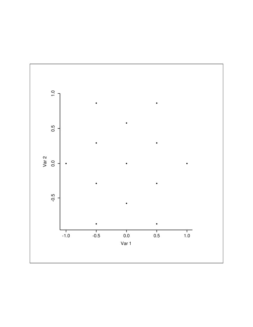
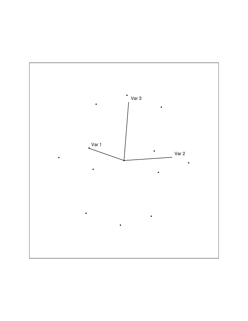
We replace a coarse particle with a configuration of 13 particles as shown in Fig. 4.1. A fine particle is put exactly at the position of the coarse particle, while 6 particles are put on the vertices of a hexagon centred on the position of the coarse particle. The remaining 6 particles are put on the vertices of two equilateral triangles parallel to the plane of the hexagon but on either side. All particles are put at equal distances from their nearest neighbours333We will deal with the value of shortly.. Such a lattice is the simplest possible arrangement that has minimum interstitial volume [\astronciteKittel1962]. In fact, it is the primitive cell of a face-centred cubic (cubic closed-packed) structure (see Fig. 4.1, left panel). Specifically, Table 4.1 gives the co-ordinates of the 13 fine particles at unit distance away from each other, in the reference frame of the coarse particle they replace.
| x | y | z | |
|---|---|---|---|
| 1 | 0 | 0 | 0 |
| 2 | 1 | 0 | 0 |
| 3 | -1 | 0 | 0 |
| 4 | 0.5 | 0 | |
| 5 | 0.5 | 0 | |
| 6 | -0.5 | 0 | |
| 7 | -0.5 | - | 0 |
| 8 | 0 | ||
| 9 | -0.5 | - | |
| 10 | 0.5 | - | |
| 11 | 0 | - | |
| 12 | -0.5 | -+ | |
| 13 | 0.5 | -+ |
The value of is of great importance as well as the value of the smoothing length of the fine particles, . They should be fine-tuned to minimise the deviation between the configuration of 13 fine particles and their parent coarse particle. Apart from reproducing the density profile of the parent coarse particle, the 13 fine particles should be positioned in such a way that they experience the same accelerations as if their parent coarse particle was present. Finally, we should take care that any density fluctuations input to the fine region after particle splitting are kept to a minimum. We will now calculate the density profile of the configuration of 13 fine particles in isolation as well as estimate any density fluctuations in a particle distribution due to the application of particle splitting.
4.3.2 Density profile of the configuration of 13 fine particles

In order to calculate the mean density profile of such a configuration of particles, we consider a sphere of radius centred on the central fine particle. We define the distance from the position of any one of the 12 outside fine particles to any point on this sphere as a function of and the angle (see Fig. 4.2) as
| (4.4) |
The mean density on the surface of the sphere is then evaluated using
| (4.5) |
where the first equation gives the total mass swept up by a shell of radius and infinitesimal thickness . We have used , the surface area of the sphere that is limited by the circle defined by angle (produced when , the dashed line on Fig. 4.2, is rotated about through an angle of ). is the mass of one of the fine particles ( where is the mass of the coarse particle) and its smoothing length (, where is the smoothing length of the coarse particle). We have not taken into account the mass of the central fine particle yet. Since we are averaging over all angles we have multiplied by 12 in order to account for all the outside fine particles.
The integral of Eqn. 4.3.2 becomes
| (4.6) |
where we have substituted . We have used the minus sign of the term to exchange the limits of the integral.
| (4.7) |
with the sum being the polynomial form of the M4-kernel (Eqn. 2.5).


The value of has not been defined yet. There are four different cases that we must take into account for the value of , depending on the value of . In particular:
-
1.
If the sphere centred on the central fine particle intercepts the two smoothing length sphere of an outside fine particle but not the one smoothing length sphere (, Fig. 4.2), then , where
(Fig. 4.2). Therefore, in this case,
and for Eqn. 4.7 we use the second part of the M4-kernel (Eqn. 2.5) for and .
- 2.
-
3.
If the sphere centred on the central fine particle intercepts both spheres (, Fig. 4.2), then the integral of Eqn. 4.7 breaks into two parts
(4.8) - 4.
The analytical calculation of these two integrals has now become trivial as, in every case we have to deal with integration of polynomial functions. In all other cases, the integral becomes equal to 0 due to the M4-kernel having compact support.
There are two parameters of the problem which we have not dealt with yet. Namely, the density of the central fine particle and the value of , the distance from the central to the outside fine particles. The calculation of the former is based on Eqn. 2.7 with the position of the central fine particle, the mass and the smoothing length of the fine particles. The total density for the ensemble of 13 fine particles is derived when we add the density of the central particle to the result of Eqns. 4.7 and/or 3. This is illustrated with the dashed curve on the left panel of Fig. 4.3, with the outside particles at a distance of .
is a free parameter in this problem and its value can be determined by minimising the integral
| (4.9) |


where is the density of the coarse particle444Its calculation is similar to that of the central fine particle. and is the density of the configuration of 13 fine particles that replace it. This integral gives the volume average of the absolute difference in the density estimates given by and as defined above. It is calculated numerically using the extended trapezoidal rule
where are the values of the function evaluated at () and () the constant step [\astroncitePress et al.1990].
The minimum of integral 4.9 gives (i.e. of ). The right panel of Fig. 4.3 shows and (solid and dashed curves respectively) when . The left panel of Fig. 4.5 shows a zoom on this, for between 0 and 0.2.
Examination of Fig. 4.3 shows that the shape of the density profile for the ensemble of fine particles is significantly different compared to the density profile of a coarse particle. The dip that appears in the former is due to the geometry of the fine particle configuration, i.e. the density drops with distance as we move away from the central particle before it rises again due to the outside particles.


We have also checked the behaviour of the density gradient. Fig. 4.4 shows the density gradient of a coarse particle (solid curve) and of the group of fine particles that replace it (dashed curve), calculated numerically555, where is the value of the density evaluated at () and () the constant step. for and (on the left and right panel respectively). One non-physical property of the M4-kernel is that the density gradient vanishes as , and therefore if two particles are very close the repulsive hydrostatic force between them is very small. This means that there will be a length scale below which artificial clustering of particles may occur. We would expect the density gradient of the 13 fine particles that will replace a coarse particle to behave at least similarly to that of their parent coarse particle. However, the density gradient of the group of fine particles has two minima (dashed lines of Fig. 4.4) which is worrying. Firstly, this means that there are going to be two length scales between which particles will be pulled towards the centre. Secondly, the smaller of these two length scales is a point of stable equilibrium, i.e. artificially clustered groups of particles may form and persist. Fortunately, it seems that there is an intrinsic geometrical constraint in the process of replacing coarse particles by fine ones. The fine particles are always positioned outside the outer of the two length scales where the hydrodynamical forces are reversed in direction. This means that our fine particles will always be positioned at a region where they will experience outward hydrodynamical forces. Problems may appear only if they are perturbed inwards and end up in the non-physical region. It appears that this does not happen in practice.


In order to explore if a group of fine particles can produce a density gradient that behaves similarly to that of a coarse particle, we have conducted another short parameter search for the best value of . For (right panel of Fig. 4.5 for ) the density gradient appears to take a shape similar to that of a coarse particle. However, we found that for , integral (4.9) gives a value for the absolute difference in the density estimates twice as large as the does.
4.3.3 Density stability with particle splitting


In this section we demonstrate that particle splitting does not significantly affect an existing density distribution of coarse particles. We have produced a uniform distribution of 500 particles in a box using periodic boundary conditions. We have evaluated the density both on the particle positions and on a square grid. Using the method described in §4.3.1, we then replaced each particle with 13 fine ones randomly oriented and we tried to reproduce the same uniform density allowing for a short settling of the fine particles. We have discovered that the value of , the distance of the 12 outside fine particle from the central fine particle, can influence our results significantly.
In particular, the amount of settling required after particle splitting for the density distribution to be identical to the initial settled box depended on this distance . We have used the ratio of the variance over the mean of the density distribution, , as the quantity that determines if our distribution is settled or not. We have settled until . The left panel of Fig. 4.6 shows the dependence of on immediately after the splitting. The right panel illustrates the density distribution of the initial settled box (before splitting). The minimum value of is for between and , with having the absolute minimum in both variance and mean of the density. Fig. 4.7 shows the density distribution of the box after splitting for (left panel) and (right panel). Thus, for the least settling is required. This applies for both the evaluation of density on particle positions and on the square grid.
Therefore, we finally decided that should neither be equal to nor (cf. §4.3.2) but . This is because it is the distribution of an ensemble of particles that we are particularly interested in, and not the density profile of a single particle. Any over-evaluation of the density around the position of the coarse particle (cf. Fig. 4.8 left panel) is expected to be treated appropriately by the hydrodynamical forces (dispersal of the ensemble of fine particles that replace it). The shape of the density gradient reassures us that this will happen (right panel of Fig. 4.8).
In §4.4.3 we will discuss the effects of particle splitting on a more realistic particle distribution.


4.3.4 Smoothing lengths for the fine particles
As shown in Fig. 4.6 & 4.7, there is an increase in the mean density of a uniform distribution of 500 particles after particle splitting is applied, even for the case of when this increase is minimum (i.e. minimum settling is required for the fine distribution to obtain again unit mean density). In particular, for this case the mean density is increased by 5.04%. Furthermore, the calculation of the number of neighbours for each fine particle does not always give the right result ().
In order to explore this further we have conducted another similar test. We have simulated a stable isothermal sphere in isolation and have applied particle splitting (in particular the nested splitting version) to its central region (the initial conditions are given in §4.4.2 and shown in Fig. 4.14). We have found that it is not only the number of neighbours that gives wrong results, but also the density inside and outside the fine sub-region is incorrectly modelled after splitting is applied. The reason for this is that there now exist particles of different mass in close contact. In particular, the method for finding the smoothing length for all particles is based on counting the number of their neighbours (§2.6). This makes fine particles just inside the sub-region boundary, which have coarse particles as neighbours, look for some of their neighbours in a region of lower resolution. Therefore, their smoothing length is over-estimated and their density under-estimated. The coarse particles just outside the sub-region boundary have fine particles as neighbours and look for their neighbours in a region of higher resolution. Thus, their smoothing length is under-estimated and their density over-estimated (top panel of Fig. 4.9 cf. with top panel of Fig. 4.14). However, there is an even more severe boundary effect disturbing the evolution of the fine simulation. Since the sub-region boundary is fixed in space, the fine particles should always be inside the boundary. Nevertheless, with the implementation of nested splitting fine particles penetrate through the non-moving coarse particles and end up at the other side of the boundary (bottom panel of Fig. 4.9 cf. with bottom panel of Fig. 4.14). The gravitational field around the boundary fine particles is not balanced as they are in contact with more massive particles from one side. This make them move to the other side of the boundary. In particular, they move through the gaps between the boundary coarse particles, occupying the potential energy gaps between those particles. This creates an expanding shell of fine particles similar to an artificial rarefraction wave which will eventually corrupt the evolution of the isothermal sphere even if the sphere may finally evolve to another stable equilibrium state.
Therefore, the new method clearly needs a special feature to eliminate these boundary effects. A possible solution would be to define a region on either side of the boundary, where both fine and coarse particles would have their smoothing length evolution constrained in order to create a smooth transition from the low to the high resolution and vice versa. However, this idea would be rather complicated to implement as the position and velocity of particles with respect to the boundary would need to be calculated at every time-step.
We have found a simpler method. It involves calculating the smoothing length of a particle by specifying the total mass of neighbours, rather than the number of neighbours. Specifically, the smoothing length of each particle is such that it contains 50 times its mass. We think this is more appropriate in our case where there exists mixing of particles with different mass. Away from the boundary, finding is exactly the same as before: there are equal mass neighbours. Close to the boundary, though, a coarse particle appears as 13 fine ones when is calculated for a fine particle, while it takes 13 fine particles to add one effective neighbour to a coarse particle. This method is valid as the volume of a coarse particle () is not significantly altered when the coarse particle is split with (§4.3.2)666For the first trial value of , the configuration of 13 fine particles has a radius of .. Close to the boundary, coarse particles have more than 50 neighbours and fine particles have less than 50, but both their smoothing lengths and densities are correctly modelled. In its numerical details, the method is implemented exactly the same way as before (§2.6), but the variable that we now use as a criterion for the acceptance of a trial smoothing length is the enclosed mass and not the number of enclosed neighbours. The notion of a particle always tracing constant mass is maintained and SPH with different mass particles preserves its Lagrangian character. The test simulation for the evolution of a stable isothermal sphere is repeated (§4.4.2) and shows that the new method for calculating greatly improves the treatment of the boundary as well as preventing the growth of numerical perturbations that may disturb the evolution of the stable isothermal sphere.


4.3.5 Velocities for the fine particles
To evaluate the velocity of each fine particle we use Eqn. 2.6
| (4.10) |
where , and are the velocity, position and smoothing length, respectively, of coarse particle , and is the position of fine particle . We do not sum contributions from coarse particles which are more than away from fine particle (i.e. ). Since each fine particle is contained within the radius of its parent coarse particle, the sum of Eqn. 4.10 is over the 50 neighbours of its parent particle. Obviously, the largest contribution comes from this parent particle, but Eqn. 4.10 guarantees that the velocity field around each coarse particle is accurately passed to the fine particles that replace it.
In all the tests to which particle splitting has been applied (§4.4), the velocity field is accurately represented by the fine particles after splitting occurs. The new method also conserves global linear and angular momenta.
4.3.6 Updating other fluid properties & numerical parameters
In “nested splitting”, the exact steps we follow in implementing particle splitting are:
-
•
We decide on the dimensions of the fine region. We count all the coarse particles that are inside this region at time when the method is initiated.
-
•
The fine particles that are produced are put in position by randomly rotating the co-ordinates given in Table 4.1 around the y- and z-axes.
- •
-
•
The fine particles are given the same temperature as their parent coarse particle. Taking into account that splitting is necessary in order for a simulation to be properly resolved up to the density where adiabatic heating initiates (chapter 2), this assumption of isothermality is valid for the fine particles, as all other particles remain isothermal as well. If particle splitting were necessary at later stages in regions with temperature gradients, temperatures could be calculated by interpolation in the same way as velocities.
-
•
All fine particles are put in the minimum time bin to make sure that the method sustains its accuracy. They are given the minimum time-step. If the multiple time-step method decides that they can be moved to a higher time bin, then this will happen as soon as it is allowed (§2.9). The extra computational cost of keeping some fine particles in the minimum time bin – even though this may not really be needed – is minimal. Nonetheless, our decision for the initial choice of time-step for the fine particles is dictated by the need to obtain the highest possible accuracy. Moving all the fine particles and updating their properties during the first time-steps after their introduction to the simulation also gives the code a cushion for correcting any values that do not match the local fluid properties around the fine particles.
-
•
The fine particles are given a splitting identifier indicating the level of splitting they represent, as the method may be applied several times in a simulation creating a series of nested simulations each at a higher resolution.
-
•
The total number of particles is updated to contain the fine particles. For book keeping purposes only, the central fine particle replaces its parent coarse particle in all variable arrays, while all other fine particles are put at the end of the arrays.
-
•
Finally, after the density of all fine particles is calculated, we can calculate the acceleration for these particles. For these calculations we use the usual SPH routines (§2.7). The fine particles are now ready to take part in the next cycle of the integration scheme and then the fine simulation starts.
-
•
At the end of all subsequent time-steps, the code checks for any coarse particles that may have crossed the sub-region boundary during the previous time-step. Then these coarse particles are split on-the-fly, without stopping the fine simulation. The code just repeats all the above steps for the coarse particles that have just entered the fine region. Fig. 4.10 shows the flow-chart of the algorithm that dictates the evolution of the fluid in time, after the on-the-fly splitting subroutines have been added.
In “on-the-fly splitting” we don’t have to stop the coarse simulation to apply particle splitting, but instead we use an automated test in the particle splitting subroutine. We calculate initially the density threshold, , above which the simulation stops resolving the Jeans mass. is given by Eqn. 4.3. Then we start the coarse simulation and particle splitting automatically initiates on-the-fly when particles exceed this density.
This way, we don’t have to apply splitting to particles unnecessarily, just because they are in spatial proximity to developing proto-condensations. Therefore, we can achieve even greater economy in computational cost, that can make the new method even more attractive and efficient. This is our preferred version of particle splitting and this is the method we apply to clump-clump collisions in the next chapter. In the following section we describe the application of both versions of particle splitting to standard test simulations.
4.4 Tests
We apply both versions of particle splitting to the central region of a collapse simulation, to see if there is propagation of boundary effects. We do the same for the central region of a simulation of a stable isothermal sphere, to show that the boundary effects mentioned in §4.3.4 have been eliminated by the new calculation of smoothing lengths. Finally, we apply both versions of particle splitting to the collapse simulation of a rotating, uniform-density, isothermal cloud with an m=2 perturbation (cf. chapter 3). We demonstrate that SPH with particle splitting gives very good results to this problem. We show that the Jeans condition for fragmentation provides a very strong test for the significance of numerical results. We also show the efficiency of the new method in terms of computational economy and in particular the superiority of “on-the-fly splitting”.
In quantifying the results of our tests, we need to be able to associate these results only with the performance of our numerical code. In order to decrease the numerical noise input by the initial distribution of particles, we perform all tests using clouds whose particles are taken initially to be on a lattice. In the sequel, we will refer to the particles of such simulations as “particles initially taken on a lattice”. To verify that the results of tests with particles initially taken on a lattice are not biased due to some preferred orientation of the initial lattice, we will also perform one simulation for each test where particles are taken initially from a “settled” distribution. Such a distribution of particles is produced when the particles are taken in random positions and then they are relaxed to uniform density, using the SPH formulation described in Whitworth et al. [\astronciteWhitworth et al.1995].
4.4.1 Collapse Simulation
We test both versions of particle splitting at the centre of a collapse simulation. This way we test the method under conditions of homogeneous inflow. Both implementations show good results. There is very little dispersion of fine particles out of the fine region and there is a well-defined boundary between the fine and the coarse regions.
The initial conditions consist of a spherical cloud of mass M = 1 M⊙ and radius R = 0.016 pc. The cloud has uniform density = 3.74 x 10⁻¹⁸ g cm-3 and uniform temperature T = 7.9 K. The ratio of thermal to gravitational energy is = 0.26 and the cloud has a Jeans mass of 0.2 M⊙, so that it is unstable and it collapses. There is no rotation. We have used 10,185 particles to simulate the cloud, initially taken on a lattice. For this test we use our complete self-gravitating SPH code (chapter 2). We also include adiabatic heating to slow down collapse. Adiabatic heating initiates at = 10-13 g cm-3. It is included in order to prevent small time-steps from occurring. Adiabatic heating is necessary at the very centre of the simulation, where matter accretes to form a central object. Outside the centre, isothermal collapse occurs. In this region, the collapsing gas evolves with a self-similar form, , as predicted by Bodenheimer & Sweigart [\astronciteBodenheimer & Sweigart1968].
Nevertheless, the time-step does get very small after some time. To prevent this, we have repeated the simulations using a sink particle to simulate the core of the accreted central object. With this, we allow accretion of more matter to the central object and we finally end up at a state where most coarse particles have entered the fine region and have been split.
A sink particle is a particle that accretes all matter that enters its radius. In this case the sink particles have a radius of 2 x 10⁻⁴ pc. There is only one sink particle at the centre of each simulation. The particles that lie inside this radius stop being active (i.e. their properties are not followed any further). The accreted particles have their mass decreased to zero and their mass is added to the mass of the sink. Therefore, the region just outside the sink is not very well evolved, as the active particles just outside the sink radius do not “see” the accreted particles inside the sink radius. As a result, these active particles look for neighbours only outside the sink. Their smoothing length is over-estimated and their densities under-estimated.
We stop all simulations when the time-step becomes less than 2 x 10⁻⁶ tff, so that it is computationally inefficient to continue (i.e. in order for time to progress by 10-2 tff we would need 5 times the run-time up to that point).
We present five different simulations: collapse using nested splitting without a sink, collapse using nested splitting with a sink, collapse using on-the-fly splitting without a sink, collapse using on-the-fly splitting with a sink, and collapse using nested splitting with particles initially taken from a settled distribution.


4.4.1.1. Isothermal collapse using nested splitting without a sink
The top panel of Fig. 4.11 shows the radial density profile of the sphere when nested splitting was applied with the fine region having a radius of 2 x 10⁻³ pc. The green points show fine particles and the black points coarse particles. The red line indicates the profile. The top panel of Fig. 4.11 shows the end of the simulation at time = 1.01 . For about 2 orders of magnitude in radius, we find that density complies well to the predicted profile, . Inside 3 x 10⁻⁵ pc the density increases rapidly due to the formation of a central core. The cloud has contracted to a radius of 6.3 x 10⁻³ pc. The maximum density at the centre of the cloud is = 4.8 x 10⁻¹¹ g cm-3. There are 69,861 particles in total, with 4,973 coarse particles having been split. Note that there are two boundary effects. Some fine particles have their density over-estimated immediately after their parent coarse particle is split (i.e. their first smoothing radius is smaller than it should be). Some other particles are attracted by the heavier coarse particles and temporarily exit the fine region. Both these effects are transient, as particle identification has proven that, although the effects are static with time, they are produced by different (new) fine particles at each time-step. This test shows that the boundary effects due to nested splitting are not significant as they do not alter the predicted density profile. SPH with the new method for calculating (§4.3.4) eventually remove any fluctuations input by the application of nested splitting.
4.4.1.2. Isothermal collapse using nested splitting with a sink
The bottom panel of Fig. 4.11 shows the radial density profile of the sphere when nested splitting was applied with the same radius for the fine region, but now with a sink particle having radius 2.0 x 10⁻⁴ pc, simulating the central accreted object. It is the end of the simulation at time = 1.05 . The radius of the sphere is 5.4 x 10⁻³ pc. Accretion to the centre of the cloud is not modelled properly due to the sink. The time-step does not decrease so rapidly and at the end of the simulation more matter has entered the fine region. In particular, there are 99,837 particles in total, with 7,471 coarse particles having been split. The radial density profile obeys the profile for one order of magnitude. A small density under-estimation is evident outside the sink radius due to the effects described at the end of §4.4.1. This test extends the conclusion that the boundary effects due to nested splitting are not significant in a case where most coarse particles () are split.
4.4.1.3. Isothermal collapse using on-the-fly splitting without a sink
The top panel of Fig. 4.12 shows the radial density profile of the sphere when on-the-fly splitting was applied. The density threshold is taken to be = 8.55 x 10⁻¹⁶ g cm-3. The green points show fine particles and the black points coarse particles. The red line indicates the profile. The top panel of Fig. 4.12 shows the end of the simulation at time = 1.01 . For about 2 orders of magnitude in radius, we find that density complies well to the predicted profile, . Inside 3 x 10⁻⁵ pc the density increases rapidly due to the formation of the central core. The density profile compares very well with the density profile of the nested splitting simulation (top panel of Fig. 4.11). The fine region has smaller radius than in the nested splitting simulation, but splitting happens again within the isothermal region (i.e. along the line), so that comparison between the two methods is legitimate. Again, the cloud has contracted to a radius of 6.3 x 10⁻³ pc, and the maximum density at the centre of the cloud is = 4.8 x 10⁻¹¹ g cm-3. In the on-the-fly splitting simulation there are only 46,917 particles in total, with 3,061 coarse particles having been split. Therefore, on-the-fly splitting, involving 20,000 particles less than nested splitting, advanced to the same state as nested splitting a lot faster, requiring less computational effort (the required memory and the size of the output files are proportional to the number of particles). Note that the two boundary effects are still present. Some fine particles have their density over-estimated immediately after their parent coarse particle is split (i.e. their first smoothing radius is smaller than it should be). Some other particles are attracted by the heavier coarse particles and temporarily exit the fine region moving to a region of lower resolution. Both these effects are again transient, as particle identification has proven that, although the effects are static with time, they are produced by different (new) fine particles at each time-step. This test shows that the boundary effects due to on-the-fly splitting are not significant as they do not alter the predicted density profile. SPH with the new method for calculating (§4.3.4) eventually removes any fluctuations input by the application of on-the-fly splitting. Comparison with nested splitting demonstrates that on-the-fly splitting produces the same results as nested splitting, much more efficiently.
4.4.1.4. Isothermal collapse using on-the-fly splitting with a sink
The bottom panel of Fig. 4.12 shows the radial density profile of the sphere when on-the-fly splitting was applied with the same density threshold, but now with a sink particle having radius 2.0 x 10⁻⁴ pc, simulating the central accreted object. It is the end of the simulation at time = 1.05 . The radius of the sphere is 5.4 x 10⁻³ pc. Accretion to the centre of the cloud is not modelled properly due to the sink. The time-step does not decrease so rapidly and at the end of the simulation more matter has entered the fine region. In particular, there are 86,817 particles in total, with 6,386 coarse particles having been split. The radial density profile obeys the profile for one order of magnitude. A small density under-estimation is evident outside the sink radius due to the effects described at the end of §4.4.1. The density profile of this test compares very well with that of the corresponding test of nesting splitting (i.e. nested splitting with a sink particle). This test extends the conclusion that the boundary effects due to on-the-fly splitting are not significant in a case where most coarse particles () are split.


4.4.1.5. Isothermal collapse using nested splitting with particles initially taken from a settled distribution
We have repeated the collapse simulation applying nested splitting to the centre of a cloud of 10,482 particles initially taken from a settled distribution with a uniform density of = 3.74 x 10⁻¹⁸ g cm-3. We have used the same initial conditions. We have simulated collapse with the same code as above (§4.4.1.1). The fine region has the same radius of 2 x 10⁻³ pc. There is no sink particle. Fig. 4.13 shows the radial density profile of the cloud at = 1.01 . The density complies well to the predicted profile, . It compares very well with the simulation of §4.4.1.1, when particles were initially taken on a lattice (top panel of Fig. 4.11). Note that in Fig. 4.13 there is more noise that in the top panel of Fig. 4.11. The cloud has contracted to a radius of 6.5 x 10⁻³ pc. The maximum density at the centre of the cloud is = 1.8 x 10⁻¹⁰ g cm-3. There are 74,394 particles in total, with 5,326 coarse particles having been split. This test rules out the possibility that the results presented above are biased due to some preferred orientation of the initial lattice.
4.4.2 Stable Isothermal Sphere
We test particle splitting on a simulation of a stable isothermal sphere. Both methods show again good results. The new calculation of (§4.3.4) has clearly eliminated previous inefficiencies in treating the fine region boundary. Fine particles still move towards the gaps between coarse particles at the boundary, but there is little penetration through the boundary. In particular, as the fine region slowly expands, coarse particles trapped in the expanding fine region are automatically split. Any fluctuations input by the application of particle splitting are being removed and the sphere settles towards the predicted density profile after a few free-fall times.
The initial conditions consist of a spherical cloud of mass M = 1 M⊙ and radius R = 0.1 pc. The cloud has central density = 3.04 x 10⁻²⁰ g cm-3 and uniform temperature T = 7.9 K. The density at the outer edge of the cloud is = 1.05 x 10⁻²⁰ g cm-3. The cloud is stable as it has = 3 (§2.11.3). There is no rotation. We have used 10,185 particles to simulate the cloud, initially taken on a lattice. Their positions are calculated according to the scheme given in §2.11.3. For this test we use our complete self-gravitating SPH code (chapter 2). The top panel of Fig. 4.14 shows the initial radial density profile of the cloud. We use crosses as the particles initially are on a lattice and the radial profile therefore consists of very few different points. The red line indicates the solution of Eqn. 2.54. The bottom panel of Fig. 4.14 is a thin equatorial slice ( pc) of the isothermal sphere showing the boundary between the coarse (black points) and the fine (green points) particles, immediately after nested splitting was applied within a radius of 3 x 10⁻² pc.
We present three different simulations for the evolution of a stable isothermal sphere: using nested splitting, using on-the-fly splitting and using nested splitting with particles initially taken from a settled distribution.
4.4.2.1. Stable isothermal sphere using nested splitting
The top panel of Fig. 4.15 shows the radial density profile of the isothermal sphere after = 8.17 , when nested splitting was applied with the fine region having a radius of 3 x 10⁻² pc. The green points show fine particles and the black points coarse particles. The red line indicates the solution of Eqn. 2.54. The density profile compares well with the initial one (top panel of Fig. 4.14). There are 22,833 particles in total with 1,054 coarse particles having been split. There are still some particles on either side of the boundary between the coarse and the fine regions having their density incorrectly modelled. These are basically new fine particles (split a few time-steps before) that have taken inappropriate initial values for their smoothing length. Their smoothing length and density will very soon settle to the expected values. However, the number of these particles is significantly reduced due to the application of the new method for calculating . Moreover, the deviation from the expected density profile for these particles is greatly reduced (cf. with the top panel of Fig. 4.9). The introduction of new fine particles into the simulation creates the opposite effect to neighbouring coarse particles: their smoothing length is over-estimated for a few time-steps and thus their density is under-estimated.


The fine particles inside the fine region boundary are still attracted by the coarse particles just outside the fine region. The fine region appears to expand slowly. However, there is now a clear boundary between the coarse and fine regions (bottom panel of Fig. 4.15 cf. with the bottom panel of Fig. 4.9). Fine particles do penetrate through the coarse particles. However, the majority of the latter are always kept outside the fine region. In fact, as fine particles slowly move to a region of lower density some coarse particles move inside the fine region radius and are automatically split. The coarse particles surrounded by fine particles in the bottom panel of Fig. 4.15 are split in the subsequent time-steps. This way, the number of coarse particles being split increases from 459 initially to 1,054 at the end of the simulation. The voids in the fine region shown in the equatorial slice of the bottom panel of Fig. 4.15 are projection effects produced when coarse particles exit the thin equatorial slice. Note that the thickness of the equatorial slice is less than, or of the order of the smoothing length of the coarse particles ( pc). Coarse particles exit temporarily the equatorial slice due to numerical noise in their inward motion (this motion is caused by the slowly expanding fine region). There is no way one can damp this noise at a scale smaller than the smoothing length of the particles.
We conclude that SPH with nested splitting constrains the cloud to remain at the same overall equilibrium state at all times, while the fine region boundary is permitted to evolve slowly within this global profile. In fact, the particles whose density deviates form the expected profile quickly have their density settled to the predicted values. This test shows that the boundary effects introduced by the application of nested splitting are not significant as the stable isothermal sphere retains its overall properties. It also demonstrates the efficiency of the new method for calculating (§4.3.4).

4.4.2.2. Stable isothermal sphere using on-the-fly splitting
The top panel of Fig. 4.16 shows the radial density profile of the isothermal sphere after = 8.59 , when on-the-fly splitting was applied with density threshold = 2.48 x 10⁻²⁰ g cm-3. The green points show fine particles and the black points coarse particles. The red line indicates the solution of Eqn. 2.54. The density profile compares very well with the initial one (top panel of Fig. 4.14). There are 27,057 particles in total with 1,406 coarse particles having been split. The density profile is similar to that of the nested splitting simulation (top panel of Fig. 4.15). Similar boundary effects can be observed in this test. There are some particles on either side of the boundary between the coarse and the fine regions having their density incorrectly modelled. These are basically new fine particles (split a few time-steps before) that have taken inappropriate initial values for their smoothing length. Their smoothing length and density will very soon settle to the expected values. The introduction of new fine particles into the simulation creates the opposite effect on neighbouring coarse particles: their smoothing length is over-estimated for a few time-steps and thus their density is under-estimated.
The fine particles inside the fine region are attracted by the coarse particles just outside the fine region. The fine region appears to expand slowly. However, there is again a clear boundary between the coarse and fine regions (bottom panel of Fig. 4.16 cf. with the bottom panel of Fig. 4.9; note that in on-the-fly splitting the fine region’s radius is larger). Fine particles do penetrate through the coarse particles. However, the majority of the latter are always kept outside the fine region. In fact, as fine particles slowly move to a region of lower density some coarse particles have their density estimates increased above the density threshold and are automatically split. The coarse particles surrounded by fine particles in the bottom panel of Fig. 4.16 are split in the subsequent time-steps. This way, the number of coarse particles being split increases from 959 initially to 1,406 at the end of the simulation. Therefore, a smaller fraction of coarse particles is split compared to the nested splitting simulation. The voids in the fine region shown in the equatorial slice of the bottom panel of Fig. 4.16 are again projection effects produced when coarse particles exit the thin equatorial slice. Note that the thickness of the equatorial slice is less than, or of the order of the smoothing length of the coarse particles ( pc). As in the previous simulation, coarse particles exit temporarily the equatorial slice due to numerical noise in their inward motion. There is no way one can damp this noise at a scale smaller than the smoothing length of the particles.
We conclude that SPH with on-the-fly splitting constrains the cloud to remain at the same overall equilibrium state at all times, while the fine region boundary is permitted to evolve slowly within this global profile. In fact, the particles whose density deviates form the expected profile quickly have their density settled to the predicted values. This test shows that the boundary effects introduced by the application of on-the-fly splitting are not significant as the stable isothermal sphere retains its overall properties. In this test, on-the-fly splitting produces similar results to nested splitting, again more efficiently.
4.4.2.3. Stable isothermal sphere using nested splitting with particles initially taken from a settled distribution
We have repeated the simulation for the evolution of the stable isothermal sphere applying nested splitting to the centre of a cloud of 10,482 particles initially taken from a settled distribution of uniform density. The particles are then positioned according to the scheme given in §2.11.3. We have used the same initial conditions and the same code as above (§4.4.2.1). The fine region has the same radius of 3 x 10⁻² pc. Fig. 4.17 shows the radial density profile of the cloud at = 6.63 . The density complies well to the initial profile (top panel of Fig. 4.14). It compares very well with the simulation of §4.4.2.1, when particles were initially taken on a lattice (top panel of Fig. 4.15). There are 22,602 particles in total, with 1,010 coarse particles having been split. The boundary effects are similar to those discussed above. In the simulation of §4.4.2.1, at = 6.63 , roughly the same number of coarse particles had been split. This test rules out the possibility that the results presented above are biased due to some preferred orientation of the initial lattice.
4.4.3 Rotating Cloud
Having tested the new method against a problem of homogeneous inflow as well as the evolution of a stable cloud, we now apply it to the standard test simulation, discussed in chapter 3. Application of the new method to a more realistic problem with known solution may reveal disadvantages of the new method that we have not calculated or thought of.
We apply the initial conditions used in the simulations of the previous chapter (§3.1), i.e. we use uniform-density, isothermal ( km s-1; T = 7.9 K; 0.26), rotating ( = 7.2 x 10⁻¹³ rad s-1; 0.16), spherical clouds of mass M = 1 M⊙ and radius R 0.02 pc, with particles cut initially from a face-centred cubic lattice and then given an m = 2 azimuthal perturbation by adjusting their spherical polar azimuthal coordinate, , to a value given by
We use our complete self-gravitating SPH code with 50 neighbours (chapter 2), including adiabatic heating. Our findings in the tests of the previous chapter, and in the tests of particle splitting in the present chapter, assist in fine-tuning the values of the initial number of particles and the density above which adiabatic heating switches on. This way, the simulations always obey the Jeans condition with minimum computational cost.
In chapter 3, we have shown that convergence to the results of Truelove et al. [\astronciteTruelove et al.1997, \astronciteTruelove et al.1998] and Klein et al. [\astronciteKlein et al.1999] can be achieved only with high resolution simulations. We have also shown that filamentary singularities can be obtained only if the simulations are evolved isothermally for sufficient time. The new method allows us to start a coarse simulation with low- to medium-resolution until it reaches the maximum resolvable density, (Eqn. 4.3), when particle splitting can be applied to increase the resolution 13-fold. If adiabatic heating starts before the fine simulation reaches its resolution limit, then the simulation obeys the Jeans condition at all times. Specifically, in the adiabatic heating regime the Jeans mass increases with increasing density (cf. Eqns. A.8 & 2.39) so that Eqn. 4.1 is always valid as long as adiabatic heating switches on before the fine simulation reaches its resolution limit. The higher the initial number of particles the longer the simulation can evolve isothermally, allowing for the use of a higher value for , the density above which adiabatic heating starts.
In order to use a high density for the switch to the adiabatic regime (=10-12 g cm-3), we have to start the simulation with no less than 40,000 particles. For comparison with the simulation of §3.3.1, we also present a simulation with =10-13 g cm-3. In order for such a simulation to obey the Jeans condition at all times, a cloud of as low as 10,000 particles initially can be used. In our effort to evolve both simulations with minimum computational cost, we use the minimum initial number of particles that allows the Jeans condition to be obeyed at all times for the above values of . In particular, the simulation with =10-12 g cm-3 starts with 40,000 particles and the simulation with =10-13 g cm-3 starts with 10,000 particles. We apply both versions of the new method to each simulation.
Bate & Burkert [\astronciteBate & Burkert1997] have shown that clouds of 10,000 particles do not resolve the binary formation. In contrast, clouds of 40,000 particles do resolve the formation of the binary and, in general, produce results very similar to those obtained with isothermal simulations of higher resolution.
The particle splitting simulation with 40,000 particles initially gives results consistent with those of Truelove et al. and Klein et al. as well as those presented in §3.3.4 for the 600,000 particle simulation, but with fewer particles, demonstrating the economy in computation achieved with particle splitting. The new method reduces the computational cost on two counts: we do not have to use high resolution from the beginning of the simulation and when we do increase the resolution, this does not have to happen everywhere but only in regions of interest.
Using particle splitting just before the 10,000 particle simulation violates the Jeans condition, proves to be sufficient to reproduce results of higher resolution simulations (Bate & Burkert [\astronciteBate & Burkert1997], §3.3.1, 3.4.2.2), but not the results of Truelove et al. [\astronciteTruelove et al.1997, \astronciteTruelove et al.1998], Klein et al. [\astronciteKlein et al.1999] and §3.3.4. This happens because the initial stages of the cloud evolution are not properly modelled due to low resolution. We present a simulation that cannot give results consistent with those of Truelove et al. and Klein et al. despite the fact that it obeys the Jeans condition at all times, to demonstrate that particle splitting is a necessary, but not a sufficient, condition for the reliability of a simulation.
Both versions of the new method produce similar results for each simulation. On-the-fly splitting is again more efficient than nested splitting in terms of computational cost. Tables 4.2 & 4.3 show a summary of our results. For comparison purposes, they also list the corresponding results of Truelove et al. [\astronciteTruelove et al.1998] and Klein et al. [\astronciteKlein et al.1999].
We do not need to present the simulation with particles initially taken from a settled distribution. The only case that the bar fragments is the nested splitting simulation for a cloud of 10,000 particles initially and the results of such a simulation with particles initially taken from a settled distribution are similar to those of §3.6. Therefore, we refer to the discussion of the results of §3.6.
All figures presented here are column density plots viewed along the rotation axis. The captions indicate the units of the colour tables. They also give the linear size of the figure and the time of the simulation.
4.4.3.1. Nested Splitting for a Cloud of 40,000 Particles
The top panel of Fig. 4.18 is a column density plot viewed along the rotation axis and shows the density projected on the x-y plane initially (at ), where the density enhancements indicate the m=2 perturbation. In a medium to high resolution simulation of a rotating, spherical, uniform, isothermal cloud with an m = 2 perturbation, the binary separation is expected to be 0.004 pc (§3.3). Taking into account the flattened shape that the cloud takes after 1 , the fine region in nested splitting takes a cylindrical shape and its radius is large enough to contain the binary formed and any other structure associated with it (e.g. spiral tails). The cylinder’s height is as large as the thickness of the disc formed (1/4 of the disc radius). Specifically, the fine region radius is 0.003 pc.


Nested splitting is applied after 1.244 , when the binary has started forming and the maximum density is about to exceed the density threshold, = 2.4 x 10⁻¹⁴ g cm-3, above which the simulation stops resolving the Jeans mass. Initially, 17,400 coarse particles lie inside the fine region radius and are split. The bottom panel of Fig. 4.18 is a column density plot immediately after the application of nested splitting. Note the smooth transition of the column density through the fine region boundary (its diameter is 0.006 pc while the linear size of the bottom panel of Fig. 4.18 is 0.008 pc).
In subsequent time-steps, all particles crossing the fine region radius are split on-the-fly. A well-defined binary forms and between the binary components a bar grows. The fine simulation would reach its resolution limit at = 4 x 10-12 g cm-3, but adiabatic heating starts at = 10-12 g cm-3 and the simulation obeys the Jeans condition at all times. The top panel of Fig. 4.19 shows the column density just before adiabatic heating initiates at 1.254 .
The top panel of Fig. 4.19 compares well with Fig. 12 of Truelove et al. [\astronciteTruelove et al.1998]; there are two elongated objects and a thin bar connecting them ( = 7.14 x 10⁻¹³ g cm-3).
The bottom panel of Fig. 4.19 shows the column density at the end of the simulation, 1.265 . There are 281,331 particles in total with 20,020 coarse particles having been split. The mass of each fragment is 0.02 M⊙ and its radius 7 AU. Their separation is 515 AU. The peak density of the simulation has risen to = 1.97 x 10⁻¹⁰ g cm-3. The bar has not fragmented. There is a well-defined contrast between the density of the binary components and the bar that connects them (2 orders of magnitude).
The final results compare well with those of Klein et al. [\astronciteKlein et al.1999] (their Fig. 2 - note that in Klein et al. adiabatic heating starts about one order of magnitude earlier).
The resolution of the simulation is sufficient that we can trust the result that the bar does not fragment up to 1.265 . In fact, the resolution of this simulation is equivalent to the resolution of a 520,000 particle simulation and the results are indeed similar to those of the simulation with the highest resolution we conducted without splitting in §3.3.4 (600,000). In particular, the peak density of the simulation is comparable to that of the simulation with 600,000 particles (see discussion in §3.3.4). This indicates the efficiency of nested splitting as only 281,331 particles have been used.
4.4.3.2. On-the-fly Splitting for a Cloud of 40,000 Particles
On-the-fly splitting is applied after 1.244 , when the maximum density is about to exceed the density threshold, = 2.4 x 10⁻¹⁴ g cm-3, over which the simulation stops resolving the Jeans mass. Initially, 2,955 coarse particles are split. The top panel of Fig. 4.20 is the first column density plot after the application of on-the-fly splitting (= 1.251 ). Note the smooth transition of the column density through the fine region boundary (within the red coloured area).
In subsequent time-steps, all particles whose density exceeds the density threshold are split on-the-fly. A well-defined binary forms and between the binary components a bar grows. The fine simulation would reach its resolution limit at = 4 x 10-12 g cm-3, but adiabatic heating starts at = 10-12 g cm-3 and the simulation obeys the Jeans condition at all times. The bottom panel of Fig. 4.20 shows the column density just before adiabatic heating starts at 1.258 .
The bottom panel of Fig. 4.20 compares well with Fig. 12 of Truelove et al. [\astronciteTruelove et al.1998]; there are two elongated objects and a thin bar connecting them ( = 6.86 x 10⁻¹³ g cm-3).
Fig. 4.21 shows the column density at the end of the simulation, 1.277 . There are 150,135 particles in total with 9,087 coarse particles having been split. The mass of each fragment is 0.03 M⊙ and its radius 10 AU. Their separation is 475 AU. The peak density of the simulation has risen to = 1.85 x 10⁻¹⁰ g cm-3. The bar has not fragmented. There is a well-defined contrast between the density of the binary components and the bar that connects them (2 orders of magnitude).
The final results compare well with those of Klein et al. [\astronciteKlein et al.1999] (their Fig. 2 - note that in Klein et al. adiabatic heating starts about one order of magnitude earlier).
The resolution of the simulation is sufficient that we can trust the result that the bar does not fragment up to 1.277 . In fact, the resolution of this simulation is equivalent to the resolution of a 520,000 particle simulation and the results are indeed similar to those of the simulation with the highest resolution we conducted without splitting in §3.3.4 (600,000). In particular, the peak density of the simulation is comparable to that of the simulation with 600,000 particles (see discussion in §3.3.4). This indicates the efficiency of on-the-fly splitting as only 150,135 particles have been used.
Comparison between the results of the on-the-fly splitting and the nested splitting simulations clearly indicates that the results are similar (see Tables 4.2 & 4.3), although the on-the-fly splitting simulation has progressed more in time (the binary components have accreted more matter, they are closer and the bar is more inclined). However, on-the-fly splitting is much more efficient in obtaining them (using 131,196 less particles in total).
4.4.3.3. Nested Splitting for a Cloud of 10,000 Particles
The top panel of Fig. 4.22 is a column density plot viewed along the rotation axis and shows the density projected on the x-y plane initially (at ) for a cloud of 10,000 particles, where the density enhancements indicate the m=2 perturbation. The coarser resolution used here does not change the initial appearance of the cloud (cf. the top panel of Fig. 4.18). Following the same reasoning as in §4.4.3.1, the fine region is cylindrical with the radius now taken to be 0.002 pc (the expected bar length is extracted from Fig. 7 of Bate & Burkert [\astronciteBate & Burkert1997]).


Nested splitting is applied after 1.105 , when the maximum density is about to exceed the density threshold, = 1.5 x 10⁻¹⁵ g cm-3, over which the simulation stops resolving the Jeans mass. At this time, the binary has not formed yet and the centre of the cloud has just started collapsing after the initial expansion phase [\astronciteBate & Burkert1997]. Initially, 705 coarse particles lie inside the fine region radius and are split. The bottom panel of Fig. 4.22 is a column density plot immediately after the application of nested splitting. Note that the lattice which the particles were initially taken on has not broken yet. Also note the smooth transition of the column density through the fine region boundary (its diameter is 0.004 pc while the size of the bottom panel of Fig. 4.22 is 0.008 pc). The density of the fine particles is emphasised due to effects similar to those discussed in §4.4.2.1 and the small dynamic range of the bottom panel of Fig. 4.22.
In subsequent time-steps, all particles crossing the fine region radius are split on-the-fly. A central density enhancement grows and later forms a bar. On either side of the bar spiral tails form due to rotation. At both ends of the bar two objects finally form at = 1.265 . The fine simulation would reach its resolution limit at = 2.53 x 10⁻¹³ g cm-3, but adiabatic heating starts at = 10-13 g cm-3 and the simulation obeys the Jeans condition at all times. The top panel of Fig. 4.23 shows the column density just before adiabatic heating starts at 1.265 . Subsequently, the bar fragments producing three fragments, one at the centre and two at equal distances from the centre.
This is in accordance with the findings of the low resolution run of Bate & Burkert [\astronciteBate & Burkert1997], where the binary formation is not resolved and just a bar forms that later fragments into multiple fragments. However, in this simulation, with application of nested splitting, the binary forms, although at a later stage than expected.
The bottom panel of Fig. 4.23 shows the column density at the end of the simulation, 1.301 . There are 55,125 particles in total with 3,794 coarse particles having been split. The mass of the binary fragments is 0.06 M⊙ and of the bar fragments 0.01 M⊙. The binary fragments have radii of 25 AU. The bar is 410 AU long. The peak density of the simulation has risen to = 2.14 x 10⁻¹¹ g cm-3. The bar fragments as it does in the corresponding runs of Bate & Burkert [\astronciteBate & Burkert1997] and those of §3.3.1, 3.4.2.2.
Clearly, the evolution of this simulation does not imitate the evolution predicted by the high resolution simulations of Truelove et al. [\astronciteTruelove et al.1997, \astronciteTruelove et al.1998], Klein et al. [\astronciteKlein et al.1999] and §3.3.4 (see Tables 4.2 & 4.3).


The equivalent resolution from the beginning of the simulation
At the centre of this simulation the resolution is equivalent to that of a simulation with 130,000 coarse particles. We have constructed such a test to compare with the above simulation. We have used the same initial conditions with 130,000 particles initially taken on a lattice. Adiabatic heating initiates at = 10-13 g cm-3. Particle splitting is not applied.
Fig. 4.24 shows the end of the 130,000 particles simulation, at 1.291 . In this case, the binary formation is resolved (forms at 1.239 ). The bar between the binary components does fragment, i.e. the results are similar to the simulations of Bate & Burkert [\astronciteBate & Burkert1997] and those of §3.3.1, 3.4.2.2.
The difference between the results of this run and the results of the above simulation with only 10,000 particles initially is due to the low resolution initial phase of the latter simulation. In particular, in the latter simulation the initial expansion and the subsequent collapse that leads to the formation of the binary [\astronciteBate & Burkert1997] are not properly modelled (due to poor sampling) and this causes the delayed formation of the binary. The application of nested splitting and the fact that the Jeans condition is obeyed clearly assists in the eventual formation of the binary (cf. the result of the 10,000 particle simulation of Bate & Burkert [\astronciteBate & Burkert1997]).
This conclusion is confirmed by the results of simulations of 20,000 and 30,000 particles initially, with application of on-the-fly splitting. In particular, we find that in these two runs the binary formation is resolved. Moreover, the evolution of the 30,000 particle simulation is closer to the converged solution of Bate & Burkert [\astronciteBate & Burkert1997]. However, application of particle splitting, despite assisting this simulation in creating the binary that would not be formed otherwise, can not guarantee solving all problems, due to poor sampling.
4.4.3.4. On-the-fly Splitting for a Cloud of 10,000 Particles
On-the-fly splitting is applied to the cloud of 10,000 particles after 1.105 , when the maximum density is about to exceed the density threshold, = 1.5 x 10⁻¹⁵ g cm-3, over which the simulation stops resolving the Jeans mass. Initially, 3,146 coarse particles are split. The top panel of Fig. 4.25 is the first column density plot after the application of on-the-fly splitting (=1.142 ). Note the smooth transition of the column density through the fine region boundary (within the green coloured area). Note that the lattice which the particles were initially taken on has not broken yet. Within the few time-steps elapsed after the first coarse particles were split, a rugged appearance similar to the bottom panel of Fig. 4.22 has been smoothed out as it did in §4.4.2.2. Due to the low density threshold, many coarse particles are split on the fly within these few time-steps. At =1.142 , the binary has not formed yet and the centre of the cloud has just started collapsing after the initial expansion phase [\astronciteBate & Burkert1997].
In subsequent time-steps, all particles whose density exceeds the density threshold are split on-the-fly. A central density enhancement grows and later forms a bar. On either side of the bar spiral tails form due to rotation. The fine simulation would reach its resolution limit at = 2.53 x 10⁻¹³ g cm-3, but adiabatic heating starts at = 10-13 g cm-3 and the simulation obeys the Jeans condition at all times.
The bottom panel of Fig. 4.25 shows the column density just before adiabatic heating starts at 1.293 . At both ends of the bar two objects finally form at = 1.317 . Subsequently, the bar does not fragment. This result is in accordance with the findings of the high resolution simulations of Truelove et al. [\astronciteTruelove et al.1997, \astronciteTruelove et al.1998], Klein et al. [\astronciteKlein et al.1999] and §3.3.4, where the bar does not fragment. However, in this simulation, due to the initial coarse resolution phase, the binary forms at a much later stage than expected. Fig. 4.26 shows the column density at the end of the simulation (1.326 ). The density contrast between the binary components and the bar that connects them is greater than one order of magnitude. There are 96,255 particles in total with 7,219 coarse particles having been split. The mass of each binary fragment is 0.06 M⊙ and its radius 40 AU. The bar is 270 AU long. The peak density of the simulation has risen to = 5.04 x 10⁻¹² g cm-3.
In this simulation the initial expansion and the subsequent collapse that leads to the formation of the binary [\astronciteBate & Burkert1997] are not properly modelled (due to poor sampling) and this causes the delayed formation of the binary. The application of on-the-fly splitting and the fact the Jeans condition is obeyed clearly assists in the eventual formation of the binary (cf. the result of the 10,000 particle simulation of Bate & Burkert [\astronciteBate & Burkert1997]). The fact that the binary forms later than in all other low resolution simulations of §3.4 as well as the above simulation (nested splitting with 10,000 particles initially) can be attributed to the large number of coarse particles being split almost simultaneously at the initial stages. During the collapse phase following the initial expansion, many coarse particles obtain density larger than the low density threshold we have used. We have used such a low value for (1.5 x 10⁻¹⁵ g cm-3) due to the small initial number of particles. The simultaneous splitting of few thousand particles introduced excess density perturbations to the simulation. SPH and the new method for calculating have been shown to be efficient in eliminating such perturbations. This is why we finally obtain the right result.
Comparison between the results of the on-the-fly splitting and the nested splitting simulations with 10,000 particles initially, shows that only with on-the-fly splitting we can reproduce the results of the high resolution simulations of Truelove et al. [\astronciteTruelove et al.1997, \astronciteTruelove et al.1998], Klein et al. [\astronciteKlein et al.1999] and §3.3.4 (see Tables 4.2 & 4.3). However, with the low density threshold set due to the small initial number of particles the computational cost of the on-the-fly splitting simulation grows considerably. Therefore, accuracy has been achieved at the expense of computational efficiency. This is against one of the primary aims of the new method that is designed to gain both in accuracy and computational efficiency. This confirms our previous conclusion that particle splitting, the way it has been formulated in this work, is a necessary, but not a sufficient, condition for the reliability and efficiency of a simulation.
4.4.4 Conclusions
| Simulation | Particles | / g cm-3 | / g cm-3 | / | / | / | / g cm-3 |
|---|---|---|---|---|---|---|---|
| Nested | 40,000 | 10-12 | 2.4 x 10⁻¹⁴ | 1.244 | 1.244 | 1.254 | 7.14 x 10⁻¹³ |
| On-the-fly | 40,000 | 10-12 | 2.4 x 10⁻¹⁴ | 1.251 | 1.244 | 1.258 | 6.86 x 10⁻¹³ |
| Nested | 10,000 | 10-13 | 1.5 x 10⁻¹⁵ | 1.105 | 1.265 | 1.265 | 8.52 x 10⁻¹⁴ |
| On-the-fly | 10,000 | 10-13 | 1.5 x 10⁻¹⁵ | 1.142 | 1.317 | 1.293 | 7.81 x 10⁻¹⁴ |
| Truelove (1998) | R32 | – | – | – | – | 1.317 | 3.91 x 10⁻¹³ |
| Klein (1998) | R32 | – | – | – | – | 1.304 | 8.97 x 10⁻¹⁵ |
| Simulation | Particles | / g cm-3 | / | Bar Fragm. | / | / g cm-3 | Particles |
|---|---|---|---|---|---|---|---|
| Nested | 40,000 | 10-12 | 1.265 | 0 | N/A | 1.97 x 10⁻¹⁰ | 281,331 |
| On-the-fly | 40,000 | 10-12 | 1.277 | 0 | N/A | 1.85 x 10⁻¹⁰ | 150,135 |
| Nested | 10,000 | 10-13 | 1.301 | 3 | 1.281 | 2.14 x 10⁻¹¹ | 55,125 |
| On-the-fly | 10,000 | 10-13 | 1.326 | 0 | N/A | 5.04 x 10⁻¹² | 96,255 |
| Truelove (1998) | R32 | – | 1.319 | 0 | N/A | 5 x 10⁻¹⁰ | R131,072 |
| Klein (1998) | R32 | – | 1.351 | 0 | N/A | 1.88 x 10⁻¹¹ | R4,096 |
The first two tests (§4.4.1 & 4.4.2) have proven that the new method for calculating (§4.3.4) has greatly reduced the boundary perturbations introduced by the application of particle splitting to the regions where fine and coarse particles are in contact. In particular, the collapse simulations (§4.4.1) show that there is no outward propagation of the fine region boundary in cases of inflow, which are the flows usually investigated in simulations of Star Formation. It also shows that the fine region reproduces the expected density profiles.
The simulation of the evolution of a stable isothermal sphere (§4.4.2) shows that there is a distinct boundary between the fine and the coarse regions. The boundary may expand in cases of quiescent evolution of stable spheres, but the overall density profile accurately obeys the predicted one, irrespectively of the size of the fine region. Both tests have revealed that the on the fly version of particle splitting is much more efficient in terms of computational cost. In principle, nested splitting could be superior to on-the-fly splitting if the boundary perturbations mentioned in §4.3.4 persisted after the implementation of the new method for calculating , as in nested splitting the fine region is larger than it really needs to be. This could prevent the boundary effects from propagating inwards and corrupting the simulation. However, both tests show that the boundary effects of both versions of the new method have been eliminated to a large extent and that the insignificant errors produced by particle splitting are similar in both versions of the method. Therefore, on-the-fly splitting can be safely used as it is superior in terms of computational cost.
We have also applied particle splitting to collapse simulations like those of the previous chapter. We conclude that the simulations with 40,000 particles initially, that use a sufficiently high density for the switch to adiabatic heating (=10-12 g cm-3) while obeying the Jeans condition at all times, reproduce the results of Truelove et al. [\astronciteTruelove et al.1998], of Klein et al. [\astronciteKlein et al.1999], and of our highest resolution simulation of §3.3.4 (600,000), but with only 200,000 particles in total at the final stages. The resolution of these simulations is equivalent to the resolution of a simulation with 520,000 particles, which clearly indicates the efficiency of particle splitting. In particular, with particle splitting we achieved economy in memory and economy in CPU. A summary of our results is given in Tables 4.2 & 4.3.
With particle splitting the simulation obeys the Jeans condition at all times with great computational gain. Our new method has succeeded in meeting the objectives we have set in §4.2. We can now apply it to simulations of clump-clump collisions.
On-the-fly splitting is more efficient than nested splitting, as even less particles are required. This is due to the fact that in on-the-fly splitting no particles are split unnecessarily. On-the-fly splitting is our preferred version of the new method. We will use on-the-fly splitting in simulations of clump-clump collisions in the next chapter.
In all simulations presented here, the Jeans condition is always obeyed and therefore there are no artificial fragments. This demonstrates the Jeans condition for fragmentation provides a very strong test for the significance of numerical results.
However, with the simulations with 10,000 initially and =10-13 g cm-3, we have shown that particle splitting in response to the imminent violation of the Jeans condition is a necessary, but not a sufficient, condition for the reliability and efficiency of a simulation. In particular, the low resolution of the initial stages of the cloud evolution has prevented the nested splitting simulation from reproducing the result of finite difference simulations of the same problem. It has also prevented the on-the-fly splitting simulation from obtaining this result efficiently.
Chapter 5 On-the-fly Splitting Simulations of Clump-Clump Collisions
Simulations of cloud-cloud collisions [\astronciteChapman et al.1992, \astroncitePongracic et al.1992, \astronciteTurner et al.1995, \astronciteWhitworth et al.1995, \astronciteBhattal et al.1998] evolve over several orders of magnitude in density and involve fragmentation to produce protostellar objects. Therefore, it is essential that fragmentation is properly modelled, i.e. the resolution is sufficient that the Jeans condition is always obeyed. The particle splitting simulations of the standard test with only 10,000 particles initially (§4.4.3) have shown that the Jeans condition is a necessary but not sufficient condition for reliable simulations; in that case the initial expansion and the subsequent collapse of the cloud were not properly modelled.
The cloud-cloud collision simulations of Bhattal et al. [\astronciteBhattal et al.1998] were conducted with small numbers of particles (2,000-8,000 per cloud) and implemented with a constant gravity softening, . However, small numbers of particles lead to violation of the Jeans condition and inaccurate modelling of the density field (§3.3.5, 3.4 & 4.1). Also Bate & Burkert [\astronciteBate & Burkert1997] have demonstrated that the implementation of constant -softening can be very misleading for SPH calculations with gravity, as it can both artificially induce fragmentation of Jeans stable lumps and/or stabilise Jeans unstable lumps against collapse, depending on the ratio (§4.1).
Therefore, it is worth conducting new high resolution simulations in which the Jeans condition is explicitly monitored and obeyed, in order to obtain a more detailed understanding of the processes involved. In this chapter, we perform such high resolution simulations of clump-clump collisions by applying particle splitting, and in particular the on-the-fly splitting version.
In chapter 4, we have shown that on-the-fly splitting is both a reliable and a computationally efficient method. Therefore, with on-the-fly splitting, we can overcome the problem of insufficient resolution for modelling fragmentation and so we can obtain credible results. We use -softening, i.e. we set . All particles have an individual time-varying .
We perform three simulations starting from the initial conditions used by Bhattal et al. [\astronciteBhattal et al.1998] in order to make direct comparisons with their results, and hence to quantify the effects of low resolution and -softening on those results (§5.2). We also investigate fragmentation induced by collisions between low-mass clumps by performing a series of simulations with various combinations of relative velocity and impact parameter (§5.3). We note that collisions of clumps from the low-mass end of the clump mass function have not been investigated before.
Previous collision simulations have shown that all fragmentation events happen in the shocked gas layer formed at the interface of the collision. It is therefore very important that the formation of this layer is properly modelled. In the following section, we define the appropriate minimum initial number of particles for our simulations to obey the Jeans condition at all times, and to resolve the formation of this shock. We also define the physical and numerical initial conditions for our simulations.
5.1 Initial conditions
| /km s-1 | /K | /km s-1 | /km s-1 | |||||
|---|---|---|---|---|---|---|---|---|
| 5 | 1 | 224 | 1,410 | 0.45 | 0.2 | 10 | 1.0 | 0.5 |
| 10 | 1,258 | 14,099 | 0.77 | 0.36 | 32 | 1.0 | 0.5 | |
| 75 | 5,699 | 105,739 | 1.31 | 0.59 | 87 | 1.0 | 0.5 | |
| 100 | 7,072 | 140,985 | 1.43 | 0.63 | 100 | 1.0 | 0.5 | |
| 9 | 1 | 300 | 1,410 | 0.33 | 0.2 | 10 | 1.8 | 0.9 |
| 10 | 1,688 | 14,099 | 0.57 | 0.36 | 32 | 1.8 | 0.9 | |
| 75 | 7,646 | 105,739 | 0.97 | 0.59 | 87 | 1.8 | 0.9 | |
| 100 | 9,487 | 140,985 | 1.07 | 0.63 | 100 | 1.8 | 0.9 | |
| 10 | 1 | 317 | 1,410 | 0.32 | 0.2 | 10 | 2.0 | 1.0 |
| 10 | 1,779 | 14,099 | 0.54 | 0.36 | 32 | 2.0 | 1.0 | |
| 75 | 8,060 | 105,739 | 0.92 | 0.59 | 87 | 2.0 | 1.0 | |
| 100 | 10,000 | 140,985 | 1.01 | 0.63 | 100 | 2.0 | 1.0 | |
| 15 | 1 | 388 | 1,410 | 0.26 | 0.2 | 10 | 1.0 | 0.5 |
| 10 | 2,178 | 14,099 | 0.44 | 0.36 | 32 | 1.0 | 0.5 | |
| 75 | 9,871 | 105,739 | 0.75 | 0.59 | 87 | 1.0 | 0.5 | |
| 100 | 12,248 | 140,985 | 0.83 | 0.63 | 100 | 1.0 | 0.5 |
When two clouds collide, a layer of shocked gas forms at the interface between the clouds [\astronciteChapman et al.1992, \astroncitePongracic et al.1992, \astronciteTurner et al.1995, \astronciteWhitworth et al.1995, \astronciteBhattal et al.1998]. The layer eventually fragments producing groups of protostars. Whitworth et al. [\astronciteWhitworth et al.1994b] have shown that the mass of a fragment, , produced in such a shocked layer is given by
| (5.1) |
where is the effective sound speed of the gas in the shocked layer, is the initial pre-shock density of each one of the two clouds involved in the collision and is the Mach number of the collision, defined as the ratio of the relative velocity of the clouds, , to (, where is the bulk velocity of each cloud).
The pre-shock density of each cloud, , is given by
| (5.2) |
if we make the assumption that the clouds are in hydrostatic balance (i.e. in an equilibrium state). is the cloud mass and is the effective pre-shock sound speed, i.e. a sound speed which represents thermal and turbulent pressure.
| (5.3) |
In order for the formation of these fragments to be resolved, their mass must be larger, or of the order of, the minimum mass resolvable by SPH, 2. Substituting = we obtain,
| (5.4) |
and hence
| (5.5) |
| (5.6) |
where we have used =0.2 km s-1 for the post-shock sound speed, or equivalently =10 K for the post-shock temperature. This is a reasonable assumption since for typical post-shock densities, the gas cools very rapidly and efficiently down to 10 K. The third column of Table 5.1 lists the minimum initial numbers of particles, , needed to resolve fragmentation in the shocked layer for the different values of and . In §2.11.1, we have shown that the shock is adequately modelled with our code for =0.5 km s-1 (=5).
Above g cm-3 the gas heats up adiabatically, as described in chapter 2. In chapter 3, we have used different values for in order to explore the performance of our code under different circumstances. The value of above which adiabatic heating switches on is defined by where heating due to gravitational collapse exceeds the rate of cooling by dust – because the dust becomes optically thick to its own radiation (e.g. Whitworth et al. [\astronciteWhitworth et al.1998]). is given by
where and are the Planck and Boltzmann constants respectively and is the speed of light. If we substitute the values of the constants, =10 K and assume that the gas is molecular, then we arrive to a value for g cm-3.
In order for the Jeans condition to be obeyed not just for the first fragments formed in the layer but also up to = 10-14 g cm-3, we need
| (5.7) |
(Eqn. 4.2). To find the minimum initial number of particles, , needed for the Jeans condition to be obeyed in the layer up to = 10-14 g cm-3, we divide by 13 the number of particles given by Eqn. 4.2, as we can increase the number of particles 13-fold by using particle splitting once. The fourth column of Table 5.1 lists the values of for the different values of .
From Table 5.1 we observe that is always larger than so that we always use as the initial number of particles in our simulations. In all cases, we use =50.
Collisions between low-mass clumps (=10 M⊙) seem to be the most computationally efficient to explore as they only need 15,000 particles initially for the Jeans condition to be obeyed at all times. Collisions between such clumps have not been investigated before. In all cases, two equal mass clumps of 10 M⊙ collide with opposite bulk velocity vectors. In molecular clouds with hierarchical substructure, collisions between clumps at the same level of the hierarchy (i.e. with comparable mass) are the most probable [\astronciteScalo1985].
We have conducted simulations with =5, 10, and 15 and with , the ratio of the impact parameter to the radius of the cloud, satisfying =0.0, 0.2, 0.4, 0.6 and 0.8. Whitworth et al. [\astronciteWhitworth et al.1994a] have argued that the equations used to estimate are approximately valid not only for head-on collisions (=0.0) but also for collisions with 0.7. The =0.8 collisions are conducted only for completeness, as the clumps do not interact strongly, even in the slowest collision (=5).
We also repeat three simulations using the initial conditions of Bhattal et al. [\astronciteBhattal et al.1998] with the Jeans condition obeyed at all times (seventh row in Table 5.1). Our aim is to make a direct comparison of our results with theirs, in order to be able to quantify the effect of fragmentation being properly modelled and the benefit of using particle splitting. We perform the simulations with =0.2, 0.4 and 0.5, as the first and the third ones are categorised by Bhattal et al. as having different mechanisms in play for the formation of binary/multiple protostellar systems (rotational instability in a disc vs. fragmentation of the layer). We also perform the second one as Bhattal et al. claim that it combines both mechanisms.
From Table 5.1 we see that for 10 M⊙ clumps, the pre-shock sound speed 0.35 km s-1 so that the pre-shock temperature of the clumps is 35 K. For typical post-shock densities cooling of the gas is very rapid and efficient so that it cools down to 10 K in the shocked layer very quickly. In order to be able to model this behaviour, we have slightly altered our barotropic equation of state (Eqn. 2.4) so that
| (5.8) |
where 0.35 km s-1, 0.2 km s-1 and =1.2 x 10⁻²⁰ g cm-3. is the density at which cooling initiates [\astronciteTohline1982]. This equation of state can be divided into four regimes. An isothermal regime with =35 K for densities below . A cooling stage, approximating to for densities just above , until the temperature reaches =10 K. The temperature then remains constant at =10 K for densities below . Finally, the gas heats up adiabatically above g cm-3.
We can summarise our initial conditions as follows. Two equal mass clumps collide with equal but opposite velocities. In repeating the simulations of Bhattal et al. we use =75 M⊙, 0.6 km s-1 (corresponding to =100 K); =9 (corresponding to =0.9 km s-1), =0.2, 0.4 and 0.5, and 110,000 particles per clump. In the second set of simulations, which we call low-mass clump collisions, we use =10 M⊙, 0.35 km s-1 (corresponding to =35 K); =5, 10, 15 (corresponding to =0.5, 1.0 and 1.5 km s-1), =0.0, 0.2, 0.4, 0.6 and 0.8, and 15,000 particles per clump.


In all cases, the clumps are stable isothermal spheres made with a procedure similar to that of §2.11.3. The particles, before they are moved to their final positions, are relaxed to uniform density, as they were initially taken from a random distribution (this relaxed distribution is what we called in previous chapters a “settled” distribution). The colliding clumps are taken to be touching before the simulations start, to save computational time. During the preceding approach of the colliding clouds, mutual tidal distortion will be small because . We use our full self-gravitating SPH code (chapter 2) with the above barotropic equation of state (Eqn. 5.8); we use -softening with our TCG method (§2.5); we use =50; and we use on-the-fly splitting at = = 6.0 x 10⁻¹⁷ g cm-3, as at this stage the Jeans condition would otherwise stop being obeyed. After application of particle splitting, adiabatic heating starts before the fine simulation reaches its resolution limit. Therefore, the Jeans condition is obeyed all the way up to the highest densities we can achieve.
We use false-colour column density plots to present our results. All structure formed is contained within a single layer and therefore such plots are not greatly confused by projection effects. Column density plots are preferred to particle plots as the former give a more accurate representation of the total density field, and of what would be seen in optically thin molecular-line (or dust-continuum) radiation, assuming a uniform excitation temperature (or dust temperature). We do not use contour plots, as we believe that colour column density plots are easier to read and give more information. The figure captions give the linear size of each plot and the plane onto which mass is projected. They also give the time of the snapshot they represent and the units of the colour table. We have taken the clouds always to collide along the x-axis, with offset parallel to the y-axis.
In all cases, when a fragment forms, its linear density profile appears like a normal distribution around the peak density. At the end of our simulations, this profile is very steep. To infer its mass, we take the fragment to extend out to 3-, where is the FWHM, and we measure the mass within this radius. This method gives good results for the mass and the radius of spherical as well as disc-like objects.
5.2 Repeating the Simulations of Bhattal et al.
5.2.1 Simulation with =75 M⊙ and =0.2
Bhattal et al. [\astronciteBhattal et al.1998] found that for low- collisions a single spherical protostellar object formed at the centre of the collision and then accreted material from the spindle-shaped filament. The protostellar object soon became disc-like and grew in mass and angular momentum as the offset between the opposing accretion flows along the spindle increased. Several accretion-induced rotational instability events took place as the primary protostellar disc ejected material and angular momentum through spiral arms. The ejected material interacted with the accretion flows and produced multiple lower mass companions to the massive primary. The primary had mass between 20-60 M⊙. The low-mass companions formed were not always resolved properly, as in some cases they contained less than 50 particles. Bhattal et al. used a constant -softening with 500 AU, so that they could not resolve the formation of an object until its size became 500 AU.
Our simulation evolves with very small time-step due to the large number of particles. After about 10,000 time-steps, it becomes extremely inefficient to continue the simulation, as even if the time-step did not decrease any further, after another 10,000 time-steps the time would only progress by about 1% of the total time that far. Therefore, we have terminated our simulation at that point, after 0.64 Myr. There are 260,000 particles at the end.
The fact that our simulation has to stop very early prevents us from presenting figures with the time evolution of properties such as the mass, angular momentum and radius of fragments or the binding energies of groups of protostars.
After 0.61 Myr, a network of filaments forms within the shocked layer. Protostellar objects start forming at the intercepts of the filaments. On-the-fly splitting is applied at 0.63 Myr. In total, four objects have formed via fragmentation of the filaments when the simulation terminates. Two of them quickly merge. At the end of the simulation (0.64 Myr), three disc-like objects are still accreting matter from the filaments. They are already centrally condensed. They are rotating fast and are attended by thin spiral arms. An offset develops between the opposing accretion flows and the inflowing material steadily increases the specific angular momentum of the discs. They are spinning increasingly fast. At this early stage of the evolution there is no sign of interaction between the spiral arms and the accretion flows. We believe that secondary companions to the discs may eventually form in our simulation via interaction between the spiral arms and the accretion flows. However, we note that the accretion flows in our simulation are extremely homogeneous, and not lumpy as they are in the simulation of Bhattal et al.
The three discs are still in the sub-solar mass range, in accordance with the mass evolution of Fig. 3 of Bhattal et al. Specifically, the masses of the three disc-like objects are =0.35 M⊙, =0.30 M⊙ and =0.19 M⊙. They all extend out to 120 AU. Their central densities have reached =2.7 x 10⁻¹² g cm-3, =5.5 x 10⁻¹³ g cm-3 and =6.8 x 10⁻¹⁴ g cm-3, which implies that the temperature at their centres is increasing. Their separation is of the order of 104 AU and they appear to be a weakly bound system at this stage. The left panel of Fig. 5.1 is a column density plot viewed along the z-axis and the right panel of Fig. 5.1 is a column density plot viewed along the y-axis showing the three protostellar discs at the end of the simulation.
Although it is possible that rotational instabilities may subsequently produce secondaries to the objects formed in our simulations, the initial formation of multiple protostars is due to layer fragmentation; this is not present in the simulation of Bhattal et al. The total mass of the three fragments of our simulation is of the same order of magnitude as the mass of the central object in the simulation of Bhattal et al., at corresponding times.
Moreover, a network of 3-4 filaments is produced in the shocked layer of our simulation; Bhattal et al. do not produce a network. At the end of the simulation, the minimum density of the filaments is =3.0 x 10⁻¹⁷ g cm-3, which corresponds to 5 x 106 cm-3 (Fig. 5.2).
We presume that the evolution of the density field is followed better in our simulation. The fact that the Jeans condition is obeyed, prevents a central object from forming artificially before the filaments. Since with on-the-fly splitting there is no preferred length scale, we can trust the detailed evolution of the discs themselves as well as their dynamical interaction. However, because of the large number of particles, the time-step decreases rapidly and we have to stop the simulations at a very early stage before the group of protostellar discs can evolve into a bound system.
5.2.2 Simulation with =75 M⊙ and =0.4
For this simulation, Bhattal et al. found that a multiple system formed both via fragmentation of a single filament in the shocked layer and via rotational instability in the central, and more massive, fragment formed in the filament. The fragments formed a bit later than the central object in their =0.2 collision.
Their findings are repeated in our simulation with the exception of the rotational instability event.
As in the =0.2 collision, we terminate this simulation after 0.69 Myr, since the time-step has decreased considerably and continuing becomes computationally inefficient. The number of particles has increased to 260,000 at the end of the simulation.


A single filament forms perpendicular to the collision axis, at 0.66 Myr. At the same time, on-the-fly splitting initiates. Four objects have formed in the filament by 0.69 Myr and two more have started condensing out of the filament. The masses of the four objects are =0.33 M⊙, ===0.02 M⊙. The more massive object is disc-like with a radius of 170 AU. The three smaller ones are still spherical with radii of 45 AU. Their central densities have reached =2.0 x 10⁻¹² g cm-3, =3.3 x 10⁻¹³ g cm-3, =1.3 x 10⁻¹³ g cm-3 and =8.2 x 10⁻¹⁴ g cm-3.
The four objects are formed in random positions along the filament and are falling together. They would presumably interact if the simulation were continued further.
The more massive object rotates fast and might well become rotationally unstable at a later stage. It forms first and, after becoming self-gravitating, it evolves with the minimum time-step. This is why the other fragments seem to evolve rather slowly compared to it.
Fig. 5.3 shows the four objects within the filament at the end of the simulation. At this stage, the minimum density of the filament is =2.0 x 10⁻¹⁷ g cm-3, corresponding to 5 x 106 cm-3.
5.2.3 Simulation with =75 M⊙ and =0.5
For this collision, Bhattal et al. found that a single filament formed diagonally in the x-y plane. The filament subsequently produced several fragments that merged. After 1 Myr, a binary with equal mass components was spiraling in towards a possible merger. The filament fragmented later than in their =0.4 collision. When they repeated their simulation with higher resolution, they resolved each binary component to be a binary itself, i.e. an hierarchical quadruple.
With our simulation, we confirm their results. We stop the simulation at 0.75 Myr, when it involves 342,000 particles. The time-step decreases so much that it is inefficient to continue any further. Particle splitting initiates at 0.72 Myr. At 0.73 Myr the filament forms. It soon starts fragmenting into several objects. Two of them, at the bottom right hand corner of Fig. 5.4, condense out first and eventually collapse faster, thereby dominating the smallest time-step bins. At 0.746 Myr they merge. At the end of the simulation, another three objects appear to be forming (the two green lumps at the centre of Fig. 5.4, plus another one out of Fig. 5.4, above and to the left).
All fragments remain spherical and rotate but considerably slower than in the two previous simulations. In particular, they become very centrally condensed. Some other density enhancements appear in the filament suggesting that more fragments may be produced (via fragmentation of the filament). The masses of the four objects at the final stage are =0.46 M⊙, =0.07 M⊙, =0.06 M⊙ and =0.04 M⊙. The most massive one has radius 35 AU and the radius of the other three is 100 AU. Their central densities are =1.6 x 10⁻¹¹ g cm-3, =7.7 x 10⁻¹³ g cm-3, =6.0 x 10⁻¹³ g cm-3 and =4.6 x 10⁻¹⁴ g cm-3. The minimum density of the filament is =2.0 x 10⁻¹⁸ g cm-3, corresponding to 5 x 105 cm-3.
5.2.4 Conclusions
Apart from the =0.2 simulation, our results are in general agreement with those of Bhattal et al. [\astronciteBhattal et al.1998]. In the =0.2 collision, we do not obtain a central object. Instead, a network of filaments forms, the filaments fragment, and a group of protostellar discs forms at the intercepts of the filaments. We believe that with our simulation, where fragmentation is properly modelled, we obtain a more realistic evolution for the shocked layer.
We conclude that in all cases fragmentation of the filaments produces the seed for a group of protostars. Accretion-induced rotational instability can then produce secondaries to the protostars formed. Our simulations have to stop at an early stage due to the small time-step with which the simulation progresses; the time-step drops due to the large number of particles. Thus, we can not confirm the development of rotational instabilities. We expect that such instabilities may develop at a later stage when the angular momentum of the discs increases further. We anticipate that accretion-induced rotational instabilities are more probable with small (0.5).
The filaments fragment later with increasing , as the leading edge of each colliding clump has to travel more into the other clump before the shocked layer becomes massive enough.
Bhattal et al. found that the primary mass was larger with decreasing . One might argue that this is evident in our simulations as well, since the total mass of the primaries is largest in the =0.2 collision (0.85 M⊙). However, our evidence is somewhat inconclusive since only the fragments that collapse first are properly modelled; they dominate the small time bins and are evolved with the smallest time-steps while all other fragments are in suspended animation.
The simulations of Bhattal et al. were of particularly low resolution and may have suffered from spurious fragmentation. Furthermore, we believe that since they could not properly model the density field (they could not resolve the filament formation in the =0.2 collision), the primary masses they inferred were over-estimated. The primary protostars of our simulations are only a few ten thousand years old, since they form simultaneously with, or shortly after, the filaments. From our simulations a mass accretion rate M⊙ yr-1 can be inferred. With average mass accretion rates of 10-5 M⊙ yr-1 for the first few hundred thousand years and 10-6 M⊙ yr-1 subsequently until they become a million years old, the primaries will end up as 3-6 M⊙ stars if they are not disturbed by rotational instability and/or mergers. If we consider as typical the 4-6 primary fragments that seem to be produced in our simulations, then 20-30 M⊙ in total will end up in stars in such collisions. This would imply that the efficiency of star formation in such clump-clump collisions is less than, or of the order of, 20% which is in accordance with the findings of Hunter et al. [\astronciteHunter et al.1986] from simulations of colliding gas flows. In fact, they suggest a star formation efficiency slightly higher than this, but since their flows move faster than our clumps, their shocks are stronger, and thus fragmentation of the resulting filaments may produce more primaries. The star formation efficiency estimated from our simulations is similar to that of most molecular clouds [\astronciteRengarajan1985]. The efficiency inferred from the simulations of Bhattal et al. is of the order 30-40% which is unrealistically high.
Furthermore, we believe that the conclusion of Bhattal et al. that in low- collisions unequal mass systems are produced whereas in medium- to high- collisions equal mass systems occur, is not necessarily sound since they arrive at this conclusion having not resolved the filament formation in low- collisions or the subsequent filament fragmentation.
In all collisions, our simulations end before we can have conclusive evidence on the protostellar systems formed being bound or not. In all cases, the accretion flows bring them closer together steadily.
It is also interesting to note that in all cases the filaments produced have 106 cm-3, which means that such filaments could be observed in molecular line radiation using tracers that are excited at such densities, e.g. NH3, CS.
Finally, we conclude that in low collisions, a network of filaments develops instead of the single spindle-like filament formed in medium to high collisions (0.4). In low collisions, more mass from the two clouds ends up in the shocked layer, as they collide almost head-on. This increases the surface area of the layer.
5.3 Low-mass clump collisions
| 0.0 | 0.2 | 0.4 | 0.6 | 0.8 | ||
|---|---|---|---|---|---|---|
| 5 | One spherical rotating object. 0.33 M⊙. No filaments. | One disc-like object. 0.7 M⊙. Spiral arms. No companions. A single filament. | Two disc-like objects. 1.11 M⊙ in total. Only more massive with spiral arms. Possible companions. Single filament. | Two well-separated rotating objects. 0.68 M⊙ in total. Only more massive with spiral arms. Possible companions. No filaments. | No shock. | |
| 10 | One spherical rotating object. 0.35 M⊙. Two filaments. | Two disc-like objects (+ a third forming). 1.0 M⊙ in total. Both spiral arms. No companions. Network of filaments. | Single disc-like object (+ a second forming). 0.48 M⊙. Spiral arms. Possible companions. Single filament. | No shock. | No shock. | |
| 15 | One disc-like rotating object. 0.47 M⊙. No spiral arms. Network of filaments. | Two disc-like objects (+ a third forming). 0.96 M⊙ in total. Only more massive with spiral arms. Possible companions. Well-defined network of filaments. | Single disc-like object. 0.31 M⊙. Spiral arms. No companions. No filaments. | No shock. | No shock. |
In our low-mass clump collision simulations, two equal mass clumps, with =10 M⊙, collide with equal but opposite velocities. We use =10 M⊙, 0.35 km s-1 (corresponding to =35 K); =5, 10, 15 (corresponding to =0.5, 1.0 and 1.5 km s-1), =0.0, 0.2, 0.4, 0.6 and 0.8, and 15,000 particles per clump. Table 5.2 gives a summary of all simulations conducted as well as the most important results.
All collisions were conducted with and without application of particle splitting in order to be able to quantify the effect of particle splitting – i.e. the Jeans condition being obeyed – on the final result. All simulations evolve with very small time-step. Especially after the application of particle splitting, the time-step decreases due to the increased number of particles (decreased inter-particle distance; see Eqn. 2.46). This happened in the higher mass clump collisions as well (§5.2). We stop the particle splitting simulations when it becomes inefficient for them to be continued any further (see discussion in §5.2.1). We also stop the simulations without particle splitting at a time close to that of the corresponding particle splitting simulation only for comparison purposes.
In the sequel all figures refer to the particle splitting simulations only.
5.3.1 Simulation with =10 M⊙, =5 and =0.0
The initial conditions for the head-on collisions are shown in the top panel of Fig. 5.5.
This is a head-on collision with the clumps moving with relatively slow velocities (=0.5 km s-1). On-the-fly splitting initiates at 0.455 Myr. The simulation stops at 0.476 Myr. At the end of the simulation there are 42,700 active particles.
Only a single spherical fragment has formed. It forms at 0.471 Myr. The fragment forms at the centre of the simulation and it accretes material from the shocked layer. No filament forms in this collision. At the end of the simulation, the fragment mass is 0.33 M⊙ and its radius 50 AU. Its central density has reached =4.75 x 10⁻¹² g cm-3. It rotates but not as fast as the fragments in the simulations of Bhattal et al. In this simulation, there seems to be (cylindrically) isotropic inflow of matter onto the fragment as opposed to accretion along filaments in the simulations of Bhattal et al.
The simulation without on-the-fly splitting produces similar results. The protostar forms at the same time as above (0.471 Myr). At the end of the simulation (0.476 Myr), its mass is 0.47 M⊙. The Jeans condition is not obeyed above =6 x 10-17 g cm-3. The protostar’s radius is smaller (32 AU) as it has become more centrally condensed (=1.75 x 10⁻¹¹ g cm-3). We presume that with on-the-fly splitting we obtain a more realistic picture for this simulation even for such an early time in its evolution.
5.3.2 Simulation with =10 M⊙, =10 and =0.0
For this head-on collision the shock is stronger as the clumps move with higher velocities (=1.0 km s-1) than in the previous simulation. On-the-fly splitting initiates at 0.343 Myr. The simulation stops at 0.370 Myr. At the end of the simulation there are 45,500 active particles.
Two filaments form at 0.360 Myr almost perpendicular to each other. At the intercept of the two filaments a single object forms and it accretes material from the two filaments. At the end of the simulation, the object is spherical and rotating. Its mass is 0.35 M⊙ and its radius 45 AU. Its central density has reached =4.9 x 10⁻¹² g cm-3.
The mass and the radius of the fragment are similar to those of the fragment of the previous simulation. The formation of the fragment happens faster in this simulation due to the fact that the two clumps are moving with higher velocities (this also forces the time-step of the simulation to decrease considerably at an earlier time).
The simulation without on-the-fly splitting evolves in a similar way. In particular, two filaments form at 0.360 Myr and the single object, formed on their intercept, is accreting material from them. It eventually becomes disc-like. At the end of the simulation (0.367 Myr), its mass is 0.27 M⊙ and its radius 38 AU. However, it has become more centrally condensed (=7.1 x 10⁻¹² g cm-3).
5.3.3 Simulation with =10 M⊙, =15 and =0.0
This is the head-on collision involving the highest clump velocities (=1.5 km s-1). On-the-fly splitting starts at 0.310 Myr. The simulation stops at 0.332 Myr. At the end of the simulation there are 44,100 active particles.
A network of filaments forms at 0.320 Myr and a single rotating object forms at the intercept of the filaments almost simultaneously with them. The central protostellar object is surrounded by an extended disc. Material from the filaments swirls onto the disc. Due to the high clump velocities and the fact that accretion to the object happens in a non-axisymmetric fashion, the angular momentum grows faster than in the two previous simulations. The angular momentum increases with time but, at the end of the simulation, it is not sufficient for the growth of rotational instabilities.
At this time ( 0.332 Myr – bottom panel of Fig. 5.5), the mass of the protostellar object is 0.47 M⊙ and its radius 145 AU. Its central density has reached =2.9 x 10⁻¹² g cm-3. The mass of the fragment is again similar to the masses of the protostars formed in the previous simulations. The fragment again forms faster than in the previous simulations, as the shocked layer forms faster due to the clumps colliding at a higher relative velocity.


In the simulation without particle splitting, a network of filaments forms and the rotating protostellar disc-like object forms almost simultaneously with the filaments, at 0.324 Myr. The protostellar disc rotates faster with time. After a short period of time, spiral arms appear in the disc. Up to the end of the simulation (0.334 Myr), no significant interaction between the spiral arms and the accretion flows is observed. At this time, the mass of the protostar is 0.60 M⊙, its radius 100 AU, and it has become more centrally condensed (=1.2 x 10⁻¹¹ g cm-3). The protostar grows in mass considerably faster since the Jeans condition is not obeyed above =6 x 10-17 g cm-3. Again, comparison of the the simulation without particle splitting and the on-the-fly splitting simulation demonstrates that the results obtained with particle splitting are different, and presumably more realistic.
5.3.4 Effect of changing with constant =0.0
Comparison between the three head-on collision simulations with different clump velocities, shows that protostars with similar mass form. The simulations stop at a very early stage of the accretion process, only a few thousand years after the protostars form. At these early stages of protostellar collapse, protostars appear to be accreting mass with an accretion rate of 5 x 10⁻⁵ M⊙ yr-1. This value is similar to that found in the 75 M⊙ clump collisions (§5.2). The protostars formed are accreting with a rate similar to that of Class 0 objects.
We also note that the angular momentum of the protostars increases with increasing clump velocity, as the protostar in the =15 collision forms a well-defined disc, in contrast to the protostars in the other two simulations that remain spherical. There is no evidence for the growth of rotationally induced instabilities up to the time the collisions end. It is more likely for these kind of instabilities to occur in the simulation with =1.5 km s-1, at a later time. Subsequent interaction of the spiral arms with the accretion flows may form companions to the primary protostar.
The filaments become more well-defined with increasing clump velocity (i.e. as the shocks become stronger), and they start forming from a lower density. This implies that filaments are the mechanism by which material accretes onto the protostars in high compression shocks. We only present a column density plot for the simulation with =1.5 km s-1 as this is the most interesting simulation having the densest filaments (with minimum density of =2.5 x 10⁻¹⁷ g cm-3, i.e. 5 x 106 cm-3.).
5.3.5 Simulation with =10 M⊙, =5 and =0.2
The initial conditions for the =0.2 collisions are shown in the top panel of Fig. 5.6.
In the particle splitting simulation of the =0.2 and =5 collision, on-the-fly splitting starts at 0.463 Myr. A single filament forms perpendicular to the collision axis at 0.480 Myr. The filament feeds a single protostellar disc. The disc rotates fast. There is spiral structure in the disc. At the end of the simulation (0.496 Myr), the spiral arms are very well-defined but there is no evidence for them interacting with the uniform accretion flows. We can not rule out the formation of secondaries at a later stage.
The mass of the protostellar object is 0.70 M⊙ and its radius 90 AU (bottom panel of Fig. 5.6). Its central density has reached =7.1 x 10⁻¹² g cm-3. At the end of the simulation there are 55,300 active particles.
The simulation without particle splitting produces very similar results. The single rotating disc-like fragment is again within a single filament perpendicular to the collision axis (the filament forms at 0.480 Myr). Spiral arms develop in the disc. The fragment is not evolved so much as in the particle splitting simulation since the simulation without particle splitting ends a few thousand years earlier than the particle splitting simulation (at 0.490 Myr). The mass of the fragment at the end of the simulation is 0.45 M⊙ and its radius is 84 AU. Its central density has reached =5.4 x 10⁻¹² g cm-3. We note that, although there is no evidence for interaction between the accretion flows and the spiral arms, the accretion flows in the simulation without particle splitting are lumpy. This is the main difference with the particle splitting simulation where the accretion through the filament is very smooth and without any lumps.
Comparison between the particle splitting simulations with =0.0 and =0.2 (both with =5) shows that the single protostar rotates faster with larger ; the angular momentum is larger due to the increased impact parameter of the collision. However, both simulations end rather soon after the protostar formation and this prevents the angular momentum from becoming very large. The simulation with =0.2 ends at a later time as it takes more time for the shocked layer to become massive enough to fragment.


5.3.6 Simulation with =10 M⊙, =10 and =0.2
In the particle splitting simulation of the =0.2 and =10 collision, on-the-fly splitting starts at 0.339 Myr. A network of filaments forms at this time. At 0.360 Myr, two objects form at the intercepts of the filaments. The protostars rotate fast and accretion discs form around them shortly after their formation. At the end of the simulation (0.396 Myr), the two protostellar discs are attended by spiral arms. There is no evidence for interaction between the spiral arms and the accretion flows. The discs are approaching each other, towards a possible capture or merger. The separation at periastron and alignment of the two approaching protostars, are the major factors which will determine whether the two objects merge or are captured into a binary orbit. It is too early to determine the evolution of this binary.
The masses of the two objects at the final stage are =0.59 M⊙ and =0.41 M⊙ (top panel of Fig. 5.7). The more massive protostar has radius 76 AU and the radius of the other object is 103 AU. The former is more centrally condensed (i.e. its disc is smaller). Their central densities are =4.4 x 10⁻¹² g cm-3 and =1.8 x 10⁻¹² g cm-3. The minimum density of the filaments is =2.8 x 10⁻¹⁷ g cm-3, i.e. 5 x 106 cm-3 (bottom panel of Fig. 5.7). There is a possible third object starting to form a few time-steps before the end of the simulation. There are 64,300 active particles at the end of the simulation.
The simulation without particle splitting produces similar results but can be followed only up to 0.382 Myr. In particular, a network of filaments forms at 0.339 Myr and at 0.360 Myr a single object forms within the filaments. It rotates fast and becomes disc-like followed by spiral arms. There is no evidence for the formation of secondaries in the disc. The protostar is evolving with tiny time-step. This is the reason for the final time being shorter than that of the particle splitting simulation. The mass of the protostar at the end of the simulation is 0.44 M⊙ and its radius is 110 AU. Its central density has reached =3.25 x 10⁻¹² g cm-3. Towards the end of the simulation, two more objects start condensing out. We presume that the results of the on-the-fly splitting simulation are more realistic on two counts: two objects are formed instead of one, and the time-step is not so small allowing the simulation to evolve a bit longer.
Comparison between the particle splitting simulations with =0.0 and (both with =10) shows that both protostars in the =0.2 collision are more massive than the single protostar in the =0.0 collision, as they are evolved for a longer time. In the former simulation both protostars rotate faster than the single object of the latter simulation. It appears that the angular momenta of the protostars increase with increasing . The =0.2 simulation ends later than the =0.0 as it takes more time for the clumps to move through each other before the shocked layer becomes massive enough to fragment.
In our =0.2 collision involving 75 M⊙ clumps, the Mach number is 9. Comparison of the =0.2 collisions with different mass clumps, shows that in both cases filament fragmentation is the mechanism for the formation of the primaries. Fewer primaries and filaments form in the low-mass clump collision as the shocked layer has lower surface density, . is proportional to the time elapsed from the beginning of the collision and in the 75 M⊙ clump collision the filaments form long after the end of the 10 M⊙ clump collision. Higher surface density gives smaller Jeans length in the layer (, Whitworth et al. [\astronciteWhitworth et al.1994b]). The mean separation between filaments in the layer and fragments in the filaments is of the order of the Jeans length. This is why this mean separation is smaller in the 75 M⊙ clump collision and hence more filaments form in the layer and more fragments in the filaments.
5.3.7 Simulation with =10 M⊙, =15 and =0.2
In the particle splitting simulation of the =0.2 and =15 collision a network of filaments forms at 0.306 Myr. The filaments are more well-defined than before and they form on the whole surface of the shocked layer, not just at its centre as in previous simulations. On-the-fly splitting starts at 0.336 Myr. Two objects form within the central filaments at 0.348 Myr. The protostars rotate fast and accretion discs form around them shortly after their formation. At the end of the simulation (0.368 Myr), the disc of the more massive protostar is attended by spiral arms. There are density enhancements at the points where the spiral arms interact with the accretion flows (bottom panel of Fig. 5.8). The enhancements in density may subsequently form one or two companions to the primary.
It is too early to determine whether the two primaries form a bound or an unbound system. The masses of the two objects at the final stage are =0.53 M⊙ and =0.42 M⊙ (top panel of Fig. 5.8). There is also another 0.1 M⊙ associated with the spiral arms that will be the upper limit for the mass of the secondaries forming via rotational instability. The more massive protostar has radius 42 AU and the radius of the other object is 35 AU. Their central densities are =1.2 x 10⁻¹¹ g cm-3 and =3.1 x 10⁻¹² g cm-3. The minimum density of the filaments is 10-16 g cm-3, i.e. 107 cm-3. There is a possible third object starting to condense in another filament. There are 70,200 active particles at the end of the simulation.


The simulation without particle splitting produces similar results. It is followed up to 0.360 Myr. In particular, a network of filaments forms at 0.306 Myr and at 0.348 Myr a single object forms within the filaments. It rotates fast and becomes disc-like with spiral arms. There is no evidence for interactions between the accretion flows and the spiral arms. However, the protostar rotates faster than all other objects formed in simulations without particle splitting. Again, the protostar is evolving with very small time-step. This is the reason for the final time being shorter than that of the particle splitting simulation. The mass of the fragment at the end of the simulation is 0.45 M⊙ and its radius is 92 AU. Its central density has reached =2.2 x 10⁻¹² g cm-3. Towards the end of the simulation, two more objects start condensing out. Again, we presume that with on-the-fly splitting we obtain more realistic results.
When we compare the simulations with =0.0 and =0.2 (both with =15), we conclude that the simulation evolution is delayed, and the angular momentum of the discs is increased with larger . A similar conclusion was reached for =10.
5.3.8 Effect of changing with constant =0.2
By comparing the three simulations with =0.2, we arrive at similar conclusions to those of §5.3.4. The protostars appear to be accreting mass with an accretion rate of 5 x 10⁻⁵ M⊙ yr-1.
We also note that the angular momenta of the protostars increases with increasing clump velocity, as the protostars form more well-defined discs and rotate faster. A secondary companion may be starting to form at the end of the =1.5 km s-1 simulation.
The filaments increase in number and become more well-defined with increasing clump velocity. Since and , the Jeans length in the layer decreases with increasing Mach number of the collision (see discussion in §5.3.6).
The accretion rate does not increase with increasing , which means that the filaments are somehow holding up temporarily material from falling on to the protostars to release it at a later stage. The densest filaments were formed in the =15 simulation (with minimum density 10-16 g cm-3, i.e. 107 cm-3).
5.3.9 Simulation with =10 M⊙, =5 and =0.4
The initial conditions for the =0.4 collisions are shown in the top panel of Fig. 5.11.
In the particle splitting simulation of the =0.4 and =5 collision on-the-fly splitting starts at 0.525 Myr. A single filament forms diagonally on the x-y plane at 0.532 Myr. Two objects form towards the ends of the filament at 0.535 Myr. The protostars rotate fast and accretion discs form around them shortly after their formation. At the end of the simulation (0.557 Myr), one of the two protostellar discs is attended by strong spiral arms (bottom panel of Fig. 5.9). There are density enhancements at the points where the spiral arms interact with the accretion flows. A secondary companion to the primary protostar might subsequently form from these enhancements.
The masses of the two objects at the final stage are =0.67 M⊙ and =0.44 M⊙ (top panel of Fig. 5.9). The more massive protostar has radius 77 AU and the radius of the other object is 52 AU. Their central densities are =5.25 x 10⁻¹² g cm-3 and =7.94 x 10⁻¹² g cm-3 (the second object is more centrally condensed). It can not be determined whether the protostellar system is bound or not; the separation is 3500 AU. The minimum density of the filaments is =2.43 x 10⁻¹⁷ g cm-3, i.e. 5 x 106 cm-3. There are 79,400 active particles at the end of the simulation.
The simulation without particle splitting produces different results. It is followed to 0.544 Myr. In particular, a single thin filament forms at 0.528 Myr and at 0.533 Myr the filament starts fragmenting. It produces 10 objects. Two of them merge. They are all disc-like and they rotate fast, but there is no evidence for rotational instabilities. Again, the protostars are evolving with very small time-step. The total mass of the fragments at the end of the simulation is 1.17 M⊙. The objects have radii of 30 AU. Their central densities have reached =1.0-7.68 x 10⁻¹² g cm-3. We presume again that with on-the-fly splitting we obtain more realistic results, as fragmentation of the filament into so many objects is suspicious.
5.3.10 Simulation with =10 M⊙, =10 and =0.4


In the particle splitting simulation of the =0.4 and =10 collision on-the-fly splitting starts at 0.432 Myr. A single filament forms at 0.452 Myr. The filament is not as thin as in the previous simulation. One object forms at 0.485 Myr. The protostar rotates fast and an accretion disc forms around it shortly after its formation. At the end of the simulation (0.507 Myr), the disc is attended by spiral arms. Due to the density enhancements at the points where the spiral arms interact with the accretion flows, we conclude that it is likely that secondaries to the protostar would be formed subsequently (bottom panel of Fig. 5.10). The mass of the object at the final stage is 0.48 M⊙ and its radius 48 AU. Its central density is =3.4 x 10⁻¹² g cm-3. The minimum density of the filaments is =2 x 10-17 g cm-3, i.e. 5 x 106 cm-3. There is a possible second object starting to condense at the other end of the filament (top panel of Fig. 5.10). There are 59,300 active particles at the end of the simulation.
The simulation without particle splitting produces different results, similar to those of the simulation without particle splitting for =0.4 and =5. It is followed up to 0.477 Myr. A single filament forms at 0.458 Myr and at 0.466 Myr the filament fragments. It produces 5 objects. Two of them merge. They are all disc-like and they rotate fast. There is no evidence for rotational instabilities growing in these protostars. Again, the protostars are evolving with very small time-step. The total mass of the fragments at the end of the simulation is 0.54 M⊙. The objects have radii of 25-35 AU. Their central densities have reached =0.45-2.0 x 10⁻¹² g cm-3. We presume that with on-the-fly splitting we obtain more realistic results.
5.3.11 Simulation with =10 M⊙, =15 and =0.4
In the particle splitting simulation of the =0.4 and =15 collision no filaments are formed. On-the-fly splitting starts at 0.397 Myr. One object forms at the centre of the domain at 0.433 Myr. The protostar rotates fast and an accretion disc forms around it. At the end of the simulation (0.453 Myr), the protostellar disc is attended by weak spiral arms. There is no evidence for interaction between the spiral arms and the accretion flows. The mass of the object at the final stage is 0.31 M⊙ (bottom panel of Fig. 5.11). Its radius is 132 AU and its central density =3.3 x 10⁻¹³ g cm-3. There are 39,700 active particles at the end of the simulation.
The simulation without particle splitting produces similar results. It was followed to 0.437 Myr. A single object forms at 0.428 Myr at the centre of the domain. It rotates fast. The protostar is evolving with very small time-step. The mass of the fragment at the end of the simulation is 0.32 M⊙ and its radius is 97 AU. Its central density has reached =2.43 x 10⁻¹² g cm-3. We presume that with on-the-fly splitting we obtain more realistic results.
5.3.12 Effect of changing with constant =0.4
Increasing in simulations with =0.4 does not produce stronger shocks, nor does it increase the angular momentum of the protostars. The colliding clumps fail to form a strong shock in the =15 collision. This conclusion contrasts with our previous conclusion that increasing gives stronger shocks with higher global angular momentum when 0.2. It appears that the =0.4 collisions are the borderline, as with higher than 0.4 we shall see that the clump collisions do not form strong shocks.
5.3.13 Simulations with =10 M⊙ and =0.6
The initial conditions for the =0.6 collisions are shown in the top panel of Fig. 5.12.
In the particle splitting simulation of the =0.6 and =5 collision on-the-fly splitting starts at 0.644 Myr. The two clumps move a long way into each other before the density increases significantly. Two single well-separated objects form at 0.678 Myr. No filaments are formed in this collision. The protostars rotate fast and accretion discs form around them shortly after their formation. At the end of the simulation (0.701 Myr), one of the two protostellar discs has strong spiral arms (bottom right protostar in the bottom panel of Fig. 5.12). It is possible that secondaries to the primary protostar will form shortly. The system of the two protostars is unbound as they are at a large distance ( 30,000 AU) and moving apart rapidly.
The masses of the two objects at the final stage are =0.40 M⊙ and =0.28 M⊙ (bottom panel of Fig. 5.12). The more massive protostar has radius 53 AU and the radius of the other object is 85 AU. Their central densities are =3.4 x 10⁻¹² g cm-3 and =9.6 x 10⁻¹³ g cm-3. There are 50,000 active particles at the end of the simulation.
The simulation without particle splitting produces only one protostar (apparently corresponding to the bottom right protostar in the simulation with particle splitting; see bottom panel of Fig. 5.12). It forms at 0.671 Myr. It rotates fast and becomes disc-like with spiral arms. There is no evidence for interaction between the spiral arms and the accretion flows. Again, the protostar is evolving with very small time-step. The mass of the fragment at the end of the simulation (0.684 Myr) is 0.30 M⊙ and its radius is 80 AU. Its central density has reached =2.3 x 10⁻¹² g cm-3.
In the =0.6 simulations with =10 and =15 the clumps do not interact significantly to induce fragmentation, and this is also the case in all the =0.8 simulations (§5.3.14).

5.3.14 Simulations with =10 M⊙ and =0.8
The initial conditions for the =0.8 collisions are shown in the top panel of Fig. 5.13. There is no shocked layer formed in any of these collisions. The overlap of the two clumps is very small. We have conducted these simulations only for completeness. Here we present the end of the simulation with =5 and =0.8 (bottom panel of Fig. 5.13, 1.4 Myr). We have chosen to present this simulation because it is the one with the slowest moving clouds and, hence, the highest a priori probability that the collision could create a shock, due to gravitational focussing (as in §5.3.13). Particle splitting was not applied as the density in the two clumps did not exceed =6 x 10-17 g cm-3.
5.4 Discussion
| 0.0 | 0.2 | 0.4 | 0.6 | 0.8 | |
| Angular | Momentum | Clump | Interaction | ||
| 5 10 15 | Angular Filament Filament | momentum Numbers Density | Transition | No shock |
We have conducted a series of cloud-cloud collision simulations using particle splitting. Two different sets of initial conditions were used (§5.1). In the set used previously by Bhattal et al., the mass of the colliding clumps was 75 M⊙ (§5.2). In the second set of initial conditions the clump mass was 10 M⊙ (§5.3).
With both sets of initial conditions, we have found that simulations with 0.5 produce shocked layers. Filaments or spindles form in the layers, with densities 105 cm-3. Groups of protostellar discs form by fragmentation of the filaments. We have identified fragmentation of the filaments as the common mechanism for Star Formation in these collisions. We have also found that the filaments act as the accretion channel that feeds the protostars with material.
All protostars formed, have mass accretion rates of 5 x 10⁻⁵ M⊙ yr-1 for the first 10-20 thousand years of their evolution. Their ages and mass accretion rates are comparable to those of Class 0 objects.
The simulations involving 75 M⊙ clumps, indicate that a group of 4-6 stars with masses between 3 and 6 M⊙ forms as a result of these collisions. The inferred Star Formation efficiency is 15-20%. To derive the star masses and the Star Formation efficiency, we assume the observed mass accretion rates of protostars and a total pre-main-sequence lifetime of about a million years.
The 10 M⊙ clumps have smaller radii than the 75 M⊙ clumps. Therefore, in 10 M⊙ clump collisions, all the mass of the clumps enters the shocked layer in a shorter time than in 75 M⊙ clump collisions. Thus, accretion to the protostars through the filaments finishes earlier. Specifically, in low-mass clump collisions, 1-2 M⊙ stars would form. Our simulations have shown that 1-2 protostars form in each collision. Thus, the Star Formation efficiency derived from low-mass clump collisions is 10-15%.
Bhattal et al. have found that accretion-induced rotational instabilities in protostellar discs can produce secondary companions to the protostars. In some of our simulations spiral arms form in the discs. We found evidence suggesting that the spiral arms are interacting with the accretion flows. However, our simulations stop at an early stage of the disc evolution due to time-step constraints. Thus, we can not confirm that such interactions are efficient in forming companions to the protostars. Formation of secondaries by accretion-induced rotational instabilities and/or disc-disc interactions would increase the Star Formation efficiency.
Simulations with 0.5 suggest that the protostars are falling together along the filaments. The protostars could form bound systems. On smaller scales, they could merge or form binary systems by capture. To investigate their dynamic evolution, we need to use sink particles (§4.4.1.1) to replace the protostars, in order to prevent small time-steps form occuring. We have repeated the simulation with =10 M⊙, =10 and =0.2 by replacing the most massive protostar formed by a sink. The evolution of this simulation was similar to that of §5.3.6, as the other protostar soon became dense enough to require small time-steps. We should develop an automated algorithm to replace all protostellar objects with densities above a certain threshold (e.g. Bonnell et al. [\astronciteBonnell et al.1997]).
To investigate the evolution of the system of protostars, we would also need to regulate the shear viscosity, for instance by using the time-dependent formulation of Morris & Monaghan [\astronciteMorris & Monaghan1997] and/or the Balsara [\astronciteBalsara1995] switch.
The detailed evolution of each simulation indicated a dependence on the values of the clump mass, clump velocity (i.e. collision Mach number) and impact parameter. Table 5.3 summarises the dependence on the impact parameter, , and the Mach number, . With , we indicate the increase in the values of these parameters. indicates an increasing quantity or a phenomenon that becomes stronger and more frequent. marks a decreasing quantity or a phenomenon that becomes less frequent.
In particular, we find that with larger , the angular momentum of the discs and the time for filament fragmentation are also larger. This makes rotational instabilities more probable for collisions with larger .
Increasing the Mach number of the collision, produces more fragments and networks of filaments, as the Jeans length in the shocked layer decreases. The filaments become more well-defined as the shock becomes stronger, and the time for filament fragmentation decreases. The angular momentum of the discs increases also with increasing , indicating that in high Mach number collisions, rotational instabilities are likely to be more effective for the formation of secondary companions.
Increasing the clump mass increases the number of filaments in the layer and the number of fragments in the filaments. It also creates stronger shocks and more well-defined filaments. The reason for this is again the decrease in the Jeans length of the layer.
With the colliding clumps interact less. For and the collisions do not create shocks. There seems to be a geometrical constraint on the strength of the shocked layers produced by cloud collisions: for low collisions, the shocks are strongest as more mass enters in them. Collisions with =0.4 appear to produce less strong shocks. Therefore, we have concluded that the transition occurs at =0.4. From Table 5.3 we conclude that collisions with =0.2 and =10 or 15 are the most efficient.
With particle splitting the Jeans condition remains obeyed at all times. The higher resolution achieved with particle splitting decreases the values of the time-step and the simulations had to end at an early time.
We presume that the particle splitting simulations produce more realistic results than the simulations of Bhattal et al. for the 75 M⊙ clump collisions and our 10 M⊙ clump collisions without particle splitting. Our presumption is supported by the fact that when the simulation with 10 M⊙, =0.2 and =10 was repeated with fine particles from the beginning (i.e. with 195,000 particles per cloud) and without particle splitting, the results were in very good agreement at comparable times. Repeating the above particle splitting simulation with clouds of 15,000 particles but with particles initially taken from a lattice, has given again results very similar to those of the particle splitting simulation of §5.3.6. The simulation with particles initially taken from a lattice starts with less particle noise and it produces more symmetric results, i.e fragments in symmetric positions. However, the fragments have similar masses, radii and separations with those formed in the particle splitting simulation of §5.3.6. In the future, we aim to test carefully the convergence of our results.
Finally, our simulations have shown the formation of dense filaments with 105 cm-3. We predict that filaments, and in some cases networks of filaments, could be observed in sites of dynamical star formation. In such sites, more than 2 or 3 Class 0 objects would form almost simultaneously within a radius of few thousand AU. The filaments could be observed in NH3 molecular line observations. With arc-second resolution, filaments of the sizes inferred by our simulations could be observed in SFR regions at distances 1 kpc.
Chapter 6 Conclusions
In this thesis we have studied Star Formation triggered by low-mass cloud collisions by means of numerical simulations. Many previous simulations of cloud-cloud collisions did not obey the Jeans condition for fragmentation due to their lack of sufficient numerical resolution. To overcome this limitation without using very large numbers of particles, we have developed particle splitting. This is a method that increases the number of particles only in places where higher resolution is required in order to satisfy the Jeans condition.
The method has been applied to cloud-cloud collision simulations using clouds of different masses and examining collisions with different impact parameters and different relative cloud velocities.
In this chapter, we summarise our conclusions. We have divided them in two sections: those on the numerical method and those on the results of cloud-cloud collisions.
6.1 SPH and Particle Splitting
For the numerical simulations conducted in this thesis we have used Smoothed Particle Hydrodynamics, and Tree-Code-Gravity for the calculation of the gravitational forces. We have used a the second order Runge-Kutta time-integration scheme and multiple particle time steps and the Monaghan prescription for artificial viscosity ().
The numerical code has been extensively tested in previous work, producing good results to most tests. We have shown that a) it is able to model collapse and b) it prevents numerical perturbations from developing in simulations of equilibrium spheres. The code can also model adequately shocks created by 5 collisions of gas flows.
The formulation of artificial viscosity in our code produces a large effective shear viscosity. As a result we cannot trust the detailed evolution of the discs around the protostars formed in our simulations. Future improvements to the code should seek to regulate the shear viscosity, for instance by using the time-dependent formulation of Morris & Monaghan [\astronciteMorris & Monaghan1997] and/or the Balsara [\astronciteBalsara1995] switch.
In this thesis, we have developed an algorithm for particle splitting, which increases the number of particles in a simulation, but only in regions where the resolution is not sufficient to continue obeying the Jeans condition. With the new method, a coarse particle in such a region is replaced by 13 particles of smaller mass. Our algorithm puts the 13 fine particles on the vertices of an equilateral lattice (fcc). This is a lattice with minimum interstitial volume. It is appropriate for the 3-dimensional problems we model in this thesis. The density above which the Jeans condition stops being resolved is inversely proportional to the particle mass squared. By decreasing the particle mass 13-fold, the density at which the simulation reaches its resolution limit increases by 132. In all the fine simulations performed in this thesis, adiabatic heating switched on at densities lower than the critical density. Therefore, the Jeans condition was obeyed throughout these simulations. In principle, we could split particles repeatedly, and thereby increase the resolution indefinitely.
Identifying the coarse particles that need to be split is achieved with two separate versions of the new method. In nested splitting we manually decide the volume and the position of the region where the Jeans condition stops being obeyed, and we split all particles in this region. Subsequently, all coarse particles entering this region are split on-the-fly. In on-the-fly splitting we calculate the density above which the Jeans condition will be violated and all particles that obtain densities higher than this are split on-the-fly. On-the-fly splitting is preferred as particles are not split unnecessarily nor do we have to stop the coarse simulation.
Particle splitting was found to introduce errors into the calculation of particle smoothing lengths. We had to revise the method for calculating particle smoothing lengths, so that it complied with the mixing of different mass particles. In calculating particle smoothing lengths we now take into account the amount of mass contained in a smoothing kernel, and not the number of neighbours.
Both versions of particle splitting have been tested and give good results. SPH with particle splitting was found to model adequetly isothermal collapse. In simulations of equilibrium spheres the errors introduced by particle splitting were not sufficient for perturbations to be produced and propagated .
Application of particle splitting to simulations of rotating clouds with m=2 density perturbations gives results that agree with the results of high resolution finite difference simulations. SPH simulations without particle splitting required at least twice as many particles to reproduce the same results. Therefore, the new method is both efficient and economic, in terms of computational cost. Specifically, for the particle splitting simulations we have used only of the memory and of the CPU used in the 600,000 simulation without particle splitting. The simulations of rotating clouds with m=2 density perturbations are computationally demanding as a large fraction of the total mass ends up in the protostars formed. We expect particle splitting to be even more efficient in problems where a large fraction of the total mass is not evolved in fragmentation. On-the-fly splitting is more economic than nested splitting and it is the version we use in simulations of cloud-cloud collisions.
However, simulations of rotating clouds with m=2 density perturbations which start with a small number of particles, have shown that particle splitting, in response to the imminent violation of the Jeans condition, is only a necessary, and not a sufficient, condition for the reliability and efficiency of a simulation.
Particle splitting can be applied not just to cloud-cloud collision simulations but also to other SPH simulations that also suffer from insufficient resolution. In particular, particle splitting could be used in collapse simulations, disc fragmentation calculations, simulations of disc interactions, simulations of stellar winds, modelling of mass transfer discs in cataclysmic variables and accretion discs in super massive black holes.
6.2 Cloud-cloud collisions
We have applied on-the-fly splitting to low-mass clump collision simulations. With particle splitting artificial fragmentation has been eliminated. Two sets of initial conditions have been used in our simulations. The first set repeat previous simulations which were performed by Bhattal et al. without particle splitting; the parameters are =75 M⊙, =9 and =0.2, 0.4 and 0.5, with 110,000 particles per clump. The second set explore a new set of parameters; =10 M⊙; =5, 10, 15; =0.0, 0.2, 0.4, 0.6 and 0.8, and 15,000 particles per clump.
The simulations with 0.5 produce shocked layers. Filaments or spindles form in the shocked layers, with densities 105 cm-3.
Systems of protostars are produced by fragmentation of the filaments. We identify fragmentation of filaments as the common mechanism for Star Formation in these collisions.
Most of the protostars are surrounded by discs. Rotational instabilities in these discs may produce secondaries to the primary protostars. Spiral arms are formed in almost all discs, but interaction between the spiral arms and the accretion flows is observed only in a few cases. However, our simulations end early due to the decreased time-step. Spiral arms in discs become more frequent with increasing and .
The protostars formed in the 0.5 simulations are falling together along the filaments. At the end of the simulations, they are still at large separations, and we can not estimate if the system they form is bound and/or if they will merge at a later time.
All protostars formed show mass accretion rates of 5 x 10⁻⁵ M⊙ yr-1 for the first 10-20 thousand years of their evolution. Their ages and mass accretion rates are comparable to those of Class 0 objects. The inferred Star Formation efficiency is 15-20% for the 75 M⊙ clump collisions and 10-15% for the 10 M⊙ clump collisions. The difference arises from the number of protostars formed which is larger in the former collisions. Disc instabilities and disc-disc interactions can create low-mass companions to the primaries formed in our simulations, and thus slightly increase the inferred values of Star Formation efficiency.
In high Mach number collisions ( 9) with , a network of filaments forms. The filaments have higher column densities in the 75 M⊙ clump collisions.
We predict that filaments, and in some cases networks of filaments, could be observed in sites of dynamical star formation. In such sites, more than 2 or 3 Class 0 objects would form almost simultaneously within a radius of few thousand AU. The filaments could be observed in NH3 molecular line radiation. With arc-second resolution, filaments of the sizes inferred by our simulations could be observed in SFR regions at distances 1 kpc.
Due to time-step constraints, our simulations can only be followed for a few thousand years after protostar formation. Sink particles could replace the protostars as soon as they reach a certain density. An automated algorithm should be implemented for this purpose. With such an algorithm, we would not need to follow the detailed evolution of the individual discs and therefore the simulations could be followed further. We would not be able to monitor the efficiency of accretion-induced rotational instabilities and disc-disc interactions as mechanisms for secondary formation, but we could obtain more specific values for the Star Formation efficiency of the filament fragmentation mechanism induced by cloud-cloud collisions. We could also determine whether the protostellar systems formed are bound.
To obtain the detailed evolution of a disc and its interaction with the accretion flows from the filaments, we need to continue the simulations for a much longer time. Parallelisation of the code and increasing speed of computation achieved by super computers may make this possible.
Appendix A Jeans criterion of stability
The fact that signatures of collapse (§1.3.2) only appear at certain sites in the interstellar medium, indicates that, in general, interstellar gas is in a quasi-static state, where the self-gravity is balanced by hydrostatic pressure, turbulence and possibly magnetic fields. We would like to know the point where this balance breaks, as at this point, collapse initiates and the gas is no longer efficiently supported.
Jeans [\astronciteJeans1902] dealt with the simple case of an infinite homogeneous gas at rest, supported only by its pressure. He concentrated on the velocity of wave propagation of a small fluctuation in density, ,
| (A.1) |
with
| (A.2) |
| (A.3) |
(taken from Chandrasekhar [\astronciteChandrasekhar1939]). For adiabatic gas , Eqn. A.1 becomes
| (A.4) |
or
| (A.5) |
This is a typical wave equation, with solution of the form
as long as . The velocity of propagation, or Jeans velocity, , is therefore
The gas is unstable for all wave numbers , where
| (A.6) |
If we assume that the corresponding minimum wavelength
| (A.7) |
corresponds to the radius of the smallest unstable spherical fragment, the mass of this fragment is
| (A.8) |
which is called the Jeans mass111A similar formulation is given in Jeans [\astronciteJeans1929]. It is based on the excess of gravitational energy when collapse initiates. The arithmetic coefficients in both cases are of the same order of magnitude..
Appendix B References
Bibliography
- \astronciteAndré et al.1993 André P., Ward-Thompson D., Barsony M., 1993, ApJ, 406, 122
- \astronciteBalsara1995 Balsara D. S., 1995, JCP, 121, 357
- \astronciteBarnes & Hut1986 Barnes J., Hut P., 1986, Nature, 324, 446
- \astronciteBate1998 Bate M. R., 1998, ApJ, 508, L95
- \astronciteBate & Burkert1997 Bate M. R., Burkert A., 1997, MNRAS, 288, 1060
- \astronciteBeckwith1999 Beckwith S. V. W., 1999, in The Origin of Stars and Planetary Systems, eds Lada C. J., Kylafis N. D., NATO Science Series, pp. 579–612, Kluwer Academic Publishers
- \astronciteBenson & Myers1983 Benson P. J., Myers P. C., 1983, ApJ, 270, 589
- \astronciteBhattal1996 Bhattal A. S., 1996, Dynamically-triggered star formation in Giant Molecular Clouds, Ph.D. thesis, University of Wales
- \astronciteBhattal et al.1998 Bhattal A. S., Francis N., Watkins S. J., Whitworth A. P., 1998, MNRAS, 297, 435
- \astronciteBodenheimer & Sweigart1968 Bodenheimer P., Sweigart A., 1968, ApJ, 152, 515
- \astronciteBoffin et al.1998 Boffin H. M. J., Watkins S. J., Bhattal A. S., Francis N., Whitworth A. P., 1998, MNRAS, 300, 1189
- \astronciteBonnell & Bastien1992 Bonnell I., Bastien P., 1992, ApJ, 401, 654
- \astronciteBonnell et al.1991 Bonnell I., Martel H., Bastien P., Arcoragi J.-P., Benz W., 1991, ApJ, 377, 553
- \astronciteBonnell1994 Bonnell I. A., 1994, MNRAS, 269, 837
- \astronciteBonnell1999 Bonnell I. A., 1999, in The Origin of Stars and Planetary Systems, eds Lada C. J., Kylafis N. D., NATO Science Series, pp. 479–514, Kluwer Academic Publishers
- \astronciteBonnell & Bate1994 Bonnell I. A., Bate M. R., 1994, MNRAS, 271, 999
- \astronciteBonnell et al.1997 Bonnell I. A., Bate M. R., Clarke C. J., Pringle J. E., 1997, MNRAS, 285, 201
- \astronciteBoss & Bodenheimer1979 Boss A. P., Bodenheimer P., 1979, ApJ, 234, 289
- \astronciteBoss et al.2000 Boss A. P., Fisher R. T., Klein R. I., McKee C. F., 2000, ApJ, 528, 325
- \astronciteBrandner & Khler1998 Brandner W., Khler R., 1998, ApJ, 499, L79
- \astronciteBurkert & Bodenheimer1993 Burkert A., Bodenheimer P., 1993, MNARS, 264, 798
- \astronciteChandrasekhar1939 Chandrasekhar S., 1939, An introduction to the study of stellar structure, Dover
- \astronciteChapman et al.1992 Chapman S., Pongracic H., Disney M., Nelson A., Turner J., Whitworth A., 1992, NATURE, 359, 207
- \astronciteChapman1992 Chapman S. J., 1992, Multiple protostar formation from cloud-cloud collisions, Ph.D. thesis, University of Wales
- \astronciteChurchwell1999 Churchwell E., 1999, in The Origin of Stars and Planetary Systems, eds Lada C. J., Kylafis N. D., NATO Science Series, pp. 515–552, Kluwer Academic Publishers
- \astronciteClarke & Pringle1991 Clarke C. J., Pringle J. E., 1991, MNRAS, 249, 584
- \astronciteDuquennoy & Mayor1991 Duquennoy A., Mayor M., 1991, A&A, 248, 485
- \astronciteDurisen et al.1986 Durisen R. H., Gingold R. A., Tohline J. E., Boss A. P., 1986, ApJ, 305, 281
- \astronciteDyson & Williams1980 Dyson J. E., Williams D. A., 1980, The physics of the interstellar medium, Manchester University Press
- \astronciteFeynman1995 Feynman R. P., 1995, Six Easy Pieces, Addison-Welsey
- \astronciteGhez et al.1997 Ghez A. M., McCarthy D. W., Patience J. L., Beck T. L., 1997, ApJ, 481, 378
- \astronciteGilden1984 Gilden D. L., 1984, ApJ, 279, 335
- \astronciteGingold & Monaghan1977 Gingold R. A., Monaghan J. J., 1977, MNRAS, 181, 375
- \astronciteGladwin et al.1999 Gladwin P. P., Kitsionas S., Boffin H. M. J., Whitworth A. P., 1999, MNRAS, 302, 305
- \astronciteGoldstein1980 Goldstein H., 1980, Classical Mechanics, Physics, Addison-Wesley
- \astronciteGomez et al.1993 Gomez M., Hartmann L., Kenyon S. J., Hewett R., 1993, AJ, 105, 1927
- \astronciteHabe & Ohta1992 Habe A., Ohta K., 1992, PASJ, 44, 203
- \astronciteHall et al.1996 Hall S. M., Clarke C. J., Pringle J. E., 1996, MNRAS, 278, 303
- \astronciteHernquist & Katz1989 Hernquist L., Katz N., 1989, ApJ Supp. Ser., 70, 419
- \astronciteHillenbrand1997 Hillenbrand L. A., 1997, AJ, 113, 1733
- \astronciteHillenbrand & Hartmann1998 Hillenbrand L. A., Hartmann L. W., 1998, ApJ, 492, 540
- \astronciteHollenbach et al.1994 Hollenbach D., Johnstone D., Lizano S., Shu F., 1994, ApJ, 428, 654
- \astronciteHosking1999 Hosking J. G., 1999, MHD numerical simulations of star formation, First Year PhD Report, Cardiff University
- \astronciteHunter et al.1986 Hunter J. H., Sandford M. T., Whitaker R. W., Klein R. I., 1986, ApJ, 305, 309
- \astronciteInutsuka1992 Inutsuka S. Miyama S. M., 1992, ApJ, 388, 392
- \astronciteJeans1902 Jeans J. H., 1902, Phil. Trans. Roy. Soc., 199, 1
- \astronciteJeans1929 Jeans J. H., 1929, Astronomy and Cosmogony, Cambridge University Press
- \astronciteKittel1962 Kittel C., 1962, Elementary solid state physics: a short course, John Wiley & Sons, Inc.
- \astronciteKlein et al.1999 Klein R. I., Fisher R. T., McKee C. F., Truelove J. K., 1999, in Numerical Astrophysics, eds Miyama S. M., Tomisaka K., Hanawa T., vol. 240 of Astrophysics and space science library, p. 131, Kluwer Academic, Boston
- \astronciteLada1999 Lada C. J., 1999, in The Origin of Stars and Planetary Systems, eds Lada C. J., Kylafis N. D., NATO Science Series, pp. 143–192, Kluwer Academic Publishers
- \astronciteLada1999 Lada E. A., 1999, in The Origin of Stars and Planetary Systems, eds Lada C. J., Kylafis N. D., NATO Science Series, pp. 441–478, Kluwer Academic Publishers
- \astronciteLada et al.1991 Lada E. A., DePoy D. L., Evans II N. J., Gatley I., 1991, ApJ, 371, 171
- \astronciteLada et al.1991 Lada E. A., Bally J., Stark A. A., 1991, ApJ, 368, 432
- \astronciteLandau & Lifshitz1966 Landau L. D., Lifshitz E. M., 1966, Fluid Mechanics, vol. 6 of Course of Theoretical Physics, Pergamon Press
- \astronciteLarson1981 Larson R. B., 1981, MNRAS, 194, 809
- \astronciteLarson1995 Larson R. B., 1995, MNRAS, 272, 213
- \astronciteLattanzio et al.1985 Lattanzio J. C., Monaghan J. J., Pongracic H., Schwarz M. P., 1985, MNRAS, 215, 125
- \astronciteLubow & Pringle1996 Lubow S. H., Pringle J. E., 1996, MNRAS, 279, 1251
- \astronciteLucy1977 Lucy L. B., 1977, AJ, 82, 1013
- \astronciteLynden-Bell & Pringle1974 Lynden-Bell D., Pringle J. E., 1974, MNRAS, 168, 603
- \astronciteMiller & Scalo1979 Miller G. E., Scalo J. M., 1979, ApJ Supp. Ser., 41, 513
- \astronciteMonaghan1988 Monaghan J. J., 1988, Comp. Physics Commun., 48, 89
- \astronciteMonaghan1992 Monaghan J. J., 1992, Ann. Rev. A&A, 30, 543
- \astronciteMonaghan & Lattanzio1985 Monaghan J. J., Lattanzio J. C., 1985, A&A, 149, 135
- \astronciteMoore1995 Moore N. P., 1995, Computer simulations of the magnetic fields of galaxies, Ph.D. thesis, University of Wales
- \astronciteMorris & Monaghan1997 Morris J. P., Monaghan J. J., 1997, JCP, 136, 41
- \astronciteMyers1983 Myers P. C., 1983, ApJ, 270, 105
- \astronciteMyers1999 Myers P. C., 1999, in The Origin of Stars and Planetary Systems, eds Lada C. J., Kylafis N. D., NATO Science Series, pp. 67–96, Kluwer Academic Publishers
- \astronciteMyers & Benson1983 Myers P. C., Benson P. J., 1983, ApJ, 266, 309
- \astronciteMyers et al.1983 Myers P. C., Linke R. A., Benson P. J., 1983, ApJ, 264, 517
- \astronciteNagasawa & Miyama1987 Nagasawa M., Miyama S. M., 1987, Progress of Theoretical Physics, 78, 1250
- \astronciteNakajima et al.1998 Nakajima Y., Tachihara K., Hanawa T., Nakano M., 1998, ApJ, 497, 721
- \astronciteNelson & Papaloizou1993 Nelson R. P., Papaloizou J. C. B., 1993, MNRAS, 265, 905
- \astronciteNelson & Papaloizou1994 Nelson R. P., Papaloizou J. C. B., 1994, MNRAS, 270, 1
- \astronciteNorman et al.1980 Norman M. L., Wilson J. R., Barton R. T., 1980, ApJ, 239, 968
- \astronciteO’Dell & Wen1994 O’Dell C. R., Wen Z., 1994, ApJ, 436, 194
- \astronciteOwen et al.1998 Owen J. M., Villumsen J. V., Shapiro P. R., Martel H., 1998, ApJSS, 115, 155
- \astroncitePongracic et al.1992 Pongracic H., Chapman S. J., Davies J. R., Disney M. J., Nelson A. H., Whitworth A. P., 1992, MNRAS, 256, 291
- \astroncitePress et al.1990 Press W. H., Flannery B. P., Teukolsky S. A., Vetterling W. T., 1990, Numerical Recipes. The art of scientific computing (FORTRAN version), Cambridge University Press
- \astronciteProsser et al.1994 Prosser C. F., Stauffer J. R., Hartmann L., Soderblom D. R., Jones B. F., Werner M. W., McCaughrean M. J., 1994, ApJ, 421, 517
- \astronciteRasio1999 Rasio F. A., 1999, in Proceedings of the 5th International Conference on Computational Physics, in press
- \astronciteRengarajan1985 Rengarajan T. N., 1985, ApJ, 287, 671
- \astronciteRuden1999 Ruden S. P., 1999, in The Origin of Stars and Planetary Systems, eds Lada C. J., Kylafis N. D., NATO Science Series, pp. 643–680, Kluwer Academic Publishers
- \astronciteSalmon et al.1994 Salmon J. K., Warren M. S., Winckelmans G. S., 1994, International Journal of Supercomputer Applications and High Performance Computing, 8, 129
- \astronciteSalpeter1955 Salpeter E. E., 1955, ApJ, 121, 161
- \astronciteScalo1985 Scalo J. M., 1985, in Protostars and Planets II, eds Black D. C., Matthews M. S., p. 201, Univ. Arizona Press, Tuscson
- \astronciteShu1992 Shu F. H., 1992, Gas Dynamics, II, A series of books in astronomy, University Science Books
- \astronciteShu et al.1987 Shu F. H., Adams F. C., Lizano S., 1987, Ann. Rev. A&A, 25, 23
- \astronciteSimon1997 Simon M., 1997, ApJ, 482, L81
- \astronciteSpitzer1978 Spitzer L., 1978, Physical processes in the interstellar medium, Wiley
- \astronciteStone1970a Stone M. E., 1970a, ApJ, 159, 277
- \astronciteStone1970b Stone M. E., 1970b, ApJ, 159, 293
- \astronciteTohline1982 Tohline J. E., 1982, Hydrodynamic collapse, vol. 8 of Fundamentals of cosmic physics, pp. 1–82, Gordon and Breach Science Publishers
- \astronciteTruelove et al.1997 Truelove K. J., Klein R I., McKee C. F., Holliman J. H., H. H. L., Greenough J. A., 1997, ApJ, 489, L179
- \astronciteTruelove et al.1998 Truelove K. J., Klein R. I., McKee C. F., Holliman J. H., Howell L. H., Greenough J. A., Woods D. T., 1998, ApJ, 495, 821
- \astronciteTurner1993 Turner J. A., 1993, The thermodynamics and stability of interstellar clouds, Ph.D. thesis, University of Wales
- \astronciteTurner et al.1995 Turner J. A., Chapman S. J., Bhattal A. S., Disney M. J., Pongracic H., Whitworth A. P., 1995, MNRAS, 277, 705
- \astroncitevan Dishoeck & Hogerheijde1999 van Dishoeck E. F., Hogerheijde M. R., 1999, in The Origin of Stars and Planetary Systems, eds Lada C. J., Kylafis N. D., NATO Science Series, pp. 97–140, Kluwer Academic Publishers
- \astronciteVazquez-Semadeni et al.1998 Vazquez-Semadeni E., Canto J., Lizano S., 1998, ApJ, 492, 596
- \astronciteWard-Thompson et al.1994 Ward-Thompson D., Scott P. F., Hills R. E., André P., 1994, MNRAS, 268, 276
- \astronciteWard-Thompson et al.1996 Ward-Thompson D., Buckley H. D., Greaves J. S., Holland W. S., Andre P., 1996, MNRAS, 281, L53
- \astronciteWard-Thompson et al.2000 Ward-Thompson D., Kirk J. M., Crutcher R. M., Greaves J. S., Holland W. S., André P., 2000, ApJ, 537, L135
- \astronciteWatkins1996 Watkins S. J., 1996, Protostellar disc interactions and multiple star formation, Ph.D. thesis, University of Wales
- \astronciteWatkins et al.1996 Watkins S. J., Bhattal A. S., Francis N., Turner J. A., Whitworth A. P., 1996, A&A Suppl. Ser., 119, 177
- \astronciteWhitworth1998 Whitworth A. P., 1998, MNRAS, 296, 442
- \astronciteWhitworth et al.1994b Whitworth A. P., Bhattal A. S., Chapman S. J., Disney M. J., Turner J. A., 1994b, A&A, 290, 421
- \astronciteWhitworth et al.1994a Whitworth A. P., Bhattal A. S., Chapman S. J., Disney M. J., Turner J. A., 1994a, MNRAS, 268, 291
- \astronciteWhitworth et al.1995 Whitworth A. P., Chapman S. J., Bhattal A. S., Disney M. J., Pongracic H., Turner J. A., 1995, MNRAS, 277, 727
- \astronciteWhitworth et al.1995 Whitworth A. P., Bhattal A. S., Turner J. A., Watkins S. J., 1995, A&A, 301, 929
- \astronciteWhitworth et al.1996 Whitworth A. P., Bhattal A. S., Francis N., Watkins S. J., 1996, MNRAS, 283, 1061
- \astronciteWhitworth et al.1998 Whitworth A. P., Boffin H. M. J., Francis N., 1998, MNRAS, 299, 554
- \astronciteWinkler & Newman1980 Winkler K.-H. A., Newman M. J., 1980, ApJ, 238, 311