Constraining Compact Dark Matter with Quasar Equivalent Widths from the Sloan Digital Sky Survey Early Data Release

Abstract

Cosmologically distributed compact dark matter objects with masses in the approximate range of $0.001M_{\sun}$ to $1M_{\sun}$ can amplify the continuum emission of a quasar through gravitational microlensing, without appreciably affecting its broad emission lines. This will produce a statistical excess of weak-lined quasars in the observed distribution of spectral line equivalent widths, an effect that scales with the amount of compact dark matter in the universe. Using the large flux-limited sample of quasar spectra from the Early Data Release of the Sloan Digital Sky Survey (SDSS), I demonstrate the absence of a strong microlensing signal. This leads to a constraint on the cosmological density of compact objects of $\Omega_{c}<0.03$, relative to the critical density, on Jupiter- to solar-mass scales. For compact objects clustered in galaxy halos, this limit is expected to be weaker by at most a factor of two. I also forecast the improvements to this constraint that may be possible in a few years with the full SDSS quasar catalog.

1 Introduction

Decades after dark matter’s existence was first inferred, its nature and composition remain largely a mystery. In particular, the question of how much of the dark matter is in microscopic vs. macroscopic compact (MACHO) form is still unsettled. Whatever the form, most of the dark matter must be non-baryonic. Measurements of primordial deuterium abundance in the context of standard Big Bang nucleosynthesis (Burles, Nollett, & Turner, 2001) and recent observations of the cosmic microwave background by WMAP (Bennett et al., 2003) limit the baryon density to $\Omega_{B}h^{2}=0.02$ in a universe with an overall mass density of $\Omega_{M}=0.3$. Moreover, the most recent local “baryon census” accounts for about 40% of these baryons in the form of luminous stars, hot cluster gas, and the Lyman-alpha forest, with as much as 40% additionally present in a predicted warm/hot intergalactic medium (Silk 2003 and references therein).

These results do not however rule out compact dark matter objects. The baryon census shortfall of approximately 20% leaves open the possibility of conventional baryonic MACHO candidates such as brown dwarfs, Jupiters, low-mass stars, and stellar remnant black holes. Although baryonic MACHOs would constitute little of the overall dark matter density, non-baryonic compact dark matter such as primordial black holes (Jedamzik, 1997) or quark nuggets (Banerjee et al., 2003) could substantially contribute.

In this paper I examine the possibility that quasars are gravitationally microlensed by a cosmological population of compact objects in the $0.001M_{\sun}$–$1M_{\sun}$ range, and that this effect is statistically detectable in a flux-limited sample of quasar spectra. Microlensing can be considered a variant of strong lensing, in which the gravitational deflection due to a compact object produces multiple images of a background source that are too close to be resolved, yielding effectively a single magnified image. Properties of source distributions may be modified by this magnification in statistically detectable ways.

In addition to the statistical effects that will be considered here, microlensing also generally produces time-dependent magnifications, typically on scales of days to years, as lenses move in and out of lines of sight. This variability is the key to the searches for microlensing of sources in the Large Magellanic Cloud (Alcock et al., 2000a; Lasserre et al., 2000) and the galactic bulge (Alcock et al., 2000b), due to compact dark objects in our Galaxy’s halo and/or disk. The results rule out planetary-mass ($\lesssim 0.001M_{\sun}$) compact objects as a significant component of the halo but suggest that $0.5M_{\sun}$ objects could constitute one-third of the halo population, although this interpretation is still a subject of debate and does not necessarily imply constraints on cosmological populations. Characteristic lightcurves of microlensing have also been observed within one of the multiple images of strongly lensed quasars (Woźniak et al., 2000). Additionally, Zackrisson & Bergvall (2003) demonstrate the constraints that are possible from a search for microlensing-induced variability in the larger quasar population using a method discussed by Schneider (1993). Finally, on much shorter timescales of seconds to hours, the absence of time-dependent microlensing in gamma-ray burst observations places weak constraints on compact objects in several mass ranges from $10^{-16}M_{\sun}$ to $10^{8}M_{\sun}$ (Marani et al., 1999).

The statistical microlensing method for quasar sources, as developed in Canizares (1982) and Dalcanton et al. (1994) and employed here, starts with the fact that the angular scale for lensing by a point mass (the so-called Einstein angle $\alpha_{E}$) depends on the mass of the lens. This corresponds to a physical size scale in the source plane of roughly $\eta_{lens}\sim 0.025h^{-1/2}(M/M_{\sun})^{1/2}$ pc for a compact lens of mass $M$. Light from regions closer to the optical axis than this will be strongly magnified, while emission from outside this area will remain relatively unaffected. For an extended source of angular size $\beta_{S}$ and physical size $\eta_{S}$, the maximum magnification of this central region in the source plane is $\mu_{max}\sim 2\alpha_{E}/\beta_{S}=2\eta_{lens}/\eta_{S}$.

Quasars are thought to have a small central continuum emitting region (CR) powered by a supermassive black hole, and surrounded by a much larger broad-line emission region (BLR). If $\eta_{CR}\lesssim\eta_{lens}\lesssim\eta_{BLR}$, a lens can magnify the continuum background of a quasar spectrum while leaving the emission lines virtually untouched. In other words, the lens scale (or equivalently mass) needs to be large enough to have a significant effect on the CR, without being so large that it also affects the BLR, for it to be possible to detect lensing in the spectrum of a quasar. Variability timescales of the continuum, in addition to observations of stellar microlensing in strongly lensed quasars, indicate that the optical continuum emitting region is smaller than $3\times 10^{-4}$ pc (Shalyapin, 2001). Line variability times and the correlation times between continuum and line fluctuations suggest a scale for the BLR of about $0.1$ pc for quasars at moderate redshift (Gondhalekar, 1990). Additionally, there is a much larger narrow-line emission region (NLR) (Peterson, 1997) that may contribute to the emission line flux. These length scales imply that microlensing can occur for lens masses within a few decades around $M_{\sun}$, encompassing a wide variety of compact dark matter candidates.

Thus, while gravitational deflection of light is an achromatic phenomenon, microlensing by compact objects can still alter the spectrum of a distant quasar. The statistical spectral signature of lensing will be the presence of weak-lined (small equivalent width) objects in a flux-limited sample of quasars. This signal increases both for higher source redshift and with larger compact dark matter fraction $\Omega_{c}$. Because of this, knowing the fraction of small equivalent width quasars over a wide range of redshifts can place constraints on $\Omega_{c}$.

Previous efforts using this method to obtain limits on compact dark matter from quasar observations have produced upper bounds of $\Omega_{c}<0.2$ for compact lenses with masses from $0.001$–$60M_{\sun}$ (Dalcanton et al., 1994), but suffer from small-number statistics ($\sim 200$ quasar lines). With the orders-of-magnitude larger quasar survey results now available or in the works, a more accurate quasar optical luminosity function, and a better understanding of the likely cosmological model, the subject deserves to be revisited. I apply the technique to the quasar catalog from the Early Data Release (EDR) of the Sloan Digital Sky Survey (SDSS). In addition to deriving stronger constraints on $\Omega_{c}$ using this sample, I forecast the limits possible from the upcoming deluge of SDSS spectroscopic data.

Section 2 develops the theory needed to model the distribution of quasar equivalent widths in the presence of microlenses. I present the details of the EDR quasar sample in Section 3, and discuss its strengths and limitations with respect to the lensing model. In Section 4 I apply the model to the data, and Section 5 summarizes the results and suggests possible systematic effects to be considered in future work using this method.

2 Theoretical Model

The goal of this section is to calculate a theoretical expression for the observed distribution of quasars equivalent widths, $p_{W}(W)\,dW$, given some unlensed intrinsic equivalent width distribution $p_{W0}(W_{0})\,dW_{0}$. This derivation follows the ones found in Dalcanton et al. (1994) and Canizares (1982) and includes the effects of amplification bias and extended sources. Throughout the discussion, unless specifically noted otherwise, I assume a currently favored flat lambda-dominated model in which $\Omega_{\Lambda}=0.7$ and $\Omega_{M}=0.3$, rather than the Einstein-de Sitter models found in the previous papers.

2.1 Microlensing Probability

The first task is to compute the probability $p(\mu;z)\,d\mu$ that an object at redshift $z$ is magnified by a factor $\mu$. An analytically simple lensing model is chosen, in which point-mass (Schwarzschild) lenses are assumed to be distributed uniformly with constant comoving density. The optical depth of the lenses yields the Poisson probability that a given number of lenses lies along the line of sight. Then $p(\mu;z)\,d\mu$ is the sum of the probability for magnification due to $n$ lenses weighted by the Poisson probabilities.

As is common in derivations of scattering probability, the lensing cross section (and thus the optical depth) diverges at large impact parameter. Therefore, define $\xi_{0}(z^{\prime};z)$ to be the maximum impact parameter, in the lens plane, for a lens at redshift $z^{\prime}$ and a source at $z$. Lines of sight that pass within $\xi_{0}$ of a lens will be magnified by some amount greater than $\mu_{0}$ and are considered to be lensed for purposes of computing the optical depth; those lines of sight outside $\xi_{0}$ are treated as unlensed. Choose a conveniently small minimum magnification of $\mu_{0}=1.061$, the magnification at which the lens-quasar intrinsic angular separation is equal to a critical angle $\alpha_{0}$ that is twice the Einstein angle:

$$\alpha_{0}^{2}=(2\alpha_{E})^{2}=\frac{16GM}{c^{2}}\frac{D_{LS}}{D_{L}D_{S}}.$$ (1)

Here $M$ is the lens mass and $D$ is the angular diameter distance, where the subscripts $L$, $S$, and $LS$ refer to observer-to-lens, observer-to-source, and lens-to-source distances respectively. Note that $\xi_{0}=\alpha_{0}D_{L}$. The details of the choice of these low-magnification parameters $\mu_{0}$ and $\alpha_{0}$ will not substantially affect the lensed equivalent width distribution in the end.

There is some uncertainty regarding the particular choice of angular diameter distance in Equation 1 and in general for lensing calculations. It is argued that since lensing necessarily represents a departure from a perfectly homogeneous Friedmann-Lemaître-Robertson-Walker (FLRW) universe, one must use for example the Dyer-Roeder “empty cone” distances (Dyer & Roeder, 1973). However, Peacock (1999) makes the argument that for the vast majority of lensing calculations, it is most appropriate simply to use FLRW distances; that is the choice I have made here. The effect on the lensing calculations is typically only on the order of a few percent, and in an already simplified lensing model, the choice of angular diameter distance will not have a large impact on the final result. The FLRW angular diameter distance along a geodesic between $z_{1}$ and $z_{2}$ can be written as

$$D(z_{1},z_{2})=\frac{c}{H_{0}\,(1+z_{2})}\sqrt{\frac{k}{\Omega-1}}\>S_{k}\!\!\left(\sqrt{\frac{\Omega-1}{k}}\int_{z_{1}}^{z_{2}}\frac{H_{0}\,dz}{H(z)}\right),$$ (2)

where $k=\mbox{sgn}(\Omega-1)$ is the curvature parameter, $S_{k}(r)=\{\sinh r,\,r,\,\sin r\}$ for $k=\{-1,\,0,\,1\}$, and

$$H(z)=H_{0}\sqrt{\Omega_{M}(1+z)^{3}+\Omega_{\Lambda}+(1-\Omega)(1+z)^{2}}$$ (3)

is the redshift-dependent Hubble expansion rate in a matter$+\Lambda$ ($\Omega=\Omega_{M}+\Omega_{\Lambda}$) universe. When $\Omega=1$, the integral in Equation 2 is particularly easy to express in terms of an elliptic integral of the first kind (see Equation 3.139.2 of Gradshteyn & Ryzhik 1994).

The probability $p_{u}(\mu_{u},z^{\prime};z)\,d\mu_{u}\,dz^{\prime}$ of a single lens at $z^{\prime}$ magnifying an object at $z$ by a factor $\mu_{u}$ separates into two components: $p_{1}(\mu_{u})\,d\mu_{u}$, the probability of one lens causing a magnification $\mu_{u}$; and $p_{z}(z^{\prime};z)\,dz^{\prime}$, the probability of the lens being within range of a line of sight. The subscript $u$ indicates that the lensing probabilities have not yet been corrected for flux conservation. For a single point-mass lens,

$$p_{1}(\mu_{u})d\mu_{u}=\cases{\frac{\sqrt{\mu_{0}^{2}-1}}{\mu_{0}-\sqrt{\mu_{0}^{2}-1}}(\mu_{u}^{2}-1)^{-3/2}\,d\mu_{u}&for $\mu_{u}\geq\mu_{0}$\cr 0&otherwise.\cr}$$ (4)

(see for example Pei 1993 or Schneider, Ehlers, & Falco 1992). For the chosen minimum magnification of $\mu_{0}=1.061$, the normalization prefactor in the above equation is 1.992. The line-of-sight probability factor, which contains all the redshift information, is just the product of the number density of lenses and the lensing cross section:

$$p_{z}(z^{\prime};z)dz^{\prime}=n(z^{\prime})\,\pi\xi_{0}^{2}\,\frac{dr_{prop}}{dz^{\prime}}\,dz^{\prime}.$$ (5)

For a constant comoving lens density ($n(z^{\prime})=n_{0}\,(1+z^{\prime})^{3}$), and using the relation between proper distance and redshift $dr_{prop}/dz^{\prime}=c/[(1+z^{\prime})H(z^{\prime})]$, Equation 5 can be rewritten as

$$p_{z}(z^{\prime};z)dz^{\prime}=\frac{6\Omega_{c}\,H_{0}^{2}}{c\,H(z^{\prime})}\frac{(1+z^{\prime})^{2}D_{L}D_{LS}}{D_{S}}\,dz^{\prime}.$$ (6)

Note that although this derivation assumes that all lenses have the same mass $M$, the result is unchanged by instead integrating over some mass distribution function (Press & Gunn, 1973).

Integrating Equation 6 over the lens redshift $z^{\prime}$ yields the optical depth:

$$\tau(z)=\int_{0}^{z}p_{z}(z^{\prime};z)\,dz^{\prime}.$$ (7)

Figure 1 shows the optical depth plotted for various values of $\Omega_{c}$ in the given cosmological model. From the optical depth, one can calculate the Poisson probability of a line of sight encountering a given number of lenses:

$$P_{n}(z)=\frac{e^{-\tau(z)}\tau(z)^{n}}{n!}.$$ (8)

Figure 1: Optical depth as a function of redshift for $\Omega_{c}=0.1$ (solid line), $\Omega_{c}=0.03$ (dashed line), and $\Omega_{c}=0.01$ (dotted line).

Now, the probability of a point source at $z$ being magnified by $\mu_{u}$ can be written formally as

$$p_{u}(\mu_{u};z)\,d\mu_{u}=\sum_{n=0}^{\infty}P_{n}(z)p_{n}(\mu_{u})\,d\mu_{u},$$ (9)

where $p_{n}(\mu_{u})$ is the probability for $n$ lenses to produce a total magnification of $\mu_{u}$. Given that the optical depth is small for any realistic choice of $\Omega_{c}$ at low to moderate redshift (see Figure 1), multiple-lensing events will be quite rare, so Equation 9 is well-approximated by

$$p_{u}(\mu_{u};z)=P_{0}(z)p_{0}(\mu_{u})+P_{1}(z)p_{1}(\mu_{u})+\left[1-P_{0}(z)-P_{1}(z)\right]p_{\geq 2}(\mu_{u}),$$ (10)

where $p_{1}(\mu_{u})$ is given in Equation 4,

$$p_{0}(\mu_{u})\,d\mu_{u}=\delta(\mu_{u}-1)\,d\mu_{u},$$ (11)

and

$$p_{\geq 2}(\mu_{u})\,d\mu_{u}=\cases{2\mu_{0}^{4}\,\mu_{u}^{-3}\,d\mu_{u}&for $\mu_{u}\geq\mu_{0}^{2}$\cr 0&otherwise.\cr}$$ (12)

Equation 12 is an approximate expression from Canizares (1982) for the probability of magnification from multiple lenses, found by convolving two single lens probabilities and assuming that one of the individual magnifications is weak. As discussed in Pei (1993), this is a good assumption representing the vast majority of multiple-lens events.

The derivation so far has neglected the matter of flux conservation. Because gravitational lensing conserves photon number and energy (Weinberg, 1976), it is easy to see that the magnification must satisfy $\left\langle{\mu}\right\rangle=1$ when averaged over all lines of sight. Flux is not explicitly conserved in the expressions above because only overdensities (i.e., the compact lenses) were taken into account, and not the counterbalancing underdense regions. An approximate solution to this concern, following Canizares (1982), is to compensate by scaling the magnification by a redshift-dependent diminution factor $\mu_{z}$, defined so that

$$\frac{1}{\mu_{z}}=\left\langle{\mu_{u}}\right\rangle=\int_{0}^{\infty}\mu_{u}\,p_{u}(\mu_{u};z)\,d\mu_{u}.$$ (13)

Using this correction and the substitution $\mu=\mu_{z}\mu_{u}$,

$$p(\mu;z)\,d\mu = p_{u}(\mu_{u};z)\,d\mu_{u}$$

$$= \frac{1}{\mu_{z}}\left[P_{0}(z)p_{0}\!\left(\frac{\mu}{\mu_{z}}\right)+P_{1}(z)p_{1}\!\left(\frac{\mu}{\mu_{z}}\right)+\right.$$

$$\left.\left(1-P_{0}(z)-P_{1}(z)\right)p_{\geq 2}\!\left(\frac{\mu}{\mu_{z}}\right)\right]d\mu.$$

The correction is not large; the upper limit for present purposes is $\left\langle{\mu_{u}}\right\rangle=1.17$, calculated for $z=2.5$ and assuming $\Omega_{c}=0.1$. Dalcanton et al. (1994) argue in detail that this approximation is both self-consistent and appropriate when considering even moderate magnifications of $\mu>1.5$. It is also worth pointing out that the much larger scale of underdense regions relative to the lenses implies that this approximate treatment is as valid for the BLR as for the CR. In the low-magnification regime, which is not of interest here, there are many additional uncertainties and approximations (e.g., inhomogeneous lens distributions, beam shear, source surface brightness, etc.).

2.2 Extended Sources

For some applications the point source assumption in Section 2.1 is valid. However, as discussed in Section 1, the spectral signature of compact dark matter occurs when the physical scale of lensing is bounded above and below by the sizes of the quasar broad-line emission and continuum regions respectively. Thus it is necessary to modify the above equations to account for the reality of an extended source.

Schneider (1987) shows that the magnification of a uniformly bright circular source decreases monotonically as the distance of the source from the optical axis increases. Because of this, the magnification probability rapidly decays to zero at some maximum magnification, occurring when the source is collinear with the lens and observer:

$$\mu_{max}=\sqrt{1+\left(\frac{2\alpha_{E}D_{S}}{\eta_{S}}\right)^{2}}.$$ (15)

Here $\eta_{S}$ is the radius of the uniform source. Equation 15 can be rewritten as

$$\mu_{max}=\sqrt{1+\left(\frac{\xi_{0,proj}}{\eta_{S}}\right)^{2}},$$ (16)

where $\xi_{0,proj}=\xi_{0}D_{S}/D_{L}$ is the projection of the maximum impact parameter from the lens plane to the source plane.

As written, $\mu_{max}$ is a function of both the lens redshift $z^{\prime}$ and the source redshift $z$, as well as the lens mass $M$ and source radius $\eta_{S}$. In order to incorporate this magnification limit into the discussion of lensing statistics, it is first necessary to average over $z^{\prime}$, weighting by the lens probability $p_{z}(z^{\prime};z)$. However, averaging $\mu_{max}$ directly is both unwieldy and unenlightening, so instead compute the average of $\xi_{0,proj}$:

$$\left\langle{\xi_{0,proj}}\right\rangle=\frac{6\Omega_{c}\,H_{0}^{2}}{\tau(z)\,c}\left(\frac{GM}{c^{2}}\right)^{1/2}\int_{0}^{z}\frac{(1+z^{\prime})^{2}}{H(z^{\prime})}\frac{D_{LS}^{3/2}D_{L}^{1/2}}{D_{S}^{1/2}}\,dz^{\prime}.$$ (17)

This can be substituted into Equation 16 to obtain an expression for $\left\langle{\mu_{max}}\right\rangle$ that, while not strictly speaking the actual mean, is an extremely close approximation. Because of the optical-depth normalization factor in Equation 17, $\left\langle{\xi_{0,proj}}\right\rangle$ is independent of $\Omega_{c}$ and only weakly dependent on $z$. Figure 2 shows how the maximum magnification depends on the remaining parameters of lens mass and source radius.

Figure 2: Average maximum magnification as a function of lens mass, for different choices of source size, plotted for $z=2$. The dotted horizontal line indicates the minimum magnification of the lensing model, $\mu_{0}=1.061$.

As in Dalcanton et al. (1994), the rapid decay of probability distributions $p_{1}(\mu)$ and $p_{\geq 2}(\mu)$ can be approximated by applying a cutoff at $\mu_{u}=\left\langle{\mu_{max}}\right\rangle$ and adding a normalizing $\delta$-function at the cutoff. Given the multiplicative magnitude assumption in the multiple-lens case, it might make more sense to cutoff $p_{\geq 2}(\mu)$ above $\mu_{max}^{2}$, but once again this detail is irrelevant in light of the small optical depth.

Figure 2 also demonstrates that the size of the quasar continuum and emission line regions determine the range of microlens masses to which this lensing test applies. For very small masses, the continuum will never be magnified enough to result in weak-lined quasars. At large masses, although the maximum continuum magnification is no longer a concern, the broad line region will also be substantially magnified. Based on Figure 2, I adopt $1M_{\sun}$ as a conservative upper bound on lens mass; above this mass, the broad line region can be magnified above the low-magnification threshold $\mu_{0}$ used in Equation 4. A similarly conservative lower bound of $0.001M_{\sun}$ reflects the fact that below this lens mass, the continuum is almost never magnified enough to produce a significant signal of weak-lined objects.

2.3 Amplification Bias

In a flux-limited survey, objects that are not intrinsically bright enough to be observed are sometimes magnified enough by lensing to be detectable. Therefore if there is any appreciable amount of lensing, a flux-limited sample will contain a greater fraction of lensed objects than might ordinarily be expected. In this case, the observed distribution of magnifications in the sample $p_{s}(\mu;z)$ will be greater than $p(\mu;z)$ for large $\mu$. Specifically, if the luminosity lower limit of the survey is $L_{s}$ for a given redshift, then quasars magnified by $\mu$ with a luminosity greater than $L_{s}/\mu$ will appear in the sample. Thus, for a differential luminosity function $\phi(L,z)\,dL$,

$$p_{s}(\mu;z)\propto p(\mu;z)\int_{L_{s}/\mu}^{\infty}\phi(L,z)\,dL.$$ (18)

Note that luminosity functions rising steeply with decreasing luminosity will result in a much larger amplification bias than those with a shallower slope.

Because the SDSS Collaboration has not yet determined a complete quasar luminosity function from the Survey data (although a preliminary determination for high-redshift quasars can be found in Fan et al. (2001)), I use the optical luminosity function from the 2dF Quasar Redshift Survey (Boyle et al., 2000). They find that the differential luminosity function is best fit by a double power-law function of the form

$$\phi(L_{B},z)=\frac{\phi(L_{B}^{\ast})}{(L_{B}/L_{B}^{\ast})^{\beta_{1}}+(L_{B}/L_{B}^{\ast})^{\beta_{2}}},$$ (19)

or, expressed in absolute $B$ magnitudes, and correcting a misprint in Boyle et al. (2000),

$$\phi(M_{B},z)=\frac{\phi(M_{B}^{\ast})}{10^{0.4(\beta_{1}-1)(M_{B}^{\ast}-M_{B})}+10^{0.4(\beta_{2}-1)(M_{B}^{\ast}-M_{B})}}.$$ (20)

The luminosity function is assumed to evolve with redshift, with the characteristic luminosity at the power-law break given by

$$L_{B}^{\ast}(z)=L_{B}^{\ast}(0)10^{k_{1}z+k_{2}z^{2}},$$ (21)

or equivalently

$$M_{B}^{\ast}(z)=M_{B}^{\ast}(0)-2.5(k_{1}z+k_{2}z^{2}).$$ (22)

For a universe with $\Omega_{M}=0.3$, $\Omega_{\Lambda}=0.7$, and $H_{0}=50$ km s^-1 Mpc^-1, Boyle et al. (2000) find the best-fit parameters to be $\beta_{1}=3.41$, $\beta_{2}=1.58$, $k_{1}=1.36$, $k_{2}=-0.27$, $M_{B}^{\ast}=-22.65$, and $\phi^{\ast}=0.36\times 10^{-6}$ Mpc^-3 mag^-1.

With the above functional form of the luminosity function, the observed magnification distribution can be written in terms of a hypergeometric function:

$$p_{s}(\mu;z)\propto p(\mu;z)\,{}_{2}F_{1}\!\left(1,\frac{\beta_{1}-1}{\beta_{1}-\beta_{2}};1+\frac{\beta_{1}-1}{\beta_{1}-\beta_{2}};-\!\left(\frac{\mu}{R(z)}\right)^{\beta_{1}-\beta_{2}}\right)\left(\frac{\mu}{R(z)}\right)^{\beta_{1}-1}$$ (23)

where I have defined $R(z)$ to be the ratio of the sample flux limit to the characteristic luminosity of the luminosity function, $R(z)=L_{s}(z)/L_{B}^{\ast}(z)$. In practice, the normalization constant for this equation can be easily computed numerically by integrating $p_{s}(\mu;z)\,d\mu$.

Of course, the observed luminosity function itself will be slightly modified from the intrinsic form because of lensing. If $\Omega_{c}$ is large enough to cause significant lensing, then the intrinsic luminosity function will have a steeper slope than what is actually observed (Vietri & Ostriker, 1983; Schneider, 1987). For the purposes of calculating the flux ratio $R(z)$ and the amplification bias, it is assumed that these changes in the luminosity function’s slope are of second order in $\Omega_{c}$. Since it is already believed from Dalcanton et al. (1994) that $\Omega_{c}<0.1$, the effect on the luminosity function would be negligible. If in fact the intrinsic luminosity function were steeper, then the amplification bias would be greater; hence, ignoring the effects of lensing on the luminosity function leads to more conservative constraints on $\Omega_{c}$.

For a survey with an apparent $B$ magnitude limit $m_{s}$, the flux ratio $R(z)$ can be expressed as follows:

$$-2.5\log R(z)=m_{s}-M_{B}^{\ast}(z)-5\log\left(\frac{d_{\ell}(z)}{10\mbox{pc}}\right)-2.5(\alpha-1)\log(1+z),$$ (24)

where $d_{\ell}(z)=(1+z)^{2}D(z)$ is the luminosity distance, and the last term is the K correction for an object with spectral energy distribution $f_{\nu}\propto\nu^{-\alpha}$, a fairly good approximation to the quasar UV/optical continuum. Vanden Berk et al. (2001) find that $\alpha=0.5$ for quasars drawn from SDSS data. As discussed later in Section 3.1, the SDSS quasar magnitude limit is expressed in ${i^{\ast}}$ rather than $B$; I compensate by adding a constant color term $B-i=0.35$ to the ${i^{\ast}}$ limit to obtain $m_{s}$ in the above equation (Schneider et al., 2002). Figure 3 plots the flux ratio as a function of redshift for the SDSS Quasar Catalog and using the 2dF luminosity function.

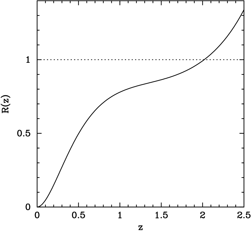
Figure 3: Ratio of the survey flux limit to the characteristic flux of the luminosity function, with parameters chosen to match the SDSS EDR Quasar Catalog.

2.4 Equivalent Width Distribution

The spectral intensity in the vicinity of an emission line is sum of two components, from the continuum and the emission-line region itself:

$$I_{tot}(\lambda)=I_{CR}(\lambda)+I_{BLR}(\lambda).$$ (25)

The equivalent width of an emission line at wavelength $\lambda_{0}$ is defined as the continuum-weighted integral of the line intensity and is quoted in units of wavelength:

$$W=\frac{1}{I_{CR}(\lambda_{0})}\int\left[I_{tot}(\lambda)-I_{CR}(\lambda)\right]d\lambda.$$ (26)

If the continuum region of the quasar is preferentially magnified by a factor $\mu$, then the observed continuum intensity in the above equation becomes $\mu\,I_{CR}(\lambda_{0})$, while the strength of the line itself $I_{BLR}(\lambda)$ remains essentially unchanged. The emission line of a lensed object is thus effectively demagnified with respect to its unlensed width $W_{0}$:

$$W_{\lambda}=\frac{W_{0}}{\mu}.$$ (27)

If $p_{W0}(W_{0})\,dW_{0}$ is the intrinsic distribution of rest-frame equivalent widths, then the observed rest-frame distribution $p_{W}(W_{\lambda})\,dW_{\lambda}$ is:

$$p_{W}(W_{\lambda};z)\,dW_{\lambda}=dW_{\lambda}\int_{0}^{\infty}\mu\,p_{0}(\mu W_{\lambda})\,p_{s}(\mu;z)\,d\mu.$$ (28)

Equations 27 and 28 imply that one would expect an enhanced population of quasars with small equivalent widths if lensing is significant.

To examine the behavior of Equation 28, consider a highly unrealistic $\delta$-function intrinsic equivalent width distribution. The lensing model predictions for a population of emission lines with $W_{0}=20$ Å are plotted in Figure 4 (the functions appear not to be normalized, due to the inability to plot the $\delta$-function at $W=\left\langle{\mu_{u}}\right\rangle W_{0}$ from Equation 11). The low equivalent width signal shown in these plots is a direct consequence of the bias-amplified, high-magnification tail from Equation 23.

Figure 4: Lensed equivalent width distribution, given an intrinsic $\delta$-function distribution, for $\Omega_{c}=0.03$ (solid line) and $\Omega_{c}=0.1$ (dashed line), at redshifts of 1 (top) and 2 (bottom). These plots use the SDSS EDR magnitude limit for quasars.

It is instructive to consider how the lensed distribution is affected by the form of the flux ratio $R(z)$. The value of this function at a given redshift essentially determines the amount of amplification bias. For $R(z)>1$, the survey flux limit is located on a steeper portion of the luminosity function compared to when $R(z)<1$, indicating many more quasars just below the detection threshold that can be lensed into the sample. This leads to an interesting conclusion: by setting the survey flux limit artificially higher, one can expect to see a greater percentage of microlensed quasars. A dramatic illustration of this is shown in Figure 5 for which the survey limit was made 1 mag brighter relative to Figure 4. Every 1 mag change in the survey limit multiplies $R(z)$ by a factor of 2.51; given the EDR and 2dF parameters from before, this means the new flux ratio becomes larger than 1 for $z>0.5$ instead of for $z>2$. The tradeoff, of course, is a reduced number of total observations as well as a smaller average optical depth to lensing for the sample.

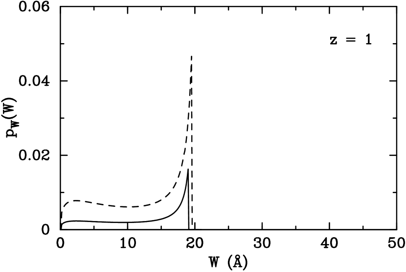
Figure 5: Lensed equivalent width distribution, given an intrinsic $\delta$-function distribution, for $\Omega_{c}=0.03$ (solid line) and $\Omega_{c}=0.1$ (dashed line), again at redshifts of 1 (top) and 2 (bottom). Here the survey flux limit is set 1 mag brighter to demonstrate the effect of amplification bias.

While the $\delta$-function distribution is a useful beginning, a much more realistic model for intrinsic equivalent widths is the lognormal distribution,

$$p_{0}(W_{0})\,dW_{0}=\frac{dW_{0}}{\gamma\,W_{0}\sqrt{2\pi}}e^{-(\ln W_{0}-\omega)^{2}/2\gamma^{2}}.$$ (29)

Here the “shape parameters” $\omega$ and $\gamma$ are the mean and standard deviation, respectively, of $\ln W$. This is largely an empirically determined distribution, although there have been attempts to provide a physical explanation (Francis, 1993). As will be shown in Section 3, the lognormal distribution provides a very good approximation to the actual quasar data. Figure 6 shows how the lensed equivalent width model appears for various values of $z$ and $\Omega_{c}$, and choosing $\omega$ and $\gamma$ as appropriate for the data set. As in Figure 4, there is a clear lensing indicator in the low equivalent width region that scales with both $z$ and $\Omega_{c}$.

Figure 6: Lensed equivalent width distribution, given an intrinsic lognormal distribution, for $\Omega_{c}=0.0$ (solid line), $\Omega_{c}=0.03$ (dashed line), and $\Omega_{c}=0.1$ (dotted line), at redshifts of 1 (top) and 2 (bottom).

Because of the large amount of integration involved in arriving at the final expression (28) for the lensed-lognormal equivalent width distribution, it becomes necessary to compute an interpolated version of the model. Through a change of variables,

$$u(W)=\frac{\ln W-\omega}{\gamma}+\gamma,$$ (30)

it is possible to remove $\omega$ dependence from the integral of the lensed-lognormal model. Then polynomial interpolation of the expression

$$\ln[\gamma\,p_{W}(u(W))]+\omega-\frac{\gamma^{2}}{2}$$ (31)

over the remaining four variables $(u,z,\gamma,\Omega_{c})$ gives a very good fit to the actual distribution. In the $\Omega_{c}=0$ case, Equation 31 is a simple parabola in $u$, independent of all other parameters.

3 Data

This section describes the details of the selection of the equivalent width data set, and addresses concerns regarding the choice of an appropriate sample to be modeled.

3.1 SDSS Early Data Release and Quasar Catalog

The Sloan Digital Sky Survey uses a dedicated 2.5 m telescope at Apache Point Observatory, New Mexico, with an approximate $3^{\circ}$ field of view, to obtain photometric and spectroscopic data at high Galactic latitudes. A CCD mosaic camera (Gunn et al., 1998) obtains imaging data in drift-scan mode for five broad optical photometric bands ($ugriz$) that were designed for the Survey (Fukugita et al., 1996). From the imaging data, up to 640 objects per field are selected for simultaneous observation by a pair of fiber-optic spectrographs covering the range from 3800 Å to 9200 Å. In addition, an auxiliary 20 inch (0.5 m) Photometric Telescope at the site provides photometric calibrations (see York et al. 2000 for more details).

The Early Data Release (EDR) (Stoughton et al., 2002) consists of 462 square degrees of imaging data from eight drift scans, and 54,008 individual spectra. The data were acquired along the celestial Equator in both the northern and southern Galactic skies, with additional fields corresponding to a portion of the SIRTF First Look Survey region. This first public data release represents only a fraction of the planned survey coverage of the northern ($10^{4}$ deg²) and southern ($\sim 750$ deg²) Galactic caps. Because the SDSS photometric system was not finalized at the time of the public data release, the EDR photometry is referred to here as (${u^{\ast}}{g^{\ast}}{r^{\ast}}{i^{\ast}}{z^{\ast}}$).

SDSS quasar candidates are selected from photometric data using a sophisticated multicolor algorithm (see Richards et al. 2002a for details). Candidates for follow-up spectroscopy must also meet PSF ${i^{\ast}}$ magnitude requirements. There is a bright cutoff of ${i^{\ast}}>15.0$ to prevent brighter objects’ spectra from bleeding into adjacent spectra on the CCD detector. A Galactic extinction-corrected faint cutoff of ${i^{\ast}}<19.1$ (for $z\lesssim 3$ quasars) flux-limits the multicolor sample; this limit was chosen to satisfy catalog completeness requirements given the sky density of quasars and the number of fibers allocated to quasars per spectroscopic plate. Of course, high-redshift quasars and those targeted by other means (e.g., serendipity) may be fainter than this limit. One important caveat is that the EDR employed earlier versions of the quasar targeting algorithm for its commissioning data, slightly modifying the magnitude limits. In particular, two of the image processing runs have a bright cutoff at ${i^{\ast}}=16.5$ (the remainder use ${i^{\ast}}=15.0$), and for all EDR data the faint dereddened limit is ${i^{\ast}}<19.0$.

The first edition of the SDSS Quasar Catalog (Schneider et al., 2002), based on the EDR, includes 3814 objects, 3000 of which were discovered by the SDSS. Quasars with reliable redshifts were selected for inclusion in the catalog if their spectra contained at least one broad emission line (FWHM $>1000$ km s^-1) and their luminosity exceeded $M_{{i^{\ast}}}=-23$ (calculated in a $H_{0}=50$ km s^-1 Mpc^-1, $\Omega_{M}=1.0$, $\Omega_{\Lambda}=0.0$ cosmology). The quasars range in redshift from 0.15 to 5.03. It is expected that the final SDSS Quasar Catalog will contain on the order of $10^{5}$ quasars. A few sample spectra from the catalog are presented in Figure 7.

Figure 7: Sample quasar spectra at moderate redshift from the EDR, illustrating large equivalent widths in all three lines (top), a bright quasar (middle), and very low equivalent widths in all three lines (bottom). The last quasar is a good microlens candidate.

3.2 Creation of Equivalent Width Samples

For the purposes of this paper, I examined the strong Mg ii, C iii], and C iv broad emission lines from EDR quasars. The first step was to extract information from the SDSS Catalog Archive using the SDSS Query Tool. I selected all measured spectral lines belonging to objects classified as quasars, and for which the redshift measurements were not deemed to be of low confidence. A sample query for the Mg ii line, in SQL notation, is

  SELECT spec.plate.plateID, spec.plate.mjd, spec.fiberID
  FROM sxSpecLine
  WHERE (category == 1 && name.lineID == 2800 &&
    (spec.specClass == SPEC_QSO || spec.specClass == SPEC_HIZ_QSO) &&
    (spec.zWarning & Z_WARNING_LOC) == 0)

This first set of queries resulted in 2809 Mg ii lines, 2295 C iii] lines, and 1650 C iv lines, from a total of 3280 spectroscopic observations classified as quasars in the EDR. (Without the low-confidence redshift constraint, these numbers are 3368, 2738, and 1909 respectively, from 3925 quasars.)

Next, I removed from the results of the Archive queries all objects that did not appear in the official SDSS Quasar Catalog. This reduced the number of distinct quasars to 3095 (2637 Mg ii lines, 2215 C iii] lines, and 1595 C iv lines). There are 130 objects in the Quasar Catalog not tagged as low-confidence that do not appear in the any of catalogs returned by the SQL queries. Of these, the vast majority have redshifts either too small or too large for the spectral lines of interest to appear in the spectroscopic data. The remainder include 7 of the 10 objects added to the catalog from a visual inspection of EDR spectra, and 14 of the 16 objects added during a visual search for extreme broad absorption-line (BAL) quasars.

Spectral line parameters are determined by fitting a single Gaussian to the continuum-subtracted flux in the neighborhood of an identified line. Several entries in the Catalog Archive describe the quality of the spectral line fits. In particular, I considered the fractional error of the equivalent width, $\sigma_{W}/W$ (calculated from the uncertainties in the fit parameters), and the chi-squared per degree of freedom for the fit, $\chi^{2}/\nu$. Histograms of these parameters for each data set are shown in Figures 8 and 9. There are anomalous spikes in the equivalent width fractional error histograms just above 0.5 and again at 0.9, for reasons that remain unclear.

Figure 8: Histograms of equivalent width fractional error for Mg ii, C iii], and C iv respectively.

Figure 9: Histograms of $\chi^{2}/\nu$ for Mg ii, C iii], and C iv respectively.

Based on these histograms, I chose a reasonable absolute minimum “data quality” standard of $\sigma_{W}/W\leq 0.5$, $\chi^{2}/\nu\leq 5.0$, with an additional requirement that the equivalent width itself be a positive number. In Section 4 I consider the effect that more restrictive data quality cuts in $\sigma_{W}/W$ and $\chi^{2}/\nu$ have on the constraints placed on $\Omega_{c}$. This reduced the data set to 2333 Mg ii lines, 1929 C iii] lines, and 1322 C iv lines. I then visually inspected all spectral lines and their fits, eliminating observations with poor fits due to large nearby absorption systems, excessive noise from atmospheric lines, and other examples of poor fitting on the part of the spectroscopic pipeline algorithms; see Figure 10 for sample line fits. In general I opted to keep truly borderline observations, reasoning that these data would tend to make the bounds on $\Omega_{c}$ more conservative, and also with the knowledge that many such borderline objects would be eliminated automatically by stricter data quality cuts. In all, 99 Mg ii lines, 61 C iii] lines, and 61 C iv lines were removed from the data sample based on visual inspection.

Figure 10: Examples of good (top) and poor (bottom) Gaussian line fits to Mg ii. Each plot shows the best fit to the continuum-subtracted flux, with the error displayed beneath. The line in the bottom plot is marred by an absorption system.

Finally, based on the redshift limits of the 2dF luminosity function ($z\leq 2.3$), and the quasar targeting algorithm faint limit (dereddened ${i^{\ast}}<19.0$), I obtain 1857 Mg ii equivalent widths with $0.36<z<2.21$, 1382 C iii] observations with $1.01<z<2.3$, and 745 C iv equivalent widths with $1.47<z<2.3$. Figures 11 and 12 show the number of observations of each line binned by redshift and dereddened ${i^{\ast}}$ apparent magnitude.

Figure 11: Histogram of redshift for each spectral line, as well as for all quasars in the sample.

Figure 12: Histogram of dereddened ${i^{\ast}}$ magnitude for each spectral line, as well as for all quasars in the sample.

3.3 Appropriateness of Sample

There are several important considerations that apply to the choice of quasar sample for this test. One central assumption in the development of the equivalent width model distribution is that the sample is continuum flux-limited, in order that amplification bias may be treated correctly. Optically selected samples such as the SDSS Quasar Catalog will not be exactly limited by continuum flux due to contributions from line emission. Because the sample is limited by ${i^{\ast}}$ magnitude, the Mg ii line will contribute to the measured filter flux for quasars with redshifts $1.4<z<1.9$ (Fukugita et al., 1996); the C iii] and C iv lines not appear in $i$ over the redshifts studied, although other lines such as [O iii] and some of the Balmer series do move into the $i$ filter at low redshift. However, the width of the filter is about 1200Å while the typical observed emission line equivalent width is less than 10% of this, so the typical magnitude in this situation will be less than $0.1$ brighter than the continuum-only value.

It is also important for the sample to be as complete as possible. The SDSS quasar targeting algorithm (Richards et al., 2002a) has been shown to be at least 90% complete for $z<2.5$ and ${i^{\ast}}<19.1$ (19.0 for the EDR). Since the luminosity function is only determined for $z<2.3$ (Boyle et al., 2000), completeness in redshift is not a concern. The Quasar Catalog absolute magnitude limit of $M_{i^{\ast}}=-23$ does not in practice affect the sample either. As shown in Figure 3 of Schneider et al. (2002), this restriction removes only Mg ii observations near ${i^{\ast}}=19.0$ with $z<0.42$, a negligibly small population that is highly unlikely to exhibit microlensing. The Quasar Catalog requirement that FWHM $>1000$ km s^-1 for at least one emission line is more worrisome, since this may exclude small equivalent width observations. On the other hand, this criterion was chosen specifically to eliminate narrow-lined quasars, which don’t belong in a study of the broad emission line region. Moreover, only 10 quasars were dropped from the catalog based solely on this criterion. Finally, the bright-limit discrepancy (${i^{\ast}}=15.0$ versus ${i^{\ast}}=16.5$) in different EDR processing runs affects only a very few observations, as can be seen from the relative paucity of bright quasars in Figure 12.

3.3.1 Emission Lines

The microlensing signature in the equivalent width distribution depends on the fact that a broad emission line arises from a much larger region than does the continuum surrounding it in the spectrum. Although Mg ii can be considered the most useful emission line due to both the wide range of redshift and sheer numbers, it suffers from being located in the midst of what has been termed the “small blue bump.” What appears to be a slightly brighter region of the rest-frame continuum from 2000-3600Å is in fact the continuum plus blended Fe ii multiplets and high-order Balmer series lines (Wills et al., 1985). If the Mg ii equivalent width is calculated relative to this false high continuum (as in the SDSS spectroscopic pipeline), any magnification of the true continuum due to lensing will be underestimated. The composite SDSS quasar spectrum of Vanden Berk et al. (2001) suggests that the contribution of line emission to the apparent continuum around Mg ii is on the order of 25-50%. Thus high-magnification lensing events might appear to have an effective magnification only $2/3$ the actual value. This would tend to dilute the lensing signal, leading to overly optimistic constraints on $\Omega_{c}$.

The C iii] and C iv lines do not share the continuum problems of Mg ii. Because they enter the optical region at higher redshifts, however, they lack the advantage of a long redshift baseline. There are also necessarily fewer observations in the flux-limited sample. C iii] does have one edge over the others; line variability studies suggest that C iii] may be emitted from larger regions of the quasar than other lines (Peterson, 1997).

3.3.2 Time Dependence of Microlensing

While the characteristic time dependence of microlensing is the key to many of its applications, such is not the case with this method. It is important that the spectroscopic observations not lag far behind the photometric imaging. If this delay is too large, the microlensing event that may have amplified a quasar into the flux-limited sample will have ended, and the equivalent widths will no longer reflect the fact that the quasar was once lensed. To estimate the decorrelation timescale, consider the time it takes for a lens moving with velocity $v_{\perp}$ (perpendicular to the line of sight) to cover a distance equal to its Einstein radius (Schneider et al., 1992):

$$\Delta t=\frac{\alpha_{E}D_{L}}{v_{\perp}}\approx 78h^{-1/2}\left(\frac{300\mbox{ km s${}^{-1}$}}{v_{\perp}}\right)\left(\frac{M}{M_{\sun}}\right)^{1/2}\mbox{yr},$$ (32)

where $v_{rel}$ is the velocity of the lens perpendicular to the line of sight. For a conservative estimate of a $0.001M_{\sun}$ lens with a velocity dispersion of $300$ km s^-1, this timescale is only 2.9 yr.

To address this concern, I queried the SDSS Catalog Archive for the MJD of the spectroscopic and photometric observations of the quasars. The median time delay between observations was 1.9 yr, with a minimum of just 0.14 yr and a maximum of 2.3 yr; Figure 13 shows a histogram of the time delays. While these time differences are smaller than the timescale estimate above, they are a potential source of worry for the EDR data. It is however important to note that an order of magnitude larger lens mass pads the decorrelation timescale by a comfortable factor of 3. Moreover, because the quasar survey flux limit is for the most part less than the characteristic flux of the luminosity function (see Figure 3), the amplification bias is correspondingly weaker than if the flux limit resided on the steep power-law slope of the LF. The fewer observations there are due to bias, the less the decorrelation between photometric and spectroscopic measurements matters.

Figure 13: Difference in MJD between photometric and spectroscopic observations for EDR quasars.

3.3.3 Other Quasar Samples

The first EDR-based SDSS Quasar Catalog is by no means the only flux-limited sample available, nor is it the largest. The Large Bright Quasar Survey (Hewett, Foltz, & Chaffee, 1995) set the standard for the current era of massive spectroscopic surveys, containing approximately 1/4 the number of quasars in the EDR. The 2dF collaboration has far surpassed both with a publicly released spectroscopic catalog of $10^{4}$ quasars (Croom et al., 2001), and will soon release the full catalog of nearly 24,000 quasars. The SDSS also very recently announced its “beta version” of Data Release 1, containing 17,700 quasar spectra with $z<2.3$.

Despite the smaller size, the EDR Quasar Catalog edges out the 2dF catalog in several ways. The SDSS spectrograph obtains data to longer wavelengths (9200 Å compared to 2dF’s 7900 Å limit), allowing higher redshift observations of the Mg ii line in particular. The SDSS catalog is also 90% complete to a slightly higher redshift than 2dF. Perhaps most importantly, the SDSS spectroscopic data-processing pipeline produces as a matter of course a wealth of information characterizing the spectra and their emission lines.

4 Analysis

This section describes the use of the maximum-likelihood method for determining the bounds on $\Omega_{c}$. Given a probability distribution of equivalent widths (Equation 28), the logarithm of the likelihood function may be written generically as

$$\ln L(W_{i};z_{i},\theta)=\sum_{i}\ln p_{W}(W_{i};z_{i},\theta),$$ (33)

where $\theta$ represents the parameter collection. So far in the discussion of the lensed equivalent width distribution, the parameters consist of $(\Omega_{c},\omega,\gamma)$ (i.e., the compact dark matter fraction plus the two shape parameters of the intrinsic lognormal distribution). Also implicit in this list from consideration of the extended source is $M_{lens}$; this parameter will be treated separately below.

Figure 14 shows the equivalent width distributions for the three sets of emission line data constructed in Section 3. Also plotted are the best-fit lognormal distribution for each data set. These plots clearly demonstrate that the model assumption of lognormality is well-motivated.

Figure 14: Equivalent width histograms for Mg ii (top), C iii] (middle), and C iv (bottom) data sets, along with their best-fit lognormals.

One might worry that more restrictive “data quality” standards than those imposed in Section 3.2 (such as are considered below) would tend to bias the data strongly for or against evidence of lensing. If that were the case, a histogram of the equivalent widths culled by the new requirement ought to show evidence of being skewed toward high or low values. Figure 15 shows those data removed by the criteria $\sigma_{W}/W\leq 0.4$ and $\chi^{2}/\nu\leq 3.0$. There is no indication from these histograms of obvious bias in the selection criteria.

Figure 15: Equivalent width histograms for the data culled by the criteria $\sigma_{W}/W\leq 0.4$ and $\chi^{2}/\nu\leq 3.0$. Once again, Mg ii is on top, followed by C iii] and C iv.

It is also instructive to divide the equivalent width data into different redshift ranges, looking for obvious signs of microlensing. Figure 16 shows this for the Mg ii observations. It is immediately evident by comparing these histograms to the models in Figure 6 that the lensing effect, if any, is quite small. There is no apparent sign of an enhanced fraction of low equivalent width quasars that appears to increase with redshift.

Figure 16: Equivalent width histograms for Mg ii, for different redshift ranges.

4.1 Baldwin Effect

Unfortunately, as Figure 16 illustrates, the universe is not so kind as to oblige with a non-evolving intrinsic equivalent width distribution requiring only two parameters. In fact, using just the three parameters $(\Omega_{c},\omega,\gamma)$ listed above yields a very poor fit to the EDR quasar data, as measured by a $\chi^{2}$ statistic ($\chi^{2}/\nu\gtrsim 2.3$ for Mg ii). The difficulty is due to a phenomenon known the Baldwin effect, in which the equivalent width of many quasar broad emission lines is anti-correlated with luminosity (Baldwin, 1977; Croom et al., 2002) or perhaps, as some have suggested, with redshift (Green, Forster, & Kuraszkiewicz, 2001).

While Figure 16 would seem to indicate a redshift-dependent evolution of the equivalent width distribution, this could be a result of the fact that higher redshift quasars in a flux-limited sample will tend to have higher luminosity. Figure 17 shows histograms of the observations in different ranges of absolute magnitude in ${i^{\ast}}$, and suggests a similar trend.

Figure 17: Equivalent width histograms for Mg ii, for different absolute magnitude ranges.

The purpose of the present work is not to characterize the Baldwin effect in great detail; however, some basic understanding is needed to account for this evolution effect in the likelihood function. To elucidate whether the $z$ or $M_{i^{\ast}}$ correlation might be stronger, I again divided the observations into redshift or magnitude bins, and calculated the mean and standard deviation of $\ln W$ for each bin (equivalently yielding $\omega$ and $\gamma$ for the best-fit unlensed lognormal distribution). The results for each of the three emission lines are plotted in Figures 18–20. These plots suggest that the variation is correlated more strongly with $M_{i^{\ast}}$.

Figure 18: Mean (top) and standard deviation (bottom) of $\ln W$, versus redshift (left) or absolute magnitude (right), for Mg ii.

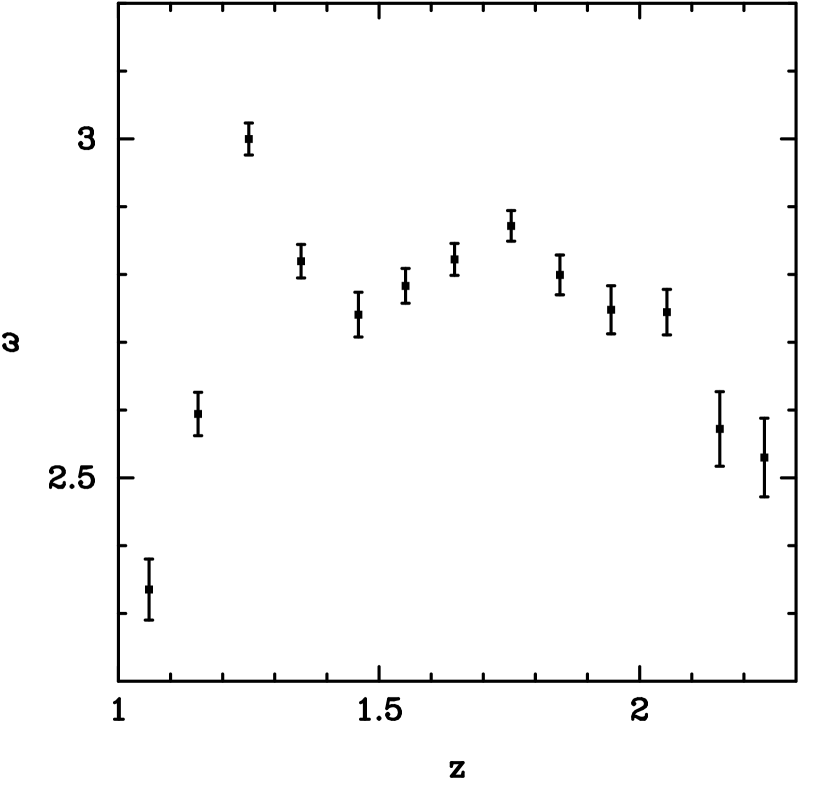
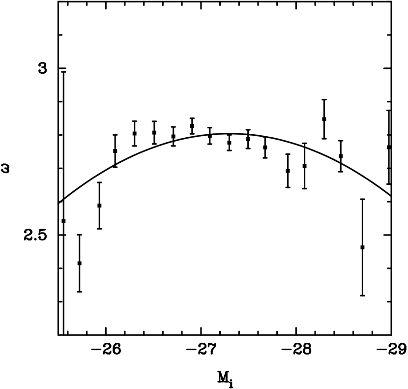
Figure 19: Mean (top) and standard deviation (bottom) of $\ln W$, versus redshift (left) or absolute magnitude (right), for C iii].

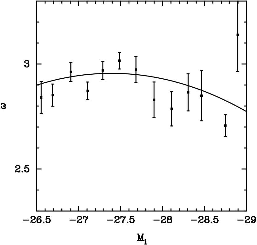
Figure 20: Mean (top) and standard deviation (bottom) of $\ln W$, versus redshift (left) or absolute magnitude (right), for C iv.

In the absence of an obvious linear relationship for most cases, I allow the shape parameters to vary with magnitude as follows:

$$\omega_{MgII}(M) = \omega_{0}+\omega_{1}(M-M_{0})\mbox{ for $M<M_{0}$ ($\omega_{0}$ otherwise)}$$

$$\gamma_{MgII}(M) = \gamma_{0}+\gamma_{1}(M-M_{0})$$

$$\omega_{CIII}(M) = \omega_{0}+\omega_{1}(M-M_{0})^{2}$$ (34)

$$\gamma_{CIII}(M) = \gamma_{0}+\gamma_{1}(M-M_{0})^{2}$$

$$\omega_{CIV}(M) = \omega_{0}+\omega_{1}(M-M_{0})^{2}$$

$$\gamma_{CIV}(M) = \gamma_{0}+\gamma_{1}(M-M_{0})^{2}.$$

The sets of parameters $(M_{0},\omega_{0},\omega_{1},\gamma_{0},\gamma_{1})$ are of course fit separately for each data set. There is no real a priori justification for keeping the characteristic magnitude parameters $M_{0}$ the same for both the $\omega$ and $\gamma$ fits, other than to reduce the number of parameters being added to the likelihood function.

4.2 Equivalent Width Fractional Error

Each measurement of equivalent width in the quasar catalog $W_{i}$ is accompanied by an estimate of the measurement error $\sigma_{W,i}$. In principle these errors can be incorporated into the likelihood function; for example, if the errors are assumed to be normal, then for each data point Equation 28 can be convolved with a Gaussian with a width equal to the fractional error $\sigma_{W,i}/W_{i}$. When there is no lensing, this is approximately equivalent to adding the fractional error in quadrature to the lognormal width parameter $\gamma$. This leads to slightly smaller determinations of the best-fit $\gamma$, on the order of $0.02$ for the EDR data, and also tends to shift the best-fit $\omega$ systematically higher. The non-zero $\Omega_{c}$ case is considerably more difficult to treat in the maximum-likelihood formulation. However, for small $\Omega_{c}$ and typical values of the lognormal shape parameters, and given that typically $\sigma_{W,i}/W_{i}\lesssim 0.2$ for the observations, it can be seen that the convolved distribution, though slightly wider, does not differ appreciably in the strength of the low equivalent width lensing signature, so estimates of $\Omega_{c}$ will not be significantly affected. Additionally, since the intrinsic values of the lognormal shape parameters are not of interest here, and because accounting for equivalent width measuring error takes vastly more CPU time, I disregard this contribution.

4.3 Maximum-Likelihood Analysis

For each spectral line data set, and using a model in which $M_{lens}=1M_{\sun}$ I maximized the log-likelihood function, allowing $\Omega_{c}$ to be the undetermined parameter and marginalizing over all others. In an attempt to determine how the quality of the line fits affects the results, I made three different “data quality” cuts, requiring ($\sigma_{W}/W$, $\chi^{2}/\nu$) to be less than (0.5, 5.0), (0.4, 3.0), or (0.3, 2.0) for “minimal,” “intermediate,” and “strict” cuts. Results, normalized to a common maximum-likelihood value, are shown in Figure 21. The 95% confidence level is attained in this one-parameter case when $\ln L=\ln L_{max}-1.92$ (Cowan, 1998). It is perhaps somewhat surprising that weakening the data selection criteria do not always produce more conservative limits for $\Omega_{c}$.

Figure 21: Maximized log-likelihood versus $\Omega_{c}$ for each data set, using a model with $M_{lens}=1M_{\sun}$. The lines represent the minimal (solid line), intermediate (dashed line), and strict (dotted line) data quality cuts.

I also consider a $M_{lens}=0.001M_{\sun}$ lensing model for each of the three samples of lines, using the “intermediate” selection criteria for the data. The maximum-likelihood curves for all three lines are plotted together in Figure 22. The limits from this plot, along with those from the $1M_{\sun}$ lens model, are summarized in Table 1.

Figure 22: Maximized log-likelihood versus $\Omega_{c}$ in a $M_{lens}=0.001M_{\sun}$ model, for all three data sets. The lines represent Mg ii (solid line), C iii] (dashed line), and C iv (dotted line) data sets.

Goodness of fit can be measured with a $\chi^{2}$ statistic applied to the binned data sets. For the various combinations of the three emission lines and the two lens masses, $\chi^{2}/\nu$ values range from 1.2 to 1.6, indicating that the model represents a generally acceptable fit.

4.4 Tests of Maxmimum-Likelihood Method

Applying the maximum-likelihood analysis to some simple modifications of the data set serves as an indication of the method’s validity and sensitivity. For example, one expects that adding or removing low equivalent width, high redshift observations will increase or decrease respectively the maximum-likelihood estimator (MLE) of $\Omega_{c}$ or its upper bound. In one such test, I removed the lowest four equivalent widths (0.4% of the data set) from the C iii] “intermediate quality” data set; the widths ranged from 2.3 Å to 4.3 Å and were at redshifts of 1.1, 1.5, 1.8, and 2.2. This modification shifted the 95% confidence upper limit on $\Omega_{c}$ from 0.022 to 0.02; while the MLE value of $\Omega_{c}$ remained virtually unchanged, the peak was considerably flattened and the lower bound moved from 0.006 to 0.002. In a similar test, adding just four counterfeit low equivalent widths (from 2.0 Å to 2.4 Å) to the original data set, at moderately high redshift ($z=1.6$ to $2.0$), was sufficient to shift the upper limit to 0.028 and $\Omega_{c,MLE}$ from 0.015 to 0.018.

I also tested how well the maximum-likelihood method could determine $\Omega_{c}$ from synthesized data sets. Keeping each C iii] redshift and magnitude measurement the same, I replaced the equivalent widths with Monte Carlo “data” generated using the magnitude-dependent lognormal shape parameters from the actual data set, and assuming $\Omega_{c}=0.03$. The analysis of this fake data appropriately yielded $\Omega_{c,MLE}=0.032$ with an upper bound of 0.045. For a lens-free $\Omega_{c}=0$ synthetic data set, the maximum-likelihood method correctly produced a peak at $\Omega_{c,MLE}=0$ with an upper limit of 0.007.

4.5 Scaling to Larger Samples

Anticipating the growth in the SDSS quasar catalog, I have made an attempt to estimate how the constraints on $\Omega_{c}$ depend on the number of equivalent widths measured. From the Mg ii data set I generated random subsamples of various sizes (as well as one supersample using sampling with replacement), and performed the same maximum-likelihood analysis in each case. The results are plotted as log-limit versus log-number in Figure 23. The slope of the fit is $-0.56$, indicating that the bound on $\Omega_{c}$ scales approximately like $1/\sqrt{N}$. This makes sense in light of the fact that the fraction of low equivalent width lines in the lensing model (i.e., the lensing signal divided by $N$) scales roughly linearly with $\Omega_{c}$ for $\Omega_{c}\ll 1$. Because the EDR Quasar Catalog represents about 4% of the SDSS goal for quasar observations, this implies it may be possible to improve the constraints by a factor of 5.

Figure 23: $\sigma_{\Omega_{c}}$ versus $N$ for Monte Carlo samples from the Mg ii data set.

5 Conclusions

I have shown that microlensing by cosmologically distributed compact objects in the mass range $0.001$–$1M_{\sun}$ can produce a detectable increase in the fraction of small equivalent width quasar emission lines with redshift. Table 1 details the limits derived from each emission line studied and assuming lens masses at either extreme of the range. To summarize these results, and based on the lack of a strong lensing signal, $\Omega_{c}$ is constrained to be less than approximately $0.03$ at 95% confidence over this mass range.

Table 1: Upper limits (95% confidence level) on cosmological compact dark matter.

Spectral Line	$M_{lens}=1M_{\sun}$	$M_{lens}=0.001M_{\sun}$
Mg ii	$\Omega_{c}<0.014$	$\Omega_{c}<0.024$
C iii]	$\Omega_{c}<0.025$	$\Omega_{c}<0.031$
C iv	$\Omega_{c}<0.029$	$\Omega_{c}<0.047$

This limit is interesting in several respects. First of all, it is stricter than limits derived from the current microlensing searches within our own halo (e.g., Alcock et al. 2000a); if at most one-third of the Galactic halo mass is compact, then their results imply $\Omega_{c}\lesssim 0.1$ for $\Omega_{M}=0.3$. Additionally, since $\Omega_{c}<\Omega_{B}\approx 0.04$, it may not ultimately be necessary to invoke exotic non-baryonic compact objects to explain microlensing events. This conclusion will be made much stronger if larger future quasar samples demonstrate the limit on $\Omega_{c}$ to be $\lesssim 0.01$, the fraction of baryons unexplained in the current census (Silk, 2003). Also below this threshold, microlensing by ordinary stars in galaxies may become more significant, since $\Omega_{\ast}\approx 0.006$ (Fukugita, Hogan, & Peebles, 1998).

There are some important points to keep in mind when considering the analysis leading to these constraints. The first is that, because the three sets of emission lines are from only one sample of quasars, the constraints are not independent and cannot in general be combined to derive a stronger limit. Rather the three sets of limits serve in some sense as checks on one another. The second point concerns the absence of quoted lower limits. While the maximum-likelihood analysis formally produces a nonzero most-likely value for $\Omega_{c}$ in some cases, along with a lower limit, this should not be interpreted as an unambiguous detection of compact dark matter. It may very well be that the intrinsic distribution at low equivalent widths departs from a simple lognormal; this could be easily be misconstrued as evidence for lensing at low $\Omega_{c}$. Another way of saying this is that because probability must be non-negative, any departure from the exponentially small intrinsic probability at low equivalent width will result in a positive detection of compact dark matter, real or not. The other side of this argument is that if the actual unlensed distribution does in fact have some probability at low equivalent widths not represented in the model, then the limits from the simple lognormal-based model will necessarily be conservative.

A large source of systematic uncertainty in this analysis is the Baldwin effect, which deserves a much more thorough treatment than was possible in this paper. The maximum-likelihood requirements of an adequately parameterized distribution has led to the introduction of a number of ad hoc parameters irrelevant to the final result. Much work remains to be done in characterizing the luminosity evolution of equivalent width. It would also be worthwhile to consider alternate methods of constructing statistics for determining $\Omega_{c}$ that would rely less on knowing the details of the Baldwin effect while still using the sheer numbers of observations to full advantage.

An additional source of systematic error is the single-component Gaussian line-fitting process in the SDSS spectroscopic pipeline. Quasar broad emission lines are often fit more closely by using an additional Gaussian to incorporate the flux in the broad low wings. Even this can fail to account fully for the wavelength shifts and line asymmetries often found in quasar spectra (Richards et al., 2002b). Some recent work within the SDSS Collaboration has focused on improving the current quasar line fitting algorithm .

The lensing model is another area in which much improvement can be made. The assumption of uniformly distributed cosmological lenses in the spirit of Press & Gunn (1973), although analytically simple, is violated by the clustering actually observed in the universe. While Dalcanton et al. (1994) convincingly argue that compact object correlations are unimportant for the relatively small lensing optical depths under consideration, Wyithe & Turner (2002) suggest that lens clustering in galactic dark matter halos might decrease the fraction of microlensed sources (and hence weakening the constraints on $\Omega_{c}$) by as much as a factor of two. Moreover, the overall magnification distribution can be altered by considering the effects of smooth dark matter in halos, in which the compact lens may reside. Perna & Loeb (1998) examine the possibility of using this quasar equivalent width method to detect the signature of extragalactic halo MACHOs in the final SDSS quasar catalog. Mörtsell, Goobar, & Bergström (2001) and Metcalf & Silk (1999) consider models with both smooth and compact dark matter components in the context of lensed Type Ia supernovae. Seljak & Holz (1999) have also made predictions for SNe Ia lensing by incorporating large scale structure information from N-body simulations.

Finally, the data set itself will only become more powerful as the SDSS continues to increase its tally of spectroscopically observed quasars. When the SDSS quasar luminosity function is determined, it will remove the mismatch between $B$ and $i$ magnitudes that is a concern with the current use of the 2dF luminosity function. The large quasar sample will also permit a much more detailed characterization of emission line properties that will hopefully lead to a better understanding of quasar structure, and hence of the effects of quasar microlensing.

References

- Alcock et al. (2000a) Alcock, C. et al. 2000a, ApJ, 542, 281
- Alcock et al. (2000b) —. 2000b, ApJ, 541, 734
- Baldwin (1977) Baldwin, J. A. 1977, ApJ, 214, 679
- Banerjee et al. (2003) Banerjee, S., Bhattacharyya, A., Ghosh, S. K., Raha, S., Sinha, B., & Toki, H. 2003, MNRAS, 340, 284
- Bennett et al. (2003) Bennett, C. L. et al. 2003, ApJ, in press (astro-ph/0302207)
- Boyle et al. (2000) Boyle, B. J., Shanks, T., Croom, S. M., Smith, R. J., Miller, L., Loaring, N., & Heymans, C. 2000, MNRAS, 317, 1014
- Burles et al. (2001) Burles, S., Nollett, K. M., & Turner, M. S. 2001, ApJ, 552, L1
- Canizares (1982) Canizares, C. R. 1982, ApJ, 263, 508
- Cowan (1998) Cowan, G. 1998, Statistical Data Analysis (Oxford: Clarendon Press)
- Croom et al. (2002) Croom, S. M. et al. 2002, MNRAS, 337, 275
- Croom et al. (2001) Croom, S. M., Smith, R. J., Boyle, B. J., Shanks, T., Loaring, N. S., Miller, L., & Lewis, I. J. 2001, MNRAS, 322, L29
- Dalcanton et al. (1994) Dalcanton, J. J., Canizares, C. R., Granados, A., Steidel, C. C., & Stocke, J. T. 1994, ApJ, 424, 550
- Dyer & Roeder (1973) Dyer, C. C., & Roeder, R. C. 1973, ApJ, 180, L31
- Fan et al. (2001) Fan, X. et al. 2001, AJ, 121, 54
- Francis (1993) Francis, P. J. 1993, ApJ, 405, 119
- Fukugita et al. (1998) Fukugita, M., Hogan, C. J., & Peebles, P. J. E. 1998, ApJ, 503, 518
- Fukugita et al. (1996) Fukugita, M., Ichikawa, T., Gunn, J. E., Doi, M., Shimasaku, K., & Schneider, D. P. 1996, AJ, 111, 1748
- Gondhalekar (1990) Gondhalekar, P. M. 1990, MNRAS, 243, 443
- Gradshteyn & Ryzhik (1994) Gradshteyn, I. S., & Ryzhik, I. M. 1994, Table of Integrals, Series and Products, 5th edn. (New York: Academic Press)
- Green et al. (2001) Green, P. J., Forster, K., & Kuraszkiewicz, J. 2001, ApJ, 556, 727
- Gunn et al. (1998) Gunn, J. E. et al. 1998, AJ, 116, 3040
- Hewett et al. (1995) Hewett, P. C., Foltz, C. B., & Chaffee, F. H. 1995, AJ, 109, 1498
- Jedamzik (1997) Jedamzik, K. 1997, Phys. Rev. D, 55, 5871
- Lasserre et al. (2000) Lasserre, T. et al. 2000, A&A, 355, L39
- Mörtsell et al. (2001) Mörtsell, E., Goobar, A., & Bergström, L. 2001, ApJ, 559, 53
- Marani et al. (1999) Marani, G. F., Nemiroff, R. J., Norris, J. P., Hurley, K., & Bonnell, J. T. 1999, ApJ, 512, L13
- Metcalf & Silk (1999) Metcalf, R. B., & Silk, J. 1999, ApJ, 519, L1
- Peacock (1999) Peacock, J. A. 1999, Cosmological Physics (Cambridge: Cambridge University Press)
- Pei (1993) Pei, Y. C. 1993, ApJ, 403, 7
- Perna & Loeb (1998) Perna, R., & Loeb, A. 1998, ApJ, 493, 523
- Peterson (1997) Peterson, B. M. 1997, An Introduction to Active Galactic Nuclei (Cambridge: Cambridge University Press), 238
- Press & Gunn (1973) Press, W. H., & Gunn, J. E. 1973, ApJ, 185, 397
- Richards et al. (2002a) Richards, G. T. et al. 2002a, AJ, 123, 2945
- Richards et al. (2002b) Richards, G. T., Vanden Berk, D. E., Reichard, T. A., Hall, P. B., Schneider, D. P., SubbaRao, M., Thakar, A. R., & York, D. G. 2002b, AJ, 124, 1
- Schneider et al. (2002) Schneider, D. P. et al. 2002, AJ, 123, 567
- Schneider (1987) Schneider, P. 1987, A&A, 179, 71
- Schneider (1993) —. 1993, A&A, 279, 1
- Schneider et al. (1992) Schneider, P., Ehlers, J., & Falco, E. E. 1992, Gravitational Lenses (New York: Springer-Verlag)
- Seljak & Holz (1999) Seljak, U., & Holz, D. E. 1999, A&A, 351, L10
- Shalyapin (2001) Shalyapin, V. N. 2001, Astronomy Letters, 27, 150
- Silk (2003) Silk, J. 2003, MNRAS, in press (astro-ph/0212068)
- Stoughton et al. (2002) Stoughton, C. et al. 2002, AJ, 123, 485
- Vanden Berk et al. (2001) Vanden Berk, D. E. et al. 2001, AJ, 122, 549
- Vietri & Ostriker (1983) Vietri, M., & Ostriker, J. P. 1983, ApJ, 267, 488
- Weinberg (1976) Weinberg, S. 1976, ApJ, 208, L1
- Wills et al. (1985) Wills, B. J., Netzer, H., & Wills, D. 1985, ApJ, 288, 94
- Woźniak et al. (2000) Woźniak, P. R., Udalski, A., Szymański, M., Kubiak, M., Pietrzyński, G., Soszyński, I., & Żebruń, K. 2000, ApJ, 540, L65
- Wyithe & Turner (2002) Wyithe, J. S. B., & Turner, E. L. 2002, ApJ, 567, 18
- York et al. (2000) York, D. G. et al. 2000, AJ, 120, 1579
- Zackrisson & Bergvall (2003) Zackrisson, E., & Bergvall, N. 2003, A&A, 399, 23