astro-ph/0307463

UFIFT-HEP-03-16

CRETE-03-13

IMPROVED ESTIMATES OF COSMOLOGICAL PERTURBATIONS

N. C. Tsamis^†

Department of Physics, University of Crete
GR-710 03 Heraklion, HELLAS.

R. P. Woodard^‡

Department of Physics, University of Florida
Gainesville, FL 32611, UNITED STATES.

ABSTRACT

We recently derived exact solutions for the scalar, vector, and tensor mode functions of a single, minimally coupled scalar plus gravity in an arbitrary homogeneous and isotropic background. These solutions are applied to obtain improved estimates for the primordial scalar and tensor power spectra of anisotropies in the cosmic microwave background.

PACS numbers: 04.30.Nk, 04.62.+v, 98.80.Cq, 98.80.Hw

^† e-mail: tsamis@physics.uoc.gr

^‡ e-mail: woodard@phys.ufl.edu

1 Introduction

Mukhanov and Chibisov [1] were the first to suggest that quantum fluctuations during inflation produced the tiny inhomogeneities needed to form the various cosmic structures we observe currently – as the result of gravitational collapse over the course of more than 10 billion years. Early work on the subject was also done by Hawking [2], by Guth and Pi [3], and by Starobinskiĭ [4]. The formalism has since been described at length in a number of review articles [5, 6, 7]. It has received much attention recently owing to the unprecedented precision with which the imprint of these fluctuations on the cosmic microwave background radiation has been imaged by the WMAP satellite [8, 9].

Much of the fascinating structure revealed by these measurements derives from processes which occurred long after the end of inflation, and are not the subject of this paper. Instead, we re-compute the primordial fluctuation spectrum which is the starting point for the analysis of subsequent processes. The justification is that we now have at our disposal the exact scalar and graviton mode functions upon which the calculation is based [10, 11]. There has never been any doubt regarding the spacetime dependence of the mode functions during the epoch of matter domination in which the cosmic microwave background radiation anisotropies accumulate. What was previously unavailable is an exact expression for the normalization factor which the mode functions build up during inflation.

Previous computations have been based on approximation schemes that were developed over the course of two decades. A key step in this effort was the introduction, by Stewart and Lyth, of the slow-roll Bessel function approximation [12]. However, Wang, Mukhanov and Steinhardt [13] demonstrated that carrying this approximation to higher orders does not generally improve accuracy, while Martin and Schwarz [14] showed that the technique’s accuracy is not sufficient for comparison with precision experiments such as WMAP and PLANCK. Recent improvements [15, 16, 17, 18] have overcome these obstacles, at least for slow-roll inflation [19], so the additional precision available from our exact solutions is probably not necessary for comparison with foreseeable data. But it is nice to have, and it is simple enough to construct exotic models in which the slow-roll paradigm breaks down completely. We shall study one in an appendix.

To fix notation, note that cosmologically relevant spacetimes are characterized by scale factor $a$:

$$ds^{2}\;=\;-\,dt^{2}\,+\,a^{2}(t)\,d{\vec{x}}\cdot d{\vec{x}}\;\;.$$ (1)

Although not directly an observable, the ratio of its current value $a_{0}$ to its value at past time $t$ is the cosmological redshift experienced by light emitted at that time and received now:

$$z(t)\;\equiv\;\frac{a_{0}}{a(t)}\,-\,1\;\;.$$ (2)

Its logarithmic derivative defines the Hubble parameter $H$ which measures the rate at which distant matter is receding due to the expansion of the universe:

$$H(t)\;\equiv\;\frac{{\dot{a}}(t)}{a(t)}\;\;.$$ (3)

Its second time derivative enters into the deceleration parameter $q$:

$$q(t)\;\equiv\;-\,\frac{a(t)\;{\ddot{a}}(t)}{{\dot{a}}^{2}(t)}\;=\;-1\,-\,\frac{{\dot{H}}(t)}{H^{2}(t)}\;\;.$$ (4)

The weak energy condition implies that $q(t)\geq-1$; inflation is characterized by $q(t)<0$.

Quantum fluctuations are not especially big during inflation, but they are enormously larger than afterwards. Therefore, we can analyze the process using linearized quantum field theory. Furthermore, the high degree of homogeneity and isotropy of the inflationary geometry implies both that a fluctuation can be characterized by its constant, co-moving wave vector ${\vec{k}}$ :

$${\vec{k}}\;=\;\frac{2\pi{\vec{n}}}{\lambda}\;\;,$$ (5)

and that each fluctuation evolves independently. The physical wave length $\lambda_{\rm ph}$ of a fluctuation grows as the universe expands:

$$\lambda_{\rm ph}(t)\;=\;a(t)\;\lambda\;\;,$$ (6)

where $\lambda$ is the co-moving wave length. During inflation the Hubble radius $r_{H}$:

$$r_{H}(t)\;\equiv\;H^{-1}(t)\;\;,$$ (7)

is approximately constant, whereas it grows more rapidly than the scale factor after the end of inflation (see Figure 1). This variation of $r_{H}$ gives rise to the two horizon crossings which characterize the fluctuations of interest to us. They happen when:

$$Horizon\;Crossing\quad\Longrightarrow\quad\lambda_{\rm ph}(t)\;\equiv\;r_{H}(t)\;\;.$$ (8)

First horizon crossing occurs during inflation. Before this time the linearized fields oscillate with falling amplitude; afterwards they are approximately constant. Second horizon crossing occurs long after the end of inflation, indeed after the emission of the cosmic microwave radiation. Before second horizon crossing the fields are approximately constant whereas they oscillate with falling amplitude afterwards.

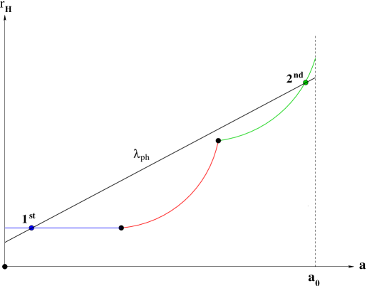
Figure 1: The first and second horizon crossings of the physical wavelength $\lambda_{\rm ph}$. The                      Hubble radius $r_{H}$ is constant during inflation (blue), behaves like $r_{H}\,\sim\,a^{2}$ during radiation (red), and like $r_{H}\,\sim\,a^{\frac{3}{2}}$ during matter domination (green). The present is at $a_{0}$. The graph is not properly scaled.

We can be more precise by defining the dimensionless variable $x$ which represents the physical wave number in Hubble units:

$$x(t,k)\;\equiv\;\frac{k}{a(t)\,H(t)}\;\;,$$ (9)

and in terms of which horizon crossing means:

$$Horizon\;Crossing\quad\Longrightarrow\quad x(t,k)\;=\;1\;\;.$$ (10)

When the deceleration parameter $q$ is constant, which is a good approximation during the dominant phases in the history of the universe, the following relation is valid:

$$q(t)\;=\;{\bar{q}}\quad\Longrightarrow\quad x(t,k)\;=\;x(t_{i},k)\,\left(\,\frac{1+z(t_{i})}{1+z(t)}\,\right)^{\bar{q}}\;\;.$$ (11)

If we take the initial time instant $t_{i}$ to signify the onset of inflation, it becomes apparent that during inflation $x$ decreases with time: ${\bar{q}}$ is negative in this era while $z$ is an ever decreasing function of time. Thus, the modes of interest start with $x$ larger than 1 and achieve condition (10) – first horizon crossing – as the universe still inflates. After first horizon crossing, the variable $x$ for these modes further decreases and becomes very much less than 1. However, post-inflationary evolution is characterized by positive ${\bar{q}}$ and, hence, $x$ increases during this era. The modes of physical interest are such that condition (10) is satisfied again – second horizon crossing – before the present.

Moreover, we note that significant fluctuations do not occur for all fields, only for those which are both much lighter than the inflationary Hubble parameter and also not conformally invariant. These two requirements mean we need consider only gravitons and light, minimally coupled scalars.

It is unnecessary to discuss invariant characterizations of cosmological perturbations. The fully general and invariant formula of Sachs and Wolfe – which is reviewed in Section 2 – allows us to solve for the perturbations with any convenient choice of gauge and field variables. Although we shall not work beyond linearized order, it is worth noting that the result of Sachs and Wolfe can be extended to any desired order in the weak field expansion. The method is applied for the generic system of a graviton with a massless, minimally coupled scalar in Section 3. The scalar and tensor power spectra are derived in Sections 4 and 5 respectively. In both cases improved estimates are obtained. Our conclusions comprise Section 6. The basics of the evolution dependent improvement factors have been summarized in the Appendix. Another Appendix describes a model in which the slow roll paradigm completely breaks down but our methods can still be employed.

2 The Sachs and Wolfe Effect

The gravitational field equations are:

$$G_{\mu\nu}\equiv R_{\mu\nu}-\frac{1}{2}g_{\mu\nu}R=8\pi G\;T_{\mu\nu}\;\;,$$ (12)

in which $G$ is the Newton constant. A spatially homogeneous and isotropic universe can be conveniently represented by the stress tensor $T_{\mu\nu}$ of a perfect fluid with energy density $\rho$, pressure $p$ and 4-velocity $u^{\mu}$:

$$T_{\mu\nu}\;=\;(\rho+p)\,u_{\mu}\,u_{\nu}\;+\;p\,g_{\mu\nu}\;\;,$$ (13)

where $u^{\mu}$ obeys:

$$u^{\mu}\,u^{\nu}\,g_{\mu\nu}\;=\;-1\;\;.$$ (14)

To account for the observed structures and obtain a more realistic cosmological description, deviations from homogeneity and isotropy are essential. Without any reference to their origin, it is simple to incorporate such departures as linear perturbations on the dynamical variables of the system:

$$g_{\mu\nu}(\eta,{\vec{x}}) = {\bar{g}}_{\mu\nu}(\eta)\;+\;\delta g_{\mu\nu}(\eta,{\vec{x}})\;\;,$$ (15)

$$\rho(\eta,{\vec{x}}) = {\bar{\rho}}(\eta)\;+\;\delta\rho(\eta,{\vec{x}})\;\;,$$ (16)

$$p(\eta,{\vec{x}}) = {\bar{p}}(\eta)\;+\;\delta p(\eta,{\vec{x}})\;\;.$$ (17)

The unperturbed metric field ${\bar{g}}_{\mu\nu}$ belongs to the Robertson-Walker class of spacetimes and is, therefore, conformally flat and characterized by scale factor $a$:

$${\bar{g}}_{\mu\nu}\;=\;a^{2}(\eta)\,\eta_{\mu\nu}\;\;.$$ (18)

The unperturbed ${\bar{\rho}}$ and ${\bar{p}}$ correspond to the average energy density and pressure of the physical system respectively. The arbitrariness in the choice of coordinates is resolved by employing a frame that moves with the fluid:

$$g_{00}(\eta,{\vec{x}}) = -1\;\;,$$ (19)

$$G^{\,i}_{\;\,0}(\eta,{\vec{x}}) = 0\;\;\Longleftrightarrow\;\;u^{\mu}(\eta,{\vec{x}})\;=\;a^{-1}(\eta)\;\delta^{\mu}_{\;\;0}\;\;.$$ (20)

It is important to note the relation between co-moving and conformal time intervals:

$$dt\;=\;a(\eta)\;d\eta\;\;.$$ (21)

Figure 2: The light emission $(\eta_{E}\,,\,{\vec{x}})$ and reception $(\eta_{R}\,,\,{\vec{0}})$ events, and the lightlike                       geodesic $\chi^{\mu}$.

Sachs and Wolfe have computed [20] the redshift accumulated by a light ray as it travels in the presence of (15) from its emission to its reception (see Figure 2). The result is quite general as the only relevant ingredient is the metric field perturbation:

$$\delta g_{\mu\nu}\;\equiv\;a^{2}(\eta)\;h_{\mu\nu}(\eta,{\vec{x}})\;\;.$$ (22)

If the light signal is observed from direction ${\widehat{e}}$, the wavelength shift $z({\widehat{e}})$ is given by:

$$1\,+\,z({\widehat{e}})\;=\;\frac{\left[\,u^{\mu}\,k_{\mu}\,\right]_{E}}{\left[\,u^{\mu}\,k_{\mu}\,\right]_{R}}\;\;,$$ (23)

where $E$ and $R$ stand for the emission and reception events respectively, and where $k^{\mu}$ is the 4-momentum of the light ray:

$$k^{\mu}(\tau)\;=\;{\dot{\chi}}^{\mu}(\tau)\;\;.$$ (24)

The lightlike geodesic ${\chi}^{\mu}$ satisfies:

$${\ddot{\chi}}^{\mu}(\tau)\,+\,\Gamma^{\mu}_{\;\;\alpha\beta}[\chi(\tau)]\;{\dot{\chi}}^{\alpha}(\tau)\;{\dot{\chi}}^{\beta}(\tau) = 0\;\;,$$ (25)

$$g_{\alpha\beta}[\chi(\tau)]\;{\dot{\chi}}^{\alpha}(\tau)\;{\dot{\chi}}^{\beta}(\tau) = 0\;\;,$$ (26)

and (25-26) can be integrated to give the following result for $z({\widehat{e}})$ to first order in the perturbation $h_{\mu\nu}$ [20]:

$$1\,+\,z({\widehat{e}}) = \frac{a(\eta_{R})}{a(\eta_{E})}\,\times$$

$$\left\{\,1\,-\,\int_{0}^{\eta_{R}-\eta_{E}}d\sigma\left[\,{\widehat{e}}^{\,i}\;h_{0i\,,\,0}(x)\,-\,\frac{1}{2}\,{\widehat{e}}^{\,i}\,{\widehat{e}}^{\,j}\;h_{ij\,,\,0}(x)\,\right]_{x^{\mu}\,=\,(\,\eta_{R}-\sigma,\,\sigma{\widehat{e}}\,)}\,\right\}\,.$$

Suppose that thermal radiation of average temperature $T_{E}$ was emitted from a spacelike surface at the time $\eta_{E}$ of the coordinate system. Then, at the reception event $(\eta_{R},{\vec{0}})$:

$$T_{R}({\widehat{e}})\;=\;\frac{T_{E}({\widehat{e}})}{1+z({\widehat{e}})}\;\;,$$ (28)

so that the first order temperature fluctuation observed from direction ${\widehat{e}}$ is:

$$\frac{\Delta T_{R}}{T_{R}}({\widehat{e}}) = \frac{\Delta T_{E}}{T_{E}}({\widehat{e}})\,+$$

$$\int_{t_{E}}^{t_{R}}dt\;\left[\,{\widehat{e}}^{\,i}\;h_{0i\,,\,t\,}(x)\,-\,\frac{1}{2}\,{\widehat{e}}^{\,i}\,{\widehat{e}}^{\,j}\;h_{ij\,,\,t\,}(x)\,\right]_{x^{\mu}\,=\,\left(\,t\,,\;{\widehat{e}}\int_{t}^{t_{R}}\,dt^{\prime}\;a^{-1}(t^{\prime})\,\right)}\;\;,$$

and has been expressed in terms of the co-moving time $t$. Since the accumulated wavelength shift and the temperature fluctuation are observables, expressions (2) and (2) are manifestly gauge invariant.

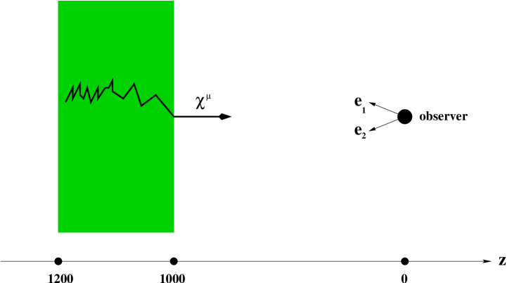
Figure 3: A typical lightlike geodesic $\chi^{\mu}$ on its way to the observer. The graph is not                      properly scaled.

The Cosmic Microwave Background Radiation (CMBR) consists of photons emitted during the period of decoupling. What is measured is the product of temperature fluctuations simultaneously observed from two different directions (see Figure 3). Thus, the connection between the measured quantity and the quantum mechanical origin of these fluctuations comes from the study of:

$$\left\langle\Omega\left|\;\frac{\Delta T_{R}}{T_{R}}({\widehat{e}_{1}})\;\;\frac{\Delta T_{R}}{T_{R}}({\widehat{e}_{2}})\;\right|\Omega\right\rangle\;\;,$$ (30)

for the appropriate vacuum state $|\Omega\rangle$.

3 The Perturbations of the Graviton-Scalar System

The Lagrangian describing the system of the graviton and a minimally coupled scalar is:

$${\cal L}\;=\;{1\over 16\pi G}\,R\,\sqrt{-g}\;-\;\frac{1}{2}\,\partial_{\mu}\varphi\;\partial_{\nu}\varphi\;g^{\mu\nu}\sqrt{-g}\;-\;V(\varphi)\,\sqrt{-g}\;\;.$$ (31)

Its dynamical variables are the metric field $g_{\mu\nu}$ and the scalar $\varphi$. Both are expressed as a background plus a quantum field:

$$g_{\mu\nu}(\eta,{\vec{x}}) = a^{2}(\eta)\,\Bigl{(}\,\eta_{\mu\nu}\;+\;h_{\mu\nu}(\eta,{\vec{x}})\,\Bigr{)}\;\;,$$ (32)

$$\equiv a^{2}(\eta)\,\Bigl{(}\,\eta_{\mu\nu}\;+\;\kappa\,\psi_{\mu\nu}(\eta,{\vec{x}})\,\Bigr{)}\;\;,$$ (33)

$$\varphi(\eta,{\vec{x}}) = \varphi_{0}(\eta)\;+\;\phi(\eta,{\vec{x}})\;\;,$$ (34)

where $\kappa^{2}\equiv 16\pi G$ is the loop counting parameter of quantum gravity.

The background Einstein equations are:

$$3H^{2} = 8\pi G\,\Bigl{(}\,\frac{1}{2}\,\dot{\varphi}_{0}^{2}+V(\varphi_{0})\,\Bigr{)}\;\;,$$ (35)

$$(-1+2q)H^{2} = 8\pi G\,\Bigl{(}\,\frac{1}{2}\,\dot{\varphi}_{0}^{2}-V(\varphi_{0})\,\Bigr{)}\;\;,$$ (36)

where an overdot represents differentiation with respect to the co-moving time $t$. Although it is traditional to regard the potential as known and then infer the scale factor, with our method it is more convenient to regard $a(t)$ – and hence $H(t)=\dot{a}/a$ and $q(t)=-a\ddot{a}/\dot{a}^{2}$ – as a known function from which the background scalar and the potential can be expressed as follows:

$$\dot{\varphi}_{0} = -\sqrt{1+q(t)}\;\;\frac{H(t)}{\sqrt{4\pi G}}\;\;,$$ (37)

$$V(\varphi_{0}) = \Bigl{(}2-q(t)\Bigr{)}\;\frac{H^{2}(t)}{8\pi G}\;\;.$$ (38)

We parameterize the third derivative of $a(t)$ using the variable:

$$r(t)\;\equiv\;\frac{1}{H(t)}\;\frac{d}{dt}\ln\Bigl{(}\sqrt{1+q(t)}\,\Bigr{)}\;\;.$$ (39)

Hence, the derivative of the potential is:

$$V^{\prime}(\varphi_{0})\;=\;\Bigl{(}\,2-q(t)+r(t)\,\Bigr{)}\;\sqrt{1+q(t)}\;\frac{H^{2}(t)}{\sqrt{4\pi G}}\;\;.$$ (40)

Higher derivatives of the potential can obviously be obtained by taking higher time derivatives of the scale factor, for example:

$$V^{\prime\prime}(\varphi_{0})\;=\;\Bigg{(}\,3q(t)\,r(t)-r^{2}(t)-\frac{\dot{r}(t)}{H(t)}\,\Bigg{)}\;H^{2}(t)\;\;.$$ (41)

A convenient diagonalization of the linearized system is given in [21, 22] and is summarized in [11]. By employing a generalized de Donder gauge condition:

$$F_{\mu}\;\equiv\;a\left[\,\psi^{\nu}_{~{}\mu\,,\,\nu}\,-\,\frac{1}{2}\,\psi^{\nu}_{~{}\nu\,,\,\mu}\,-\,2\,aH\,\psi_{\mu 0}\,+\,2\delta^{0}_{~{}\mu}\,{\sqrt{1+q}}\;aH\,\phi\,\right]\;=\;0\;\;,$$ (42)

all linearized fields can be expressed in terms of:

$$\psi^{TT}_{ij}(\eta,{\vec{x}}) = \int\frac{d^{3}k}{(2\pi)^{3}}\;\sum_{s}\left\{\,\epsilon_{ij}({\vec{k}},s)\;U_{A}(\eta,k)\;e^{i{\vec{k}}\cdot{\vec{x}}}\;\alpha({\vec{k}},s)\;+\;(c.c.)\,\right\}\;,\qquad$$ (43)

$$\psi_{00}(\eta,{\vec{x}}) = \int\frac{d^{3}k}{(2\pi)^{3}}\;\left\{\,U_{C}(\eta,k)\;e^{i{\vec{k}}\cdot{\vec{x}}}\;Y({\vec{k}})\;+\;(c.c.)\,\right\}\;,$$ (44)

as follows:

$$\psi_{0i}(\eta,{\vec{x}}) = 0\;\;,$$ (45)

$$\psi_{ij}(\eta,{\vec{x}}) = \delta_{ij}\;\psi_{00}(\eta,{\vec{x}})\;+\;\psi^{TT}_{ij}(\eta,{\vec{x}})\;\;,$$ (46)

$$\phi(\eta,{\vec{x}}) = \frac{1}{\sqrt{1+q(t)}}\;\;\frac{1}{H(t)\,a(t)}\;\;\frac{\partial}{\partial t}\Bigl{(}\,a(t)\;\psi_{00}(\eta,{\vec{x}})\,\Bigr{)}\;\;,$$ (47)

The mode functions $U_{A,C}$ are of the form:

$$U_{A}(\eta,k) \equiv \frac{\sqrt{2}}{a(t)}\;Q_{A}(\eta,k)\;\;,$$ (48)

$$U_{C}(\eta,k) \equiv -\,\sqrt{1+q(t)}\;H(t)\;\frac{1}{k}\,Q_{C}(\eta,k)\;\;,$$ (49)

where $Q_{A,C}$ obey [11]:

$$Q^{{}^{\prime\prime}}_{A,C}\;+\;\left[\,k^{2}\,-\,\frac{\theta^{{}^{\prime\prime}}_{A,C}}{\theta_{A,C}}\,\right]\,Q_{A,C}=0\;\;,$$ (50)

$$\theta_{A}\;\equiv\;a\quad,\quad\theta_{C}\;\equiv\;\frac{1}{a\,\sqrt{1+q}}\;\;.$$ (51)

The graviton and scalar creation and annihilation operators are canonically normalized:

$$\left[\,\alpha({\vec{k}},s)\;,\;\alpha^{\dagger}({\vec{k}}^{\prime},s^{\prime})\,\right] = (2\pi)^{3}\;\delta^{3}({\vec{k}}\,-\,{\vec{k}}^{\prime})\;\delta_{ss^{\prime}}\;\;,$$ (52)

$$\left[\,Y({\vec{k}})\;,\;Y^{\dagger}({\vec{k}}^{\prime})\,\right] = (2\pi)^{3}\;\delta^{3}({\vec{k}}\,-\,{\vec{k}}^{\prime})\;\;.$$ (53)

The graviton polarization tensor is purely spatial, transverse and traceless:

$$\epsilon_{0\mu}({\vec{k}},s)\;=\;k_{i}\,\epsilon_{ij}({\vec{k}},s)\;=\;\epsilon_{ii}({\vec{k}},s)\;=\;0\;\;.$$ (54)

Moreover, summing products of two polarization tensors gives:

$$\sum_{s}\epsilon_{ij}({\vec{k}},s)\;\epsilon^{*}_{mn}(\vec{k},s) = \frac{1}{2}\;\Bigl{[}\,\Pi_{im}\,\Pi_{jn}\,+\,\Pi_{in}\,\Pi_{jm}\,-\,\Pi_{ij}\,\Pi_{mn}\,\Bigr{]}\;\;,$$ (55)

$$\Pi_{ij} \equiv \delta_{ij}\,-\,\widehat{k}_{i}\,\widehat{k}_{j}\;\;,$$ (56)

where $\Pi_{ij}$ is the transverse projector.

In order to apply the basic formula (2) for the first order temperature fluctuation, we must transform the linearized fields (44-47) from obeying the gauge condition (42) to satisfying the co-moving gauge conditions (19-20). This is achieved by effecting the field-dependent coordinate transformation:

$$x^{\mu}(x^{\prime})\;\equiv\;x^{\prime\,\mu}\,+\,\kappa\;\varepsilon^{\mu}(x^{\prime})\;\;,$$ (57)

which imposes the co-moving gauge conditions:

$$\varepsilon_{0}(\eta,{\vec{x}}) = -\,\frac{1}{2a(\eta)}\,\int_{\eta_{E}}^{\eta}d\eta^{\prime}\;a(\eta^{\prime})\;\psi_{00}(\eta^{\prime},{\vec{x}})\;\;,$$ (58)

$$\varepsilon_{i}(\eta,{\vec{x}}) = \int_{\eta_{E}}^{\eta}d\eta^{\prime}\,\left[\,\psi_{0i}(\eta^{\prime},{\vec{x}})\,+\,\frac{\phi_{,\,i\,}(\eta^{\prime},{\vec{x}})}{\kappa\,\varphi_{0}^{\prime}(\eta^{\prime})}\,\right]\;\;,$$ (59)

on the linearized fields. In particular, since under any infinitesimal coordinate transformation (57) the graviton field transforms to:

$${\widetilde{\psi}_{\mu\nu}}\;=\;\psi_{\mu\nu}\,+\,2\,\varepsilon_{(\mu\,,\,\nu)}\,-\,2Ha\,\varepsilon_{0}\,\eta_{\mu\nu}\;\;,$$ (60)

for the specific choice (58-59) we obtain:

$${\widetilde{\psi}_{00}}(\eta,{\vec{x}}) = 0\;\;,$$ (61)

$${\widetilde{\psi}_{0i}}(\eta,{\vec{x}}) = -\,\frac{1}{2a(\eta)}\,\int_{\eta_{E}}^{\eta}d\eta^{\prime}\;a(\eta^{\prime})\;\psi_{00\,,\,i}(\eta^{\prime},{\vec{x}})\,-\,\frac{\phi_{,\,i\,}(\eta,{\vec{x}})}{\kappa\,\varphi_{0}^{\prime}(\eta)}\;\;,$$ (62)

$${\widetilde{\psi}_{ij}}(\eta,{\vec{x}}) = \psi^{TT}_{ij}(\eta,{\vec{x}})\,+\,\delta_{ij}\left[\,\psi_{00}(\eta,{\vec{x}})\,+\,H(\eta)\int_{\eta_{E}}^{\eta}d\eta^{\prime}\;a(\eta^{\prime})\;\psi_{00}(\eta^{\prime},{\vec{x}})\,\right]\quad$$ (63)

$$-\,2\int_{\eta_{E}}^{\eta}d\eta^{\prime}\;\frac{\phi_{,\,ij\,}(\eta^{\prime},{\vec{x}})}{\kappa\,\varphi_{0}^{\prime}(\eta^{\prime})}\;\;.$$

Thus, by construction the graviton field (61-63) obeys (19-20). Keeping in mind the definition (33), the first order temperature fluctuation (2) becomes:

$$\frac{\Delta T_{R}}{T_{R}}({\widehat{e}}) = \frac{\Delta T_{E}}{T_{E}}({\widehat{e}})\,+$$

$$\kappa\int_{\eta_{E}}^{\eta_{R}}d\eta^{\prime}\;\left[\,{\widehat{e}}^{\,i}\;{\widetilde{\psi}}_{0i\,,\,0}(x)\,-\,\frac{1}{2}\,{\widehat{e}}^{\,i}\,{\widehat{e}}^{\,j}\;{\widetilde{\psi}}_{ij\,,\,0}(x)\,\right]_{x^{\mu}\,=\,\left(\,\eta^{\prime}\,,\;(\eta_{R}\,-\,\eta^{\prime})\;{\widehat{e}}\;\right)}\;\;.$$

Further reduction of (3) uses:

$${\widehat{e}}^{\,i}\;{\widetilde{\psi}}_{0i\,,\,0}(\eta,{\vec{x}}) = {\widehat{e}}^{\,i}\,\Biggl{[}\,-\frac{1}{2}\,\psi_{00\,,\,i}(\eta,{\vec{x}})\,+\,\frac{H(\eta)}{2}\int_{\eta_{E}}^{\eta}d\eta^{\prime}\;a(\eta^{\prime})\;\psi_{00\,,\,i}(\eta^{\prime},{\vec{x}})$$ (65)

$$\hskip 19.91684pt-\,\left(\,\frac{\phi(\eta,{\vec{x}})}{\kappa\,{\varphi_{0}}^{\prime}(\eta)}\,\right)_{,\,0i}\;\Biggr{]}\;\;,$$

together with:

$$-\,\frac{1}{2}\,{\widehat{e}}^{\,i}\,{\widehat{e}}^{\,j}\;{\widetilde{\psi}}_{ij\,,\,0}(\eta,{\vec{x}}) = {\widehat{e}}^{\,i}\,{\widehat{e}}^{\,j}\,\left[\,-\,\frac{1}{2}\,\psi^{TT}_{ij\,,\,0}(\eta,{\vec{x}})\,+\,\left(\,\frac{\phi(\eta,{\vec{x}})}{\kappa\,{\varphi_{0}}^{\prime}(\eta)}\,\right)_{,\,ij}\;\right]$$ (66)

$$\hskip 36.98866pt-\,\frac{1}{2}\Biggl{[}\,\psi_{00\,,\,0}(\eta,{\vec{x}})\,+\,\frac{a^{\prime}(\eta)}{a(\eta)}\;\psi_{00}(\eta,{\vec{x}})$$

$$\hskip 62.59596pt+\,H^{\prime}(\eta)\int_{\eta_{E}}^{\eta}d\eta^{\prime}\;a(\eta^{\prime})\;\psi_{00}(\eta^{\prime},{\vec{x}})\,\Biggr{]}\;.$$

A straightforward computation leads to the final form for the first order temperature fluctuations:

$$\frac{\Delta T_{R}}{T_{R}}({\widehat{e}}) = \frac{\Delta T_{E}}{T_{E}}({\widehat{e}})\;+$$

$$\frac{\kappa}{2}\left[\,\psi_{00}(\eta_{R},{\vec{0}}\hskip 1.42271pt)\,-\,H_{R}\int_{\eta_{E}}^{\eta_{R}}d\eta^{\prime}\;a(\eta^{\prime})\;\psi_{00}(\eta^{\prime},{\vec{0}}\hskip 1.42271pt)\,\right]$$

$$-\;\frac{{\widehat{e}}^{\,i}\;\phi_{,\,i\,}(\eta_{R},{\vec{0}}\hskip 1.42271pt)}{{\varphi_{0}}^{\prime}(\eta_{R})}\;+\;\frac{{\widehat{e}}^{\,i}\;\phi_{,\,i\,}(\,\eta_{E}\,,\,(\eta_{R}-\eta_{E})\,{\widehat{e}}\,)}{{\varphi_{0}}^{\prime}(\eta_{R})}$$

$$-\;\frac{\kappa}{2}\;\psi_{00}(\,\eta_{E}\,,\,(\eta_{R}-\eta_{E})\,{\widehat{e}}\,)\;-\;\kappa\int_{\eta_{E}}^{\eta_{R}}d\eta^{\prime}\;\psi_{00\,,\,0}(\,\eta^{\prime}\,,\,(\eta_{R}-\eta^{\prime})\,{\widehat{e}}\,)$$

$$-\;\frac{\kappa}{2}\;{\widehat{e}}^{\,i}\,{\widehat{e}}^{\,j}\int_{\eta_{E}}^{\eta_{R}}d\eta^{\prime}\;\psi^{TT}_{ij\,,\,0}(\,\eta^{\prime}\,,\,(\eta_{R}-\eta^{\prime})\,{\widehat{e}}\,)\;\;.$$

The right hand side of (3) consists of a part associated with the temperature fluctuations of the emitting surface plus seven terms. The first two of the latter have no angular dependence and belong to the monopole contribution. The third term is the dipole contribution while the fourth is the Sachs-Wolfe velocity potential term. The spectra of scalar and tensor perturbations that are usually reported reside in the fifth (the Sachs-Wolfe potential term) and seventh terms respectively. The remaining sixth term is sometimes called the integrated Sachs-Wolfe effect.

4 The Tensor Power Spectrum

In 1979, Starobinskiĭ [23] became the first to calculate the tensor power spectrum from what would later be called a model of inflation. Subsequent computations were in 1982 made by Rubakov, Sazhim and Veryaskin [24] and by Fabbri and Pollock [25]. The definitive result was obtained by Starobinskiĭ in 1985 [26]. These calculations all depend upon a normalization for the late-time mode functions whose precise determination is our only improvement. However, we shall also carry out the computation in a slightly different fashion.

The part of (3) relevant to tensor perturbations is:

$$\frac{\Delta T_{R}}{T_{R}}({\widehat{e}})\,\Big{|}_{\,h}\;=\;-\,\frac{\kappa}{2}\;{\widehat{e}}^{\,i}\,{\widehat{e}}^{\,j}\int_{\eta_{E}}^{\eta_{R}}d\eta^{\prime}\;\psi^{TT}_{ij\,,\,0}(\,\eta^{\prime}\,,\,(\eta_{R}-\eta^{\prime})\,{\widehat{e}}\,)\;\;,$$ (68)

and can be expressed as a sum over graviton momenta and polarizations:

$$\frac{\Delta T_{R}}{T_{R}}({\widehat{e}})\,\Big{|}_{\,h}\;=\;\int\frac{d^{3}k}{(2\pi)^{3}}\;\sum_{s}\left\{\,h({\widehat{e}},{\vec{k}})\;\;{\widehat{e}}^{\,i}\,{\widehat{e}}^{\,j}\,\epsilon_{ij}(\vec{k},s)\;\,\alpha(\vec{k},s)\;+\;(c.c.)\,\right\}\;,$$ (69)

where the scalar response function is:

$$h({\widehat{e}},{\vec{k}})\;=\;-\frac{\kappa}{2}\,\int_{t_{E}}^{t_{R}}dt\;\left(\,\frac{\partial}{\partial t}\;U_{A}(t,k)\,\right)\;\exp\left[\,i{\vec{k}}\cdot{\widehat{e}}\int_{t}^{t_{R}}dt^{\prime}\;a^{-1}(t^{\prime})\,\right]\;\;.$$ (70)

It is straightforward to compute the expectation value (30) in the presence of the state which was empty of gravitons in the distant past:

$$\alpha({\vec{k}},s)\,|\Omega\rangle\;=\;0\;\;,$$ (71)

and obtain:

$$\left\langle\Omega\left|\;\frac{\Delta T_{R}}{T_{R}}({\widehat{e}_{1}})\;\;\frac{\Delta T_{R}}{T_{R}}({\widehat{e}_{2}})\;\right|\Omega\right\rangle_{h} = \int\frac{d^{3}k}{(2\pi)^{3}}\;\;h({\widehat{e}}_{1},{\vec{k}})\;\;h^{*}({\widehat{e}}_{2},{\vec{k}})$$

$$\hskip 5.69046pt\times\;{\widehat{e}}^{\,i}_{1}\,{\widehat{e}}^{\,j}_{1}\,{\widehat{e}}^{\,m}_{2}\,{\widehat{e}}^{\,n}_{2}\,\left[\,\Pi_{im}\,\Pi_{jn}\,-\,\frac{1}{2}\Pi_{ij}\,\Pi_{mn}\,\right]\;.$$

The scalar response function (70) can be explicitly evaluated because the physical process occurs entirely during the epoch of matter domination. If we assume that the onset of matter domination occurred at a time $t_{M}$, when the Hubble parameter and scale factor were $H_{M}$ and $a_{M}$ respectively, then at later times:

$$Matter\quad\Longrightarrow\quad H(t) = \frac{H_{M}}{1\,+\,\frac{3}{2}H_{M}\,(t-t_{M})}\;\;,$$ (73)

$$a(t) = a_{M}\left[\,1\,+\,\frac{3}{2}H_{M}\,(t-t_{M})\,\right]^{\frac{2}{3}}\;\;.$$ (74)

In view of (73-74), the dimensionless variable (9) equals:

$$Matter\quad\Longrightarrow\quad x(t,k)\;=\;x(t_{M},k)\,\left[\,1\,+\,\frac{3}{2}H_{M}\,(t-t_{M})\,\right]^{\frac{1}{3}}\;\;,$$ (75)

In terms of $x$, the radial component of a lightlike geodesic times $k$ takes the form:

$$Matter\quad\Longrightarrow\quad k\,\int_{t}^{t_{R}}\;\frac{dt^{\prime}}{a(t^{\prime})}\;=\;2x(t_{R},k)\,-\,2x(t,k)\;\;,$$ (76)

and the scalar response function (70) becomes:

$$h(\widehat{e},{\vec{k}})\;=\;-\frac{\kappa}{2}\;\int_{x_{E}}^{x_{R}}\;dx\;\left(\,\frac{\partial}{\partial x}\;U_{A}(t,k)\,\right)\;e^{2i\,{\widehat{k}}\,\cdot\,{\widehat{e}}\,(x_{R}-x)}\;\;.$$ (77)

Further progress in the evaluation of the scalar response function (77) requires an explicit form for the mode function. Indeed, the source of our improved estimate for the graviton power spectrum is our improved derivation of the graviton mode functions [10]. Since the physical process under study involves modes that underwent first horizon crossing at $t=t_{1}$, the relevant form of the mode functions for $t>t_{1}$ is [11]:

$$U_{A}(t,k)\;=\;\frac{-iH_{1}}{\sqrt{k^{3}}}\;\frac{\Gamma(1-\nu)\;J_{-\nu}(-\frac{x}{q})}{(-\frac{x}{2q})^{-\nu}}\;\times\;{\cal C}_{1A}(k)\,\times\,{\cal C}_{iA}(k)\;\;.$$ (78)

It consists of three factors, the first of which is the time dependent part:

$$\frac{\Gamma(1-\nu)\;J_{-\nu}(-\frac{x}{q})}{(-\frac{x}{2q})^{-\nu}}\Bigg{|}_{\,q\,=\,\frac{1}{2}\,,\;\nu\,=\,-\frac{3}{2}}=\;3\,\sqrt{\frac{\pi}{2}}\;\frac{J_{\frac{3}{2}}(2x)}{(2x)^{\frac{3}{2}}}\;\;.$$ (79)

This is a standard result. The remaining two factors in (78) represent our improvement to the normalization of the mode functions; ${\cal C}_{1A}$ depends upon the state of the system at first horizon crossing:

$${\cal C}_{1A}(k)\;\equiv\;\frac{\frac{1}{\sqrt{\pi}}\;\Gamma(\,\frac{1}{2}-\frac{1}{q_{1}}\,)}{(-\frac{1}{2q_{1}})^{-\frac{1}{q_{1}}}}\;\;.$$ (80)

To get a feeling for ${\cal C}_{1A}$, it is important to note that for perfect de Sitter inflation it equals one:

$$q_{1}\,=\,-1\quad\Longrightarrow\quad{\cal C}_{1A}(k)\,=\,1\;\;,$$ (81)

while for a more realistic situation one finds to first order:

$$q_{1}(k) = -1\,+\,\Delta q(k)\quad\Longrightarrow\quad$$

$${\cal C}_{1A}(k) = 1\,+\,\Bigl{[}\,\psi({\scriptstyle\frac{3}{2}})\,+\,\ln 2\,-\,1\,\Bigr{]}\Delta q(k)\quad,\quad\psi(z)\equiv\frac{\Gamma^{\prime}(z)}{\Gamma(z)}\;\;.\qquad$$ (82)

The factor ${\cal C}_{iA}$ depends upon previous evolution. Had there been no evolution in $q$ from the initial time $t_{i}$ to $t_{1}$, its value would be one:

$$q(t)\,=\,{\bar{q}}\quad\Longrightarrow\quad{\cal C}_{iA}(k)=1\;\;.$$ (83)

When – as is the physical case – there is a mild evolution, it results in small deviations about (83) whose explicit form is given in the first Appendix.

In view of (79), we can express (78) with its conventional slow-roll normalization times the two correction factors:

$$U_{A}(t,k)\;=\;\frac{-iH_{1}}{\sqrt{k^{3}}}\;3\left[\,\frac{\sin(2x)}{8x^{3}}\,-\,\frac{\cos(2x)}{4x^{2}}\,\right]\,\times\,{\cal C}_{1A}(k)\,\times\,{\cal C}_{iA}(k)\;\;.$$ (84)

With the infrared approximation (84) it is possible to exactly evaluate the scalar response function (77):

$$h(\widehat{e},{\vec{k}}) = \frac{i\kappa H_{1}}{\sqrt{2k^{3}}}\;\frac{3}{\sqrt{2}}\;{\cal C}_{1A}\;{\cal C}_{iA}\;e^{2i\,w\,x_{R}}\;\Biggl{\{}\,\Biggl{[}\,\frac{\sin(2x)}{8x^{3}}\,-\,\frac{\cos(2x)}{4x^{2}}$$

$$-\,iw\left(\,\frac{\sin(2x)}{8x^{2}}\,-\,\frac{\cos(2x)}{4x}\,\right)\,-\,w^{2}\;\frac{\sin(2x)}{4x}\;\Biggr{]}e^{-2i\,wx}$$

$$+\,\frac{w}{4}\,(1-w^{2})\Bigl{[}\,{\rm Ei}\Bigl{(}\,2i(1-w)x\,\Bigr{)}\,-\,{\rm Ei}\Bigl{(}\,-2i(1+w)x\,\Bigr{)}\,\Bigr{]}\,\Biggr{\}}\,\Biggr{|}_{x_{E}}^{x_{R}}\;\;,$$

where, to economize on writing, we have defined $w\equiv\widehat{k}\cdot\widehat{e}$ as the cosine of the angle between the unit vectors $\widehat{k}$ and $\widehat{e}$. However, there is no point in retaining the full complexity of this result. It is easy to check that the term inside the curly brackets falls like $x^{-2}$ for large $x$. Therefore, potentially observable effects must derive from modes which had not yet experienced second horizon crossing at the time of emission. This implies $x_{E}\ll 1$. The modes which produce anisotropies within our current horizon volume must also have experienced second horizon crossing by the time of reception. Hence we can also assume $x_{R}\gg 1$. It follows that the only significant contribution comes from the lower limit, for which we may as well take the limiting form relevant to small $x_{E}$:

$$h(\widehat{e},{\vec{k}})\,\Bigg{|}_{\,x_{E}\,\ll\,1}^{\,x_{R}\,\gg\,1} = -\frac{i\kappa H_{1}}{\sqrt{k^{3}}}\;{\cal C}_{1A}\;{\cal C}_{iA}\;e^{2i\,w\,x_{R}}$$

$$\times\,\left\{\,\frac{1}{2}\,-\,\frac{3}{4}w^{2}\,-\,\frac{3}{8}\,w\,(1-w^{2})\left[\,\ln\left(\frac{1+w}{1-w}\right)\,+\,i\pi\,\right]\,\right\}\;\;.$$

The angular dependence in our expression (4) for the scalar response function is complicated. However, one can recognize some of the factors as spherical harmonics with zenith angle $\theta={\rm arccos}(\widehat{e}\cdot\widehat{k})$ and azimuthal angle $\phi=0\,$:

$$\frac{1}{2}\,-\,\frac{3}{4}\,w^{2} = \frac{\sqrt{\pi}}{2}\,Y_{00}\,-\,\sqrt{\frac{\pi}{5}}\,Y_{20}\;\;,$$ (87)

$$-\frac{3}{8}\,w\,(1-w^{2}) = -\frac{3}{2}\,\sqrt{\frac{2\pi}{105}}\,Y_{32}\;\;.$$ (88)

It makes sense to decompose the scalar response function into a part depending only upon $k\equiv\|\vec{k}\|$ and an angular factor $\Theta$, with the $Y_{00}$ term in the latter bearing unit normalization:

$$h(\widehat{e},{\vec{k}})\,\Bigg{|}_{\,x_{E}\,\ll\,1}^{\,x_{R}\,\gg\,1}\;=\;\frac{-i\kappa H_{1}}{\sqrt{k^{3}}}\;{\cal C}_{1A}\;{\cal C}_{iA}\;\frac{\sqrt{\pi}}{2}\;\Theta(\widehat{e},\vec{k})\;\;.$$ (89)

Obviously:

$$\Theta(\widehat{e},\vec{k})\;\equiv\;\frac{e^{2i\,w\,x_{R}}}{\sqrt{4\pi}}\left\{\,2-3w^{2}-\frac{3}{2}\,w\,(1-w^{2})\left[\,\ln\left(\frac{1+w}{1-w}\right)\,+\,i\pi\,\right]\,\right\}\;\;.$$ (90)

We define the “graviton power spectrum” in terms of the radial factor:

$${\cal P}_{h}(k) \equiv \frac{k^{3}}{4\pi^{2}}\;\Bigl{\|}\,\frac{-i\kappa H_{1}}{\sqrt{k^{3}}}\;{\cal C}_{1A}\;{\cal C}_{iA}\;\frac{\sqrt{\pi}}{2}\,\Bigr{\|}^{2}\;\;,$$ (91)

$$= GH_{1}^{2}(k)\;\;{\cal C}^{2}_{1A}(k)\;\;\|\,{\cal C}_{iA}(k)\,\|^{2}\;\;.$$ (92)

Because the literature abounds with different conventions for this quantity, we correspond ${\cal P}_{h}(k)$ to the symbol $\delta_{h}^{2}(k)$ used by Mukhanov, Feldman and Brandenberger [5], to the variable ${\cal P}_{g}(k)$ used by Liddle and Lyth [6], and to the quantity $A_{T}^{2}(k)$ used by Lidsey et al. [7]:

$${\cal P}_{h}(k)\;=\;\frac{9\pi}{4}\,\delta_{h}^{2}(k)\;=\;\frac{\pi}{16}\,{\cal P}_{g}(k)\;=\;\frac{25\pi}{4}\,A_{T}^{2}(k)\;\;.$$ (93)

Perhaps the clearest specification of ${\cal P}_{h}(k)$ is to state how it enters the temperature correlation function:

$$\left\langle\Omega\left|\;\frac{\Delta T_{R}}{T_{R}}({\widehat{e}_{1}})\;\;\frac{\Delta T_{R}}{T_{R}}({\widehat{e}_{2}})\;\right|\Omega\right\rangle_{h} = 2\int_{0}^{\infty}\frac{dk}{k}\;{\cal P}_{h}(k)\int\frac{d^{2}{\widehat{k}}}{4\pi}\;\Theta({\widehat{e}}_{1},\vec{k})\;\,\Theta^{*}({\widehat{e}}_{2},\vec{k})\;$$ (94)

$$\times\;{\widehat{e}}^{\,i}_{1}\,{\widehat{e}}^{\,j}_{1}\,{\widehat{e}}^{\,m}_{2}\,{\widehat{e}}^{\,n}_{2}\,\left[\,\Pi_{im}\,\Pi_{jn}\,-\,\frac{1}{2}\Pi_{ij}\,\Pi_{mn}\,\right]\;\;.$$

The leading order slow roll result for ${\cal P}_{h}(k)$ is typically expressed in terms of the value of the scalar potential at horizon crossing. Using (38) it can be converted to our notation:

$$\frac{8\pi}{3}G^{2}V_{1}\;=\;GH^{2}_{1}\;\Bigl{(}\,\frac{2-q_{1}}{3}\,\Bigr{)}\;\;.$$ (95)

Our correction factors of $\frac{3}{2-q_{1}}$, $C^{2}_{1A}(k)$ and $\|C_{iA}(k)\|^{2}$ are typically near one for slow roll inflation. Note especially the factor $\|C_{iA}(k)\|^{2}$, which represents the effect of evolution from the beginning of inflation up to horizon crossing, as required by the analysis of Wang, Mukhanov and Steinhardt [13].

It is elementary to verify that there is no monopole contribution to (94) by fixing one of the two directions, for instance ${\widehat{e}}_{2}$, and integrating over the other:

$$Monopole\quad\Longrightarrow\quad\frac{1}{4\pi}\int d^{2}{\widehat{e}}_{1}\;\left\langle\Omega\left|\;\frac{\Delta T_{R}}{T_{R}}({\widehat{e}_{1}})\;\;\frac{\Delta T_{R}}{T_{R}}({\widehat{e}_{2}})\;\right|\Omega\right\rangle_{h}\;\;.$$ (96)

If we take the $z$-axis to be along the ${\widehat{k}}$ direction, we can express ${\widehat{e}_{1}}$ in terms of the zenith angle $\theta$ and azimuthal angle $\phi$:

$${\widehat{e}}_{1}\;=\;(\,\sin\theta\,\cos\phi\;,\;\sin\theta\,\sin\phi\;,\;\cos\theta\,)\;\;.$$ (97)

The resulting azimuthal integration is simple:

$$\int_{0}^{2\pi}\frac{d\phi}{2\pi}\;\;{\widehat{e}}^{\,i}_{1}\,{\widehat{e}}^{\,j}_{1}\;=\;\frac{1}{2}\,\Pi^{ij}\,\sin^{2}\theta\,\;+\;{\widehat{k}}^{\,i}\,{\widehat{k}}^{\,j}\,\cos^{2}\theta\;\;,$$ (98)

and the properties of $\Pi_{ij}$ ensure that (98) gives a vanishing monopole contribution (96).

In a similar fashion, it can be proved that (94) contains no dipole component:

$$Dipole\quad\Longrightarrow\quad\frac{1}{4\pi}\int d^{2}{\widehat{e}}_{1}\;{\widehat{e}}^{\,j}_{1}\;\left\langle\Omega\left|\;\frac{\Delta T_{R}}{T_{R}}({\widehat{e}_{1}})\;\;\frac{\Delta T_{R}}{T_{R}}({\widehat{e}_{2}})\;\right|\Omega\right\rangle_{h}\;=\;0\;\;,$$ (99)

where, as for the monopole case, direction ${\widehat{e}}_{2}$ has been fixed.

5 The Scalar Power Spectrum

The spectrum of scalar perturbations can be computed from the Sachs-Wolfe potential term in (3):

$$\frac{\Delta T_{R}}{T_{R}}({\widehat{e}})\,\Big{|}_{\,{\rm SW}}\;=\;-\;\frac{\kappa}{2}\;\psi_{00}(\,\eta_{E}\,,\,(\eta_{R}-\eta_{E})\,{\widehat{e}}\,)\;\;.$$ (100)

By virtue of (44) we have:

$$\frac{\Delta T_{R}}{T_{R}}({\widehat{e}})\,\Big{|}_{\,{\rm SW}}\;=\;-\,\frac{\kappa}{2}\,\int\frac{d^{3}k}{(2\pi)^{3}}\;\left\{\,U_{C}(\eta_{E},k)\;e^{ik\,(\eta_{R}-\eta_{E})\,{\widehat{k}}\,\cdot\,{\widehat{e}}}\;\;Y({\vec{k}})\;+\;(c.c.)\,\right\}\;\;.$$ (101)

In the presence of the state without any scalars in the distant past:

$$Y({\vec{k}})\,|\Omega\rangle\;=\;0\;\;,$$ (102)

the temperature correlation function (30) becomes:

$$\left\langle\Omega\left|\;\frac{\Delta T_{R}}{T_{R}}({\widehat{e}_{1}})\;\;\frac{\Delta T_{R}}{T_{R}}({\widehat{e}_{2}})\;\right|\Omega\right\rangle_{{\rm SW}} = \frac{\kappa^{2}}{4}\int\frac{d^{3}k}{(2\pi)^{3}}\;\;\|\,U_{C}(\eta_{E},k)\,\|^{2}$$ (103)

$$\hskip 28.45274pt\times\;e^{2i\,(x_{R}-x_{E})\,{\widehat{k}}\,\cdot\,(\,{\widehat{e}}_{1}\,-\,{\widehat{e}}_{2}\,)}\;\;,\qquad\qquad$$

in terms of the dimensionless variable (9).

The relevant form of the mode functions is for $t>t_{1}$ [11]:

$$U_{C}(t,k)\Big{|}_{\,x\,\ll\,1} = \frac{-H_{1}}{\sqrt{2k^{3}\,(1+q_{1})}}\;\frac{H(t)}{a(t)}\;\int_{t_{1}}^{t}dt^{\prime}\;a(t^{\prime})\;[\,1+q(t^{\prime})\,]$$ (104)

$$\hskip 150.79968pt\times\;{\cal C}^{*}_{1C}(k)\,\times\,{\cal C}^{*}_{iC}(k)\;\;,\qquad$$

where $t_{1}$, as always, signals first horizon crossing. In analogy with Section 4, the normalization factor ${\cal C}_{1C}$ depends upon the state of the system at $t_{1}$. It is expressed in terms of $r(t)$ – defined in (39) – and the parameter $q_{C}(t)$:

$$q_{C}(t)\equiv-\,\frac{q(t)}{1+r(t)}\,+\,\frac{\frac{\dot{r}(t)}{H(t)}}{\left[\,1+r(t)\,\right]^{\,2}}\;\;.$$ (105)

The expression is:

$${\cal C}_{1C}\;\equiv\;\frac{\frac{1}{\sqrt{\pi}}\,\Gamma(\,\frac{1}{2}+\frac{1}{q_{1C}}\,)}{\left(\,\frac{1}{2q_{1C}}\,\right)^{\frac{1}{q_{1C}}}}\;e^{-i\frac{\pi}{q_{1C}}}\;\cos({\scriptstyle\frac{\pi}{q_{1C}}})\;(\,1+r_{1}\,)^{\frac{1}{q_{1C}}}\;\;$$ , (106)

$$q_{1C}\;\equiv\;q_{C}(t_{1})\quad,\quad r_{1}\;\equiv\;r(t_{1})\;\;$$ . (107)

During inflation – in fact, quite generally – the parameter $r$ is typically zero. Therefore:

$$r(t)\,=\,0\quad\Longrightarrow\quad q_{C}(t)\,=\,-q(t)\quad\Longrightarrow\quad{\cal C}_{1C}(k)\,=\,{\cal C}_{1A}(k)\;e^{i\frac{\pi}{q_{1}}}\;\cos({\scriptstyle\frac{\pi}{q_{1}}})\qquad$$ (108)

More generally, if $r$ is small we can write to first order:

$$q_{C}(t)\,=\,-q(t)\,+\,q(t)\,r(t)\,+\,\frac{\dot{r}(t)}{H(t)}\;\;.$$ (109)

Consequently, as in (82), we have to first order:

$$q_{1}(k) = -1\,+\,\Delta q(k)\quad\Longrightarrow\quad$$

$$\|\,{\cal C}_{1C}(k)\,\| = 1\,+\,\Bigl{[}\,\psi({\scriptstyle\frac{3}{2}})\,-\,1\,\Bigr{]}\,\left[\,\Delta q(k)\,+\,r_{1}\,-\,\frac{\dot{r}(t)}{H(t)}\,\right]\;\;.$$ (110)

The other factor, ${\cal C}_{iC}$, depends upon evolution from $t_{i}$ to $t_{1}$. Just like ${\cal C}_{iA}$, it equals one when $q$ is constant; its general form can be found in the first Appendix.

Because the physical process takes place entirely during pure matter domination:

$$Matter\quad\Longrightarrow\quad\int_{t_{1}}^{t}dt^{\prime}\;a(t^{\prime})\,[\,1+q(t^{\prime})\,]\;\sim\;\frac{a(t)\,[\,1+q(t)\,]}{H(t)}\;\sim\;\frac{3a_{E}}{2H_{E}}\;\;.$$ (111)

Thus, the mode functions can be expressed as a product of the conventional slow roll normalization with the two correction factors:

$$U_{C}(t_{E},k)\;=\;\frac{3H_{1}}{2\,\sqrt{2k^{3}\,(1+q_{1})}}\;\times\;{\cal C}^{*}_{1C}(k)\,\times\,{\cal C}^{*}_{iC}(k)\;,$$ (112)

and the temperature correlation function takes the form:

$$\left\langle\Omega\left|\;\frac{\Delta T_{R}}{T_{R}}({\widehat{e}_{1}})\;\;\frac{\Delta T_{R}}{T_{R}}({\widehat{e}_{2}})\;\right|\Omega\right\rangle_{{\rm SW}} = 9\pi G\int\frac{d^{3}k}{(2\pi)^{3}}\;\frac{1}{2k^{3}}\;\frac{H_{1}^{2}}{1+q_{1}}\;\|\,{\cal C}_{1C}(k)\,\|^{2}$$ (113)

$$\times\;\|\,{\cal C}_{iC}(k)\,\|^{2}\;\;e^{2i\,(x_{R}-x_{E})\,{\widehat{k}}\,\cdot\,(\,{\widehat{e}}_{1}\,-\,{\widehat{e}}_{2}\,)}\;\;\;\qquad$$

The identity:

$$\int\frac{d^{3}k}{(2\pi)^{3}}\;f(k)\;e^{i{\vec{k}}\,\cdot\,{\vec{x}}}\;=\;\frac{1}{2\pi^{2}}\int_{0}^{\infty}dk\;k^{2}\;f(k)\;\frac{\sin x}{x}\;\;,$$ (114)

reduces (113) to its final form:

$$\left\langle\Omega\left|\;\frac{\Delta T_{R}}{T_{R}}({\widehat{e}_{1}})\;\;\frac{\Delta T_{R}}{T_{R}}({\widehat{e}_{2}})\;\right|\Omega\right\rangle_{{\rm SW}} = \frac{9G}{4\pi}\,\int_{0}^{\infty}\frac{dk}{k}\;\frac{H_{1}^{2}}{1+q_{1}}\;\|\,{\cal C}_{1C}(k)\;\;{\cal C}_{iC}(k)\,\|^{2}$$ (115)

$$\times\;\frac{\sin\Bigl{[}\,2(x_{R}-x_{E})\,\|\,{\widehat{e}}_{1}\,-\,{\widehat{e}}_{2}\,\|\,\Bigr{]}}{2(x_{R}-x_{E})\,\|\,{\widehat{e}}_{1}\,-\,{\widehat{e}}_{2}\,\|}\;.\qquad\quad$$

The “scalar power spectrum” is defined by the way it enters the correlation function between temperature fluctuations observed from directions $\widehat{e}_{1}$ and $\widehat{e}_{2}$:

$$\left\langle\Omega\left|\;\frac{\Delta T_{R}}{T_{R}}({\widehat{e}_{1}})\;\frac{\Delta T_{R}}{T_{R}}({\widehat{e}_{2}})\;\right|\Omega\right\rangle_{{\rm SW}}\!=\!\int_{0}^{\infty}\!\frac{dk}{k}\,{\cal P}_{\rm SW}(k)\!\int\!\frac{d^{2}{\widehat{k}}}{4\pi}\;e^{2i\,(x_{R}-x_{E})\,{\widehat{k}}\cdot({\widehat{e}}_{1}-{\widehat{e}}_{2})}\qquad$$ (116)

Hence, we obtain:

$${\cal P}_{\rm SW}(k)\;=\;\frac{9}{4\pi}\,\frac{GH_{1}^{2}}{1\,+\,q_{1}}\;\;\|\,{\cal C}_{1C}(k)\,\|^{2}\;\;\|\,{\cal C}_{iC}(k)\,\|^{2}\;\;.$$ (117)

We again correspond ${\cal P}_{\rm SW}(k)$ to the symbol $\delta(k)$ used by Mukhanov, Feldman and Brandenberger [5], to the variable ${\cal P}_{\cal R}(k)$ used by Liddle and Lyth [6], and to the quantity $A_{S}^{2}(k)$ used by Lidsey et al. [7]:

$${\cal P}_{\rm SW}(k)\;=\;\frac{25}{4}\,\|\,\delta(k)\,\|^{2}\;=\;\frac{9}{4}\,{\cal P}_{\cal R}(k)\;=\;\frac{225}{16}\,A_{S}^{2}(k)\;\;.$$ (118)

The leading slow roll result for ${\cal P}_{\rm SW}(k)$ is usually expressed in terms of the scalar potential and its derivative at the time of horizon crossing. Using (38) and (40) we can convert this to our notation:

$$96\pi G^{3}\;\frac{V^{3}_{1}}{V^{\prime\,2}_{1}}\;=\;\frac{9}{4\pi}\;\frac{GH_{1}^{2}}{1+q_{1}}\;\,\frac{(2-q_{1})^{3}}{3(2-q_{1}+r_{1})^{2}}\;\;.$$ (119)

Our correction factors of $\frac{3(2-q_{1}+r_{1})^{2}}{(2-q_{1})^{3}}$, $\|C^{2}_{1C}(k)\|^{2}$ and $\|C_{iC}(k)\|^{2}$ are typically near one for slow roll inflation. Consistent with the analysis of Wang, Mukhanov and Steinhardt [13], there is a factor $\|C_{iC}(k)\|^{2}$ which represents the effect of evolution from the beginning of inflation up to horizon crossing.

6 Epilogue

We have taken advantage of a recent, exact solution for the mode functions of scalar-driven cosmology [11] to re-compute the scalar and tensor power spectra for anisotropies in the cosmic microwave background. For completeness, and to emphasize its inherent gauge invariance, we have also reviewed the standard computation of the Sachs-Wolfe effect. The principal new feature is our expressions for the normalization factors that were built-up during inflation.

We have not expanded the temperature correlation function in spherical harmonics. Nonetheless, since our results take the form of the standard normalization times correction factors, it should suffice to simply multiply the standard result by these correction factors evaluated at the wavenumber appropriate for the $l$-th multipole moment:

$$k\;=\;\frac{1}{2}\,l\,a_{0}\,H_{0}\;\;.$$ (120)

The tensor correction factors ${\cal C}_{1A}$ and ${\cal C}_{iA}$ are given by (80) and (132) respectively; the analogous scalar factors ${\cal C}_{1C}$ and ${\cal C}_{iC}$ by (106) and (133).

How observable are the correction factors we have found? Since it is likely to require a major effort to detect a non-zero tensor amplitude, the fractional improvement we give for this probably does not matter. On the other hand, precision measurements of the scalar amplitude might very well be sensitive to the structure we provide. The greatest advantage of our formalism is not the incremental improvements it offers for the standard, slow roll regime but rather its applicability to exotic scenarios that lie beyond the slow roll paradigm. We present an example in the second appendix.

Finally, we disagree slightly with the standard treatment of the tensor contribution. The original authors seem to have averaged over graviton polarizations before taking the expectation value. This makes a small but possibly significant difference in the tensor contribution to the multipole moments of the temperature fluctuations correlation function.

Acknowledgements

This work was partially supported by European Union grants HPRN-CT-2000-00122 and HPRN-CT-2000-00131, by the DOE contract DE-FG02-97ER41029, and by the Institute for Fundamental Theory at the University of Florida.

7 Appendix: The evolution dependent correction factors

A central feature of our exact solutions is the transfer matrix, ${\cal M}_{I}(t,t_{i},k)$. There is an $I=A$ transfer matrix for the graviton mode function and an $I=C$ one for the scalar mode function. Each of them is the time-ordered product of the exponential of a line integral:

$${\cal M}_{I}(t,t_{i},k) \equiv P\left\{\exp\left[\,\int_{t_{i}}^{t}dt^{\prime}\;{\cal A}_{I}(t^{\prime},k)\,\right]\,\right\}\;,$$ (121)

$$\equiv \sum_{n=0}^{\infty}\,\int_{t_{i}}^{t}dt_{1}\int_{t_{i}}^{t_{1}}dt_{2}\,\dots\int_{t_{i}}^{t_{n-1}}dt_{n}\;{\cal A}_{I}(t_{1},k)\cdots{\cal A}_{I}(t_{n},k)\;.\qquad\;\;$$ (122)

The exponent matrix ${\cal A}_{I}(t,k)$ vanishes whenever there is no evolution of the appropriate $q_{I}(t)$:

$$Graviton\quad\Longrightarrow\quad q_{A}(t) = q(t)\;\;,$$ (123)

$$Scalar\quad\Longrightarrow\quad q_{C}(t) = -\,\frac{q(t)}{1+r(t)}\,+\,\frac{\frac{\dot{r}(t)}{H(t)}}{\left[\,1+r(t)\,\right]^{\,2}}\;\;.$$ (124)

There is a similar dichotomy for the appropriate physical wave number expressed in Hubble units,

$$Graviton\quad\Longrightarrow\quad x_{A}(t,k) = \frac{k}{a(t)H(t)}\;\;,$$ (125)

$$Scalar\quad\Longrightarrow\quad x_{C}(t,k) = \frac{x_{A}(t,k)}{1+r(t)}\;\;.$$ (126)

With these definitions the exponent matrix takes the form:

$${\cal A}_{I}(t,k)\;=\;\frac{\pi}{4}\,\dot{\nu}_{I}\left(\,\matrix{{\rm csc}(\nu_{I}\,\pi)\;c_{\nu_{I}}(-\frac{x_{I}}{q_{I}})\;&\;-2i\,d_{\nu_{I}}(-\frac{x_{I}}{q_{I}})\cr-2i\,{\rm csc}^{2}\,(\nu_{I}\pi)\;b_{\nu_{I}}(-\frac{x_{I}}{q_{I}})\;&\;-{\rm csc}(\nu_{I}\,\pi)\;c_{\nu_{I}}(-\frac{x_{I}}{q_{I}})}\,\right).$$ (127)

where the various coefficient functions are:

$$b_{\nu}(z) = {1\over 2\sqrt{\pi}}\;\sum_{n=1}^{\infty}\,{(-1)^{n}\;\Gamma(n-\nu-\frac{1}{2})\;z^{2n-2\nu}\;(n-\nu)^{-1}\over\Gamma(n)\;\Gamma(n-\nu+1)\;\Gamma(n-2\nu+1)}\;\;,$$ (128)

$$c_{\nu}(z) = -{4\over\pi}\,\sin(\nu\pi)\Bigl{[}\,\psi(\nu)-1-\ln({\scriptstyle\frac{1}{2}}z)\,\Bigr{]}$$ (129)

$$-{1\over\sqrt{\pi}}\;\sum_{n=1}^{\infty}\,{(-1)^{n}\;\Gamma(n-\frac{1}{2})\;z^{2n}\;n^{-1}\over\Gamma(n+\nu)\;\Gamma(n+1)\;\Gamma(n-\nu+1)}\;\;,$$

$$d_{\nu}(z) = {1\over 2\sqrt{\pi}}\;\sum_{n=0}^{\infty}\,{(-1)^{n}\;\Gamma(n+\nu-\frac{1}{2})\;z^{2n+2\nu}\;(n+\nu)^{-1}\over\Gamma(n+2\nu)\;\Gamma(n+\nu+1)\;\Gamma(n+1)}\;\;,$$ (130)

and we have defined:

$$\nu_{I}(t)\;\equiv\;\frac{1}{2}\,-\,q_{I}^{-1}(t)\quad,\quad\psi(z)\;\equiv\;\frac{\Gamma^{\prime}(z)}{\Gamma(z)}\;\;.$$ (131)

We can now give precise definitions for the evolution dependent normalization factors:

$${\cal C}_{iA}(k) \equiv {\cal M}^{11}_{A}(t_{1},t_{i},k)\;+\;{\cal M}^{12}_{A}(t_{1},t_{i},k)\;e^{i\frac{\pi}{q_{i}}}\;{\rm sec}({\scriptstyle\frac{\pi}{q_{i}}})\;\;,$$ (132)

$${\cal C}_{iC}(k) \equiv {\cal M}^{21}_{C}(t_{1},t_{i},k)\;+\;{\cal M}^{22}_{C}(t_{1},t_{i},k)\;e^{-i\frac{\pi}{q_{iC}}}\;{\rm sec}({\scriptstyle\frac{\pi}{q_{iC}}})\;\;.$$ (133)

The subscript $i$ denotes the initial value of the respective parameter. Since during inflation one typically has:

$$\dot{\nu}(t)\;=\;\frac{\dot{q}(t)}{q^{2}(t)}\;\ll\;1\;\;,$$ (134)

it ought to be a very good approximation to simply take the first several terms of the series expansion of the transfer matrix in estimating these corrections:

$${\cal M}_{I}^{11} \sim 1\,+\,\int_{t_{i}}^{t_{1}}dt\,\gamma_{I}(t)\,+\,\int_{t_{i}}^{t_{1}}dt\int_{t_{i}}^{t}dt^{\prime}\Bigl{[}\,\gamma_{I}(t)\,\gamma_{I}(t^{\prime})-\delta_{I}(t)\,\beta_{I}(t^{\prime})\,\Bigr{]}\;,\qquad\;\;\;$$ (135)

$${\cal M}_{I}^{12} \sim -i\int_{t_{i}}^{t_{1}}dt\,\delta_{I}(t)\,-\,i\int_{t_{i}}^{t_{1}}dt\int_{t_{i}}^{t}dt^{\prime}\Bigl{[}\,\gamma_{I}(t)\,\delta_{I}(t^{\prime})-\delta_{I}(t)\,\gamma_{I}(t^{\prime})\,\Bigr{]}\;,$$ (136)

$${\cal M}_{I}^{21} \sim -i\int_{t_{i}}^{t_{1}}dt\,\beta_{I}(t)\,-\,i\int_{t_{i}}^{t_{1}}dt\int_{t_{i}}^{t}dt^{\prime}\Bigl{[}\,\beta_{I}(t)\,\gamma_{I}(t^{\prime})-\gamma_{I}(t)\,\beta_{I}(t^{\prime})\,\Bigr{]}\;,$$ (137)

$${\cal M}_{I}^{22} \sim 1\,-\,\int_{t_{i}}^{t_{1}}dt\,\gamma_{I}(t)\,+\,\int_{t_{i}}^{t_{1}}dt\int_{t_{i}}^{t}dt^{\prime}\Bigl{[}\,\gamma_{I}(t)\,\gamma_{I}(t^{\prime})-\beta_{I}(t)\,\delta_{I}(t^{\prime})\,\Bigr{]}\;,$$ (138)

where the coefficient functions are:

$$\beta_{I}(t) = \frac{\pi\dot{\nu_{I}}\;b_{\nu_{I}}(-\frac{x}{q_{I}})}{2\sin^{2}(\nu_{I}\pi)}\;\;,$$ (139)

$$\gamma_{I}(t) = \frac{\pi\dot{\nu_{I}}\;c_{\nu_{I}}(-\frac{x}{q_{I}})}{4\sin(\nu_{I}\pi)}\;\;,$$ (140)

$$\delta_{I}(t,k) = \frac{\pi\dot{\nu}_{I}}{2}\;d_{\nu_{I}}(\scriptstyle{-\frac{x}{q_{I}}})\;\;.$$ (141)

8 Appendix: Ultra Slow Roll Inflation

Consider an inflaton potential like that depicted in Fig. 4 and suppose inflation begins with the scalar to the right of the flat portion. Once the scalar rolls into the flat region its background equation of motion becomes:

$$\ddot{\varphi}_{0}+3H\dot{\varphi}_{0}\;=\;0\;\;.$$ (142)

This can be integrated to give an exact expression for the scalar’s time derivative in terms of its value at the beginning of the flat region:

$$\dot{\varphi}_{0}(t)\;=\;\dot{\varphi}_{f}\,\Biggl{(}\frac{a_{f}}{a(t)}\Biggr{)}^{3}<\;0\;\;.$$ (143)

If the scalar has enough kinetic energy it can roll through the flat region, and then on down its potential. The condition for this to happen is:

$$-\int_{t_{f}}^{\infty}dt\;\dot{\varphi}_{f}\Biggl{(}\frac{a_{f}}{a(t)}\Biggr{)}^{3}\;\simeq\;-\frac{\dot{\varphi}_{f}}{3H_{f}}\;>\;\varphi_{f}-\varphi_{e}\;\;.$$ (144)

We shall assume this and study the scalar power spectrum for modes which experience first horizon crossing while the scalar is on the flat section.

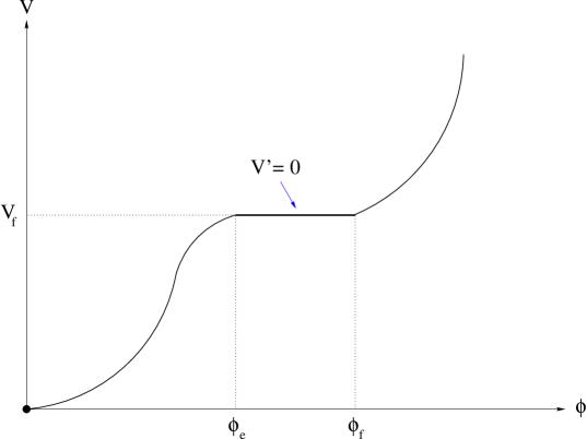
Figure 4: The scalar potential associated with a phase of ultra slow roll inflation.                       In the region $\varphi_{e}\leq\varphi\leq\varphi_{f}$ the potential is exactly flat with value $V_{f}$.

In the flat region all derivatives of the potential vanish, so all of the slow roll parameters are zero. Although the scalar is rolling ever more slowly – hence the name – this is a situation in which the conventional slow roll approximation completely breaks down. In fact the slow roll prediction (119) for the scalar power spectrum actually diverges! The difficulty of reconciling this with a system which is approaching a pure de Sitter phase was the occasion of much reflection by Grishchuk [27]. We shall see that ${\cal P}_{\rm SW}(k)$ is finite, but that it can become quite large.

By adding the background Einstein equations (35-36) and then substituting (143) one finds:

$$1+q(t)\;=\;4\pi G\;\frac{\dot{\varphi}_{0}^{2}}{H^{2}}\;=\;4\pi G\;\Biggl{(}\frac{\dot{\varphi}_{f}}{H(t)}\Biggr{)}^{2}\,\Biggl{(}\frac{a_{f}}{a(t)}\Biggr{)}^{6}\;\;.$$ (145)

During inflation the deceleration parameter is typically near $-1$, but the fact that it approaches this value exponentially fast during the ultra slow roll phase makes a crucial change in the parameter $r(t)$ defined in (39):

$$r(t)\;\equiv\;\frac{1}{H}\;\frac{d}{dt}\ln\Bigl{(}\sqrt{1+q}\,\Bigr{)}\;=\;-3-\frac{\dot{H}}{H^{2}}\;=\;-2+q(t)\;\;.$$ (146)

Although $r(t)$ is near zero for typical models of inflation, we see that it is nearly $-3$ during the ultra slow roll phase. It is simple enough to obtain an exact expression as well for its derivative during this phase:

$$\frac{\dot{r}}{H}\;=\;\frac{\dot{q}}{H}\;=\;2(1+q)\times\frac{1}{2H}\,\frac{\dot{q}}{1+q}\;=\;-2(2-q)(1+q)\;\;.$$ (147)

Note that this quantity is nearly zero, both for typical inflation and during ultra slow roll phase.

It is now straightforward to evaluate our factor ${\cal C}_{1C}(k)$ that depends upon the system’s state at horizon crossing. Substituting in (105) gives the following result during the ultra slow roll phase:

$$q_{C}(t)\;=-\frac{q}{q-1}-\frac{2(2-q)(1+q)}{(q-1)^{2}}\;=\;1+\frac{1}{q-1}-\frac{4}{(q-1)^{2}}\;\;.$$ (148)

Although $q_{C}(t)\simeq+1$ in typical models of inflation, we see that it rapidly approaches $-\frac{1}{2}$ during the ultra slow roll phase. Evaluating (106) for $q_{1C}=-\frac{1}{2}$ and $r_{1}=-3$ gives:

$${\cal C}_{1C}(k)\,\Bigg{|}_{\,r_{1}\,=\,-3}^{\,q_{1C}\,=\,-\frac{1}{2}}\;=\;\frac{1}{4\sqrt{\pi}}\;\Gamma\Bigl{(}-\frac{3}{2}\Bigr{)}\;=\;\frac{1}{3}\;\;.$$ (149)

To estimate the evolution-dependent factor ${\cal C}_{iC}(k)$ we make the reasonable assumption that the system goes suddenly from $q_{C}\simeq+1$ to $q_{C}\simeq-\frac{1}{2}$. In this case the transfer matrix is determined by matching the mode functions and their first time derivatives at the onset of the flat region:

$$\Bigl{(}-iJ_{-\frac{5}{2}}(-x_{f})\,,\,J_{\frac{5}{2}}(-x_{f})\Bigr{)}\left(\matrix{{\cal M}_{C}^{11}&{\cal M}_{C}^{12}\cr{\cal M}_{C}^{21}&{\cal M}_{C}^{22}}\right)\!\! = \!\!\Bigl{(}iJ_{\frac{1}{2}}(-x_{f})\,,\,J_{-\frac{1}{2}}(-x_{f})\Bigr{)},$$ (150)

$$\Bigl{(}-iJ^{\prime}_{-\frac{5}{2}}(-x_{f})\,,\,J^{\prime}_{\frac{5}{2}}(-x_{f})\Bigr{)}\left(\matrix{{\cal M}_{C}^{11}&{\cal M}_{C}^{12}\cr{\cal M}_{C}^{21}&{\cal M}_{C}^{22}}\right)\!\! = \!\!\Bigl{(}iJ^{\prime}_{\frac{1}{2}}(-x_{f})\,,\,J^{\prime}_{-\frac{1}{2}}(-x_{f})\Bigr{)}.\;\;\;\;\;\;\;\;$$ (151)

The matrix elements needed for the scalar power spectrum are:

$${\cal M}_{C}^{21} = \frac{i\pi\,x_{f}}{2}\,\Bigl{[}\,-J_{-\frac{5}{2}}(-x_{f})\,\,J^{\prime}_{\frac{1}{2}}(-x_{f})\;+\;J^{\prime}_{-\frac{5}{2}}(-x_{f})\,\,J_{\frac{1}{2}}(-x_{f})\,\Bigr{]}\;\;,$$ (152)

$${\cal M}_{C}^{22} = \frac{\pi\,x_{f}}{2}\,\Bigl{[}\,-J_{-\frac{5}{2}}(-x_{f})\,\,J^{\prime}_{-\frac{1}{2}}(-x_{f})\;+\;J^{\prime}_{-\frac{5}{2}}(-x_{f})\,\,J_{-\frac{1}{2}}(-x_{f})\,\Bigr{]}\;\;.\qquad$$ (153)

Substituting in (133) with $q_{iC}=+1$ we obtain:

$${\cal C}_{iC}(k) = {\cal M}^{21}_{C}\,+\,{\cal M}^{22}_{C}\;\;,$$ (154)

$$= \sqrt{\frac{\pi x_{f}}{2}}\;e^{-ix_{f}}\,\Biggl{\{}-\Biggl{[}\,1-\frac{i}{2x_{f}}\,\Biggr{]}\,J_{-\frac{5}{2}}(-x_{f})\,-\,i\,J^{\prime}_{-\frac{5}{2}}(-x_{f})\Biggr{\}}\;\;,\qquad$$ (155)

$$= -1+\frac{3}{x_{f}}+\frac{3i}{x_{f}^{2}}-e^{-ix_{f}}\,\Biggl{\{}\frac{3}{x_{f}^{2}}\sin(x_{f})+\frac{6}{x_{f}^{3}}\cos(x_{f})\Biggr{\}}\;\;.$$ (156)

Because first horizon crossing occurs after the scalar has rolled onto the flat region we can assume $x_{f}>1$. It is not safe to assume $x\gg 1$ because some modes will experience horizon crossing soon after the ultra slow roll phase begins. The power spectrum of these modes will deviate much more from scale invariance than is typically the case. Although the flat region must be narrow enough that the scalar can roll across, this process can be tuned to require an arbitrarily long time. For modes which experience horizon crossing long after the onset of the ultra slow roll phase, one can assume $x_{f}\gg 1$, in which case:

$$x_{f}\gg 1\quad\Longrightarrow\quad\|\,{\cal C}_{iC}(k)\,\|^{2}\;\simeq\;1\;\;.$$ (157)

We constructed this model as an exotic system in which the slow roll paradigm completely breaks down. However, it has two other properties worthy of note. The first is that, although our prediction (117) for the scalar power spectrum remains finite, it can become quite large owing to the inverse factor of $(1+q_{1})$. We have seen from (145) that $(1+q(t))$ approaches zero exponentially fast. It seems inevitable that back-reaction must eventually become significant if the ultra slow roll phase is protracted.

The second interesting property of this model is that the anisotropies generated during the ultra slow roll phase are entirely due to scalar kinetic energy. The potential is completely flat so the only possible fluctuations derive from the gravitational response to kinetic energy. This is usually dismissed as negligible but we have just seen that it can drive an enormously strong effect as the system approaches de Sitter inflation. This suggests that one might expect a similarly strong effect from gravitons – the combination of two of which can produce a scalar – if the computation were carried to next order in the weak field expansion.

References

[1] V. F. Mukhanov and G. V. Chibisov,
JETP Lett. 33 (1981) 532.
[2] S. W. Hawking,
Phys. Lett. B115 (1982) 295.
[3] A. H. Guth and S. Y. Pi,
Phys. Rev. Lett. 49 (1982) 1110.
[4] A. A. Starobinskiĭ,
Phys. Lett. B117 (1982) 175.
[5] V. Mukhanov, H. Feldman and R. Brandenberger,
Phys. Rep. 215 (1992) 203.
[6] A. R. Liddle and D. H. Lyth,
Phys. Rep. 231 (1993) 1,
arXiv:astro-ph/9303019.
[7] J. E. Lidsey, A. R. Liddle, E. W. Kolb,
E. J. Copeland, T. Barreiro and M. Abney,
Rev. Mod. Phys. 69 (1997) 373,
arXiv:astro-ph/9508078.
[8] D. N. Spergel et al.,
Astrophys. J. Suppl. 148 (2003) 175,
arXiv:astro-ph/0302209.
[9] H. V. Peiris et al.,
Astrophys. J. Suppl. 148 (2003) 213,
arXiv:astro-ph/0302225.
[10] N. C. Tsamis and R. P. Woodard,
Class. Quant. Grav. 20 (2003) 5205,
arXiv:astro-ph/0205331.
[11] N. C. Tsamis and R. P. Woodard,
Class. Quant. Grav. 21 (2003) 93,
arXiv:astro-ph/0306602.
[12] E. D. Stewart and D. H. Lyth,
Phys. Lett. B302 (1993) 171,
arXiv:gr-qc/9302019.
[13] L. Wang, V. F. Mukhanov and P. J. Steinhardt,
Phys. Lett. B414 (1997) 18.
arXiv:astro-ph/9709032.
[14] J. Martin and D. J. Schwarz,
Phys. Rev. D62 (2000) 103520.
arXiv:astro-ph/9911225.
[15] E. D. Stewart and J. Gong,
Phys. Lett. B510 (2001) 1,
arXiv:astro-ph/0101225.
[16] D. J. Schwarz, C. A. Terrero-Escalante and A. A. Garcia,
Phys. Lett. B517 (2001) 243,
arXiv:astro-ph/0106020.
[17] S. Habib, K. Heitmann, G. Jungman and C. Molina-Paris,
Phys. Rev. Lett. 89 (2002) 281301,
arXiv:astro-ph/0208443.
[18] J. Martin and D. J. Schwarz,
Phys. Rev. D67 (2003) 083512,
arXiv:astro-ph/0210090.
[19] S. M. Leach, A. R. Liddle, J. Martin and D. J. Schwarz,
Phys. Rev. D66 (2002) 023515,
arXiv:astro-ph/0202094.
[20] R. K. Sachs and A. M. Wolfe,
Astrophys. J., 147 (1967) 73.
[21] J. Iliopoulos, T. N. Tomaras, N. C. Tsamis
and R. P. Woodard,
Nucl. Phys. B534 (1998) 419,
arXiv:gr-qc/9801028.
[22] L. R. Abramo and R. P. Woodard,
Phys. Rev. D65 (2002) 063515,
arXiv:astro-ph/0109272.
[23] A. A. Starobinskiĭ,
JETP Lett. 30 (1979) 682.
[24] V. A. Rubakov, M. V. Sazhin and A. V. Veryaskin,
Phys. Lett. B115 (1982) 189.
[25] R. Fabbri and M. D. Pollock,
Phys. Lett. B125 (1982) 445.
[26] A. A. Starobinskiĭ,
Sov. Astron. Lett. 11 (1985) 133.
[27] L. P. Grishchuk,
Phys. Rev. D50 (1994), 7154,
arXiv:gr-qc/9405059.