H.E.S.S. contributions to the
28th International Cosmic Ray Conference
Tsukuba, Japan

Contents

1. Status of the H.E.S.S. Project 5

2. Performance of the H.E.S.S. cameras. 9

3. Observation Of Galactic TeV Gamma Ray Sources
   With H.E.S.S. 13

4. First Results from Southern Hemisphere AGN Observations
   Obtained with the H$\cdot$E$\cdot$S$\cdot$S$\cdot$ VHE Gamma-ray Telescopes 17

5. Study of the Performance of a Single Stand-Alone H.E.S.S. Telescope: Monte Carlo Simulations and Data 21

6. Application of an analysis method based on a semi-analytical
   shower model to the first H$\cdot$E$\cdot$S$\cdot$S$\cdot$ telescope. 25

7. The Central Data Acquisition System of the
   H.E.S.S. Telescope System 29

8. Mirror alignment and performance of the optical system of the H.E.S.S. imaging atmospheric Cherenkov telescopes 33

9. Calibration results for the first two H$\cdot$E$\cdot$S$\cdot$S$\cdot$ array telescopes. 37

10. Arcsecond Level Pointing Of The H.E.S.S. Telescopes 41

11. A Novel Alternative to UV-Lasers Used in Flat-fielding
    VHE $\gamma$-ray Telescopes 45

12. Atmospheric Monitoring For The H.E.S.S. Project 49

13. Implications of LIDAR Observations at the H.E.S.S. Site in
    Namibia for Energy Calibration 53

14. Optical Observations of the Crab Pulsar using the first H.E.S.S. Cherenkov Telescope 57

Chapter 1 Status of the H.E.S.S. Project

Werner Hofmann, for the H.E.S.S. collaboration
Max-Planck-Institut für Kernphysik, D 69029 Heidelberg, P.O. Box 103989

Abstract

H.E.S.S. - the High Energy Stereoscopic System - is a system of four large imaging Cherenkov telescopes under construction in the Khomas Highland of Namibia, at an altitude of 1800 m. With their stereoscopic reconstruction of air showers, the H.E.S.S. telescopes provide very good angular resolution and background rejection, resulting in a sensitivity in the 10 mCrab range, and an energy threshold around 100 GeV. The H.E.S.S. experiment aims to provide precise spectral and spatial mapping in particular of extended sources of VHE gamma rays, such as Supernova remnants. The first two telescopes are operational and first results are reported; the next two telescopes will be commissioned until early 2004.

1. The H.E.S.S. Telescopes

The H.E.S.S. Cherenkov telescopes are characterized by a mirror area of slightly over 100 m², with a focal length of 15 m, and use cameras with fine pixels of $0.16^{\circ}$ size and a large field of view of $5^{\circ}$.

Construction of telescopes is well underway; the steel structures of all four telescopes have been erected and equipped with drive systems; two telescopes are fully equipped with mirrors and cameras and take data since June 2002 and March 2003, respectively. The final two telescopes will be commissioned early in 2004; all parts, such as mirrors, phototubes etc. are in hand, and the cameras are under assembly in France. The site infrastructure is complete and includes a building with the experiment control room, offices, and workshops, a residence building, Diesel power generators and a Microwave tower linking the site to Windhoek and from there to the internet.

The H.E.S.S. telescopes use an alt-az mount, which rotates on a 15 m diameter rail. The steel structures are designed for high mechanical rigidity. Both azimuth and elevation are driven by friction drives acting on auxiliary drive rails, providing a positioning speed of $100^{\circ}$/min. Encoders on both axes give 10” digital resolution; with the additional analogue encoder outputs, the resolution is improved by another factor 2 to 3. After initial tests and a few months of operation of the first telescope, the drives were slightly modified for smoother operation; the telescope design is now quite mature.

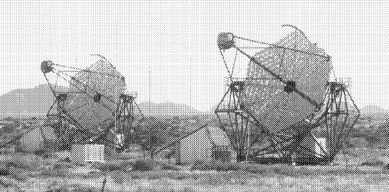
Fig. 1.: The first two H.E.S.S. telescopes, ready to take data.

The mirror of a H.E.S.S. telescope is composed of 380 round facets of 60 cm diameter; the facets are made of ground glass, aluminized and quartz coated, with reflectivities in the 80% to 90% range. The facets are arranged in a Davies-Cotton fashion, forming a dish with 107 m² mirror area, 15 m focal length and $f/d\approx 1.2$. To allow remote alignment of the mirrors, each mirror is equipped with two alignment motors with internal resolvers. The alignment procedure uses the image of a star on the closed lid of the PMT camera, viewed by a CCD camera at the center of the dish. The procedure and the resulting point spread function are described in detail elsewhere in these proceedings. Due to the superior quality of both the mirrors and the alignment system, the on-axis point spread function is significantly better than initially specified. The imaging quality is stable over the elevation range from $30^{\circ}$ to the Zenith. The point spread function varies with distance $\theta$ (in degr.) to the optical axis as $r_{80}=(0.42^{2}+(0.71\theta)^{2})^{1/2}~{}~{}~{}\mbox{[mrad]}$; $r_{80}$ is the circle containing 80% of the light of a point source at the height of the shower maximum. Over most of the field of view, light is well contained within a single pixel.

Telescope pointing was verified using the images of stars on the camera lid. Without any corrections, star images were centred on the camera lid with a rms error of 28”. Using a 12-parameter model to correct for misalignments of the telescopes axes etc., a pointing precision of 8” rms is reached. Finally, using a guide telescope attached to the dish for further corrections, the pointing can be good to 2.5” rms. H.E.S.S. should therefore be able to locate gamma ray sources to a few arc-seconds.

The PMT cameras of the H.E.S.S. telescopes provide $0.16^{\circ}$ pixel size over a $5^{\circ}$ field of view, requiring 960 PMT pixels per telescope. The complete electronics for signal processing, triggering, and digitization is contained in the camera body; only a power cable and a few optical fibers connect the camera. For ease of maintenance, the camera features a very modular construction. Groups of 16 PMTs together with the associated electronics form so-called “drawer” modules, 60 of which are inserted from the front into the camera body, and have backplane connectors for power, a readout bus, and trigger lines. The rear section of the camera contains crates with a PCI bus for readout, a custom crate for the final stages of the trigger, and the power supplies. The camera uses Photonis XP2960 PMTs, operated at a gain of $2\times 10^{5}$. The PMTs are individually equipped with DC-DC converters to supply a regulated high voltage to the dynodes; for best linearity, the four last dynodes are actively stabilized.

The key element in the signal recording of the H.E.S.S. cameras is the ARS (Analogue Ring Sampler) ASIC, which samples the PMT signals at 1 GHz and provides analogue storage for 128 samples, essentially serving to delay the signal until a trigger decision is reached. To provide a large linear dynamic range in excess of $10^{4}$ up to 1600 photoelectrons, two parallel high/low gain channels are used for each PMT. A camera trigger is formed by a coincidence of some number of pixels (typically 3-5) within an $8\times 8$ pixel group exceeding an adjustable threshold; typical operating thresholds are in the range of 3 to 5 photoelectrons. The pixel comparators generate a pixel trigger signal; the length of the signal reflects the time the input signal exceeds the threshold. Since typical noise signals barely exceed the threshold and result in short pixel trigger signals, the effective resolving time of the pixel coincidence is in the 1.5 to 2 ns range, providing a high suppression of random coincidences. At the time of this writing, the two telescopes are triggered indepedently, and stereo images are combined offline using GPS time stamps. A central trigger processor controlling electronic delays and coincidence logic will soon be installed. This will allow to impose arbitrary telescope configurations in the trigger, and to operate the telescopes either as a single four-telescope system, or as subsystems, up to four individual telescopes pointed at different objects.

A number of auxiliary instruments serve to monitor telescope performance and atmospheric quality. These include laser and LED pulsers at the center of a dish for flatfielding, and infrared radiometers and a lidar system to detect clouds and characterize aerosol scattering. Details are given elsewhere in these proceedings.

2. First data

After the first telescope was equipped with mirrors in autumn of 2001, the camera was installed in May 2002 and first data were taken in June 2002. As expected for a single telescope, a significant fraction - roughly half - of the images are caused by muons, either in the form of full rings or of short ring segments.

The night-sky background - predicted to be about 100 MHz photoelectron rate per pixel - induces a noise of 1.2 to 1.5 photoelectrons rms in the PMT pixels, consistent with expectations.

Muon rings are used to verify the overall performance and calibration of the telescopes. Rings are classified according to their radius - related to the muon energy - and by the impact parameter, which governs the intensity distribution along the ring. The observed photoelectron yield agrees to better than 15% with expectations, indicating that the optical system, the PMTs and electronics calibration are quite well understood. This tool can be used to monitor the evolution of the detectors, as explained in greater detail in an accompanying paper.

Another important check for the performance of the telescope is the trigger rate. The rate varies smoothly with threshold. Even for thresholds as low as four photoelectrons, trigger rates are governed by air showers rather than by night-sky noise, which would induce a much faster variation with threshold. With a typical threshold of 4-5 photoelectrons, event size distributions peak around 100 to 150 photoelectrons; for the H.E.S.S. telescopes one photoelectron corresponds approximately to one GeV deposited energy.

Objects observed so far include SN 1006, RXJ 1713-3946, PSR B1706-44, the Crab Nebula, and NGC 253, PKS 2005-489, PKS 2155-304 as extragalactic source candidates. Clear signals are detected from the Crab Nebula and for PKS 2155, confirming the earlier detection by the Durham telescopes. The spectral shape of the Crab data agrees well with other measurements; for PKS 2155, a slightly steeper spectrum is measured. Details are given in other contributions to this conference. First stereo data were collected in March 2003, using the first two telescopes with an offline selection of concident events. As expected, muons rings were found to be absent in coincident events. A parallel trigger to retain some muon events when stereo coincidence operation begins is under consideration.

3. Conclusion

The first two H.E.S.S. telescopes are operational since June 2002 and March 2003, respectively, and first results concerning the technical performance of the telescopes, both for the optical system and the camera, look encouraging and did not expose major problems. Current schedules call for completion of the Phase-I four-telescope system in 2004. An expansion of the system - Phase II - with increased sensitivity is foreseen; the Phase II telescopes and their arrangement are under study.

Acknowledgement

Construction and operation of the H.E.S.S. telescopes is supported by the German Ministry for Education and Research BMBF.

Chapter 2 Performance of the H.E.S.S. cameras.

P. Vincent¹, J.-P. Denance¹, J.-F. Huppert¹, P. Manigot², M. de Naurois², P. Nayman¹, J.-P. Tavernet¹, F. Toussenel¹, L.-M. Chounet², B. Degrange², P. Espigat³, G. Fontaine², J. Guy¹, G. Hermann⁴, A. Kohnle⁴, C. Masterson⁴, M. Punch³, M. Rivoal¹, L. Rolland¹, T. Saitoh⁴, for the H.E.S.S. collaboration.
(1) LPNHE, IN2P3/CNRS Universités Paris VI & VII, Paris, France
(2) LLR, IN2P3/CNRS Ecole Polytechnique, Palaiseau, France
(3) PCC, IN2P3/CNRS College de France, Paris, France
(4) Max Planck Institut fuer Kernphysik, Heidelberg, Germany

1. Introduction

The H.E.S.S. experiment is a new generation ground-based atmospheric Cherenkov detector. The first phase of this experiment consists of a square array of four telescopes with 120-metre spacing. Each telescope, equipped with a mirror of 107 m², has a focal plane at 15 metres where a camera is installed. Each camera consists of 960 photo-multipliers (PMs), providing a total field of view of 5^∘, with the complete acquisition system (analogue to digital conversion, read-out, fast trigger, on-board acquisition) being contained in the camera. The cameras of the H.E.S.S. telescopes are currently being installed in the Khomas highlands, Namibia. The first telescope has been taking data since June, 2002 and the second since February, 2003. Stereoscopic coincient trigger mode should begin in June, 2003 and full Phase I operation should be underway early in 2004. The performance of the cameras will be presented and their characteristics as measured during data taking will be compared with those obtained during the construction phase using a test bench. Future upgrades based on experience operating the two first cameras are also discussed.

2. The cameras of the H.E.S.S. telescopes.

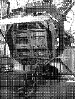
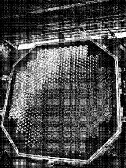
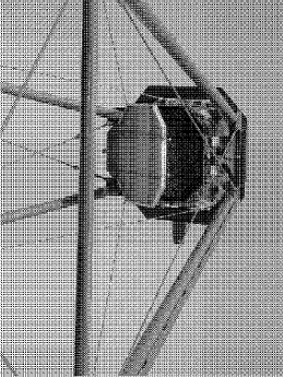
Fig. 1.: View of the second H.E.S.S. camera. The picture on the left shows the rear with the four power supplies, the mixed crate incorporating the custom bus and compact PCI bus, and the network interface. The central picture shows the front side of the camera with lid open showing the 960 Winston cones. On the right we see the camera on the telescope.

A camera is approximately octagonal, fitting in a cylinder 2 metres in length and 1.6 metres in diameter, and weighing about 900 kg (see Fig. 1). The front part contains 60 interchangable modules (“drawers”) with 16 PMs each, lodged in a “pigeon-hole” plate. The drawers are held by only two screws and can be easily extracted from the body of the camera to be replaced by a new drawer. Each drawer communicates with the rest of the electronics through three connectors at the rear, which plug in automatically when drawers are installed. This conception allows an easy access for tests and repairs of the camera electronics. In front of the drawers, a plate in three sections holds individual Winston cones for each PM which concentrate the Cherenkov light in the central region of the photo-cathode where the quantum efficiency is at a maximum of about 30%. These cones allow the collection of about 75% of the photons reflected from the mirror. They also considerably reduce the background contribution from albedo by limiting the PM’s field of view to the angular size of the mirror. In the rear of the camera, an electronics rack is equipped with four power-supply crates, the camera acquisition and control systems, and the network interface. This rack can be slid out on rails from the camera body to access the cables and connectors between front and back side of the camera. Lastly, only three cables come from the camera to the ground: a copper cable for the current, one optical fibre for the network, and an other fibre for communications with central trigger.

3. The electronics.

The electronics of the camera consist of a front-end contained in the drawers which includes the readout and first-level trigger and a second section with the local acquisition system mentioned above. Drawers contain 16 PMs, each powered by an active base. These bases provide a high voltage of more than a thousand volts calibrated to generate a signal of $2\times 10^{5}$ electrons for each photon converted at the photo-cathode. The PMs use a borosilicate window and provide a 20–30% quantum efficiency in the wavelength range 300–700 nm.

The readout channel takes advantage of analogue memories ARS0 (“Analog Ring Sampling memory”) developed for the ANTARES experiment by the CEA/DAPNIA-SEI. These memories sample the signal at 1 GHz and store it in 128 cells while awaiting the trigger decision. The pulse from each PM is divided between two channels with different amplification factors. A high-gain channel, for low signal amplitudes, gives a dynamic range from 1 to about 100 photo-electrons. Before this upper limit, at around 16 photo-electrons, the low gain channel can measure a signal up to 1600 photo-electrons. The overlapping region allows inter-calibration between both channels. The signal from a triggered event is read from the analogue memory in a window of 16 samples and then digitized with a 12-bit ADC and stored in an FPGA chip. The samples can be saved for an analysis of the pulse shape or integrated directly in the FPGA so as to transmit and save only the total charge in a pixel. The readout-window size is a programmable parameter that can be changed as a function of future studies.

The local camera trigger is based on two parameters: the number of photons arriving in a pixel and the identification of a concentration of signal in a part of the camera. To construct the latter criterion the camera has been divided in 38 sectors of 64 PMs with logic on cards contained in the rear crate. Sectors overlap with their neighbours to prevent local inhomogeneities which would result from a shower image arriving in the boundary between two sectors. The time needed to build the trigger signal is about 70 ns, which is fast enough permit reading of the signal stored in the ARS0. A card dedicated to the trigger management (“GesTrig”) sends a signal through two fanout cards to the 480 analogue memories. The memories stop acquiring data, a programmable pointer identifies the region of interest given the trigger-signal formation time, and the readout of the data starts. The time until the converted signals are ready in the drawers’ FPGAs is measured to be 270$\>\mu$s after the shower’s arrival, and is remarkably stable.

The interface with central trigger of the multi-telescope system is performed via a local module embedded in the camera. This central trigger interface is connected to the GesTrig trigger manager card and informs the central trigger of the current status of the camera with a “busy” signal. If there is no coincidence with other telescopes, the central trigger returns a “fast clear” within a couple of $\>\mu$s, which is sent to the GesTrig and thence to the drawers to stop the readout of the analogue memories and to reset the drawers.

4. Data acquisition architecture and performance

The acquisition system is based on the use of the new Compact-PCI (cPCI) norm that allows 64-bit word transfer at 33 MHz. A second bus (CustomBUS) within the data acquisition crate is dedicated to the configuration of the sectorization of the trigger. The drawers are connected to the acquisition by 4 final buses (Box-Bus), and when an event is available for transfer they send a request to a card holding FIFO memories (FIFO-card) located on the cPCI bus. This card plays the rôle of master and controls the transactions on the 4 buses by sending acknowledges to slaves (drawers). All buses accept asynchronous transfer, and the full data transfer from the 15 drawers present on each bus is completed after $340\>\mu$s. This year, the RIOC-4065 processor from CES has been installed on the first two cameras. This new processor is able to perform direct access between a card in the cPCI bus and its own memory and so improve the performance of the acquisition. The FIFO memories are read-out through the cPCI bus by a DMA chip that transfers the full camera’s data in less than $140\>\mu$s. This last time, together with the bus transfer time and the ARS conversion time of the previous section, defines the dead-time of the acquisition. As the readout time of the FIFO memory is lower than the other times, this task can be parallelized so that the dead-time for a camera is $610\>\mu$s, corresponding to a maximum acquisition rate of 1.6 kHz which represents an improvement of a factor of three from the initial camera’s performance. Under these conditions, at a typical trigger configuration of 4 pixels at 5 photo-electrons, the observed counting rate is 250 Hz. This rate gives a dead-time of about 14%, compared to 30% with the initial camera.

The data acquisition system (DAS) in the camera is build around the Linux operating system and written in C. This system controls the behaviour of the overall camera: one card controls the camera lid operation, the 95 fans and 16 temperature sensors; a GPS card for time stamps receives interruptions from the GesTrig trigger card; a CAN bus interface controls the four power-supply crates; an I/O card manages the trigger; a mezzanine card located on the CustomBUS receives some serial event data the from central trigger interface (event number …). Data are transfered from the local CPU to the central DAS via a 100 Mbits/s network for conversion and storage in ROOT format.

5. Conclusion.

Since the installation of the first camera “prototype” several upgrades have been carried out. Experimentally we had strong indications that noise from the switching power-supplies considerably disturbed the data “traffic” on the BoxBus. The buses on new camera have been modified to remedy this problem and the first prototype has been upgraded accordingly. Other upgrades are under study to further increase the acquisition speed, e.g., to double the number of Box-buses to gain a further factor two in the data transfer. Finally, some tests on DMA transfer may allow the FIFO memory readout time to be reduced to $60\>\mu$s. This would not decrease dead time but would leave the CPU free to perform, for example, other monitoring tasks or data compression (zero-suppression). In conclusion, the performance of the first two cameras for the Phase I of H.E.S.S. is promising and, and are undergoing continual upgrades in order to optimize performance.

Chapter 3 Observation Of Galactic TeV Gamma Ray Sources With H.E.S.S.

Conor Masterson¹, for the H.E.S.S. Collaboration²
(1) MPI fuer Kernphysik, P.O. Box 103980, D-69029 Heidelberg, Germany
(2) http://www.mpi-hd.mpg.de/HESS/collaboration

Abstract

The first telescope of the H.E.S.S. stereoscopic Cherenkov telescope system started operation in summer 2002. In spring 2003 a second telescope was added, allowing stereoscopic observations. A number of known or potential TeV gamma-ray emitters in the southern sky were observed. Data on the Crab nebula taken at large zenith angles show a clear signal and serve to verify the performance and calibration of the instrument. Observations of other Galactic sources are also summarized.

1. Introduction

The H.E.S.S. experiment commenced operations on-site in Namibia in June, 2002, with the first of four Cherenkov telescopes. With its high resolution camera (0.16^∘ pixel size) and large mirror area (107 m²) the single H.E.S.S. telescope is a sensitive instrument in its own right, comparing favourably with existing detectors. The large field of view of the detector, ($\approx 5^{\circ}$) makes it a good choice for observations of extended galactic objects. Observations were made of a number of candidate $\gamma$-ray sources with the single telescope, pending the installation of the rest of the array. These sources included the Crab nebula, an established TeV source, as well as a number of other Galactic sources.

The Crab nebula was discovered at TeV energies in 1989 [6] and is conventionally used as a standard reference source of TeV $\gamma$-rays, due to its relative stability and high flux. It was observed with the first telescope in October and November 2002 for a total of 4.65 hours (live-time). Due to the latitude of the H.E.S.S. experiment (21^∘ South), observations were taken over a zenith angle range of 45^∘ to 50^∘.

2. Analysis of Data

Since the data reported in this paper were taken with the first H.E.S.S. telescope operating in single telescope mode, a standard analysis of type Supercuts [5] was applied in order to extract a $\gamma$-ray signal. This uses simple selection criteria based on parameters calculated from the moments of the Cherenkov images.

Data were taken in ON-OFF observation mode, with 25-minute observations of the source accompanied by similar observations of a control region offset by 30 minutes in Right Ascension from the source. In order to calibrate the system, a number of artificial light sources are used, including an array of light emitting diodes on the inside of the camera lid. These LEDs are used to measure the single photo-electron gain of the system. Also, a laser mounted on the dish allows flat-fielding of the camera [3].

Images were cleaned using a two-step technique, requiring pixels in the image to be above a lower threshold of 5 photo-electrons and to have a neighbour above 10 photo-electrons. Second-moment parameters were calculated for each cleaned image using the Hillas [1] definitions and these parameters were used to select candidate $\gamma$-ray events. The selection criteria were optimized using Monte-Carlo simulated $\gamma$-ray showers and real background runs at the same zenith angle range as the observations. The selection cuts are summarized in table 1, a diagram illustrating the parameter definitions is shown in figure 1.

Parameter	Cut
Length	4.8	mrad
Width (lower)	0.05	mrad
Width (upper)	1.3	mrad
Length/Amp.	0.016	mrad/p.e.
Distance	17.0	mrad
$\alpha$	9.0	deg.

Table 1.: Optimized $\gamma$-ray selection criteria.

Fig. 1. Definition of Hillas Parameters

3. Results

The data from the Crab nebula observations have been analysed using the above technique, giving a steady rate of 3.6 $\gamma\ \textrm{min}^{-1}$ with a significance of 20.1 $\sigma$ after applying the above-mentioned selection cuts. The $\alpha$ parameter distributions for the ON and OFF data are shown in Figure 2. The two-dimensional skyplot is shown in figure 3. The source reconstruction for the skyplot uses a simple single telescope source reconstruction scheme based on Hillas parameters [4].

Fig. 2. Alpha plot, 2d plot of $\gamma$-ray excess from the Crab nebula, the OFF data is normalized to take account of the exposure time differences.

Fig. 3. Reconstructed skyplot of $\gamma$-ray excess in mrad around the source position

The effective area for $\gamma$-rays has been estimated for one of the Monte Carlo simulations described in the accompanying article using the above selection cuts. The pre- and post-selection effective area distributions as a function of the true Monte Carlo input energy are shown in figure 4 for simulated $\gamma$-rays at a zenith angle of $45^{\circ}$. The differential $\gamma$-ray rate for a source with a spectrum similar to that of the Crab is given in figure 5. It can be seen that the energy threshold after the above selection cuts, as defined by the peak in the differential rate distribution, is 780 GeV. The energy threshold before selection cuts is 590 GeV. The fixed cuts on Hillas parameters described reject most $\gamma$-rays at high energies, this may be remedied by varying the cuts with image amplitude, which is currently under study.

Fig. 4. Effective areas before and after selection cuts as a function of true simulated energy

Fig. 5. Differential rate for a source with a spectrum similar to the Crab at $45^{\circ}$ zenith angle.

A preliminary estimation of the integral flux based on one of the Monte Carlo simulations gives a value of $(2.64\pm 0.20)\times 10^{-7}$ m^-2 s^-1 ($>1$ TeV), for which the quoted error include only the statistical errors; no systematic errors are included. Preliminary analysis of the spectral energy distribution indicates that the signal follows a power-law form with a slope not inconsistent with measurements by other instruments. Uncertainties in the energy threshold and spectral analysis are in large part due to differing estimates of the collection efficiency for $\gamma$-rays from different Monte Carlo simulations, which is the subject of ongoing study.

4. Observations of other Galactic Sources

Observations were made of a number of other Galactic sources with the first H.E.S.S. telescope during 2002 and early 2003, calibration and analysis of these data will be presented in the talk accompanying this paper. Observations are summarized in table 2, with live time corrected exposures on the sources and the mean zenith angle of the observation. The remaining Crab data is currently under analysis.

Source	Obs. Time (hrs)	Mean Zenith Angle (∘)	Type
Crab (total)	14.2	47.7	Plerion
Vela	22.4	28.6	Plerion
Cen X-3	29.6	38.27	X-Ray Binary
SN1006	41.0	23.6	SNR
Vela Jr	1.2	24.9	SNR
RXJ 1713	1.2	16.7	SNR

Table 2.: Summary of galactic Source Observations up to beginning May 2003

5. Conclusions

A strong signal has been detected from the Crab nebula during the first few months of operation of the first H.E.S.S. instrument. Preliminary work suggests that the spectral slope is consistent with measurements from other instruments, while the absolute flux normalization is the subject of further study. The second telescope of the H.E.S.S. system has been commissioned and stereo observations have commenced. Calibration and analysis of data taken in stereo mode will also be reported on in the talk accompanying this paper.

6. References

1. Hillas A. 1985, in Proc. 19nd I.C.R.C. (La Jolla), Vol. 3, p. 445.

2. Konopelko A. et al., These Proceedings.

3. Leroy N. et al., These Proceedings.

4. Lessard R. W. et al., 2001, Astroparticle Physics, 15, 1.

5. Punch M. 1991, in Proc. 22nd I.C.R.C. (Dublin), Vol. 1, p. 464.

6. Weekes T. C. et al. 1989, Astrophysical Journal, 342, 379 (1989).

Chapter 4 First Results from Southern Hemisphere AGN Observations Obtained with the H$\cdot$E$\cdot$S$\cdot$S$\cdot$ VHE Gamma-ray Telescopes

A.Djannati-Ataï¹, for the H$\cdot$E$\cdot$S$\cdot$S$\cdot$ collaboration².
(1) PCC-IN2P3/CNRS College de France Université Paris VII, Paris, France
(2) http://www.mpi-hd.mpg.de/HESS/collaboration

Abstract

The first and second telescopes of the H$\cdot$E$\cdot$S$\cdot$S$\cdot$ stereoscopic system are operating since June 2002 and February 2003, respectively. We will present the first results from a number of southern AGN observed using the first two H$\cdot$E$\cdot$S$\cdot$S$\cdot$ telescopes, which already yield a significant sensitivity in mono-telescope mode, with a threshold for detection below that of other Imaging Atmospheric Cherenkov Telescopes. In this paper we report in particular on the first detection of an AGN by H$\cdot$E$\cdot$S$\cdot$S$\cdot$: the BL Lac object PKS 2155-304 was seen during July and October 2002 at a total significance level of 11.9 standard deviations (s.d.).

1. Introduction

The BL Lac object PKS 2155-304 is one of the brightest nearby blazars ($z=0.116$) in the optical to X-ray range, and is a highly variable source. Numerous multi-wavelength observations (see e.g. [3]) have clearly shown the synchrotron nature of its emission which extends up to hard X-rays (e.g., see results from BeppoSax [2]). As its peak synchrotron frequency lies at UV/soft X-rays, PKS 2155-304 is classified as a High frequency-peaked BL Lac object or HBL [4].

PKS 2155-304 was first seen in the GeV $\gamma$-ray range by the EGRET detector [10] aboard the satellite C-GRO, exhibiting a hard spectrum with a differential index of $1.71\pm 0.24$. It was thereby considered as a strong potential TeV source, despite its redshift for which estimations of the Extragalactic Background Light (EBL) absorption effects are significant. Chadwick et al. [1] reported its first detection in the TeV range with the Mark 6 telescope at Narrabri (Australia) at a level of 6.8 s.d. and a flux above 300 GeV of $4.2\pm 2.1\times 10^{-11}\>\mathrm{cm^{-2}\>s^{-1}}$.

We report here on observations made during July and October 2002 on PKS 2155-304 by the first H$\cdot$E$\cdot$S$\cdot$S$\cdot$ atmospheric Cherenkov telescope operating at a threshold energy of $\sim 150\>\mathrm{GeV}$. Its Davies-Cotton reflector has a focal length of 15 metres and an f/d of $1.2$. It is made up of 380 60 cm diameter mirror facets, giving an effective reflecting area of $107\>\mathrm{m^{2}}$. The camera is equipped with 960 PMs with a pixel size of $0.16{{}^{\circ}}$ for a full field of view of $\sim 5{{}^{\circ}}$ (see [6,11]). The data-set and the analysis technique are presented in the next section. The results and detected signal are then given, and we conclude with a short discussion.

2. Data-set and Analysis

Observations of PKS 2155-304 started shortly after the first H$\cdot$E$\cdot$S$\cdot$S$\cdot$ telescope became operational in June 2002. The data-set used here consists of 7 pairs of ON$-$OFF observation runs (ON being at the source position, and OFF at a control region displaced in Right Ascension) taken during four nights from July 15^th to 18^th, 2002, and 15 pairs taken from September 29^th to October 10^th, 2002, for an ON live-time of 2.18 and 4.7 hours, respectively.

Raw data, consisting of images of cosmic-ray showers, muons, and candidate $\gamma$-rays are first processed through a calibration chain, including pedestal subtraction, ADC-to-photoelectron (p.e.) gain scaling, flat-fielding, bad-channel filtering and image-cleaning (see [7]). Image shape and orientation parameters, obtained after a simple moments analysis [5] are then used to discriminate against the cosmic-ray background. The parameters retained for this discrimination are the length (L), width (W), distance (D), the ratio of the length to the charge in the image (LoverS or L/S), and the pointing angle, $\alpha$ — which is the angle at the image barycentre between the actual source position and the reconstructed image axis of the $\gamma$-ray candidate.

The cut values given in Table 1 were determined through an optimisation procedure where a simulated $\gamma$-ray spectrum with a differential index of $-2.8$ was tested against real background events (available from OFF-source runs). Simulated $\gamma$-ray images were obtained through full Monte Carlo simulations of showers in the atmosphere, and of the telescope response (see [9]).

Table 1.: Cut values: L, W and D are in mrad, L/S in mrad/p.e. and $\alpha$ in degrees.

Parameter	L	W	D	L/S	$\alpha$
Upper cut	5.8	1.42	17	0.017	8∘

The $\gamma$-ray efficiency and the overall background rejection factor obtained using the above cuts are respectively $\epsilon_{\gamma}=25\%$ and $R_{h}\approx 4400$ with a corresponding quality factor $QF=\epsilon_{\gamma}\times\sqrt{R}_{h}$ of 16. Observations of the Crab, with cuts adapted to its low elevation transit, yield a rate of $3.6$  $\gamma\ \textrm{min}^{-1}$ and a significance per hour of 9.3 ([8]).

3. Results

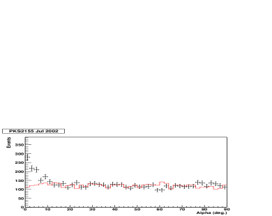
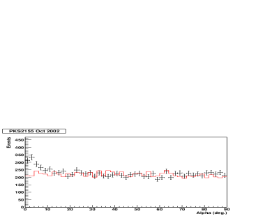
Fig. 1.: The pointing angle $\alpha$-plot of PKS 2155-304 observations for July (left panel) and October (right panel) 2002. The OFF-source distributions have been normalised to the control region between $30{{}^{\circ}}$ and $90{{}^{\circ}}$.

Fig. 1 shows the pointing angle $\alpha$-plots of ON and OFF-source cumulated data after selection cuts for the July and October 2002 data-sets. Excesses of 404 and 337 events, corresponding to $\gamma$-ray rates of 3.1 and 1.2 $\gamma\ \textrm{min}^{-1}$, are observed at significance levels of 9.9 and 6.6 s.d, respectively for the two periods. Hence the TeV flux of PKS 2155-304, as measured by H$\cdot$E$\cdot$S$\cdot$S$\cdot$, decreased significantly over a period of about three months.

Table 2.: Live-time, number of ON and OFF events within the cuts, excess, rate and the significance for July and October 2002.

PKS2155	Ton	Non	Noff	Excess	$\gamma\ \textrm{min}^{-1}$	Significance
Jul 2002	2.2h	1029	625	404	3.1	9.9
Oct 2002	4.7h	1444	1107	337	1.2	6.6

4. Discussion and Conclusion

Observations of PKS 2155-304 by the first H$\cdot$E$\cdot$S$\cdot$S$\cdot$ telescope show a clear signal during July and October 2002, with a total significance of 11.9 s.d., and mark definitely this source into the still-short list of confirmed extragalactic TeV sources, together with Mkn 421 (z=0.031), Mkn 501 (z=0.034), 1ES1959+650 (z=0.048) and 1ES1426+428 (z=0.129).

Comparisons of the detected rates during July, 3.1 $\gamma\ \textrm{min}^{-1}$, and October 2002, 1.2 $\gamma\ \textrm{min}^{-1}$, show a clear dimming of PKS 2155-304 (by a factor $\sim 3$) in the latter period. Although the comparison of the weekly averaged X-ray count-rates for the two periods, as monitored by the All Sky Monitor on board the satellite RXTE, shows a slightly brighter source in July 2002, it has not been possible to make quantitative correlations between the X-rays and $\gamma$-rays due to the very faint flux of the former.

This source, at an intermediate redshift (close to that of 1ES1426+428) in the growing catalogue of extragalactic TeV $\gamma$-ray sources, should provide further information on the link between the intrinsic spectrum of AGN sources and their absorption by the intervening EBL. The H$\cdot$E$\cdot$S$\cdot$S$\cdot$ instrument is well-placed to measure such behaviour, as its low threshold can allow spectral information to be found in the energy region where absorption is almost negligible, while still being sensitive up to the highest $\gamma$-ray energies. An indication of the spectral behaviour, as compared to H$\cdot$E$\cdot$S$\cdot$S$\cdot$ observations on the Crab Nebula, will be presented at the conference as well as results of observations on a number of other AGN which are listed in Table 3.

Table 3.: Other extragalactic sources observed by H$\cdot$E$\cdot$S$\cdot$S$\cdot$

Source	Redshift	ExposureTime	Type
PKS0548-322	0.069	8	BL Lac
1ES1101-232	0.186	6	BL Lac
Mkn 421	0.031	1.6	BL Lac
M87	0.00436	24	NLRG
PKS2005-489	0.071	11	BL Lac

5. References

1. Chadwick, P. M. et al. 1999, ApJ, 513, 161
2. Chiappetti L. et al. 1999, ApJ, 521, 552
3. Edelson R. et al. 1995, ApJ, 438, 120
4. Giommi P., Padovani P. 1995, ApJ, 444, 567
5. Hillas A. 1985, in Proc. 19nd ICRC, 3, 445
6. Hofmann W. et al., These proceedings
7. Leroy N. et al., These proceedings
8. Masterson C. et al., These proceedings
9. Konopelko A. et al., These proceedings
10. Vestrand W.T., Stacy J.G., Sreekumar P. 1995, ApJ, 454, L93
11. Vincent P. et al., These proceedings

Chapter 5 Study of the Performance of a Single Stand-Alone H.E.S.S. Telescope: Monte Carlo Simulations and Data

A. Konopelko,¹ W. Benbow,¹ K. Bernlöhr,^1,6 V. Chitnis,^2,∗ A. Djannati-Ataï,³, J. Guy,² W. Hofmann,¹ I. Jung,¹ N. Leroy,⁴ S. Nolan,^5,∗∗ J. Osborne,⁵ M. Punch,³ S. Schlenker,⁶ for the H.E.S.S. collaboration
(1) Max-Planck-Institut für Kernphysik, Heidelberg, Germany
(2) LPNHE, Universités Paris VI - VII, France
(3) PCC Collège de France, Paris, France
(4) Laboratoire Leprince-Ringuet (LLR), Ecole polytechnique, Palaiseau, France
(5) Durham University, U.K.
(6) Humboldt Universität Berlin, Germany
^∗   now at Tata Institute of Fundamental Research, India
^∗∗ now at Purdue University, U.S.A.

1. Introduction

The High Energy Stereoscopic System (H.E.S.S.), a system of four 12 m imaging Cherenkov telescopes is currently under construction in the Khomas Highland of Namibia [1]. The first telescope has been taking data since June 2002. An extended sample of cosmic ray images recorded in observations at different elevations, as well as a representative sample of $\gamma$-ray showers detected from the Crab Nebula after a few hours of observations at about 45^∘ in elevation, along with simulated data, give an opportunity to study the telescope performance in detail.

2. Telescope

The telescope mount holds 380 mirrors of 60 cm each, which results in a 107 $\rm m^{2}$ reflecting area. The mirrors are arranged in the Davies-Cotton design for $f/d\,\,\simeq 1.2$. The point spread function is such that the radius containing 80% of the light is about 0.4 mrad on-axis and 1.8 mrad for 2.5^∘ off-axis. The point spread function is well-reproduced by simulations [2]. The mirror reflectivity varies between 78% to 85% in the wavelength range from 300 to 600 nm. The telescope reflector focus the light onto a high resolution imaging camera. About 11% of the incident or reflected light is obscured by the camera support structure. Winston cones are placed in front of the camera in order to optimize the light collection efficiency. Efficiency of Winston cones averaged over wavelength range is about 73%. The imaging camera consists of 960 PMs (Photonis XP2960) of 0.16^∘ each, and has a 5^∘ field of view. A typical quantum efficiency of PMs exceeds 20% over the wavelength range from 300 to 500 nm and has a maximum efficiency of 26% around 400 nm. The overall detection efficiency, averaged in a range from 200 nm to 700 nm, is about 0.06.

The H.E.S.S. site has a mild climate with well-documented optical quality. It is at 1800 m above the sea level and is relatively far away (about 100 km) from the nearest city of Windhoek, a potential source of light pollution. The illumination of camera PMs by the night sky background corresponds on average to a photo-electron rate of 80-200 MHz. The estimated contamination of the aerosols above the site is rather low. After taking into account the atmospheric absorption the overall detection efficiency is about 0.036.

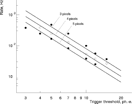
Fig. 1.: Comparison between the measured (circles) and computed trigger rates (solid lines) for different trigger settings.

Fig. 2.: Distributions of image parameters $Width$ and $Length/Size$ for the $\gamma$-rays detected from the Crab Nebula (dots with the error bars) as well as for the simulated $\gamma$-ray images (histogram).

3. Simulations

An extended library of air showers induced by primary $\gamma$-rays, protons, and nuclei was generated using a number of Monte Carlo codes available to the H.E.S.S. collaboration, ALTAI, CORSIKA, KASCADE, and MOCCA. Possible systematic uncertainties in parameters of the Cherenkov emission caused by a specific shower generator were studied in detail. Air showers were simulated within the energy range from 10 GeV to 30 TeV, and for a number of elevations in a range from 30^∘ up to the Zenith. The angle of incidence of cosmic ray showers was randomized over the solid angle around the telescope optical axis with a half opening angle of 5^∘ in order to simulate the isotropic distribution of arrival directions. Position of shower axis was uniformly randomized around the telescope over the area limited typically by a radius of 1000 m.

A procedure of simulating the camera response accounts for all efficiencies of the Cherenkov light transmission on the way from the telescope reflector to the single camera pixel. A single photo-electron response function, measured for a number of PMs, was implemented to model the PM output. Simulations trace the propagation time for each individual photon in a shower, as well as all delays related to the design of the optical reflector, PM time jitter etc. An individual photo-electron pulse shape was introduced according to the detailed time profile measured for the current electronics setup. The signal recording procedure conforms to the actual hardware design based on 1 GHz ARS ASIC with the signal integration time of 16 ns. The comparator-type trigger scheme demands a coincidence of 4 pixels in one of 38 overlapping groups of 64 pixels each but fewer near the edges of the camera. The currently used PMs trigger threshold is 140 mV, which roughly corresponds to 5 photoelectrons. The effective time window for the pixel coincidence was set to 2 ns.

4. Event Rate

The telescope trigger rate was measured for a number of pixel coincidences varying from 2 to 7, as well as for the different values of adjustable pixel trigger threshold within a range from 3 to 15 photoelectrons. A ten-minute technical run was taken for each trigger setup at an elevation about 70^∘. The simulated trigger rates reproduce the measured rates for all trigger setups with an accuracy of typically 25% (see Figure 1). For the default trigger setup (4-fold pixel coincidence with a pixel signal above 5 ph.-e.) a dead-time unfolded telescope event counting rate is about 255 Hz at an elevation of 80^∘. Given the read-out time of 1.5 ms during these early measurements it corresponds to a dead time of 40%. The Monte Carlo predicted rate is 253$\pm$18(stat)$\pm$53(syst) Hz. Air showers from cosmic ray nuclei provide about 27% of the total event rate. The muon rate represents a substantial fraction of the telescope rate. Despite the fact that muon images mimic very effectively the images from the $\gamma$-ray air showers, they offer a powerful tool for the telescope calibration using muon rings [3]. The measured and computed event rate at an elevation of 45^∘ are $\simeq 200$ Hz and 208 Hz, respectively.

5. Image Analysis

Recorded images have been cleaned using a standard two-level tail cut procedure [4]. The tail cut values were chosen as 5 and 10 ph.-e. For each image a set of second-moment parameters was calculated. Distributions of the image parameters for cosmic ray showers and for $\gamma$-ray showers extracted from the Crab Nebula data are in a good agreement with the simulations of these populations (see Figure 2). A set of optimum analysis cuts for elevation of 45^∘ is : $Alpha<\,\,9^{\circ}$; $Distance<$ 17 mrad; 0.05 mrad $<\,Width\,<$ 1.3 mrad; $Length<$ 4.8 mrad; $Length/Size<1.6\times 10^{-2}$ mrad/ph.-e.; $Size<10^{5}$ ph.-e. This set of cuts results in an acceptance for $\gamma$-ray showers at the level of 30% and cosmic ray rejection of 0.02%. It corresponds to the quality factor of about 20.

6. Performance

Applying the analysis cuts listed above to the Crab Nebula data taken mostly at an elevation of 43^∘ one can get a $\gamma$-ray rate of about $3.57\pm 0.18$ min^-1. This rate is consistent within 30% with the $\gamma$-ray rate of $2.9\pm\rm 0.18(stat)\pm 0.9(syst)$ min^-1 derived from the simulations, assuming the Crab Nebula energy spectrum as measured by HEGRA [5]. The background data rate after applying the analysis cuts is 2.5$\pm$0.1 min^-1. It is also consistent with the expectation based on the simulations, which is 2.3$\pm$0.1(stat)$\pm$0.6(syst) min^-1. The single H.E.S.S. telescope can see the signal from the Crab Nebula at the level of 9$\sigma$ after one hour of observations. A Crab-like source can be detectable at an elevation of 70^∘ after one hour of observations at the 11$\sigma$ level. The energy threshold for detected $\gamma$-rays is about 180 GeV at an elevation of 70^∘ and rises to 550 GeV at an elevation of 45^∘.

References

1. Hofmann W. 2003, these proceedings

2. Cornils R., et al. 2003, The optical system of the H.E.S.S. IACTs, Part II, accepted for publication in Astroparticle Physics

3. Leroy N., et al. 2003, these proceedings

4. Punch M. 1994, Proc. Workshop “Towards a Major Atmospheric Detector III”, Tokyo, Ed. T. Kifune, p. 163

5. Aharonian F., et al. 2000, ApJ, 539:317-324.

Chapter 6 Application of an analysis method based on a semi-analytical shower model to the first H$\cdot$E$\cdot$S$\cdot$S$\cdot$ telescope.

M. de Naurois¹, J. Guy¹, A. Djannati-Ataï² , J.-P. Tavernet¹ for the H$\cdot$E$\cdot$S$\cdot$S$\cdot$ collaboration³.
(1) LPNHE-IN2P3/CNRS Universités Paris VI & VII, Paris, France
(2) PCC-IN2P3/CNRS Collège de France Université Paris VII, France
(3) http://www.mpi-hd.mpg.de/HESS/collaboration

Abstract

The first H$\cdot$E$\cdot$S$\cdot$S$\cdot$ telescope has been in operation on-site in Namibia since June, 2002. With its fine-grain camera ($0.16^{\circ}$ pixelization) and large mirror light-collection area ($107\mathrm{m}^{2}$), it is able to see more detailed structures in the Cherenkov shower images than are characterized by the standard moment-based (Hillas) image analysis. Here we report on the application of the analysis method developed for the CAT detector (Cherenkov Array at Themis) which has been adapted for the H$\cdot$E$\cdot$S$\cdot$S$\cdot$ site and telescopes. The performance of the method as compared to the standard image analysis, in particular regarding background rejection and energy resolution, is presented. Preliminary comparisons between the predicted performance of the method based on Monte Carlo simulation and the results of the application of the method to data from the Crab Nebula are shown.

1. Introduction

In order to take advantage of the fine pixelization of the CAT camera, a new analysis method for Imaging Atmospheric Cherenkov Telescopes was developed [3]. The comparison of the shower images with a semi-analytical model was used to successfully discriminate between $\gamma$-ray and hadron-induced showers and to provide an energy measurement with a precision of the order of $20\%$, without the need for stereoscopy. The H$\cdot$E$\cdot$S$\cdot$S$\cdot$ experiment, in operation in Namibia since June 2002, combines the advantages of the different previous-generation telescopes: large mirror, fine-pixel camera and stereoscopy. In this paper, we present the improvements made to the CAT analysis in the framework of H$\cdot$E$\cdot$S$\cdot$S$\cdot$ (operating in single telescope mode).

2. Model generation

Hillas [2], studied the mean development of electromagnetic showers. We used his parametrization to construct a model of shower development, which we feed into a detector simulation to take into account instrumental effects. After this procedure, we obtain for each zenith angle $\theta$, primary energy $E$ and impact parameter $\rho$ the predicted intensity in each pixel of the camera. Model images have been generated for $30$ values between $50\,\mathrm{GeV}$ and $10\,\mathrm{TeV}$, zenith angles up to $60^{\circ}$, and impact parameters up to $300\,\mathrm{m}$ from the telescope. A multi-linear interpolation method is used to compute the pixel intensity for intermediate parameters. The model generation has been extensively tested against simulation and agrees within $10\%$ up to $10\,\mathrm{TeV}$.

3. Event reconstruction

The event reconstruction is based on a maximum likelihood method which uses all available pixels in the camera. The probability density function of observing a signal $S$, given an expected amplitude $\mu$, a fluctuation of the pedestal $\sigma_{p}$ (due to night sky background and electronics) and a fluctuation of the single photoelectron signal (p.e.) $\sigma_{s}\approx 0.4$ (PMT resolution) is given by

$$P(S|\mu,\sigma_{p},\sigma_{s})=\sum_{n=0}^{\infty}\frac{e^{-\mu}\mu^{n}}{n!\sqrt{2\pi(\sigma_{p}^{2}+n\sigma_{s}^{2})}}\exp\left(-\frac{(S-n)^{2}}{2(\sigma_{p}^{2}+n\sigma_{s}^{2})}\right)$$ (1)

The likelihood

$${\cal L}=2\sum_{\mathrm{pixel}}\log\left[P_{i}(S_{i}|\mu,\sigma_{p},\sigma_{s})\right]$$ (2)

is then maximized to obtain the primary energy, the target direction $T$ and the impact point $I$. This five parameter fit can be reduced to four parameters $E$, $\rho$, $\phi$ (azimuthal angle in the camera) and $d$ (angular distance of the shower barycenter to the primary direction, see fig. 1), using the alignement of the image centre of gravity with $\mathrm{TI}$.

Fig. 1.: Definition of geometrical parameters used for the shower reconstruction. O is the center of the camera, G the image barycenter and T the reconstructed target direction.

4. Signal extraction

The following cuts are used in signal extraction

• A cut on the ratio of the shower length $L$ to its amplitude $S$, designed to reject small muon images : $L/S\leq 1.6\times 10^{-2}\mathrm{mrad}\ \mathrm{p.e.}^{-1}$

• A geometrical cut of the distance mismatch $\left|\delta D\right|\leq 5\ \mathrm{mrad}$, where $\delta D=\left|\mathrm{TG}\right|-\left|\mathrm{OG}\right|$. This cut selects $\gamma$-rays originating from the center of the field of view and is orthogonal to the commonly used $\alpha$ orientation angle.

• A goodness of fit ${\cal G}<0.07$ defined from the likelihood distribution as function of the number of operating pixels $N_{\mathrm{dof}}$ as ${\cal G}=(\left<{\cal L}\right>-{\cal L})/N_{\mathrm{dof}}$, where the average likelihood and its RMS are obtained by integration of an analytical approximation of eq. 1:

  $$\left<{\cal L}\right>=-\sum_{\mathrm{pixel}}\left(1+\log 2\pi+\log\left(\mu(1+\sigma_{s}^{2})+\sigma_{p}^{2}\right)\right),\quad\sigma_{\cal L}^{2}=2$$ (3)

The distribution of $\cal G$ for simulated $\gamma$-rays and real hadrons is shown in fig. 2 together with the likelihood’s average and RMS. The distribution for $\gamma$-rays is compatible with an expected mean of $0.0$ and has a slightly larger RMS than the expected value $\sqrt{2/N_{\mathrm{dof}}}\approx 5\times 10^{-2}$. A cut ${\cal G}\leq 0.07$ keeps $77\%$ of the $\gamma$-rays and rejects $82\%$ of the hadrons.

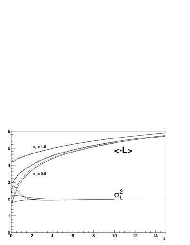
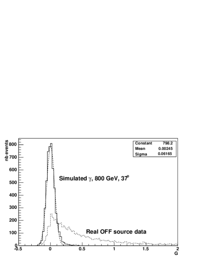
Fig. 2.: Left: Likelihood curves for different night sky backgrounds. Solid curves are numerical integrations, dashed curves are simple analytical approximations (eq. 3). Right: Goodness of fit ($\cal G$) distribution after $L/S$ and $D$ cuts, for simulated $\gamma$ and real OFF source events.

5. Results

We have analysed $20$ pairs on the Crab Nebula, corresponding to $4.65$ hours (live-time corrected) of data. Fig. $3$ shows the comparison between the standard H$\cdot$E$\cdot$S$\cdot$S$\cdot$ analysis [4] and this work. The model analysis alone produces an $\alpha$ plot extending up to $180^{\circ}$. The significance in the $\alpha<9^{\circ}$ is better in the hillas analysis ($21\,\sigma$ against $16.9\,\sigma$), mainly because the hadron rejection is not yet fully optimized for the model analysis, but the $\alpha$ resolution is much better in the Model analysis ($2.7^{\circ}$ against $4.2^{\circ}$), thus providing a better signal to background ratio in the first bins.

More interesting is the background rejection capability of a combined analysis. The lower plot of fig. 3 shows the $\alpha$ distribution of the events passing both the Hillas and Model analysis cuts. The signal over background ratio is increased by a factor of more than $3$, reaching the value of $4.8$ for $\alpha<9^{\circ}$ wheras less than $15\%$ of the $\gamma$-rays are lost. This also results in a net increase in significance up to $25.2\,\sigma$. The complementarity of the hadron rejection capabilities of both analyses is a very powerful instrument for finding faint sources, and was successfully used to detect the blazar PKS 2155-304 in October 2002 at the level of $7.4\,\sigma$ [1].

This analysis also provides energy and shower impact measurements with respective resolutions of about $20\%$ and $20\ \mathrm{m}$ at $800\,\mathrm{GeV}$.

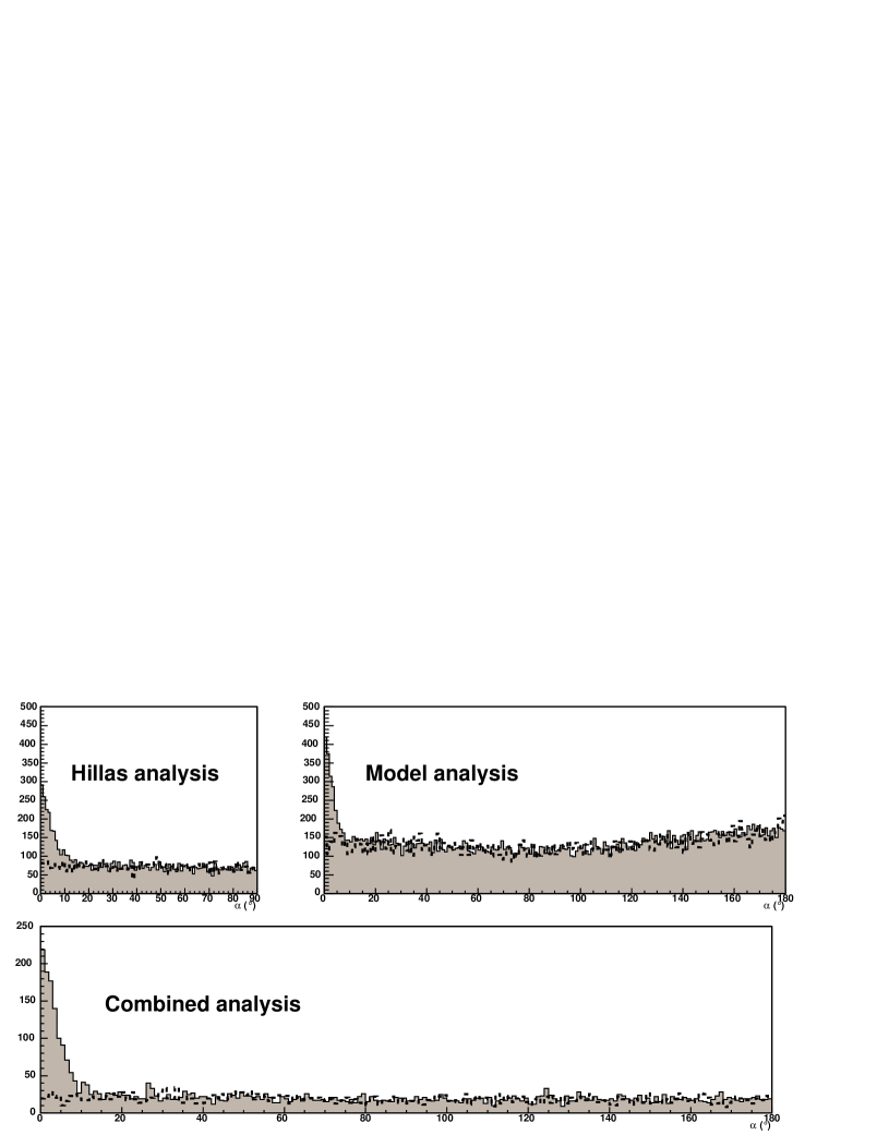
Fig. 3.: Results of the model analysis. Solid lines: ON source. Dashed lines: OFF source. top left: $\alpha$ plot with standard H$\cdot$E$\cdot$S$\cdot$S$\cdot$ analysis based on hillas parameters. top right: Corresponding $\alpha$ plot for the model analysis. bottom: Effect of the combination of the cuts on the background.

6. Conclusion

We have developed a powerful analysis for H$\cdot$E$\cdot$S$\cdot$S$\cdot$ based on the comparison of shower images with a semi-analytical model. This analysis provides a better $\alpha$ angle measurement than the standard analysis (base on Hillas parameters), as well as good energy and shower impact resolution. Moreover, the combination of both analysis provides an additional background rejection factor of about $3$, which leads to an important increase in significance. This combination method has been successfully used to detect the blazar PKS 2155-304 at the level of respectively $13\,\sigma$ and $7.4\,\sigma$ in July and October 2002. Further results will be presented at the conference.

7. References

1. Djannati-AtaïA, These proceedings

2. Hillas A.M.. 1982, J. Phys. G 8, 1461

3. Le Bohec S et al., NIM A416 (1998) 425

4. Masterson C, These proceedings

Chapter 7 The Central Data Acquisition System of the H.E.S.S. Telescope System

C. Borgmeier¹, N. Komin¹, M. de Naurois², S. Schlenker¹, U. Schwanke¹ and C. Stegmann¹, for the H.E.S.S. collaboration
(1) Humboldt University Berlin, Department of Physics, Newtonstr. 15, D-12489 Berlin, Germany
(2) Laboratoire de Physique Nucleaire et des Hautes Energies, 4 place Jussieu, T33 RdC, 75252 Paris Cedex 05, France

Abstract

This paper gives an overview of the central data acquisition (DAQ) system of the H.E.S.S. experiment. The emphasis is put on the chosen software technologies and the implementation as a distributed system of communicating objects. The DAQ software is general enough for application to similar experiments.

1. Introduction

The High Energy Stereoscopic System (H.E.S.S.) is an array of imaging Čerenkov telescopes dedicated to the study of non-thermal phenomena in the Universe. The experiment is located in the Khomas Highlands of Namibia. At the end of Phase I, the array will consist of four telescopes, two of which are already operational and being used for data-taking at the time of writing.

Each telescope in the array is a heterogeneous system with several subsystems that must be controlled and read out. The telescope subsystems comprise a camera with 960 individual photo-multiplier tubes, light pulser systems for calibration purposes, a source tracking system, an IR radiometer for atmosphere monitoring, and a CCD system for pointing corrections. Common to the whole array is a set of devices for the monitoring of atmospheric conditions, including a weather station, a ceilometer and an all-sky radiometer.

2. DAQ System Requirements

The DAQ system provides the connectivity and readout of all the systems mentioned above. It takes over run control, the recording of event and slow control data, error handling, and monitoring of all subsystems. The remoteness and small bandwidth connection of the H.E.S.S. site imply that the DAQ system must be stable and easily operated.

The main data stream is produced by the cameras which generate events with a size of 1.5 kB. At the design trigger rate of 1 kHz, this yields a maximum data rate of 6 MB/s for four telescopes, resulting in roughly 100 GB of data per observation night. The data rates from the other subsystems are significantly smaller.

On the hardware side the requirements are met by a Linux PC farm with a fast Ethernet network. The details are described in [1].

3. DAQ Software

The H.E.S.S. DAQ system is designed as a network of distributed C++ and Python objects, living in approximately 100 multi-threaded processes for the H.E.S.S. Phase I configuration.

For inter-process communication the omniORB [2] implementation of the CORBA protocol standard is used which provides language bindings for C++ and Python. CORBA allows to call methods of objects in remote processes and to pass data objects. The transport and storage of objects needs a serialization mechanism which is provided by the ROOT Data Analysis Framework [3]. Both the ROOT-based H.E.S.S. data format and the ROOT graphics and histogram classes are used online and offline allowing a seamless integration of data analysis code and hence fast feedback.

The base classes for all DAQ applications are provided by a central library. Derived classes, implementing the base class interfaces, control for example a hardware component or handle different types of data streams. Each DAQ process contains a StateController object which implements inter-process communication and run control state transitions.

The DAQ system distinguishes four different process categories as shown in Fig. 1. The Controllers directly interact with the hardware and read out the data. Each hardware component is controlled by one Controller process. The Controllers push the data to intermediate Receivers, which perform further processing and store the data. The Receivers also provide an interface that allows other processes to sample processed data. Readers actively request data from the Receivers at a rate different from the actual data-taking rate. The data or derived quantities are then available for display and monitoring purposes. Manager processes are not involved in the data transport but control the data-taking.

Fig. 1.: Types of processes in the DAQ system

4. DAQ Configuration

Different data-taking configurations of the array correspond to different run types. A run type is defined by a set of required Controllers, Receivers, Readers, and Managers. Examples for run types are the observation run type with all available subsystems, various calibration run types for the cameras, and dedicated run types for testing and data-taking with specific subsystems, e.g. the tracking system. An actual run is given by its type and a set of parameters.

All run type definitions, run parameters, the configuration of the DAQ system, and observation schedules are stored in a MySQL database acting as central information source and logging facility for the DAQ system.

Setting up the required processes for a specific run type is simplified by combining related processes in groups that are called contexts. An example for a context is CT1 which comprises all Controllers accessing the hardware of telescope number 1. Every context contains one Manager that controls the other processes in the context. At startup, the Manager reads the processes in its context from database tables and launches them. The Manager serves as an intervention point to all processes in the context, passes on state transitions, and takes over error handling in predefined ways.

For data-taking a central DAQ Manager reads the observation schedule from the database and determines the actual sequence of runs according to the availability of contexts. Runs that require different contexts can be processed in parallel. The central DAQ Manager launches the required context Managers and initiates the run preparation. After the preparation of a run the starting and stopping of the data-taking is taken over by a dedicated Manager which controls the participating contexts.

The shift crew interacts with the DAQ system via a central control GUI providing an access point to the system and direct monitoring of the states of the different processes (cf. Fig. 2 (left)). Data monitoring information is shown by a variety of different displays. The displays are generated by instances of a generic Reader which are configurable via database tables allowing a simple and flexible setup of the quantities to be displayed. Fig. 2 (right) shows some examples of monitoring displays.

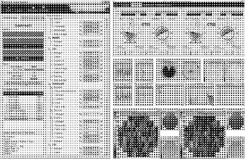
Fig. 2.: Central control GUI (left) and examples of monitoring displays (right)

5. Summary and Outlook

The described system is in operation since the start of the observation program with the first telescope. The setup based on database tables proved its flexibility when integrating new subsystems into the data-taking. Processing parallel runs was exercised in the commissioning phase when observing with the first telescope while aligning the mirrors of the second telescope. The system is now taking data with two telescopes and is expected to scale well to the full Phase I array.

Acknowledgments. This work was supported by the Bundesministerium für Bildung und Forschung under the contract number 05 CH2KHA/1.

6. References

1. Borgmeier C. et al. 2001, Proceedings of ICRC 2001: 2896

2. S.L. Lo and S. Pope, The Implementation of a High Performance ORB over Multiple Network Transports, Distributed Systems Engineering Journal, 1998.
See also http://omniorb.sourceforge.net

3. R. Brun and F. Rademakers, ROOT – An Object Oriented Data Analysis Framework, Proceedings AIHENP’96 Workshop, Lausanne, Sep. 1996, Nucl. Inst. & Meth. in Phys. Res. A 389 (1997) 81–86.
See also http://root.cern.ch

Chapter 8 Mirror alignment and performance of the optical system of the H.E.S.S. imaging atmospheric Cherenkov telescopes

René Cornils,¹ Stefan Gillessen,² Ira Jung,² Werner Hofmann,²
and Götz Heinzelmann,¹ for the H.E.S.S. collaboration
(1) Universität Hamburg, Institut für Experimentalphysik, Luruper Chaussee 149, D-22761 Hamburg, Germany
(2) Max-Planck-Institut für Kernphysik, P.O. Box 103980, D-69029 Heidelberg, Germany

Abstract

The alignment of the mirror facets of the H.E.S.S. imaging atmospheric Cherenkov telescopes is performed by a fully automated alignment system using stars imaged onto the lid of the PMT camera. The mirror facets are mounted onto supports which are equipped with two motor-driven actuators while optical feedback is provided by a CCD camera viewing the lid. The alignment procedure, implying the automatic analysis of CCD images and control of the mirror alignment actuators, has been proven to work reliably. On-axis, 80% of the reflected light is contained in a circle of less than 1mrad diameter, well within specifications.

1. Introduction

H.E.S.S. is a stereoscopic system of large imaging atmospheric Cherenkov telescopes currently under construction in the Khomas Highland of Namibia [5]. The first two telescopes are already in operation while the complete phase 1 setup, consisting of four identical telescopes, is expected to start operation early 2004. The reflector of each telescope consists of 380 mirror facets with 60 cm diameter and a total area of 107 $\mathrm{m}^{2}$. For optimum imaging qualities, the alignment of the mirror facets is crucial. A fully automated alignment system has been developed, including motorized mirror supports, compact dedicated control electronics, various algorithms and software tools [1-3]. The specification for the performance of the complete reflector requires the resulting point spread function to be well below the size of a pixel of the Cherenkov camera.

2. Mirror alignment technique

The adjustable mirror unit consists of a support triangle carrying one fixed mirror support point and two motor-driven actuators. A motor unit includes the drive motor, two Hall sensors shifted by $90^{\circ}$ sensing the motor revolutions and providing four TTL signals per turn, and a 55:1 worm gear. The motor is directly coupled to a 12 mm threaded bolt, driving the actuator shaft by 0.75 mm per revolution. One count of the Hall sensor corresponds to a step size of 3.4 $\mu$m, or 0.013 mrad tilt of the mirror. The total range of an actuator is about 28 mm which corresponds to 6.15^∘ tilt of the mirror facet.

The alignment uses the image of an appropriate star on the closed lid of the PMT camera. The required optical feedback is provided by a CCD camera at the center of the dish, which is viewing the lid as illustrated in Fig. 1 (left). Individual mirror facets are adjusted such that all star images are combined into a single spot at the center of the PMT camera. The basic algorithm is as follows: a CCD image of the camera lid is taken. The two actuators of a mirror facet are then moved one by one, changing the location of the corresponding spot on the lid. These displacements are recorded by the CCD camera and provide all information required to subsequently position the spot at the center of the main focus. This procedure is repeated for all mirror facets in sequence.

It is – to our knowledge – the first time that such a technique is used to align the mirrors of Cherenkov telescopes. The major advantages of this approach are evident: a natural point-like source at infinite distance is directly imaged in the focal plane, and the alignment can be performed at the optimum elevation.

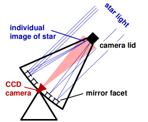
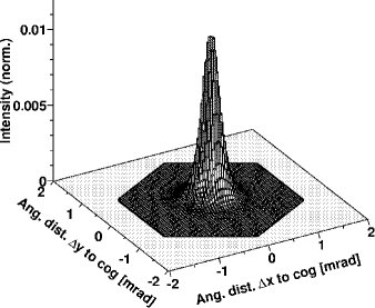
Fig. 1.: Left: Mirror alignment technique. The telescope is pointed towards an appropriate star whereupon all mirror facets generate individual images of this star in the focal plane. Actuator movements change the location of the corresponding image which is observed by a CCD camera. Right: On-axis intensity distribution of a star on the camera lid after alignment. The hexagonal border indicates the size of a pixel of the PMT camera defined by the shape of the Winston cones.

3. Point spread function

Fig. 1 (right) shows a CCD image of the image of a star on the camera lid after the alignment of all mirror facets in relation to the size of a PMT pixel (0.16^∘ diameter). The intensity distribution represents the on-axis point spread function for telescope elevations within the range used for the alignment (55^∘–75^∘). The distribution is symmetrical without pronounced substructure and the width of the spot is well below the PMT pixel size.

To parameterize the width of the intensity distributions, different quantities are used: the rms width $\sigma_{proj}$ of the projected (1-dimensional) distributions and the radius $r_{80\%}$ of a circle around the center of gravity of the image, containing 80% of the total intensity. On the optical axis, the point spread function is characterized by the values $\sigma_{proj}=0.23$ mrad and $r_{80\%}=0.41$ mrad (requirements: $\leq$0.5 and $\leq$0.9 mrad, respectively). This is an excellent result.

3.1. Variation of the point spread function across the field of view

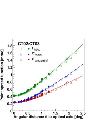
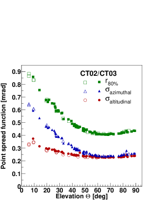
Fig. 2.: Point spread function of the first two operational H.E.S.S. telescopes (CT03 and CT02). Left: Width of the point spread function as a function of the angular distance $\theta$ to the optical axis at elevations around $65^{\circ}$. Right: Width of the point spread function as a function of telescope elevation $\Theta$.

Optical aberrations are significant in Cherenkov telescopes due to their single-mirror design without corrective elements and their modest $f/d$ ratios. At some distance from the optical axis, the width of the point spread function is therefore expected to grow linearly with the angle $\theta$ to the optical axis. For elevation angles around $65^{\circ}$, where the mirror facets were aligned, Fig. 2 (left) summarizes the spot parameters as a function of the angle $\theta$. Besides $r_{80\%}$, the rms widths of the distributions projected on the radial ($\sigma_{radial}$) and tangential ($\sigma_{tangential}$) directions are given. The measurements demonstrate that the spot width primarily depends on $\theta$; no other systematic trend has been found and the width $r_{80\%}$ is well described by

$$r_{80\%}=(0.42^{2}+0.71^{2}\theta^{2})^{{}^{1}/_{2}}\quad[\textrm{mrad}].$$ (1)

To verify that the measured intensity distribution is quantitatively understood, Monte Carlo simulations of the actual optical system were performed, including the exact locations of all mirrors, shadowing by camera masts, the measured average spot size of the mirror facets, and the simulated precision of the alignment algorithm. The results are included in Fig. 2 (left) as solid lines, and are in good agreement with the measurements:

$$r_{80\%}=(0.42^{2}+0.72^{2}\theta^{2})^{{}^{1}/_{2}}\quad[\textrm{mrad}].$$ (2)

3.2. Variation of the point spread function with telescope pointing

At fixed elevation, no significant dependence of the point spread function on telescope azimuth was observed. In contrast, a variation with elevation is expected due to gravity-induced deformations of the telescope structure. Fig. 2 (right) illustrates how the spot widths $r_{80\%}$, $\sigma_{azimuthal}$, and $\sigma_{altitudinal}$ change with elevation $\Theta$. The width $r_{80\%}$ is to a good approximation described by

$$r_{80\%}=(0.41^{2}+0.96^{2}(\sin\Theta-\sin 66^{\circ})^{2})^{{}^{1}/_{2}}\quad[\textrm{mrad}].$$ (3)

For elevations most relevant for observations, i.e. above $45^{\circ}$, the spot size $r_{80\%}$ varies by less than 10%. At $30^{\circ}$ it is about 40% larger than the minimum size but still well below the size of the PMT pixels. A detailed analysis of the deformation of the support structure [2,4] revealed that the stiffness is slightly better than initially expected from finite element simulations.

4. Conclusion

The mirror alignment of the first two H.E.S.S. telescopes was a proof of concept and a test of all technologies involved: mechanics, electronics, software, algorithms, and the alignment technique itself. All components work as expected and the resulting point spread function significantly exceeds the specifications. Both reflectors behave almost identical which demontrates the high accuracy of the support structure and the reproducibility of the alignment process.

References

1. Bernlöhr K., Carrol O., Cornils R., Elfahem S. et al. 2003, The optical system of the H.E.S.S. imaging atmospheric Cherenkov telescopes, Part I, accepted

2. Cornils R., Gillessen S., Jung I., Hofmann W. et al. 2003, The optical system of the H.E.S.S. imaging atmospheric Cherenkov telescopes, Part II, accepted

3. Cornils R., Jung I. 2001, Proc. of the 27th Int. Cosmic Ray Conf., eds. Simon M., Lorenz E., and Pohl M. (Copernicus Gesellschaft), vol. 7, p2879

4. Cornils R., Gillessen S., Jung I., Hofmann W., Heinzelmann G. 2002, to appear in The Universe Viewed in Gamma-Rays, (Universal Academy Press)

5. Hofmann W. 2003, these proceedings

Chapter 9 Calibration results for the first two H$\cdot$E$\cdot$S$\cdot$S$\cdot$ array telescopes.

N.Leroy,¹ O.Bolz,² J.Guy,³ I.Jung.,² I.Redondo,¹ L.Rolland,³ J.-P.Tavernet,³ K.-M.Aye,⁴ P.Berghaus,⁵ K.Bernlöhr,² P.M.Chadwick,⁴ V.Chitnis,³ M.de Naurois,³ A.Djannati-Ataï,⁵ P.Espigat,⁵ G.Hermann,² J.Hinton,² B.Khelifi,² A.Kohnle,² R.Le Gallou,⁴ C.Masterson,² S.Pita,⁵ T.Saitoh,² C.Théoret,⁵ P.Vincent³ for the H$\cdot$E$\cdot$S$\cdot$S$\cdot$ collaboration⁶.
(1) LLR-IN2P3/CNRS Ecole Polytechnique, Palaiseau, France
(2) Max Planck Institut für Kernphysik, Heidelberg, Germany
(3) LPNHE-IN2P3/CNRS Universités Paris VI & VII, Paris, France
(4) Department of Physics, University of Durham, Durham, United Kingdom
(5) PCC-IN2P3/CNRS College de France Université Paris VII, Paris, France
(6) http://www.mpi-hd.mpg.de/HESS/collaboration

Abstract

The first two telescopes of the H$\cdot$E$\cdot$S$\cdot$S$\cdot$ stereoscopic system have been installed in Namibia and have been operating since June 2002 and February 2003 respectively. Each camera [2] is equipped with 960 PMs with two amplification channels per pixel, yielding both a large dynamic range up to 1600 photo-electrons and low electronic noise to get high resolution on single photo-electron signals. Several parallel methods have been developed to determine and monitor the various calibration parameters using LED systems, laser and Cherenkov events. Results including pedestals, gains, flat-fielding and night sky background estimations will be presented, emphasizing the use of muon images for absolute calibration of the camera and mirror global efficiency, including lower atmosphere effects. These methods allow a precise monitoring of the telescopes and have shown consistent results and a very good stability of the system since the start of operation.

1. Introduction

The H$\cdot$E$\cdot$S$\cdot$S$\cdot$ detector performance can be monitored with calibration data obtained each night of Cherenkov observation. Methods of calibration and monitoring using LED and laser systems, and also Cherenkov events from muon rings and arcs are presented here.

2. “Classical” calibration

At the initial calibration step, the ADC to photo-electron($\gamma$e) coefficient (ADC$\gamma$e) is determined using an LED system providing a $\sim 1\gamma$e pulsed signal; the $\gamma$e distribution follows a Poisson distribution with an average value of $1\gamma$e. The single $\gamma$e spectrum is described by a sum of Gaussian functions normalized by the Poisson probability to have from 1 to $n$ $\gamma$e; the pedestal being represented by a Gaussian function weighted by the probability of having zero $\gamma$e (fig. 1(a)). The gain of every pixel is monitered showing good stability apart from those PMs whose base has been damaged by a bright illumination (see figure 1(b)).

The relative pixel efficiencies are measured using a laser located at the centre of the mirror which provides a uniform illumination in the focal plane. The ADC$\gamma$e are then flat-fielded with these relative efficiencies. To acquire information on electronic noise (typically $0.18\gamma$e) some data are also taken with the lid closed and the high voltages on. Such runs provide baseline parameters to take into account temperature dependencies in the electronics response, for example the pedestal position is shifted by 10 ADC counts/${}^{\circ}\mathrm{C}$.

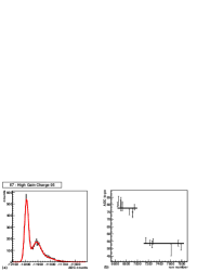
Fig. 1.: (a) Example of gain determination in high gain channel. (b) Gain of one damaged pixel with run number; the gain decrease is due to a too bright illumination.

Finally, some calibration parameters are determined for each Cherenkov run. First the pedestal position is determined every minute of acquisition to take account the above-mentionned temperature dependance. Then the Night Sky Background (NSB) value for each pixel is determined by using the HVI (High Voltage Intensity) shift or the pedestal charge distribution. HVI represents the sum of the anode and divider currents; a baseline value is determined in the runs with closed lid.

In addition, the pixels to be excluded from the analysis are identified, for example those with a star in the field of view, with high voltage switched off or unstable. Also ARS readout chips [2] (each serving 4 channels) with incorrect read-out settings are searched for. After the detector commissioning, the mean number of pixels excluded from the analysis is $\sim$ 40 (4%).

3. Calibration with muon rings

Another useful tool for the calibration of Cherenkov telescopes is provided by muons produced in hadronic showers which cross the mirror, whose Cherenkov light is emitted at low altitude (up to 600m above each H$\cdot$E$\cdot$S$\cdot$S$\cdot$ telescope). The intensity of the muon images can be used to measure the absolute global light collection efficiency of the telescope.

(a)

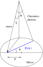
(b)

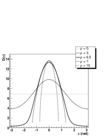
Fig. 2.: (a) Geometry of the Cherenkov emission from a muon near the mirror: $\xi$ is the inclination of the muon to the vertical, $\rho$ the impact parameter, and $\theta$ the Cherenkov angle. (b) $D(\phi)$ for different impact parameters.

The two principal advantages of using muons are : 1) an easily modelled Cherenkov signal is used, and 2) the calibration includes all detector elements in the propagation. For a muon impacting the telescope, the number of $\gamma e$ detected in the camera can be expressed [1] as

$$\frac{\mathrm{d}N}{\mathrm{d}\phi}=\epsilon\frac{\alpha I}{2}\sin(2\theta)D(\phi)$$ (1)

where $I$ is the integrated photon wavelength, $\epsilon$ the average collection efficiency, $\theta$ the Cherenkov angle of the muon, $\alpha$ the fine structure constant, $\phi$ the azimuthal angle of the pixel in the camera and $D(\phi)$ is a geometrical factor representing the length of the chord defined by the intersection between the mirror surface (assumed circular and ignoring gaps between mirror tiles) and the plane defined by the muon track and the Cherenkov photon (see figure 2 (a) and (b)).

(a)

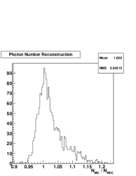
(b)

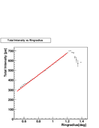
Fig. 3.: (a) Distribution of the ratio between MC photons and reconstructed photons with the muon analysis. (b) Total intensity vs. Cherenkov angle on Crab data. The solid line is the dependance in radius from eqn. 1.

The Cherenkov emission modelling includes the geometry of the ring (centre position, radius, width), impact parameter, and light collection efficiency. These parameters are determined by a $\chi^{2}$ minimization.

This method has been tested by simulating muons falling near the telescope. Figure 3(a) shows that the number of photons generated from the MC simulation is well reconstructed by the muon analysis. Thus, muon data can be very useful to test the simulation of the H$\cdot$E$\cdot$S$\cdot$S$\cdot$ instrument. The model is also able to provide a good reconstruction of real data. In figure 3(b) the solid line shows the expected dependance with $\theta$ (muon ring radius) from eqn. 1. The data points beyond radius 1.2 are due to a small number of misreconstructed rings (4% of the muon events).

Figure 4(a) shows the evolution of the collection efficiency for Cherenkov photons between 200 and 700 nm for observation runs from complete rings ($\sim$1 Hz). The variations are less than 10% and it is possible to see the effects of hardware changes. No significant correlations with zenith and azimuth angles are observed.

The presence of a large number of muon arcs ($\sim\mathrm{10\,Hz}$) in every data run allows us to determine the light collection efficiency of each individual pixel relatively to the rest of the camera on a run-by-run basis. The relative efficiencies are determined from the mean of the residuals between data and the model fit in each pixel. The residuals follow a Gaussian distribution with small tails due to bad or incorrectly calibrated pixels. The RMS of these efficiencies is $\sim 7$%, consistent with laser measurements. This method, which also includes incomplete rings in order to increase the available statistics, provides a very sensitive monitoring tool. The figure 4(b) shows the monitoring of two PMs, the damaged channel was overexposed to light.

(a)

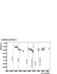
(b)

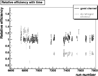
Fig. 4.: (a) Collection efficiency of Cherenkov light from muon analysis with time. Some hardware changes are indicated. The run numbers are from October to December 2002. (b) Monitoring of the relative efficiencies of two channels.

4. Conclusion

The calibration methods used by the H$\cdot$E$\cdot$S$\cdot$S$\cdot$ experiment utilize LED and laser systems dedicated to this purpose and also Cherenkov images from local muons selected from the collected data. These independent methods allow us to monitor detector response on the few percent level, and additionally provide information for the selection of runs of good quality.

5. References

1. Vacanti G. et al  1994, Astroparticle Physics 2, 1

2. Vincent P. et al  2003, These proceedings

Chapter 10 Arcsecond Level Pointing Of The H.E.S.S. Telescopes

Stefan Gillessen¹ for the H.E.S.S. collaboration²
(1) MPI für Kernphysik, P.O. Box 103980, D-69029 Heidelberg, Germany
(2) http://www.mpi-hd.mpg.de/HESS/collaboration

Abstract

Gamma-ray experiments using the imaging atmospheric Cherenkov technique have a relatively modest angular resolution of typically 0.05 to 0.1 degrees per event. The centroid of a point-source emitter, however, can be determined with much higher precision, down to a few arcseconds for strong sources. The localization of the Crab TeV source with HEGRA, for example, was dominated by systematic uncertainties in telescope pointing at the 25 arcsecond level. For H.E.S.S. with its increased sensitivity it is therefore desirable to lower the systematic pointing error by a factor of 10 compared to HEGRA. As the exposure times are on a nanosecond scale it is not necessary to actively control the telescope pointing to the desired accuracy, as one can correct the pointing offline. We demonstrate that we can achieve the desired 3 arcseconds pointing precision in the analysis chain by a two step procedure: a detailed mechanical pointing model is used to predict pointing deviations, and a fine correction is derived using stars observed in a guide telescope equipped with a CCD chip.

1. Introduction

Each H.E.S.S. telescope has a stiff support structure that bears the alt/az-mounted primary mirror and the camera in the primary focus. In combination with the drive system the construction allows the detector to point with an accuracy of $\sim$60 arcseconds to any position in the sky. However, the centroid of TeV point sources can be determined to an accuracy of few arcseconds. Thus the systematic pointing error should be lowered to the same level.

Aside from an improved instrumental sensitivity this also has astrophysical applications. M87 [1] is one example, where arcsecond level pointing allows for the determination of whether the TeV-emission is coming from the centre of the galaxy or from the jet, as the separation is $\sim$10 arcseconds. A high pointing resolution can also contribute to the distinction between pulsar and nebula emission for plerionic sources hosting a pulsar. In addition a possible future TeV detection of the galactic centre requires the localization of the emission to a few arcseconds.

2. Methods and Limits

Due to mechanical imperfections of a telescope, its pointing is not fully determined by the axes’ positions. There are pointing errors due to:

• Reproducible mechanical errors, e.g. the bending of the structure under gravity or imperfectly aligned axes

• Irreproducible effects, such as wind loads or obstacles on the drive rails

Reproducible errors can be determined once, then predicted and corrected in the future. Irreproducible effects can only be corrected by the observation of some known reference - preferably star light. In H.E.S.S. the approach is to predict reproducible errors ($1^{st}$ step) and then employ a fine correction based on the observation of stars in parallel to TeV observations ($2^{nd}$ step). Unfortunately the camera (basically a phototube array) cannot be used to determine the correction as the point spread function of the dish is comparable in size with the pixels of the array [2].

Therefore a CCD camera is mounted on the dish. It observes the images of stars on the closed lid of the camera [2]. The such recorded positions in the focal plane are related to the phototubes using LEDs mounted in the corners of the array. By observing many bright stars, the mispointing as a function of altitude and azimuth is sampled. Afterwards a detailed mechanical model, whose parameters describe the reproducible mechanical errors, is fit to the data. It allows in turn the first step correction: Given a telescope pointing the model returns the expected mispointing. A nice side-effect is, that the mechanical meaning of the fit parameters can be used to monitor the mechanical stability of the telescopes.

The fine correction is determined using a guide telescope mounted parallel to the optical axis. It registers stars with a second CCD camera (“SkyCCD”). After identification using a pattern match algorithm the stars’ positions are predicted using a similar mechanical model, but with different offsets and focal length. The observed positions will differ from the prediction due to the mispointing (including irreproducible effects and reproducible errors not represented by the model). Thus the difference measures the mispointing and it is therefore the fine correction to be applied.

Table 1.: Limits of the Pointing Asccuracy

Principle Limits	Measured Values	Sum
Accuracy of the reference LED positions	1.4”
Reproducibility of the mechanical deformations	1.4”
Stability of the tracking system	1.3 ”
Accuracy of star position determination	0.8 ”	2.5”
Limits for Mechanical Model
Positioning accuracy of the drive system	3.5”
Deformations of the drive rails’ shapes	3.5”
Principle limits (above)	2.5”
Inaccuracy of the shaft encoders	2 x 1.5”	5.9”

Table 1 lists the effects that limit the pointing accuracy when using these methods and shows their respective contributions as measured. The mechanical model should achieve a pointing resolution of $\sim$6 arcseconds (2D rms). Using the fine correction should further improve it to 2.5 arcseconds.

3. Results

The pointing of the first two telescopes has been studied. As the results are similar only data for the first telescope is presented. An example of measured mispointing vectors as a function of altitude and azimuth is given in Fig. 1. Without any correction the raw mechanical pointing accuracy is 28 arseconds (2D rms) as Fig. 2 shows. After application of the model, the residual is 8 arcseconds, approximately in agreement with the limit for the mechanical model (Table 1).

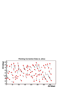
Fig. 1.: Measured mispointing for the first telescope as a function of altitude and azimuth. Arrows are artificially enlarged

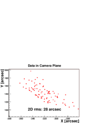
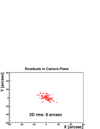
Fig. 2.: Left: Raw positions in the focal plane before the application of the model
Right: After application of the fit (same scale)

In order to test the fine correction, the SkyCCD has recorded the same stars that are used for the determination of the mechanical model. The same kind of model is used to describe these positions in the SkyCCD, resulting in similar residuals. If the residuals in the focal plane are actually due to mispointing, they must agree point by point with the residuals from the SkyCCD fit. A correlation plot for two residuals is given in Fig. 3, clearly showing the expected correlation. Thus the SkyCCD residual can be used to measure the focal plane residual, allowing for the desired fine correction. After its application a 2D rms of $\sim$2.5 arcseconds remains, which agrees with the principle limit from Table 1.

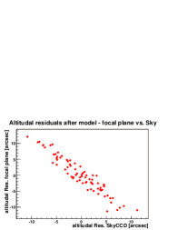
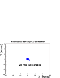
Fig. 3.: Left: (Vertical) residual in the focal plane vs. residual in SkyCCD
Right: Positions in the focal plane after the fine correction (same scale as Fig. 1)

4. Conclusion

The described two-step procedure allows the offline pointing control of the H.E.S.S. telescopes to attain the desired accuracy of 2.5 arcseconds. It will allow H.E.S.S. to address many morphological questions in TeV astronomy.

1. F.A. Aharonian et al. (HEGRA collaboration)  2003, A&A 403, L1-L5

2. R. Cornils et al.   2003, The optical system of the H.E.S.S. imaging atmospheric Cherenkov telescopes, Part II, submitted to APP

Chapter 11 A Novel Alternative to UV-Lasers Used in Flat-fielding VHE $\gamma$-ray Telescopes

K.-M. Aye,¹ P.M. Chadwick,¹ C. Hadjichristidis,¹ I.J. Latham,¹ R. Le Gallou,¹
A. Noutsos,¹ T.J.L. McComb,¹ J. McKenny,¹ J.L. Osborne,¹ S.M. Rayner¹
for the H.E.S.S. collaboration
and J.E. McMillan.²
(1) Department of Physics, Rochester Building, Science Laboratories, University of Durham, Durham, DH1 3LE, UK
(2) Department of Physics and Astronomy, University of Sheffield, Sheffield, S3 7RH, UK

Abstract

Preliminary tests of an alternative calibration system for the H.E.S.S. telescope array show that it is possible to replace the currently operating UV-Laser device with an optical LED apparatus. Together with complementary optics, it is able to simulate the Cherenkov flashes, while at the same time illuminating the whole of the telescope’s camera uniformly. The device in question is capable of driving a fixed number of specifically chosen LEDs to produce frequent flashes of very short duration similar to the Cherenkov emission generated by electromagnetic cascades. The design of the system continues to be refined. We describe the components and the operation of the device as developed so far.

1. Introduction

Calibration and monitoring of H.E.S.S. cameras is crucial for the post-processing of the recorded events. Exact knowledge of the individual gain for each photomultiplier tube (PMT) is required to translate the number of photoelectrons (p.e.) produced by the PMTs into the air shower’s energy. This information can be acquired by using a well defined light source situated on the telescope, simulating Cherenkov flashes, and by recording the output from the camera’s PMTs. One can summarise what specifications this light source should have to optimally match Cherenkov flashes. Chiefly, the light source’s flashes should be as short as a few ns and have a spectrum that, ideally, matches that of the Cherenkov flash (see Fig. 1). Furthermore, it will have to be wide enough so as to cover the camera completely. Last but not least, its light beam should be uniform so that each PMT receives the same amount of reference light during a flash.

The flat-fielding device used with the first H.E.S.S. telescope was based on a UV-LASER which would, in conjunction with a scintillator, produce short ($<$7 ns), frequent pulses [1]. Whilst this system performs well, there are several disadvantages, notably cost, a relatively low repetition rate, the problems inherent in the use of optical fibres and poor long-term stability. We therefore wanted to improve the device for later H.E.S.S. telescopes.

While keeping our initial requirements for such a device within acceptable standards, we have constructed a much cheaper (6 times less), much higher repetition rate (40 times more) and much easier to maintain flat-fielding system.

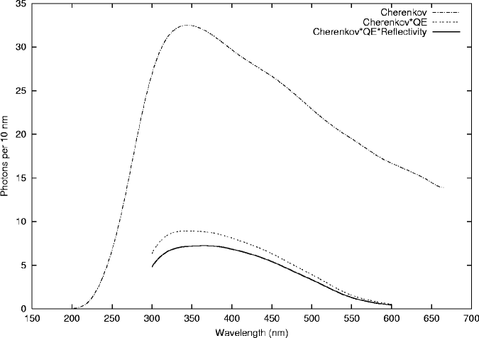
Fig. 1.: The Cherenkov Spectrum for 1 TeV $\gamma$-rays at the Gamsberg plateau in Namibia (H.E.S.S. site). The dash-dotted line is derived from MOCCA simulations. The dotted line represents the same spectrum with the PMT’s quantum efficiency (QE) included. The solid line is the simulated spectrum with both the PMT’s QE and the mirror’s reflectivity taken into account.

2. The System

2.1. General Description - Circuitry

The flat-fielding device is composed of two independent circuits; the main circuit, which produces the actual flashes, and a monitoring sub-circuit, which monitors the light output coming from the LEDs. A complete schematic of the device is shown in Fig. 2.

The main circuit is triggered via an RS232 interface controlled by the H.E.S.S. central data acquisition system via a W&T Com-Server. The RS232 pulses are fed at the speed of 19600 bauds into an RS232-to-TTL converter that converts them to TTL gates. The UV-LASER system could only be triggered as fast as 25 Hz due to limitations of the laser itself. Our new system uses a trigger rate of 1 kHz, making it a useful tool for testing the response of the DAQ system under high incident event rates.

Apart from the remote operation of the device, a built-in switch allows us to feed in TTL pulses from a local pulse generator (TTL-in mode). When set to the opposite position, the switch sends the TTL signature to an external display, thus allowing the monitoring of the remote operation (TTL-out mode).

The TTL signal, either coming from a remote or a local source, is directed into a driver, which is responsible for transforming the former into a signal compatible with the pulser circuits. These pulser circuits have been built by Sheffield University for the Antares collaboration, for timing calibration purposes [3]. There are 3 of these pulsers connected in parallel in the current configuration, all conveniently embedded on one board and each carrying a single LED. In front of the LED/pulser array there are a filterwheel, a monitoring photodiode, a diffuser and a UV-transparent window (Fig. 2).

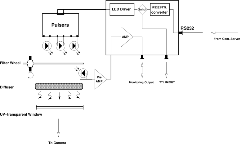
Fig. 2.: The layout of the flat-fielding device.

2.2. System components

The ‘heart’ of the flat-fielding system is the LED pulser developed by Sheffield University. A complete description of the device can be found in [2]. It exhibits low jitter ($<$0.5 ns) and a pulse drift rate $<$0.25 ns/y [3]. Our tests confirmed that this pulser produces pulses with a FWHM of $\simeq$5 ns and a rise time of about 2.5 ns, a significant improvement from the UV-LASER system, whose pulse rise time is 3.3 ns [1]. We also found that the pulse intensities deviate by less than 5% RMS.

Most of the LEDs we tested were found to be compatible with the Sheffield pulser. The current configuration at the H.E.S.S. site uses the HUVL400-520 LEDs by HERO Electronics. Their spectrum ranges from 390 to 410 nm and their half-intensity angle is 20^∘.

The response of a PMT varies with intensity and the calibration process should take into account these gain variations to result in more accurate flat-fielding. Hence, an automated filter wheel is installed in front of the LEDs to control the intensity of the light output. It is supplied by Elliot Scientific and is capable of holding 6 filters. Currently, it holds 5 neutral density filters —supplied by Coherent-Ealing—, graded as follows: 0.5, 1.0, 1.3, 1.5 and 2.0; while one position is left empty to transmit the full intensity. By analysing the data recorded during the calibration runs, we can estimate the number of p.e. that the H.E.S.S. PMTs detected from the flat-fielding apparatus. Using the filter wheel settings we can get a photon flux per pulse ranging from 2.5 to 250 ph cm^-2 at a distance of 15 m.

A complementary accessory that allows the monitoring of the LED intensity without having to access the dish is also part of the flat-fielding system. It is based on a photodiode and allows us to monitor the light pulses with, e.g. an oscilloscope.

Since it is crucial to have the same photon intensity on all of the PMTs when calibrating them, it was decided to place a diffuser before the UV-window in the flat-fielding apparatus. We used a 25 mm diameter holographic diffuser by Coherent-Ealing that produces a circular diffusing output $20^{\circ}$ wide, for collimated incident light beams.

In order to protect the flat-fielding apparatus from the weather, we shielded it with a UV-transparent window made of borosilicate glass supplied by Edmund Optics. The window’s transmissivity, in the frequency range between 350 and 800 nm, is $\approx$90%.

3. References

1. Chadwick, P.M. et al. 2001, Flat-fielding of H.E.S.S. phase I, Proc. 27th Int. Cosmic Ray Conf., 2919

2. McMillan, J.E. 2001, Using the Sheffield Pulser, private communication

3. McMillan, J.E. on behalf of the ANTARES Collaboration  2001, Calibration Systems for the ANTARES Neutrino Telescope, Proc. 27th Int. Cosmic Ray Conf., 2919

Chapter 12 Atmospheric Monitoring For The H.E.S.S. Project

K.-M. Aye, P.M. Chadwick, C. Hadjichristidis, M.K. Daniel¹, I.J. Latham, R. Le Gallou, J.C. Mansfield, T.J.L. McComb, J.M. McKenny, A. Noutsos, K.J. Orford, J.L. Osborne, and S.M. Rayner for the H.E.S.S. Collaboration
Dept. of Physics, University of Durham, DH1 3LE Durham, United Kingdom
(1) now at Department of Physics and Astronomy, Iowa State University, Ames, IA 50011-3160, USA.

Abstract

Several atmospheric monitoring devices have been installed at the H.E.S.S. site in Namibia. Firstly, Heitronics KT19 infrared radiometers, aligned paraxially with the H.E.S.S. telescopes, measure the infrared radiation of the water in clouds crossing the telescope field of view. Correlations between the trigger rate of the telescope and these IR measurements are shown in this paper. For a general judgment of the atmosphere’s transmittance, i.e. the detection of any light-attenuating aerosols, a ceilometer – a LIDAR with built-in atmospheric data reduction code – is being used. The overall status of the weather is monitored by a fully automated weatherstation.

1. Overview

The main causes of extinction of Cherenkov light are absorption and Rayleigh scattering by molecules, and Mie scattering by aerosols. The H.E.S.S. photomultipliers and mirrors are sensitive to light between 250 and 700 nm. In this range the only light-absorbing molecule is ozone, but the most significant loss of Cherenkov light in the case of a ‘clear’ sky is caused by Rayleigh scattering off all atmospheric molecules dominant at lower wavelengths due to its $\lambda^{-4}$ dependance, and Mie scattering on aerosols which becomes dominant above approximately 400 nm [2].

2. Weatherstation

A UK Meteorogical Office approved weatherstation from Campbell Scientific has been installed at the H.E.S.S. site. It records air temperature, relative humidity, atmospheric pressure, wind speed, wind direction and rainfall 24 hours a day. The data acquisition (DAQ) is integrated in the standard DAQ scheme for the camera data and therefore allows efficient cross-checking of atmospheric conditions and camera data. The weather data are especially important for providing input values for atmospheric models constructed with the commercially available MODTRAN package in connection with radiometer and LIDAR (“LIght Detection And Ranging”) data.

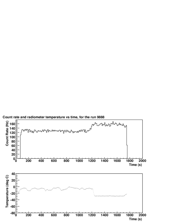
Fig. 1.: Correlation between telescope count rate and radiometer temperature due to Cherenkov light absorption by cloud.

3. The Ceilometer

A Vaisala CT25K Ceilometer has been installed at the site. A Ceilometer is a LIDAR with cloud detection and ranging facility and built in algorithms to invert the received light power to backscatter values in units of $\mathrm{(km\cdot sr)^{-1}}$. Using an InGaAs diode laser working at $(905\pm 5)$nm, the Ceilometer detects backscatter mainly due to aerosol scattering out to 7.5 km. The backscatter profile can be inverted to recreate the optical density profile for the atmosphere. This profile can be compared to profiles from model atmospheres which then can be used to calculate the extinction in the wavelength range of interest, i.e. 250 to 700 nm. Results of preliminary studies can be found in a parallel paper [1].

Fig. 2.: The relation between sky temperature and elevation angle of the radiometer with different winow materials. Ambient conditions in Namibia: nighttime, $T=16^{\circ}C$, rel.Humidity 41%; Durham: afternoon, $T=5^{\circ}C$, rel. Humidity $(70\pm 10)\%$

4. Infrared radiometer

The Heitronics KT19.82A Mark II is a radiometer designed for measuring the infrared radiation in the transmission window between 8 and 14$\mathrm{\mu}$m [4]. We use it to measure the infrared radiation from the sky in its field of view of 2.9^∘. By comparing the observed quantity to a blackbody spectrum, the radiometer then calculates the ‘radiative’ temperature of the sky. It has been shown [3] that the measured sky temperature is very sensitive to the presence of clouds and water vapour which is crucial for determining the cause of a variation in the count rate of an IACT. Although clouds are not significantly warmer than the surrounding atmosphere, they are more effective emitters of blackbody radiation than the atmosphere in this wavelength range. If there are no clouds, the temperature still can vary from night to night due to relative humidity and temperature changes which may induce ice crystallisation on aerosols and therefore change the scattering phase function of Mie scattering.

Two of the planned four telescopes of H.E.S.S Phase 1 are presently operational and on each of them a radiometer is installed paraxially to provide an immediate means of cloud detection in the field of view of the camera. Figure 1 shows the detection of the clearance of the sky after a period of high cloud. Furthermore a scanning radiometer is installed to give the shift crew an immediate overview of the sky for any presence of clouds or approaching weather fronts.

In addition to detecting clouds, the radiometer data can be used to determine the amount of water vapour contained in the atmosphere, a quantity on which the transmissivity of the latter for Cherenkov light depends. Such a measurement is not trivial. The temperature measured by the radiometer depends on several parameters: the temperature and water vapour profile of the atmosphere, the observing zenith angle, and the material of the window used to protect the instrument from the weather. Semi-empirical models like the one from Idso [5] try to relate the infrared flux detected by the radiometer to the temperature and the water vapour pressure measured at ground level in a quantitative way. Indeed, we have measured such a correlation in our data, but nevertheless this model is not satisfactory and a suitable one has yet to be found.

4.1. Zenith angle and window material dependencies

The temperature measured with the radiometer for a clear sky increases with the zenith angle due to a thicker section of the warm atmosphere being sampled [3]. In figure 2 one can see the zenith angle dependence for different window materials in front of the radiometer lens. This window protects the lens of the radiometer from weather, but as it emits in the infrared, its influence on the measured value of the radiometer is quite significant, depending on the chosen material. As one can see it not only increases the measured temperatures, but also alters the sensitivity ($T(\theta_{max})-T(\theta_{min})$). For this reason, the thin polyethylene film, whilst less robust than Cleartran™, is the chosen material for the protective window.

Moreover, the parametrization of the zenith angle dependence of the radiometer measurement can provide a differential estimate of the water vapour content of the atmosphere, which can in turn be related to its profile.

5. Conclusion

To conclude, we can say that the atmospheric monitoring instruments for the HESS experiment are now installed and running. Their observations have yet to be understood in some details and exploited to a fuller degree in order to let them allow us to estimate the actual transmissivity of the atmosphere to Cherenkov light to a better extent than so far.

6. References

1. Aye et.al., Implications of LIDAR observations at the H.E.S.S. site in Namibia for energy calibration of the atmospheric Cherenkov telescopes, this conference

2. Bernlohr K. 2000, Astroparticle Physics 12, 255-268

3. Buckley et.al. 1999, Experimental Astronomy 9, p237-249

4. http://www.heitronics.de,  Accessed 2003-05-13

5. Idso S.B. 1981, Water Resources Research 17, p295-304

Chapter 13 Implications of LIDAR Observations at the H.E.S.S. Site in Namibia for Energy Calibration of the Atmospheric Cherenkov Telescopes

K.-M. Aye, P.M. Chadwick, C. Hadjichristidis, M.K. Daniel¹, I.J. Latham, R. Le Gallou, T.J.L. McComb, J.M. McKenny, S.J. Nolan², A. Noutsos, K.J. Orford, J.L. Osborne, and S.M. Rayner for the H.E.S.S. Collaboration
Dept. of Physics, University of Durham, DH1 3LE Durham, United Kingdom
¹ now at Iowa State University USA. ² now at Purdue University USA

Abstract

Scattering values returned by a LIDAR installed at the H.E.S.S. site may be used for calculating optical depth profiles. One may then construct model atmospheres which fit these using the commercially available MODTRAN atmospheric radiation transfer code. Examples of the results of Monte Carlo simulations of the telescope response for two characteristic atmospheres are shown.

1. Introduction

As an instrument for ground-based astronomy the atmospheric Cherenkov telescope (ACT) is unusual in that the atmosphere is an integral part of the detection system. Its stucture, essentially the pressure-altitude profile, controls the particle shower development and the Cherenkov emission. The atmospheric attenuation, as a function of altitude and wavelength, determines the probability of the Cherenkov photons reaching the ACT. Monitoring the properties of the atmosphere is therefore essential for the interpretation of the Cherenkov signal in terms of the energy spectrum of the gamma-rays and source flux variation. The atmospheric attenuation in the 250 to 700 nm range depends on molecular absorption, Rayleigh scattering and Mie scattering by aerosols [1]. Mie scattering is expected to be the most time-variable component. We describe a LIDAR instrument which gives information on this for 7.5 km above the ACT. The generation of model atmospheres to fit the LIDAR measurements is still in development but an example of the differences in ACT response for two characteristic atmospheres is given in the final section.

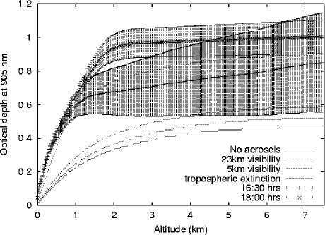
Fig. 1.: Optical depth generated by the ceilometer backscatter data (the 2 graphs with large error bars) and calculated by MODTRAN for different visibilities

2. The Ceilometer

The Vaisala CT25K Ceilometer is a commercial LIDAR (LIght Detection And Ranging) which measures cloud heights and vertical visibilities by sending out light pulses at $(905\pm 10)$nm with a pulsed InGaAs diode laser. As the laser pulse traverses the sky, the resulting backscatter profile signal strength over height is stored and processed with a sampling interval of 100 ns, resulting in a spatial resolution of 30m.

The general description of the instantaneous return signal strength is given as the LIDAR equation

$$P_{r}(z)=E_{0}\frac{c}{2}\frac{A}{z^{2}}\beta(z)e^{-2\tau(z)}$$ (1)

where $P_{r}(z)$ is the instantaneous power received from distance $z$, $E_{0}$ the effective pulse energy in Joules (taking all optical attenuation into account, measured by internal monitoring), $c$ the speed of light, $A$ the receiver aperture (in m²sr), $\beta(z)$ the volume backscatter coefficient at distance $z$ (in m^-1sr^-1) and $\tau(z)=\int_{0}^{z}\alpha(z^{\prime})dz^{\prime}$ the optical depth (OD) at $z$ produced by an attenuation coefficient $\alpha(z)$, the factor 2 accounting for the travel out and back.

2.1. The Backscatter Coefficient

The volume backscatter coefficient $\beta(z)$ is a result of combined molecular (Rayleigh) and aerosol (Mie) scattering. Although the attenuation $\alpha(z)$ is unknown, it can be assumed to correlate the backscatter with the attenuation via the Lidar Ratio $k$: $\beta(z)=k\alpha(z)$ [3]. The Lidar Ratio can take values between 0.02 in high humidities to 0.05 in low humidities, but is mostly assumed to be 0.03 [2]. Figure 1 shows OD profiles which have been generated from the backscatter data by summing the backscatter values over the sampled time-bins like $\tau(z)=\sum_{z}\frac{\beta(z)}{k}$. Also plotted are model OD profiles generated by MODTRAN 4 [4] for a default tropical atmosphere with differing aerosol profiles ranging from a minimal OD for no aerosols included (solid line) to a rural profile with 5 km visibility (dashed line inside the errors of the lower ceilometer profile).

Fig. 2 Shows preliminary OD profiles generated from backscatter data taken under clear sky conditions for 2 different values of the lidar ratio $k$ (0.05 and 0.02 respectively). These curves lie beneath the minimum curve for the OD resulting only from Rayleigh scattering and molecular absorption of Fig. 1 (no aerosols). This is because the ceilometer’s internal algorithm’s primary purpose is to identify significant backscatter from cloud layers. Distances between 100 and 900 m from the receiver have the optimum signal to noise for determining this and when no significant scatter is detected the machine automatically sets scatter to zero in this region. This drawback can be compensated for with the modelling done with the MODTRAN package, this is ongoing work and results are expected to be shown on the conference poster accompanying this paper. Once out of the optimum signal to noise range the algorithm once again starts to give non-zero, albeit noisy, values. Starlight extinction measurements and the observation of a calibrated light source on a distant hill will help resolve uncertainties in the backscatter coefficient.

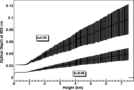
Fig. 2.: Optical densities created from ceilometer backscatter data on a very clear night for 2 different values of the lidar ratio

3. Monte Carlo Simulations

Radio sonde measurements at Windhoek show that the annual mean atmospheric pressure profile is close to the MODTRAN ‘tropical’ model. Monte Carlo simulations using the MOCCA shower code and an adaptation of the CAMERAHESS ACT simulation code show that the seasonal variation from this model have a significantly smaller effect on the ACT response than likely variations in the atmospheric attenuation. The current standard atmospheric attenuation model for Monte Carlo simulations of H.E.S.S. ACT response is a maritime haze aerosol model from 0 to 2 km above sea level, a tropospheric spring-summer model for 2 to 10 km and a layer of default stratospheric dust. This is referred to as Atm.8 in figure 3. The zenith angle is typical of that for observations of the Crab nebula. The site, being at an altitude of 1.8 km, is above most of the model’s maritime haze as was the the HEGRA site on the island of La Palma, for which the model was chosen. As H.E.S.S. is on a plateau more than 100 km from the sea this model could be regarded as being among the lower of the levels of attenuation likely to be encountered. A straightforward variant of this model is Atm.11 which puts the base of the 2 km of maritime haze at 1.8 km. Both have the ‘tropical’ structure. The reduction in effective area for triggering is shown in figure 3.

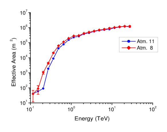
Fig. 3.: The effective area of a single H.E.S.S. ACT for triggering by gamma-rays incident at $50^{\circ}$ zenith angle for two characteristic aerosol profiles.

4. References

1. Bernlöhr K. 2000, Astropart. Phys. 12, 255

2. Filipcic A., Horvat M., Veberic D., Zavrtanik D., Zavrtanik M. 2003, Astropart.Phys. 18, 501-512

3. Klett J.D. 1981, Appl. Optics 20, 211; 1985, ibid 24, 1638

4. MODTRAN patented US software, US Air Force Phillips Laboratories

Chapter 14 Optical Observations of the Crab Pulsar using the first H.E.S.S. Cherenkov Telescope

A. Franzen,¹ S.Gillessen,¹ G.Hermann,¹ and J. Hinton¹
for the H.E.S.S. Collaboration
(1) Max-Planck-Institut für Kernphysik, PO Box 103980, D-69029 Heidelberg, Germany

Abstract

For the understanding of the mechanisms of particle acceleration in pulsars, it is necessary to determine the high energy cutoff of the pulsed emission. In order to derive upper limits (or detections) on the pulsed emission in the TeV energy range using Cherenkov telescopes, typically data taken over periods of months or even years are superimposed. It is therefore necessary to use a time capture system and analysis tools which provide a base for pulsar phase analysis which is stable over a time-scale of years. We have built a device consisting of a photomultiplier tube with a fast current digitization system and components of the timing system of the H.E.S.S. experiment, which allows to measure pulsed optical emission making use of the large mirror area of Cherenkov telescopes. The system was installed into the first H.E.S.S. Cherenkov telescope in January 2003, where data was taken over 8 nights on the Crab and Vela pulsars. Optical pulsation from the Crab pulsar could be measured with observation times as short as a second. This system can therefore be used to determine the pulsar phase and to monitor the short term and long term stability of the timing system of the H.E.S.S. experiment.

1. Introduction

The new generation of ground based gamma-ray experiments currently under construction will provide improved sensitivity and thresholds in the sub-100 GeV region. One of the science goals of these experiments (H.E.S.S., MAGIC, CANGAROO, VERITAS) is to investigate the upper energy range for pulsed emission from EGRET pulsars.

Detections or upper limits on pulsed emission will likely involve the combination of data taken over months and even years. It is therefore necessary to prove the long term stability of the timing systems used by these experiments and also the proper performance of the analysis software. It should also be noted that contemporary ephemerides are not always available and that many of the pulsars of interest suffer frequent glitches. There is, therefore, a clear motivation for regular optical monitoring of pulsars by gamma-ray observatories.

The goal of the experiment described here was to develop and demonstrate an apparatus for fast timing measurement of optical signals to be used for monitoring the timing system of the H.E.S.S. experiment. Previous optical fast timing measurements are described in [1,2].

2. Experimental Method

The H.E.S.S. Experiment is an array of four Cherenkov telescopes with 15 m focal length and 107 m² mirror area, located in Namibia ($23^{\circ}16^{\prime}$ S, $16^{\circ}30^{\prime}$ E, at 1800 m). The optical properties of the H.E.S.S. telescopes are described in [3].

The experiment described here utilized the first complete H.E.S.S. telescope and a custom-built detector installed on the closed lid of the Cherenkov camera. A silver coated plane mirror mounted at $45^{\circ}$ to the telescope axis was used to place a lid-mounted photomultiplier tube (PMT) in the centre of the focal plane of the primary mirror. An aperture stop limited the field of view of the PMT to 23 mm (equivalent to $5^{\prime}$), matched conservatively to the point-spread-function (PSF) of the telescope. The average spectral sensitivity (quantum efficiency $\times$ reflectivity of primary and secondary mirrors) in the 300-600 nm range was 0.11.

The PMT (Photonis XP2960 with passive base) signal was read out via a shaping amplifier (FWHM of response 100$\,{\mu}$s) and digitized using a 16-bit ADC, sampling at 20 kHz. Each sample is accompanied by a timestamp derived from a GPS clock (Meinberg 167, precision $<1\,\mu$s) via a custom-built VME counter module. The anode signal was DC coupled in order to easily measure background light levels as well as pulsation. See Figure 1 for details.

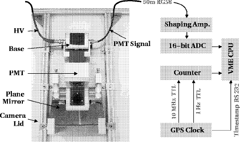
Fig. 1.: Mechanical and electronic setup of the experiment.

3. Measurements

To achieve the required tracking precision of $\sim 1^{\prime}$ it was necessary to make online corrections for atmospheric refraction and bending in the arms of the telescope. To verify the absolute pointing of the instrument, several offset pointing runs and drift scans were made of bright stars (with an 0.01 neutral density filter in place). These runs verified that $>80$% of the light in the PSF was collected onto the PMT. Observation runs were made in a cycle of HV off (to monitor the ADC pedestal position) and on-source runs. Several empty fields were also observed as background references. The typical PMT anode current was 2-6 ${\mu}$A depending on the region observed.

After removing data compromised by unstable weather conditions, 6 hours of data on the Crab (spread over 8 nights from the 21- 29 January) remain. 10 hours of data were obtained on the Vela pulsar.

4. Results and Discussion

The first step of the analysis is to barycentre the time associated with each sample using the standard H.E.S.S. software scheme. The barycentred time is then folded using radio ephemerides from the Jodrell Bank Observatory [4] (with frequency and first derivative from 15.1.03 and second derivative from the period 12.02-2.03). After a phase position is established, 4 consecutive samples are summed to provide independent current measurements for the light-curve. The data are then split into 10-second slices, each of which is tested for stability by examining the RMS of the DC signal. Figure 2 shows the phasogram extracted from a single 10 second slice. The expected double-peaked structure is clearly visible on top of a large DC background.

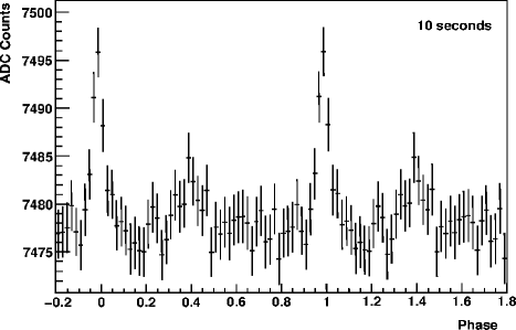
Fig. 2.: Optical  signal from the Crab pulsar from a 10 second observation

The sum of slices passing the RMS cut (with the DC component subtracted) is shown in Figure 3. The position, width, and relative heights of the two peaks are consistent with the measurement made by the Hubble Space Telescope [1]. The significance of the pulsation is $\approx 4\sigma/\sqrt{t/\mathrm{seconds}}$. Each complete phase contains $\approx 800$ photoelectrons, seen against a background of $\approx 2\times 10^{6}$ pe. The phase position of the mean peak can be determined with a precision of $30\,\mu$s in $\sim$30 minutes and is stable over the period of observations (see Figure 4 right).

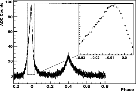
Fig. 3.: Left: the Crab pulsar phasogram extracted from the full data-set of 3 hours of best quality observations. Right: The position of the main peak as a function of time during the measurement. The mean position of $-0.0061\pm 0.0004$ is consistent with the result of $-0.0058$ given by [2].

Observations of the Vela pulsar were also made during this period, however, with the 10 hours obtained, no significant pulsation was observed (using ephemerides from [5]). We estimate $\sim 30$ hours would be required for a $5\sigma$ detection with this instrument.

5. Outlook

This prototype device has demonstrated the utility of an optical monitoring device for high energy gamma-ray experiments. We are currently developing an improved device with multiple light sensors (for the exclusion of optical transients, for example meteorites) and possibly higher quantum efficiency light sensors. A search for optical Giant Pulses in our data-set is under way.

We would like to thank our technical support staff in Namibia, T. Hanke, E. Tjingaete and M. Kandjii, for their excellent support and D. Lewis for providing ephemerides for the Vela pulsar.

6. References

1. Percival J. W. et al. 1993, ApJ 407, 276

2. Straubmeier C. et al. 2001, Exp. Astron. 11, 157

3. Cornils R.  et al. 2003, Submitted to Astropart. Phys.

4. Jodrell Bank pulsar group page, http://www.jb.man.ac.uk/$\sim$pulsar/

5. Lewis, D. (University of Tasmania), private communication.