A Dynamical Systems Approach to an Inviscid and Thin Accretion Disc

Abstract

The inviscid and thin accretion disc is a simple and well understood model system in accretion studies. In this work, modelling such a disc like a dynamical system, we analyse the nature of the fixed points of the stationary solutions of the flow. We show that of the two fixed points, one is a saddle and the other is a centre type point. We then demonstrate, using a simple but analogous mathematical model, that a temporal evolution of the flow is a very likely non-perturbative mechanism for the selection of an inflow solution that passes through the saddle type critical point.

Keywords : Dynamical systems, Transonic flows, Accretion discs

1 Introduction

In astrophysical fluid dynamics, studies in accretion processes occupy a position of prominence. Of such processes, critical (transonic) flows — flows which are regular through a critical point — are of great importance [1]. A classic example of such a flow, in the stationary spherically symmetric situation, is the Bondi flow [2]. What is striking about the Bondi solution is that while it is virtually impossible to numerically generate it in the stationary limit of the hydrodynamic flow, it is easy to lock on to the Bondi solution when the temporal evolution of the flow is followed. This dynamic and non-perturbative selection mechanism of the transonic solution is in very favourable agreement with Bondi’s conjecture that it is the criterion of minimum energy that will make the transonic solution the favoured one [2, 3].

The appeal of the spherically symmetric flow, however, is somewhat pedagogic, limited as it is by its not accounting for the fact that in a reasonably realistic situation, the infalling matter would be in possession of angular momentum — and hence the process of infall should lead to the formation of what is known as an accretion disc. A well understood and quite regularly invoked model of such a system is the inviscid and thin accretion disc [1, 4, 5, 6]. In this work, we show how such a physical system — studied in its stationary limit — gives rise to saddle point like behaviour for at least one of the critical points of the flow. The adverse implications regarding the realizability of a solution passing through such a point is then addressed by considering the system in a real non-linear time evolution. A simplified mathematical analog of such a situation shows that the evolution indeed selects the critical (transonic) solution. Finally, we discuss that in the vicinity of the critical point, the resulting perturbation equation arising out of a linear stability analysis of the stationary solutions, quite closely resembles the metric of an acoustic black hole, and that is probably the signal that trajectories pass through the critical point in a unidirectional fashion.

2 The stationary equations of the flow and its critical points

The flow system to be considered is an axisymmetric thin disc of a compressible astrophysical fluid, with a thickness $H$ [7]. In the vertical direction the flow is considered to be in hydrostatic equilibrium. The governing equations for the flow should therefore be the equation of continuity and the equations for momentum balance in both the radial and the azimuthal directions. It is customary to write the stationary flow equations in the following notation [8].

• Equation of continuity:

  $$\frac{d}{dR}(\rho RHv)=0$$ (1)

• Radial momentum balance equation:

  $$v{\frac{dv}{dR}}+{\frac{1}{\rho}}{\frac{dP}{dR}}+\left({{{\Omega}_{K}}^{2}}-{{\Omega}^{2}}\right)R=0$$ (2)

• Angular momentum balance equation:

  $$v{\frac{d}{dR}}(\Omega R^{2})={\frac{1}{\rho RH}}{\frac{d}{dR}}\left({\frac{\alpha\rho{c_{s}}^{2}R^{3}H}{{\Omega}_{K}}}{\frac{d\Omega}{dR}}\right)$$ (3)

In the above, $v$ is the radial velocity, $R$ is the radial distance, $\Omega$ is the angular velocity, ${\Omega}_{K}$ is the Keplarian angular velocity defined as ${{\Omega}_{K}}^{2}=GM/R^{3}$, $c_{s}$ is the velocity of sound defined as ${c_{s}}^{2}={\partial}P/{\partial}{\rho}$ and $\alpha$ is the effective viscosity of Shakura and Sunyaev [9].

It is a standard practice to make use of a general polytropic equation of state $P=k{\rho}^{\gamma}$ where $k$ and $\gamma$ are constants, with $\gamma$ being the polytropic exponent [10], whose admissible range $(1<\gamma<5/3)$ is restricted by the isothermal limit and the adiabatic limit respectively. The condition of hydrostatic equilibrium along a direction perpendicular to the thin disc, allows for the use of the approximation $(H/R){\cong}({c_{s}}/{v_{K}})$, where ${v_{K}}=R{\Omega}_{K}$  [7]. In that case Eq. (1) leads to

$${c_{s}}^{2n+1}vR^{5/2}={\rm constant}$$ (4)

where $n=(\gamma-1)^{-1}$. Combining Eqs. (2) and  (4) yields,

$${\frac{d}{dR}}(v^{2})={\frac{2v^{2}}{R}}\left[{\frac{5{c_{s}}^{2}/(\gamma+1)-({{\Omega}_{K}}^{2}-{\Omega}^{2})R^{2}}{v^{2}-2{c_{s}}^{2}/(\gamma+1)}}\right]$$ (5)

and a first integral of Eq. (3) can be written as

$${\alpha}\frac{d}{dR}({\Omega}^{2})=2{\Omega}\left(\Omega-{\frac{L}{R^{2}}}\right){\frac{v{\Omega}_{K}}{{c_{s}}^{2}}}$$ (6)

where $L$ is a constant of integration.

We now consider the inviscid limit of Eq. (6) by setting $\alpha=0$. This, somewhat simplifying, prescription has found regular favour in accretion literature [4, 5, 6], and it gives the condition ${\Omega}R^{2}=L$, where $L$, which can be physically identified as the specific angular momentum of the flow, now becomes a constant of the motion. Such a constraint allows us to fix the critical points of the flow. At such points both the numerator and the denominator in the right hand side of Eq. (5) vanish simultaneously [1, 6], and this will deliver the critical point conditions as

$${v_{c}}^{2} = {\frac{2{c_{sc}}^{2}}{\gamma+1}}$$

$${\frac{5{c_{sc}}^{2}}{\gamma+1}} = ({{\Omega}_{Kc}}^{2}-{{\Omega}_{c}}^{2}){R_{c}}^{2}$$ (7)

with the subscripted label $c$ indicating critical (fixed) point values. We should be able to find $v_{c}$ and $R_{c}$ from Eqs. (7). The second relation above, which is actually a quadratic in $R_{c}$, leads us to

$$R_{c}=\frac{\gamma+1}{10}\frac{GM}{{c_{{sc}}}^{2}}\left[1\pm\sqrt{1-\frac{20}{\gamma+1}\left(\frac{c_{{sc}}L}{GM}\right)^{2}}\right]$$ (8)

and this gives the two critical points at radii $R=R_{c1}$ and $R=R_{c2}$, with ${R_{c2}}>{R_{c1}}$. To fix the critical point coordinates $(R_{c},v_{c})$, we need to look at the integral of Eq. (2), which reads as

$${\frac{v^{2}}{2}}+{\frac{L^{2}}{2R^{2}}}-{\frac{GM}{R}}+{\frac{{c_{s}}^{2}}{\gamma-1}}={\rm constant}={\frac{{{c_{s}}^{2}}(\infty)}{\gamma-1}}$$ (9)

in which the constant of integration has been determined with the help of the boundary condition that for very great radial distances, the speed of sound approaches a constant “ambient” value $c_{s}(\infty)$, while $v\longrightarrow 0$. In this expression we use the condition ${v_{c}}^{2}=2{{c_{sc}}^{2}}/(\gamma+1)$ and the value of $R_{c}$ from Eq. (8), to fix $c_{sc}$ in terms of the constants of the system. This will in turn fix the critical point coordinates $(R_{c},v_{c})$.

3 The disc as a dynamical system

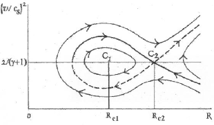
Figure 1: A schematic diagram of the accretion problem. The fixed point $\rm{C_{2}}$ is a saddle point. $\rm{C_{1}}$ is a centre type point. The separatrices pass through $\rm{C_{2}}$.

To have any understanding of the nature of the critical points of the inviscid and thin disc being studied here, we need to cast the equation giving the stationary solutions of the disc system, along the lines of a dynamical system. To do that we appeal to Eq. (5) and parametrize it in the form

$${\frac{d\left(v^{2}\right)}{d\tau}} = 2v^{2}\left[{\frac{5{c_{s}}^{2}}{\gamma+1}}-\left({{\Omega}_{K}}^{2}-{\Omega}^{2}\right)R^{2}\right]$$

$${\frac{dR}{d\tau}} = R\left[v^{2}-{\frac{2{c_{s}}^{2}}{\gamma+1}}\right]$$ (10)

It is to be noted that the parametrization has been carried out in an arbitrary mathematical parameter space $\tau$, and in such a space the two equations above represent a dynamical system. To analyse the nature of the fixed points, we expand and linearize about the fixed point coordinates $({v_{c}}^{2},R_{c})$ in Eqs. (10), and in terms of the perturbed quantities we obtain a set of linear equations given by

$${\frac{d}{d\tau}}\left({\delta}v^{2}\right) = 2{v_{c}}^{2}\left[-{\frac{5}{2}}{\frac{\gamma-1}{\gamma+1}}{\delta}v^{2}+\left({\frac{6-4{\gamma}}{\gamma+1}}{\frac{GM}{{R_{c}}^{2}}}-{\frac{L^{2}}{{R_{c}}^{3}}}{\frac{7-3{\gamma}}{\gamma+1}}\right){\delta}R\right]$$

$${\frac{d}{d\tau}}\left({\delta}R\right) = {R_{c}}\left[{\frac{2\gamma}{\gamma+1}}{\delta}v^{2}+5{\frac{\gamma-1}{\gamma+1}}{v_{c}}^{2}{\delta}R\right]$$ (11)

Use of solutions of the form $e^{\lambda\tau}$ would deliver the eigenvalues $\lambda$ — growth rates of ${\delta}v^{2}$ and ${\delta}R$ — as

$${\lambda}^{2}=4{\frac{\left(5-\gamma\right)}{\left(\gamma+1\right)^{2}}}\frac{GM}{R_{c}}{c_{sc}}^{2}\left[\beta-{\frac{L^{2}}{{L_{Kc}}^{2}}}\right]$$ (12)

where $\beta=(5-3{\gamma})/(5-{\gamma})$ and the local Keplerian angular momentum is $L_{Kc}=\sqrt{GMR_{c}}$. It is now quite evident that if $R_{c}$ is the outer fixed point $R_{c2}$, then ${\lambda}^{2}$ is positive and the fixed point is saddle type, while if $R_{c}$ is the inner point $R_{c1}$, then ${\lambda}^{2}$ is negative and the fixed point is centre type. We show the trajectories in Fig.1, in which the arrows indicate the direction of flows.

The fixed point $\rm{C_{2}}$ at $R=R_{c2}$ is the saddle. In a manner of speaking, it may be dubbed the “sonic point” because one of the two trajectories passing through it is transonic, rising from subsonic values far from it to supersonic values when $R<R_{c2}$. This trajectory is shown as the heavy solid curve, and is the accretion flow. The heavy dashed curve is the wind. The above demonstration that the fixed point $\rm{C_{2}}$ is a saddle has adverse implications regarding the realizability of the transonic trajectory passing through it. Conventional wisdom about the nature of saddle type points [11] gives us to believe that if we go directly to the static limit of the dynamic evolution, then the transonic trajectory would not be realizable. However, it is generally believed that transonic trajectories do occur in astrophysical systems such as the one being studied here [1]. Our contention is that it is the temporal evolution of such a system that selects the transonic trajectory. This selection mechanism is purely non-perturbative as opposed to the perturbative technique of a linear stability analysis of all physically feasible stationary inflow solutions. The latter method offers us no clue as to the choice of the system for any particular solution, since all stationary solutions have been found to be stable under the influence of a linearized perturbation — considered both as a travelling wave and a standing wave [12].

As an aside it may also be mentioned here that the nature of the outer fixed point $\rm{C_{2}}$ in Fig.1, has a bearing on the possible range of values that the constant specific angular momentum $L$ may be allowed. For solutions passing through the outer critical point, it can be well recognized that the flow would be sub-Keplerian [1, 4]. In that case, it may be concluded that the condition $0<(L/L_{Kc2})^{2}<1$ would hold good. In addition to that, from Eq. (12), the saddle type behaviour of the point $\rm{C_{2}}$ would also imply that there would be another upper bound on $L$, given by $(L/L_{Kc2})^{2}<\beta$. For the admissible range of the polytropic index $\gamma$, the possible range for $\beta$ would be $0<\beta<1/2$. This would then imply that the latter bound on $L$ would be more restrictive, as compared to the former. It is interesting that this essentially physical conclusion could be drawn from modelling the disc as a dynamical system in a mathematical parameter space.

4 A model for a dynamic selection mechanism

In the previous section we contended that the temporal evolution of the disc system selects a critical solution that passes through the outer critical point. To understand how this comes about, we consider a simplified mathematical example, since it is well known that the equations of a compressible flow cannot be exactly integrated.

The model system that we introduce, describes the dynamics of $y(x,t)$ as

$${\frac{\partial y}{\partial t}}+\left(y-x\right){\frac{\partial y}{\partial x}}=y+2x+x^{2}$$ (13)

whose static limit yields

$${\frac{dy}{dx}}={\frac{y+2x+x^{2}}{y-x}}$$ (14)

and which, viewed as dynamical system, is seen as

$${\frac{dy}{d\tau}} = y+2x+x^{2}$$

$${\frac{dx}{d\tau}} = y-x$$ (15)

In the $y-x$ space, the fixed points $(x_{c},y_{c})$ are to be found at $(0,0)$ and $(-3,-3)$. As in the preceding section, a linear stability analysis of the fixed points in $\tau$ space gives the eigenvalues $\lambda$ by ${\lambda}^{2}=1+2(x_{c}+1)$. It is then easy to see that $(0,0)$ is a saddle point while $(-3,-3)$ is a centre type point. The integral curves are

$$y^{2}-2xy-2x^{2}-{\frac{2}{3}}x^{3}=c$$ (16)

and the trajectories passing through the saddle point are the ones with $c=0$. The different possible trajectories are shown in Fig.2. The separatrices are shown as the heavy solid curve and the heavy dashed curve. The similarity between Figs.1 & 2 is obvious. We now explore the dynamics.

To obtain a solution to Eq. (13), we need to apply the method of characteristics [13]. This involves writing

$${\frac{dt}{1}}={\frac{dx}{y-x}}={\frac{dy}{y+2x+x^{2}}}$$ (17)

The task is to find two constants $c_{1}$ and $c_{2}$ from the above set and the general solution of Eq. (13) would be given by ${c_{1}}=F(c_{2})$, where the function $F$ is to be determined from the initial conditions. It is easy to see that one of the constants of integration is clearly the $c$ of Eq. (16). Hence, we write ${c_{1}}=c$ and from the first part of Eq. (17), we can write

$$\int dt={\pm}{\int}{\frac{dx}{\sqrt{3x^{2}+\left(2/3\right)x^{3}+c}}}$$ (18)

which solves the problem in principle. To put this in a usable form, we need to carry out the integration of Eq. (18). This cannot be done exactly. For small $x$ (the most important region, since it is near the saddle), we can drop the $x^{3}$ term to a good approximation. Further, we choose only the positive sign in the right hand side of Eq. (18) by the physical argument that we would wish to evolve the system through a positive range of $t$ (time) values. Integration of Eq. (18) will then lead us to the result

$$\left(x+\sqrt{x^{2}+c/3}\right)e^{-\sqrt{3}t}={c_{2}}$$ (19)

which will then make the solution of Eq. (13) look like

$$y^{2}-2xy-2x^{2}-{\frac{2}{3}}x^{3}=F\left(\left[x+\sqrt{{\frac{\left(y-x\right)^{2}}{3}}-\frac{2}{9}x^{3}}\right]e^{-{\sqrt{3}}t}\right)$$ (20)

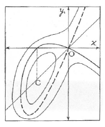
Figure 2: A schematic diagram of the model problem. The curve given by Eq. (16) passes through the origin for $c=0$. For this critical trajectory $\rm{O}$ is a saddle point while $\rm{C}$ is a centre type fixed point. This figure differs from Fig.1 by a tilt of the axes.

We wish to study the evolution of the system from the initial condition $y=0$ for all $x$ at $t=0$. For small $x$, dropping the $x^{3}$ term again, allows us to determine the form of the function $F$ as $F(z)=-3(2-\sqrt{3})z^{2}$. The solution, consequently, becomes

$$y^{2}-2xy-2x^{2}-{\frac{2}{3}}x^{3}=-3\left(2-\sqrt{3}\right)\left[x+\sqrt{{\frac{\left(y-x\right)^{2}}{3}}-\frac{2}{9}x^{3}}\right]^{2}e^{-2{\sqrt{3}}t}$$ (21)

and as $t{\longrightarrow}{\infty}$, we select the separatrices given by

$$y^{2}-2xy-2x^{2}-{\frac{2}{3}}x^{3}=0$$ (22)

a result whose remarkable feature is worth stressing. The evolution started far away from the separatrix. In fact, it started as $y=0$ for all $x$ at $t=0$. The evolution proceeded through a myriad of stationary states (all arguably stable under a linear stability analysis) and then locked on to the separatrix. Our claim is that this dynamic mechanism selects the velocity profile in the practical situation as well, and this is entirely in consonance with a similar and well established selection mechanism for the spherically symmetric flow [3].

5 Concluding remarks

In a previous section we discussed that linear stability analysis of the stationary inflow solutions offers no direct clue as to the preference of the disc system for a particular stationary solution. However, in a somewhat indirect approach to this issue we could make use of a linear stability analysis to have a feel for the special feature of the critical solution. A very convenient way of carrying out the linear stability analysis is in terms of the variable ${\phi}={\rho}^{(\gamma+1)/2}vR^{5/2}$ [12]. In terms of this variable, the perturbation equation for $\phi$ reads

$${\frac{{\partial}^{2}{\phi}^{\prime}}{\partial t^{2}}}+2{\frac{\partial}{\partial R}}\left({v_{0}}{\frac{\partial{\phi}^{\prime}}{\partial t}}\right)+{\frac{1}{v_{0}}}{\frac{\partial}{\partial R}}\left[{v_{0}}\left({v_{0}}^{2}-{\frac{2}{\gamma+1}}{c_{s0}}^{2}\right){\frac{\partial{\phi}^{\prime}}{\partial R}}\right]=0$$ (23)

in which ${\phi}^{\prime}$ is the perturbation on the steady solution of $\phi$, and the subscripted label $0$ indicates steady state values wherever in use [12].

In a spacetime with metric $g^{\mu\nu}$, the wave equation for a scalar variable is [14]

$$\frac{\partial}{\partial x^{\mu}}\left(g^{\mu\nu}\frac{\partial\phi^{\prime}}{\partial x^{\nu}}\right)=0$$ (24)

Ignoring the angle variables, and using the notation that ${\mu}=1$ corresponds to $t$ and ${\mu}=2$ corresponds to $R$, we have the identification

$$g^{11}=1,\,\,g^{12}=g^{21}={v_{0}},\,\,g^{22}={v_{0}}^{2}-{\frac{2}{\gamma+1}}{c_{s0}}^{2}$$ (25)

The effective covariant components are

$$g_{11}=1-{\frac{{v_{0}}^{2}}{{\tilde{c_{s0}}}^{2}}},\,\,g_{12}=g_{21}={\frac{v_{0}}{{\tilde{c_{s0}}}^{2}}},\,\,g_{22}=-{\frac{1}{{\tilde{c_{s0}}}^{2}}}$$ (26)

in which ${\tilde{c_{s0}}}=\sqrt{2}(\gamma+1)^{-1/2}{c_{s0}}$.

The differential distance in the metric space has the form

$$ds^{2}={\frac{1}{{\tilde{c_{s0}}}^{2}}}\left[{{\tilde{c_{s0}}}^{2}}dt^{2}-\left(dx^{i}-{{v_{0}}^{i}}dt\right){{\delta}_{ij}}\left(dx^{j}-{{v_{0}}^{j}}dt\right)\right]$$ (27)

and this is to be compared with the Painlevé-Gullstrand form of $ds^{2}$ for a rotating black hole of mass $\tilde{M}$

$$ds^{2}=dt^{2}-\left(dr{\pm}{\sqrt{{\frac{2G{\tilde{M}}}{r}}-{\frac{L^{2}}{r^{2}}}}}dt\right)^{2}+{r^{2}}d{\theta}^{2}$$ (28)

We now note from Eq. (7) that at the sonic point, ${v_{c}}^{2}=(2/5)[(GM/{R_{c}})-(L/{R_{c}})^{2}]$, and hence in the vicinity of the sonic point the metric implied by the linear stability analysis of the stationary solution appears quite close in form to the metric of a rotating black hole. The unidirectional nature of trajectories near a black hole suggests that trajectories go through the sonic point, which is equivalent to saying that transonic trajectories will be chosen.

In concluding we would also like to comment on the nature of the possible critical point(s) when we consider the more likely case of a disc with a mechanism for the outward transport of angular momentum. It is possible with the help of Eq. (6) to expand and linearize about the critical point value of the angular velocity $\Omega$, but without any knowledge of an exact dependence of $\Omega$ on $R$, there would be no way of fixing the critical point(s). However it can be conceived that as an extension of the inviscid case, there may be multiple parameter-dependent critical points [15] and in that event at least one of them may be saddle type, with all its associated difficulties within the stationary framework itself. In that event, once again the selection mechanism has to be time evolutionary in nature.

References

- [1] S. K. Chakrabarti, Theory of Transonic Astrophysical Flows (World Scientific, Singapore, 1990)
- [2] H. Bondi, On spherically symmetrical accretion, Monthly Notices of the Royal Astronomical Society 112, 195 (1952)
- [3] A. K. Ray and J. K. Bhattacharjee, Realizability of stationary spherically symmetric transonic accretion, Physical Review E 66, 066303 (2002) astro-ph/0212558
- [4] M. A. Abramowicz and W. H. Zurek, Rotation-induced bistability of transonic accretion onto a black hole, The Astrophysical Journal 246, 314 (1981)
- [5] D. Molteni, H. Sponholz, and S. K. Chakrabarti, Resonance oscillation of radiative shock waves in accretion disks around compact object, The Astrophysical Journal 457, 805 (1996)
- [6] S. K. Chakrabarti, Standing Rankine-Hugoniot shocks in the hybrid model flows of the black hole accretion and winds, The Astrophysical Journal 347, 365 (1989)
- [7] J. Frank, A. King, and D. Raine, Accretion Power in Astrophysics (Cambridge University Press, Cambridge, 1992)
- [8] R. Narayan and I. Yi, Advection-dominated accretion : A self-similar solution, The Astrophysical Journal 428, L13 (1994)
- [9] N. I. Shakura and R. A. Sunyaev, Black holes in binary systems. Observational appearance, Astronomy and Astrophysics 24, 337 (1973)
- [10] S. Chandrasekhar, An Introduction to the Study of Stellar Structure (The University of Chicago Press, Chicago, 1939)
- [11] D. W. Jordan and P. Smith, Nonlinear Ordinary Differential Equations (Clarendon Press, Oxford, 1977)
- [12] A. K. Ray, Linearized perturbation on stationary inflow solutions in an inviscid and thin accretion disc, Monthly Notices of the Royal Astronomical Society 344, 83 (2003) astro-ph/0212515
- [13] L. Debnath, Nonlinear Partial Differential Equations for Scientists and Engineers (Birkhäuser, Boston, 1997)
- [14] M. Visser, Acoustic Black Holes: Horizons, Ergosphere and Hawking Radiation, Classical and Quantum Gravity 15, 1767 (1998) gr-qc/9712010
- [15] S. K. Chakrabarti, Grand unification of solutions of accretion and winds around black holes and neutron stars, The Astrophysical Journal 464, 664 (1996)