The extended tails of Palomar 5: A ten degree arc of globular cluster tidal debris

Abstract

Using wide-field photometric data from the Sloan Digital Sky Survey (SDSS) we recently showed that the Galactic globular cluster Palomar 5 is in the process of being tidally disrupted. Its tidal tails were initially detected in a 2.5 degree wide band along the celestial equator. A new analysis of SDSS data for a larger field now reveals that the tails of Pal 5 have a much larger spatial extent and can be traced over an arc of 10^∘ on the sky, corresponding to a projected length of 4 kpc at the distance of the cluster. The tail that trails behind the Galactic motion of the cluster fades into the field at an angular distance of $6\fdg 5$ from the cluster center but shows a pronounced density maximum between $2^{\circ}$ and $4^{\circ}$ from the center. The leading tail of length $3\fdg 5$ extends down to the border of the available field and thus presumably continues beyond it. The projected width of these tails is small and almost constant (FWHM $\sim$ 120 pc), which implies that they form a dynamically cold and hence long-lived structure. The number of former cluster stars found in the tails adds up to about 1.2 times the number of stars in the cluster, i.e. the tails are more massive than the cluster in its present state. The radial profile of stellar surface density in the tails follows approximately a power law $r^{\gamma}$ with $-1.5\leq\gamma\leq-1.2$.

The stream of debris from Pal 5 is significantly curved, which demonstrates its acceleration by the Galactic potential. The stream sets tight constraints on the geometry of the cluster’s Galactic orbit. We conclude that the cluster is presently near the apocenter but has repeatedly undergone disk crossings in the inner part of the Galaxy leading to strong tidal shocks. Using the spatial offset between the tails and the cluster’s orbit we estimate the mean drift rate of the tidal debris and thus the mean mass loss rate of the cluster. Our results suggest that the observed debris originates mostly from mass loss within the last 2 Gyrs. The cluster is likely to be destroyed after the next disk crossing, which will happen in about 100 Myr. There is strong evidence against the suggestion that Pal 5 might be associated with the Sgr dwarf galaxy.

1 Introduction

Globular clusters are the oldest stellar systems commonly found in the Milky Way, having typical ages of 12 to 15 Gyr. They thus represent fossil relics from the early formation history of the Galaxy. However, the globular clusters we see today are probably not representative of the system of Galactic globular clusters at early stages. They may in fact be the selected ’survivors’ of an initially much more abundant population. Analytic estimates and numerical experiments predict that on time scales of Gigayears globular clusters undergo external and internal dynamical evolution, by which they may suffer a permanent loss of members, and eventually dissolve.

One of the major factors governing the dynamical evolution of those clusters is the Galactic tidal field. The tidal field has two important effects: (1) It creates drains through which stars are carried away from the outer part of the cluster, and hereby truncates the bound part of the cluster to a certain spatial limit (von Hoerner 1957, King 1962). (2) It feeds energy into the cluster through so-called tidal shocks, i.e., rapid variations of the strength of the external forces which occur during crossings of the Galactic disk or close passages of the Galactic bulge (Ostriker, Spitzer, & Chevalier 1972, Kundic & Ostriker 1995). Detailed simulations of globular cluster dynamics for a variety of masses and internal structures and different types of orbits in different Galactic model potentials have shown that tidal shocks accelerate the dynamical evolution of globular clusters and enhance their mass loss in such a way that 50% or more of the present-day globulars will be destroyed within the next Hubble time (Gnedin & Ostriker 1997, including disk-shocks; Baumgardt & Makino 2002, using a model without disk). Similarly, it has been shown that the present sample of globular clusters is most likely the remainder of an initially much more numerous system of clusters, many of which are meanwhile dissolved (Murali & Weinberg 1997, Fall & Zhang 2001). In this way, the spatial distribution, kinematics, and mass function of the globular cluster system may have changed a lot. Also, the shape of the stellar mass function of individual clusters may have changed considerably since their formation because of preferential depletion of low-mass stars as a result of mass segregation (Baumgardt & Makino 2002).

Observations suggest that the Milky Way globular clusters are indeed spatially truncated by the Galactic tidal field. Measurements of the radial surface density profiles or surface brightness profiles of globular clusters (e.g., King et al. 1968; Trager, King & Djorgovski 1995) showed that many globulars have profiles that decline more steeply than a power law and, by extrapolation, suggest the existence of a finite boundary. Their profiles are often well fit by King (1966) models, which are of finite size. The estimated limiting radii obtained by extrapolation with King models were found to correlate with the clusters’ galactocentric distances, and the way in which they correlate agrees to what would be expected for tidal radii in a Galaxy with a flat rotation curve (Djorgovski 1995). Nevertheless, a firm observational proof for the predicted mass loss and dissolution of globular clusters in the Galactic tidal field has been missing until recently.

Using color-magnitude selected star counts, Grillmair et al. (1995) measured the stellar surface densities of a number of globular clusters to lower levels and hence larger radii than earlier studies. They then found that at very low levels (typically more than four orders of magnitude below the central surface density) the observed profiles frequently exceed the prediction from King models and extend beyond the limiting radius of these models. Similar results were obtained by Lehmann & Scholz (1997), Testa et al. (2000), Leon et al. (2000), and Siegel et al. (2001). The observed departures from King models are in some cases associated with a break in the logarithmic slope of the profile, which resembles the results of numerical simulations of globular clusters, where a break in the radial surface density profile marks the transition between the bound part and the unbound part of the cluster population (e.g., Oh & Lin 1992, Johnston et al. 1999a). Hence, these observations suggest that many clusters are surrounded by weak haloes or tails of unbound stars that might result from tidal stripping. On the other hand, the two dimensional surface density distributions obtained by Grillmair et al. (1995), Testa et al. (2000), and Leon et al. (2000) did not clearly confirm this suggestion and left doubts about the reality of the observed structures because these were in most cases too complex and diffuse to be unambiguously identifiable as tails of tidal debris. In fact, contamination by galaxy clustering in the background or by variable extinction across the field may have lead to spurious detections of such tails. The latter was recently demonstrated by Law et al. (2003) for the low-latitude cluster $\omega$ Cen.

Among the much bigger and more massive dwarf spheroidal (dSph) satellites in the Milky Way halo, there has been growing evidence that at least the Sagittarius dSph, which is the nearest of these systems, is subject to very substantial mass loss and produces strong tails of tidal debris. The stellar stream from this dSph has meanwhile been detected around the whole celestial sphere (see Majewski et al. 2003 and references therein).

Turning back to the globular clusters, deep small-field studies with the Hubble Space Telescope (HST) revealed that several of the Galactic globulars have luminosity functions that are unusually flat or even decreasing towards the low-luminosity end (Piotto, Cool, & King 1997; De Marchi et al. 1999; Piotto & Zoccali 1999; Grillmair & Smith 2001). This deficiency in low-mass stars could be an indication of tidal mass loss (when combined with mass segregation in the cluster) and has frequently been interpreted in this sense. However this is not by itself a proof of tidal mass loss because (1) the observations do not necessarily represent the overall luminosity function of the cluster (spatial variations due to mass segregation, either dynamical or primordial), and (2) it might be possible that intrinsic differences exist between the overall luminosity functions of different clusters.

The evolution of a cluster depends on its internal parameters and its orbit. Ostriker & Gnedin (1997) presented so-called ’vitality diagrams’ for globular clusters in the parameter space of half-mass radius, mass, and Galactocentric distance, showing in which region of this space a cluster should lie in order to survive more than 10 Gyr. Clusters that do not lie in this region, and hence are expected to dissolve due to disk- and bulge shocks, are those with large half-mass radius and low mass. An extreme example for such an object is the sparse cluster Palomar 5, which has a mass of less than $10^{4}M_{\odot}$ and a half mass radius of about 20 pc. Since Pal 5 is also one of the clusters that were found to have an atypically flat luminosity function (Smith et al. 1986, Grillmair & Smith 2001) it presents a particularly interesting test case for tidally-induced mass loss.

The commissioning of the Sloan Digital Sky Survey (SDSS; York et al. 2000) provided deep multi-color CCD imaging in $2.5^{\circ}$ wide stripe across Pal 5. This allowed a wide-field search for cluster stars in the surroundings of Pal 5 (Odenkirchen et al. 2001a, hereafter Paper I). A previous investigation of Pal 5 using photographic plates (Leon et al. 2000) had been compromised by severe problems with contamination from background galaxies. The SDSS observations, however, enabled excellent separation between stars and background galaxies and an efficient selection of cluster stars by color and magnitude. We found strong evidence for two massive tails of tidal debris emerging from Pal 5. These tails showed a well-defined characteristic shape and were found to contain about half as much mass as the cluster.

The detection of such tails with clearly identifiable structure has two important aspects: (1) It provides conclusive, direct proof for on-going tidal mass loss in a globular cluster. (2) It reveals unique information on the orbit of the cluster and opens a very promising way for investigating the gravitational potential in the Galactic halo (e.g., Murali & Dubinski 1999, Johnston et al. 1999b). In the present paper we describe the analysis of further SDSS data for a more than five times larger field around Pal 5, which have become available since Paper I. The goal of this study is to trace the tidal debris of Pal 5 to larger distances from the cluster in order to obtain a more complete census of its mass loss and to constrain the basic properties of the distribution of the debris such as its shape and density profile. As we will show, Pal 5 is the first globular cluster that exhibits fully-fledged tidal tails with a total angular extent of $10^{\circ}$ on the sky.

In §2 we provide details about the observations and the photometric data derived from them. §3 describes the methods used to analyse the data. In §4 we present the resulting surface density distribution of cluster stars and describe the basic features of the tidal tails. §5 deals with the determination of the cluster’s local orbit and its extrapolation to a global scale. In §6 we derive estimates of the mass loss rate and the total mass loss of the cluster. The results are discussed and summarized in §7, and a brief outlook on future work is given in §8.

2 Observations

The SDSS is a large deep CCD survey designed to cover 10,000 square degrees of sky by imaging in five optical passbands, and by spectroscopy. The imaging data are obtained in great-circle drift scans using a large mosaic camera on a dedicated 2.5m telescope at Apache Point Observatory, Arizona. (For further information on the survey and its technical details see York et al. 2000, Gunn et al. 1998, Fukugita et al. 1996, Hogg et al. 2001, Smith et al. 2002, and Pier et al. 2002).

The data that we use in this study stem from the SDSS imaging runs 745, 752, 1458, 1478, 2190, 2327, 2334, and 2379, carried out between March 1999 and June 2001. The various strips of sky scanned in these runs yield complete coverage of a $6\fdg 5$ to $8^{\circ}$ wide zone along the equator in the right ascension range from $224^{\circ}$ to $236^{\circ}$. Hereby we have multi-color photometry for Pal 5 and its surroundings in a contiguous, trapezium-shaped field with an area of 87 square degrees. The observations reach down to an average magnitude limit of about 23.0 mag in $i^{*}$ and 23.5 mag in $r^{*}$ (approximate limits of 90% incompleteness). Photometric and astrometric data reduction and object classification were done by the standard SDSS image processing pipeline (see Lupton et al. 2001 and Pier et al. 2002 for different parts of the pipeline). The photometry used here is from before the public data release DR1 and hence does not precisely match the final SDSS photometric system. However, the preliminary photometric calibration of the data is spatially uniform to about 3% (Stoughton et al. 2002). The lack of the final calibration does not affect our study since we use the photometry in a purely empirical and differential way.

Our investigation is restricted to objects classified as unresolved sources (thus eliminating a large number of background galaxies that would otherwise contaminate the star counts) and uses object magnitudes derived by point-spread function (PSF) fitting. The median internal errors of the magnitudes in $g^{*}$, $r^{*}$, and $i^{*}$ are 0.015 mag or better for stars brighter than 18.0 mag (in $g^{*},r^{*},i^{*}$ respectively), rise to values between 0.023 and 0.035 mag at magnitude 20.0, and reach the level of 0.10 to 0.17 mag at magnitude 22.0. We confirmed these errors by analysing repeated measurements in overlapping scans. The median differences between magnitudes from independent observations are between $1.0\times$ and $1.2\times$ the median internal errors, showing that the quoted median errors provide reliable estimates of the photometric accuracy of these data.

According to the dust maps of Schlegel, Finkbeiner & Davis (1998) the southern and south-eastern part of the field is affected by a considerable amount of interstellar extinction while in the northwestern part the extinction is much lower. More specifically, the extinction in the $g$ band varies from 0.15 mag at the northern edge to 0.75 mag at the southern edge of the field. This corresponds to variations in the reddening of the color index $g-i$ in the range $0.07\leq E(g-i)\leq 0.34$. To remove these variations from the observed magnitudes we applied individual extinction corrections derived from the local $E(B-V)$ reddening given by Schlegel, Finkbeiner & Davis. The resulting dereddened magnitudes should properly be named $g_{0}^{*}$ etc., however, for simplicity, we will suppress the index 0 here. Since the reddening data from Schlegel et al. represent the integrated extinction along the entire line of sight, the magnitudes of stars that are in front of the bulk of intervening material would in this way become overcorrected. However this is unlikely to happen for stars belonging to Pal 5, which are located more than 20 kpc from the sun and seen far behind the northern part of the Galactic bulge. Color-magnitude diagrams for different parts of the field with different amounts of extinction show, that there is no sign of overcorrection in the blue edge (main-sequence turn-off) of the halo field star population. In the case of significant overcorrection this edge would be inclined to the blue with increasing brightness, which is not observed.

Due to variations in the observing conditions the completeness of object detection at faint magnitudes is somewhat different from run to run. This causes artificial inhomogeneities in the stellar surface density of the faintest stars. In order to avoid such effects it was necessary to cut the sample at $i^{*}=21.8$ mag. At the bright end we chose a threshold of $i^{*}=15.0$ mag because brighter stars risk to have saturated images and because none of the giants in Pal 5 is brighter than this limit. The resulting data set contains about 940,000 point sources.

3 Photometric object filtering

3.1 Unfiltered sample

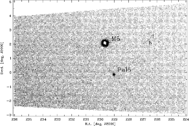
Figure 1: Map of the surface density of SDSS point sources with $i^{*}\leq 21.8$ mag in the region of Pal 5 (plotted vs. right ascension, declination). The density peak at position (229$\fdg$0,$-$0$\fdg$1) shows the cluster Pal 5 while the ring around position (229$\fdg$6,+2$\fdg$1) is due to the cluster M 5 (central part incomplete because of strong crowding). Weak traces of tidal debris from Pal 5 can be recognized northeast and southwest of the cluster. The arrow labeled with $b$ indicates the direction of increasing galactic latitude. For further details see §3.1.

The full set of SDSS point sources with magnitudes in the range $15.0\leq i^{*}\leq 21.8$ has an average surface density of 3.0 stars per arcmin² and a large-scale surface density gradient of 0.13 stars per arcmin² per degree in the direction of decreasing galactic latitude. Figure 1 shows a map of the stellar surface density derived by source counts in pixels of $3^{\prime}\times 3^{\prime}$. There are two strong local density enhancements in this field, at positions ($229\fdg 0$,$-0\fdg 1$) and (229$\fdg$6,$+2\fdg 1$) in right ascension, declination (J2000). The first one represents the remote cluster Pal 5 while the second one is due to the much closer and much richer globular M 5. The latter is not relevant for this paper, except that one must avoid this region when investigating the properties of the general field around Pal 5. The peak surface density of cluster stars in the center of Pal 5 is 25.2 arcmin^-2, i.e., $8.4\times$ the mean density of the surrounding field.

Figure 1 also reveals an arc of very weak overdensity extending northeast and southwest of Pal 5. The results that we will present in §4.1 confirm that these are rudimentary traces of extended debris from Pal 5. This is remarkable since it means that weak traces of the cluster’s debris are visible even without any particular photometric filtering. However, the surface density of these features is only on the level of $1\sigma$ (rms of surface density in individual pixels) above the local mean surface density of the field.

In order to get detailed information on the distribution of stars from Pal 5 one needs to enhance the contrast between the cluster and the field, in particular the dominating Galactic foreground. To first order, this can be achieved through simple cuts in color and magnitude. A more efficient variant of this method is to use an appropriately shaped polygonal mask in color-magnitude (hereafter c-m) space. This approach was taken, e.g., by Grillmair et al. (1995), Leon et al. (2000), and in Paper I in the context of globular clusters, and also by Majewski et al. (2000) and Palma et al. (2003) in the context of dwarf spheroidal (dSph) galaxies. However, sharply defined cuts or windows in c-m space do still not provide the optimal method to map out the spatial distribution of the stellar population of Pal 5 because each star is treated as either a definite member or a definite non-member of the cluster population. This does not completely exploit the available information. Since the photometry actually allows us to derive smoothly varying membership probabilities as a function of color and magnitude one can optimize the object filtering by using these probabilities.

3.2 Optimal contrast filtering

A straight-forward way to make comprehensive use of the photometric information is to construct empirical c-m density distribution templates $f_{C}(m,c)$, $f_{F}(m,c)$ for the cluster and the field ($m$ and $c$ denoting magnitude and color index), and to use these to determine the surface density $\Sigma_{C}$ of the cluster population for each position in the field by a weighted least-squares adjustment. This kind of approach was, e.g., described by Kuhn, Smith, & Hawley (1996) in a study of the Carina dSph, and recently discussed in more detail by Rockosi et al. (2002), who used it for an analysis of a smaller SDSS data set on Pal 5. The adjustment is done such that the weighted sum of field stars plus cluster stars yields the best approximation of the observed total c-m distribution. In the present study we have applied this method of optimal data filtering in the following way:

Using the magnitudes $g^{*}$, $r^{*}$, and $i^{*}$ (which provide higher accuracies than $u^{*}$ and $z^{*}$), we first defined orthogonal color indices $c_{1}$ and $c_{2}$ as in Paper I:

$$c_{1} = \ 0.907(g^{*}-r^{*})+0.421(r^{*}-i^{*})\ \$$ (1a)

$$c_{2} = -0.421(g^{*}-r^{*})+0.907(r^{*}-i^{*})\ \$$ (1b)

The choice of the indices is such that the main axis of the almost one-dimensional locus of Pal 5 stars in the $(g-r)$ versus $(r-i)$ color-color plane lies along the $c_{1}$-axis while the $c_{2}$ axis is perpendicular to it. We then preselected the sample in $c_{2}$ by discarding all objects with $|c_{2}|>2\sigma_{c_{2}}(i^{*})$, where $\sigma_{c_{2}}(i^{*})$ is the rms dispersion in $c_{2}$ for stars of magnitude $i^{*}$ in Pal 5. Stars with these $c_{2}$ colors are unlikely to be from the cluster. We also preselected in $c_{1}$ by restricting the sample to the range $0.0\leq c_{1}\leq 1.0$ because one expects very few stars of the cluster population outside this range.

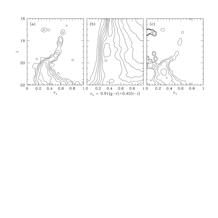
Figure 2: Hess diagrams showing the normalized densities of the stellar population of Pal 5 (a) and of the field stars around Pal 5 (b) in the plane of color index $c_{1}$ and magnitude $i^{*}$, and the ratio of cluster to field as a function of color and magnitude (c). In panels (a) and (c) the contour levels increase by factors of 2 from one contour to the next. Panel (b) shows contours on equidistant levels.

Next we constructed c-m density diagrams (Hess diagrams) for the cluster and the field by sampling the stars that lie within $12^{\prime}$ from the center of Pal 5 (cluster diagram) and those that are more than $1^{\circ}$ away from the location of the stream and outside M 5 (field diagram) on a grid in the plane of $c_{1}$ and $i^{*}$. Bins of 0.01 mag$\times$ 0.05 mag were used and the counts were smoothed with a parabolic kernel of radius 3 pixels. The cluster c-m distribution was corrected for the presence of field stars in the $12^{\prime}$ circle around the cluster center by subtracting the field c-m distribution in appropriate proportion. The resulting diagrams of the normalized c-m densities $f_{C}$, $f_{F}$ of cluster stars and field stars are shown in Figures 2a and 2b. The cluster members are concentrated along well-defined branches (giant branch, horizontal branch, subgiant branch and main sequence) while the field star distribution is more diffuse, showing local maxima along $c_{1}\approx 0.4$, which can be attributed to the turn-off region of thick disk and halo. By comparing the field star c-m distribution in the region northwest of the cluster to that in the region southeast of the cluster it appears that $f_{F}$ is not strictly constant over the field. However, the differences are not dramatic because the deviations from the mean distribution are mostly below 10%. Since a more local estimate of $f_{F}$ can only be obtained at the cost of higher noise or lower c-m resolution we preferred to neglect the spatial variations and to work with the mean distribution shown in Figure 2b.

In order to derive the surface density distribution of cluster stars on the sky one needs a mathematical model that provides a link to the observed distributions. The general ansatz for the stellar density in the hyperspace spanned by the celestial sphere and the c-m plane is a sum of densities $S_{C}$ and $S_{F}$ for the cluster and the field (i.e., non-cluster stars)

$$S(\alpha,\delta,m,c) = S_{C}+S_{F}$$ (2a)

$$S_{C} = \Sigma_{C}(\alpha,\delta)\Phi_{C}(m,c)$$ (2b)

$$S_{F} = \Sigma_{F}(\alpha,\delta)\Phi_{F}(\alpha,\delta,m,c)$$ (2c)

where each component can be split up into a product of a surface density $\Sigma$ on the sphere and a position-dependent normalized c-m density $\Phi$. ($\alpha,\delta$ denote coordinates on the celestial sphere, $m$ and $c$ denote magnitude and color index.) For the cluster component as a sample of stars of common origin we assume that (1) it is everywhere composed of the same mix of stellar types and that (2) all stars are at practically the same distance from the observer. This implies that $\Phi_{C}$ does in fact not depend on position ($\alpha,\delta$) (as in equation 2b). In contrast to this the field component is an inhomogeneous sample, i.e., its composition by stars of different types and its density distribution along the line of sight are spatially variable, so that $\Phi_{F}$ must in principle vary with position on the sky (equation 2c).

Let $j$ be an index labelling the pixels of a grid in the c-m plane and $k$ be an index labelling the positions $(\alpha_{k},\delta_{k})$ of a grid on the sky, then the number $\nu(k,j)$ of stars lying in a solid angle $\Omega_{k}$ centered on $(\alpha_{k},\delta_{k})$ and with magnitude and color falling on the pixel $j$ of area $P_{j}$ is obtained by integrating equation (2a) over $\Omega_{k}$ and $P_{j}$, i.e.

$$\nu(k,j) = \nu_{C}(k)f_{C}(j)+\nu_{F}(k)f_{F}(k,j)\quad$$ (3)

$$\mathrm{where}$$

$$\nu_{\,C,F}(k) = \int_{\Omega_{k}}S_{\,C,F}\ d\Omega$$

$$f_{C}(j) = \int_{P_{j}}\Phi_{C}\ dm\,dc$$

$$f_{F}(k,j) = \frac{1}{\nu_{F}(k)}\int_{\Omega_{k}}\int_{P_{j}}\Phi_{F}\ dm\,dc\,d\Omega$$

Although $f_{F}$ does in principle depend on position index k, this dependence is in our case not important because we can assume that substantial changes in the characteristics of the field population occur only on larger scales and that hence (as the observations show) $f_{F}$ is approximately constant within the chosen field. The distributions $f_{C}$ and $f_{F}$ in the model of equation (3) can thus be represented by the above normalized average c-m distributions that have been drawn from the observations. $\nu_{C}(k)$ and $\nu_{F}(k)$ are the numbers of cluster stars and field stars in $\Omega_{k}$, the former of them being the target of our analysis. Apart from observational noise (and apart from small deviations due to spatial variations in the c-m distribution of the field stars, which the model neglects), the left hand side of equation (3) should correspond to the observed star counts $n(k,j)$ in $\Omega_{k}\times P_{j}$. Thus one can plug in $n(k,j)$ for the expected number $\nu(k,j)$ in equation (3). Equation (3) then does not have an exact solution. However, we can determine a least-squares solution for $\nu_{C}(k)$ by demanding that the square sum of the noise-weighted deviations between the observed number $n(k,m)$ and the expected number $\nu(k,m)$ given by the right hand side of equation (3), summed up over the c-m grid, is minimal. Since the contribution of the cluster population to the total counts is small (outside the cluster) we assume the noise to be dominated by the field stars, i.e., we expect $\sigma_{n}^{2}(k,m)=\nu_{F}(k)f_{F}(m)$. The sum of weighted squares to be minimized thus is:

$$\chi^{2}(k)=\hskip 156.49014pt$$ (4)

$$\quad\sum_{j}\frac{\left(n(k,j)-\nu_{C}(k)f_{C}(j)-\nu_{F}(k)f_{F}(j)\right)^{2}}{\nu_{F}(k)f_{F}(j)}$$

It is straightforward to calculate (via $d\chi^{2}/d\nu_{C}=0$) that the least-squares solution for $\nu_{C}(k)$, which we call $n_{C}(k)$, and its variance $\sigma^{2}_{n_{C}}(k)$ are:

$$n_{C}(k)=\frac{\displaystyle\left(\sum_{j}n(k,j)\frac{f_{C}(j)}{f_{F}(j)}\right)-n_{F}(k)}{\displaystyle\sum_{j}\frac{f_{C}^{2}(j)}{f_{F}(j)}}$$ (5a)

$$\sigma^{2}_{n_{C}}(k)=\quad n_{F}(k)\bigg{/}\sum_{j}\frac{f^{2}_{C}(j)}{f_{F}(j)}\qquad$$ (5b)

In principle, one could determine both $n_{C}$ and $n_{F}$ (i.e., the best estimate for $\nu_{F}$) in this way by minimizing the $\chi^{2}$ of equation (4). However, for $\nu_{F}$ we already know (or can safely assume) that it must be a smoothly varying function of position that can be described by a simple (polynomial) model. Thus we preferred to use this constraint to determine $n_{F}$ externally (for practical details see §4.1) and not in a simultaneous least-squares adjustment with $\nu_{C}$. This makes the solution for $\nu_{C}$ more robust.

Equation (5a) allows the following interpretation: One finds the least-squares solution $n_{C}(k)$ by weighting each star in the solid angle $\Omega_{k}$ by the quotient $w(j)=f_{C}(j)/f_{F}(j)$ according to its position in the c-m plane, summing up the weights of all stars, and dividing this sum by the factor $a=\sum_{j}(f_{C}^{2}/f_{F})$. This yields the estimated number of cluster stars $n_{C}$ plus a term $n_{F}/a$, i.e., the estimated number of field stars attenuated by $a$. By subtracting this residual field star contribution one obtains $n_{C}$. Equation (5b) shows that the variance of $n_{C}$ is reduced to $1/a$ times the variance of the field star counts. In other words, the noise in the determination of the surface density of cluster stars decreases by the factor $\sqrt{a}$. The weight function $w=f_{C}/f_{F}$ is shown by the contour plot in Figure 2c. We obtain an attenuation factor $a=5.1$ and hence a noise reduction of $\sqrt{a}=2.3$ with respect to the unfiltered, but preselected sample. In total, i.e., in comparison with the full sample, the noise level is reduced by a factor of 4.3.

4 The tidal stream

4.1 Surface density map

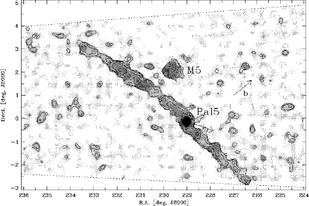
Figure 3: Map of the surface density of stars that are photometrically concordant with the stellar population of Pal 5 (plotted in equatorial coordinates ra,dec). These surface densities were derived by least-squares estimation as described in §3.2. The lowest contours show density levels of $1.5\sigma$, $2\sigma$, $3\sigma$, and $5\sigma$ above zero (white). Pal 5 is seen to be accompanied by two long tidal tails. The tidal debris covers an arc of almost 10^∘ (for further details see §4.1). The arrow attached to Pal 5 gives an approximate indication of the direction of its galactic motion based on the proper motion measurement by Cudworth (see §5.2). The arrow labeled with $b$ shows the direction of increasing galactic latitude. The patch of enhanced density around (229$\fdg$6,+2$\fdg$1) is a residual feature from the cluster M 5 and hence not related to Pal 5. The dotted lines mark the borders of the field.

We constructed a map of the stellar surface density of Pal 5 stars by applying the above method of least squares estimation on a grid with pixels of $3^{\prime}\times 3^{\prime}$ in the plane of the sky. The residual contribution from field stars was determined by fitting a bi-linear background model to the weighted counts in those pixels that are at least $1^{\circ}$ away from the cluster and the tails, and also away from M 5. After pre-selection and weighting, the mean surface density of the field stars is 0.16 arcmin^-2 and the surface density gradient across the field is about $5\times 10^{-3}$ arcmin^-2 per degree. By subtracting the best-fit bi-linear background model the density distribution in the field becomes essentially flat. For further reduction of the noise the counts were smoothed by weighted averaging with a parabolic kernel of radius 4 pixels. In regions with surface density above the 5$\sigma$ level we used a kernel with a smaller radius to preserve higher resolution. Figure 3 presents the resulting surface density map as a grey scale and contour plot in equatorial celestial coordinates (i.e., right ascension and declination).

This map shows a striking coherent structure that is spatially connected to the main body of Pal 5 and has stellar surface densities varying from $1.5\sigma$ up to $5\sigma$ ($\sim$ 0.12 arcmin^-2) and higher. The geometry relative to the cluster clearly identifies this structure as debris from Pal 5. The debris forms two long narrow tails on opposite sides of the cluster and extends over an arc of about 10^∘. This corresponds to a projected length of 4 kpc at the distance of the cluster. The tails have a width of about $0\fdg 7$ in projection on the plane of the sky. Apart from small scale variations the width of the tails does not systematically change with angular distance from the cluster. The northern tail, which - as will be shown later in §5.2 - is trailing behind the cluster, is traced out to an angular distance of at least $5\fdg 8$ from the center of the cluster, but possibly out to $6\fdg 5$, and appears slightly curved. The maximum surface density of stars in this tail is about 0.2 arcmin^-2. It occurs at angular distances between $2\fdg 2$ and $3\fdg 7$ from the cluster center and was hence not covered by the initial detection of the tails in Paper I.

The southern tail, which is the one that leads the motion of the cluster (see §5.2), is seen over $3.6^{\circ}$ and reaches down to the edge of the currently available field. This suggests that the tail continues beyond this limit, as one would indeed expect when assuming approximate point symmetry in the distribution of debris with respect to the cluster. The southern tail exhibits density maxima at angular distances of $1\fdg 6$ and $3\fdg 5$ from the cluster center, which are, however, less pronounced than in the northern (trailing) tail. The transition between the cluster and the tails is not straight. Instead we see a characteristic S-shape in the distribution of stars, which closely resembles the structures seen in simulations of disrupting globular clusters and satellites (e.g., Combes et al. 1999, Johnston et al. 2002). This S-shape feature clearly indicates that the stars are stripped from the outer part of the cluster by the Galactic tidal field dragging them away in the direction towards the Galactic center and anticenter.

Besides the two tails of Pal 5 and a spurious patch of high stellar density left over from the cluster M 5, the map shows a number of small isolated patches with densities on the level of $2\sigma$ above zero, which are dispersed over the field. These are most likely not traces of the population of Pal 5 but the result of random fluctuations in the distribution of field stars. To test this we generated random fields with the same mean density as the observed residual field star density and sampled these artificial fields in exactly the same way as done with the observations. This Monte Carlo experiment showed that random fields yield $2\sigma$-patches of the same size and with very similar number densities as in Figure 3. As another statistical test we resampled the observations on a grid of non-overlapping pixels with a size of $9^{\prime}\times 9^{\prime}$ and determined the frequency distribution of pixel counts in those regions that lie outside the clusters M 5 and Pal 5 and the tails of Pal 5. This distribution closely agrees with the expected Poisson distribution for a random field of the given mean density (see similar tests of fluctuations described in Odenkirchen et al. 2001b). Both tests reveal that the isolated patches in the map of Figure 3 provide no evidence for further significant local overdensities.

In order to estimate the fraction of stars in the tails and in the cluster, we integrated the surface density of Pal 5 stars in a $42^{\prime}$ wide band covering the tails (2.3 times the FWHM of the tails, see §6.1) and in a circle of radius $12^{\prime}$ around the center of the cluster. A somewhat smaller radius than the cluster’s limiting (or tidal) radius of $16^{\prime}$ (Odenkirchen et al. 2002, hereafter Paper II) was used because the bound and unbound part of the cluster overlap in projection on the sky and cannot be strictly separated. We find that the number of stars in the tails is about 1650 while the number of stars in the cluster is about 1350. This yields a number ratio between tails and cluster of $\beta=1.22$. The number of stars seen in the southern (leading) tail is about half the number found in the northern (trailing) tail (i.e., there are about 1100 stars in the northern and about 550 stars in the southern tail). To check these number ratios we also took an alternative approach and performed integrated number counts on a variety of samples defined by different choices of cut-off lines in the c-m plane. Hereby we obtained values for the ratio between the number of stars in the tails and in the cluster in the range from 1.18 to 1.31. It thus appears that $\beta=1.25\pm 0.06$ is a robust estimate for the observed field. Since the tails may easily extend beyond the area currently covered by the SDSS, the ’true’ ratio is likely to be higher. In any case, we can safely conclude that the tails contain more stellar mass than the cluster.

4.2 Density profile along the tail

Since the debris forms a long and relatively thin structure, it makes sense to treat it as a one-dimensional object and to characterize it by its distribution of linear density. To determine this linear density we modelled the central line of each tidal tail by a sequence of short straight-line segments (fitting by eye) and projected all stars within $0\fdg 35$ from the central line perpendicularly onto it. We then performed weighted star counts as described in equation (4a) in bins of the arc length parameter $\lambda$ along the central line, using a bin size of $0\fdg 25$. The field star contribution was determined using the bilinear background model from Section 4.1, and was subtracted from the counts. We thus obtained the density distributions shown in Figure 4 (statistical uncertainty of the number counts indicated by error bars).

The density curve for the northern (trailing) tail (Fig.4a) shows three pronounced maxima, which correspond to extended density clumps around RA $230\fdg 9$, $231\fdg 8$, and $233\fdg 3$ in the map of Figure 3. The linear density at these maxima is about two times as high as it is on average. Apart from those local variations there is a general decline in the density with increasing $\lambda$. The mean density level decreases by roughly a factor of 3 when comparing $\lambda\sim 0\fdg 5$ to $\lambda\sim 6^{\circ}$.

In order to judge the significance of the observed variations we approximate the general trend in the data by fitting a straight line to the innermost five and the outermost five data points (dashed line in Fig.4a). Comparing the data with this line shows that the smaller amplitude variations in the counts lie within the error bars and hence are likely of statistical nature whereas the strong maxima at the above given locations exceed the straight-line model by about 3 times the error bar. Therefore, these maxima are statistically significant and present real substructure in the tail. Two of the clumps may in fact be part of one broad density enhancement because their separation by only one bin of lower density could be the result of statistical fluctuations.

Along the southern (leading) tail (Fig.4b) the linear density is generally lower than in the corresponding part of the northern (trailing) tail. Again, there are local variations which reflect the presence of density clumps in Figure 3. However, these variations have lower amplitude than those occuring in the northern tail, and the deviations from the general trend of the data (fit of straight line to entire set of data points) are thus not highly significant. In particular, the southern (leading) tail shows no obvious counterpart to the broad density enhancement in the northern (trailing) tail. Since the data for the southern (leading) tail cover a smaller range in $\lambda$ there is less information on the large-scale trend of the density. With the exception of the outermost bin the data points seem to suggest a weak outward decrease. On the other hand, taking into account the error bars the counts are also consistent with the assumption of a constant mean density level. In any case, the density curve leaves no doubt that the southern tail must continue beyond the border of the field. The steep rise of the counts in the outermost bin, be it a statistical fluctuation or due to a real clump, shows that the mean density does not drop to zero at this point. Whether or not the linear density at higher $\lambda$ declines in a similar way as seen in the outer part of the northern (trailing) tail is an interesting question that can presently not be answered.

4.3 Radial profile of the surface density

Another way to describe the tidal debris is by determining the radial profile of the surface density, i.e., the azimuthally averaged surface density as a function of distance from the cluster center. This description disregards the fact that tidal tails are not a circularly symmetric structure, but has the advantage to provide a uniform view of both the cluster and the debris. Therefore, observational studies of globular clusters and local dwarf galaxies are often judging the existence of tidal debris in this way, and results of theoretical studies are also frequently presented in this form (e.g., Johnston et al. 1999a, Johnston et al. 2002).

We derived the radial profile of the cluster and the two tails through weighted number counts in sectors of concentric rings. Out to $r=15^{\prime}$ we divided each ring into its northern and southern half. At larger radii we used progressively narrower sectors to bracket the tails and to minimize the influence of the field, but referred the (background corrected) counts to the full area of the corresponding half ring. This yields the profiles shown in Figure 5. For comparison we also show an analogous profile obtained in two cones away from the tidal tails, i.e., at position angles $100^{\circ}\pm 35^{\circ}$ and $280^{\circ}\pm 35^{\circ}$.

It is clearly visible that the tidal debris is distinguished from the cluster by a characteristic break in the slope of the logarithmically plotted radial profile. Outside the cluster’s core region, i.e., at radii $r>3^{\prime}$, the surface density first decreases steeply as a power law $r^{\gamma}$ with exponent $\gamma=-3$. Between $15^{\prime}$ and $20^{\prime}$ there is a transition region where the profile becomes less steep, and from $20^{\prime}$ outwards the decline of the density is similar to a power law with an exponent in the range $-1.5<\gamma<-1.2$. The comparison profile, which has been measured perpendicularly to the tails and should thus not be affected by tidal debris, shows the same $r^{-3}$ power law decline between $3^{\prime}$ and $10^{\prime}$ but falls off more steeply at $r>10^{\prime}$. This shows that perpendicular to the tails the cluster has a well-defined radial limit. A fit of a King profile to these counts suggests a limiting (or tidal) radius of approximately $16^{\prime}$ (see Paper II). This is near to the radius where the overall radial profile shows the break. By comparing the different radial profiles the tidal perturbation of the cluster is noticable from about $r=12^{\prime}$ outwards.

To determine the power law exponent for the outer part of the radial profile we made a weighted least-squares fit to the data points at $r\geq 20^{\prime}$. For the southern (leading) tail this fit yields $\gamma=-1.25\pm 0.06$. For the northern (trailing) tail the use of all data points results in a poor fit with $\gamma=-1.36$. When leaving out the three most discrepant data points, which describe the strong local density maximum in the range $140^{\prime}<r<220^{\prime}$, we obtain an acceptable fit and $\gamma=-1.46\pm 0.06$. The overall decline of the radial surface density profile of the northern (trailing) tail is thus somewhat steeper than for the southern (leading) tail. For both tails we find power law exponents $\gamma<-1$, which means that the decline is steeper than it would be for a stream of constant linear density (having a radial profile $\propto r^{-1}$ because the area of the averaging annuli increases proportional to $r$). This confirms that the linear density of the stream is decreasing with angular distance from the cluster as stated in §4.2. On the other hand, it also reveals that the decrease in linear density is distinctly less steep than $1/r$ because we find $\gamma\geq-1.5$.

4.4 Distances

It is important to recall that our mapping of the tidal debris is built on the assumption that the debris is located at the same heliocentric distance as the cluster (at least within the limits of the photometric accuracy and the natural photometric dispersions). For the immediate vicinity of the cluster this necessarily holds true. With increasing angular distance from the cluster the heliocentric distances might however increasingly deviate, depending on how much the tidal stream is inclined against the plane of the sky. If, for example, this inclination were $\geq 50^{\circ}$ the distances should differ by $\geq 10\%$ over an angle of $5^{\circ}$, resulting in shifts of $\pm 0.2$ mag or more in apparent magnitude. One might suspect that shifts of this size, if true, could affect our measurements of the stellar surface density along the tails. On the other hand if such shifts in apparent magnitude were detectable, this would also provide interesting constraints on the extent of the tidal debris and the cluster’s orbit in the third dimension .

Unfortunately, the stars that we have access to in the tails are not well suited as precise distance indicators. In order to measure small distance effects we would ideally need stars with characteristic luminosities such as horizontal branch (HB) stars. These are not very numerous, even in the main body of the cluster ($\approx$ 30 HB candidates within $12^{\prime}$ from the center including variables), and occur mostly on the red side of the HB. In the tails an occasional red HB star from Pal 5 would (in the absence of kinematic information) be indistinguishable from Galactic field stars. The subgiant branch is also not sufficiently well populated to allow such cluster members to be recognized on a purely statistical basis. Therefore, one has to rely on stars near and below the main-sequence turn-off, whose luminosities cover a wider range. Even for stars of this type one needs to integrate over a substantial part of the tails in order to be able to identify their location in the c-m plane. Therefore, distance variations can only be investigated at low angular resolution.

In Figure 6 we present Hess diagrams for the outer parts of the two tails, obtained by sampling stars in two $18^{\prime}$ wide bands ($\approx$ the FWHM of the tails, see §6.1) along the ridge lines of the tails. Panel (a) of this figure shows the integrated c-m distribution in the northern (trailing) tail between 3$\fdg$5 and 5$\fdg$6 from the center of Pal 5, while panel (b) shows the same for the southern (leading) tail from 1$\fdg$5 to its outer end. The two samples, which have almost the same size, are thus spatially separated by an angle of at least $5^{\circ}$. For comparison with the cluster, the ridge line of the cluster’s c-m distribution as derived from Figure 2a is overplotted (middle dot-dashed line) and repeated with magnitude offsets of $-0.2$ and +0.2 mag (upper and lower dot-dashed line, respectively), corresponding to a 10% smaller or larger mean distance of the stars. The location of the density maxima in these diagrams reveal that the outer part of the northern tail is centered on the same distance as the cluster while the outer part of the southern tail appears to be about 0.1 mag brighter. Hence its mean distance may be about 5% smaller. The fact that the c-m distribution of the southern tail sample extends to brighter magnitudes also appears to be influenced by field stars with $c_{1}\approx 0.35$, which are seen to be more abundant than in the northern sample and spread into the locus of the cluster members. Thus the mean distance of the southern (leading) tail sample is probably not smaller than that of the cluster by as much as 10% (i.e., $-0.2$ mag) or more. Accepting a relative difference of 5% between the mean distances of the northern (trailing) and the southern (leading) tail sample and considering that the mean angular separation between those two samples is 7$\fdg$1, the inclination of the tidal stream against the plane of the sky may be of the order of $22^{\circ}$. Since the data shown in Figure 6 do not support a difference $\geq 10\%$ in the mean distances of the two samples an inclination of $\geq 38^{\circ}$ can be excluded.

To determine how variations in heliocentric distance along the southern (leading) tail might influence the determination of the stellar surface density in the stream we shifted the color-magnitude distribution $f_{C}$ of the cluster by $-$0.1 mag and $-$0.2 mag, recomputed the weight function, and rederived the least-squares solution for the surface density. Figure 7 shows the resulting linear density profiles along the southern (leading) tail. One can see that the above magnitude shifts in the cluster template lead to slightly lower densities in most of the bins. The general trend of the data with arc length along the tail as determined by the best-fit straight line (dashed lines in Fig.7) does not change significantly. Only in the outermost bin (at $\lambda\sim 3\fdg 6$) magnitude shifts of $-0.1$ and $-0.2$ mag produce an increase in the number density of stars such that the measured density exceeds the general trend by two times the statistical error. The general conclusion from this experiment thus is that despite a possible decrease of the distance along the southern (leading) tail of up to 10% (out to the tip of the tail) the assumption of constant distance as used in the previous sections does not cause a significant underestimation of the stellar surface density in the outer part of this tail.

4.5 Luminosity functions

Another assumption in the filtering method described in §3.2 is that the tidal debris has the same luminosity function and c-m distribution as the cluster. This is not necessarily the case because there could be mass segregation effects (see §7.4). However, using star counts in a narrowly confined band containing the tails it can a posteriori be shown that down to our magnitude limit of $i^{*}=21.8$, which comprises only a small range in stellar mass, the assumption holds true. In Figure 8 we present the luminosity function of the stellar population in the tidal tails and compare it to the luminosity function of the stars in the cluster itself. These luminosity functions were obtained by restricting the star counts to an appropriate window around the loci of the giant branch, subgiant branch, and upper main sequence of Pal 5 in the c-m plane. The luminosity function of the cluster was derived by counting stars within $r\leq 6^{\prime}$ from the cluster center. The luminosity function of the tails was obtained by counts within $\pm 0\fdg 25$ angular distance from the central line through the tails (see §4.2). Possible variations in the line-of-sight distances of the stars along the tails were neglected since their effect in apparent magnitude is small. The statistical contamination by intervening field stars was determined with counts in neighboring zones and subtracted after proper scaling with the respective areas. Finally, the luminosity function of the tails was renormalized in order to bring it to the same level as the cluster’s luminosity function in the magnitude bins centered on $i^{*}=19.0$ and $i^{*}=19.5$ (renormalization factor of 100). Figure 8 shows that the two luminosity functions are almost identical from $i^{*}=19.0$ down to the faintest bin. At magnitudes brighter than 18.5 the number of stars in the tails is too small to decide whether or not the surface density is higher than in the field. However, within the statistical errors the counts agree with the number of giants in the cluster, which is also quite small. Anyway, stars of this brightness are unimportant in the filtering process. The agreement between the two luminosity functions proves that the filtering method is based on firm grounds.

5 Implications on the orbit of Pal 5

Numerical simulations of globular clusters in external potentials demonstrate that stars tidally stripped off from such systems remain closely aligned with the orbit of the cluster (e.g., Combes et al. 1999). This happens because the stars have only small differential velocities and small spatial offsets when they become unbound from the cluster. N-body simulations for dSph satellites have shown that even debris from such more massive systems may remain on approximately the same orbit as the parent object over long time-scales (e.g., Johnston et al. 1996, Zhao et al. 1999). The stream of debris from Pal 5 thus provides a unique tool for tracing the orbital path of this cluster and subsequently also its orbital kinematics. This offers an exceptional opportunity to probe the Milky Way’s potential with observations of a Galactic orbit. So far, only the Sgr dSph galaxy with its global tidal stream has allowed to constrain the Galactic potential in a similar way (see Ibata et al. 2001, Majewski et al. 2003). Classically, determinations of the potential of the Galactic halo have been based on statistical investigations of the bulk properties (spatial distribution and average velocities) of object samples, either halo stars, globular clusters, or dSph galaxies (e.g., Zaritsky et al. 1989, Kulessa & Lynden-Bell 1992, Wilkinson & Evans 1999). The availability of traces of individual orbits as for Pal 5 and the Sgr dSph is clearly an advantage over the statistical approach because this allows to obtain information on the potential without assumptions on, e.g., steady state or velocity anisotropy and without dependence on proper motion measures, which are often unreliable.

5.1 Isochrone approximation

In order to make the connection between the cluster’s Galactic orbit and its tidal tails more transparent we outline a simple analytic approach. Herein we use a spherical logarithmic halo as a model of the Galactic potential and describe the orbits of the cluster and the debris stars with the so-called isochrone approximation (Dehnen 1999). In contrast to classical epicycle theory, whose application is limited to almost circular orbits, this method allows an accurate approximation of substantially eccentric orbits. A detailed description for the special case of a logarithmic potential is given in Appendix A. The key point is that using appropriate transformations of the radial coordinate $R$ (galactocentric distance) and the time parameter $t$, the radial motion can be described by a harmonic oscillation whose period $T_{R}$ is proportional to the radius $R_{E}$ of a circular orbit of equal energy. Furthermore, the eccentricity $e$ of the orbit is a function of the quotient $L/R_{E}$, where $L$ is the angular momentum.

Let us approximate the orbit of the cluster in this way. If at an arbitrary point on the orbit (say at $t=t_{0}$) we shift one star from the cluster radially from $R$ to $R^{\prime}=\alpha R$ ($\alpha>0$), and release it as an independent test particle having the same instantaneous space velocity vector as the cluster, then it follows from Eqs. (A13) to (A19) that the eccentricity of its orbit does not change and that the new orbital path of this particle is simply a scaled copy of the orbital path of the cluster, i.e., $R^{\prime}(\varphi)=\alpha R(\varphi)$, $\varphi$ being the azimuth or phase angle. The motion along this path is characterized by a scaling relation

$$t^{\prime}(\varphi_{2})-t^{\prime}(\varphi_{1})=\alpha(t(\varphi_{2})-t(\varphi_{1}))$$ (6)

between the time parameter $t$ for the cluster and $t^{\prime}$ for the shifted particle, or by the equivalent relation $T^{\prime}=\alpha T$ for the periods of the radial oscillation (e.g., the time intervals between successive apocenter or pericenter passages). A star shifted outward ($\alpha>1$) thus has a proportionally longer period and trails behind the cluster while a star shifted inward has a proportionally shorter period and leads the cluster.

We now apply this model to the tidal debris of a globular cluster: Stars leave the cluster by passing near the inner or the outer Lagrange point on the line connecting the cluster to the Galactic center, i.e., those points where a force balance between the internal field of the cluster and the external tidal field exists. They are likely to pass these points with small relative velocity because the internal velocity dispersion in the cluster is low, in particular in low-mass clusters like Pal 5 ($\sigma_{los}<0.7$ km s^-1, Paper II). Subsequently, the debris is decoupled from the cluster and behaves like a swarm of test particles that are radially offset from the cluster and released with almost the same galactocentric velocity vector as the cluster. In the framework of the above model and the ideal case of zero velocity dispersion this means that the cluster and its debris are on confocal orbits that are equal up to radial scaling but have different angular velocities and thus exhibit azimuthal shear.

If the separation $\delta\varphi$ between the azimuth angles of the shifted and the unshifted particle (i.e., between a debris star and the cluster) is small, the relation between $\delta\varphi$ and the time $\Delta t$ since the release of the shifted particle can be expressed in a simple formula. Provided that $\delta\varphi$ is small enough to ensure that the galactocentric distance $\alpha R$ along the orbit of the shifted particle and hence its angular velocity, which is $L/\alpha R^{2}$, can be considered as being approximately constant over $\delta\varphi$, it follows that

$$\delta\varphi\approx\frac{L}{\alpha R^{2}}\delta t=\frac{(\alpha-1)}{\alpha}\Delta t\frac{L}{R^{2}}\ .$$ (7)

Here, $\delta t$ means the time lag that corresponds to $\delta\varphi$, for which equation (6) yields $\delta t=(\alpha-1)\Delta t$. Note that equation (7) is independent of the value of the circular velocity $v_{c}$ of the potential. The relation shown in equation (7) is very useful because it provides a key for estimating the mass loss rate of the cluster (see §6).

5.2 Local orbit and tangential velocity

We now describe what observational constraints we have on the cluster’s local orbit, i.e., its orbit near the present position of the cluster and the location of its tails. Adopting $d=23.2$ kpc (Harris 1996) for the heliocentric distance of Pal 5 and $R_{\odot}=8.0$ kpc for the distance of the Sun from the Galactic center we derive the position of Pal 5 in the Galaxy as $(x,y,z)=(8.2,0.2,16.6)$ kpc. Here, $x,y,z$ denote right-handed galactocentric cartesian coordinates, with $y$ being parallel to the Galactic rotation of the local standard of rest (LSR) and $z$ pointing in the direction of the northern Galactic pole. In other words, the Sun has coordinates ($-$8.0,0.0,0.0) in this system. From the above position of Pal 5 it follows that the inclination between the line of sight and the orbital plane of the cluster must be $\leq 18^{\circ}$. On the other hand, our view of the orbital plane cannot be entirely edge-on because Figure 3 clearly shows the S-shape bending of the tidal debris near the cluster. This feature obviously reflects the opposite radial offsets between the two tails and the cluster. Considering the orientation of this S feature and the perspective of the observer, we infer that the orbit of the cluster (in projection on the plane of the sky) must be located east of the northern tail and west of the southern tail (referring to the equatorial coordinate system used in Fig.3).

The simple model from §5.1 tells us that the tidal debris should be on similar orbits as the cluster if velocity differences can be neglected. Taking into account the local symmetry of the tidal field, the limited range in azimuth angle $\varphi$ covered by the observations, and the relatively small angle between the orbital plane and the line of sight, one thus expects the offsets between the tails and the orbit of the cluster in projection on the tangential plane of the observer to be constant and of equal size on both sides of the cluster. An additional argument for this assumption is that the tails show a constant width, i.e., the projection does not reveal that they become wider as a function of angular distance from the cluster. If the mean (projected) separation between the tidal debris and the orbit of the cluster were increasing with angular distance from the cluster one should expect to see the tails to become wider, which is not the case. Therefore we continue the analysis under the assumption that the cluster’s projected orbit runs parallel to the two tails.

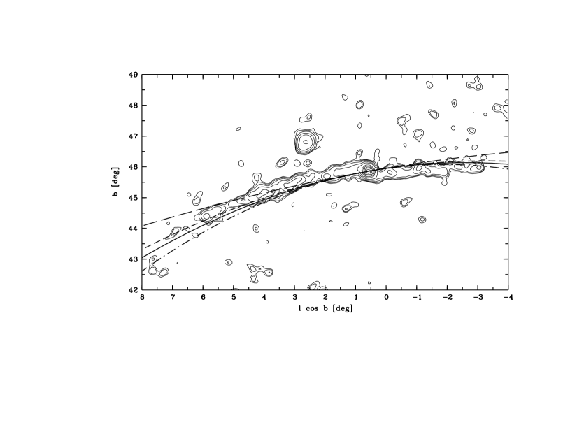
Figure 9: The tails and the local Galactic orbit of Pal 5 plotted in galactic coordinates $l\cos b,b$. Projections of four different orbits, all with tangent towards position angle $280^{\circ}$ at the center of the cluster, are overplotted on the contour map of Fig. 3. Long-dashed line: Straight line (i.e., unaccelerated) motion. Solid line: Locally best-fitting orbit in a radial field of constant acceleration $a=(220\,\mbox{km\,s${}^{-1}$})^{2}/18.5\,\mathrm{kpc}$. Here, the cluster has a tangential velocity of $v_{t}=95$ km s^-1 (galactic rest frame, but viewed from the position of the Sun). Dashed and dashed-dotted lines: Orbits in the same field, but with $v_{t}=110$ km s^-1 and $v_{t}=80$ km s^-1, respectively. Note that a logarithmic potential with circular velocity $v_{c}=220$ km s^-1 instead of the $a=const$ field yields projected local orbits that are practically identical to those shown above.

First of all, this sets a tight constraint on the direction of the cluster’s velocity vector in the tangential plane. The tails imply that the tangential motion of the cluster has a position angle of $231^{\circ}\pm 2^{\circ}$ with respect to the direction pointing to the northern equatorial pole, and $280^{\circ}\pm 2^{\circ}$ with respect to Galactic North (see Fig. 8). The orientation of this angle (i.e., $PA=280^{\circ}$ and not $PA=100^{\circ}$) follows when taking into account the direction to the Galactic center. Figure 9 shows the surface density map of the tails on a grid of galactic celestial coordinates $l\cos b,b$, where $l$ means galactic longitude and $b$ galactic latitude. Since the Galactic center ($l=0,b=0$) lies to the bottom of this plot, the tail that points to the right (also called the southern tail), must be the one at smaller galactocentric distance, which is thus leading, and the tail that points to the left (also called northern tail) be the more distant one, which trails behind. This means that the cluster is in prograde rotation about the Galaxy, in agreement with indications from different measurements of its absolute proper motion (Schweitzer, Cudworth & Majewski 1993; Scholz et al. 1999; Cudworth 1998 unpublished, cited in Dinescu et al. 1999).

Next we consider whether the observed part of the stream is long enough to see a deviation from straight line motion. Figure 9 demonstrates that this curvature is indeed detectable. The long dashed line shows the projection of a straight line in space (with position angle $280^{\circ}$) plotted over the surface density contours of the debris. The curvature of this line (due to projection onto the $(l\cos b,b)$ coordinate grid) is obviously too small to fit the tidal stream. Thus the curvature of the stream provides clear, direct evidence that the motion of the cluster is accelerated.

To further constrain the orbit, the radial velocity of the cluster in the Galactic frame is needed and an assumption on the acceleration field near the cluster has to be made. The cluster’s heliocentric radial velocity of $-58.7\pm 0.2$ km s^-1 (Paper II), combined with a solar motion of $(U,V,W)_{\odot}=(10.0,5.3,7.2)$ km s^-1 (Dehnen & Binney 1998b, velocity components in our $x,y,z$ system), and $v_{\mathrm{LSR}}=220$ km s^-1 for the rotation velocity of the local standard of rest yields a Galactic rest frame radial velocity of $-44.3$ km s^-1(observer at rest at the present location of the Sun). The cluster’s absolute proper motion is not yet measured with comparable accuracy. However, the existing measurements (see the above references) can be used to derive rough limits for the tangential velocity. According to Cudworth’s measurement, which we consider to be the most reliable one, the absolute proper motion of Pal 5 lies between 2.6 and 3.8 mas/yr (3-$\sigma$ limits). Using the above values for the cluster’s distance and the motion of the Sun and assuming the direction of the tangential velocity to be near $PA=280^{\circ}$, this yields a lower and upper limit for $v_{t}$ (i.e., tangential velocity as seen by observer at rest at present location of the Sun) of 60 km s^-1 and 195 km s^-1, respectively. To determine possible space velocity vectors for the cluster we thus combined the radial velocity with tangential velocities in the range from 50 km s^-1 to 200 km s^-1and the direction $PA=280^{\circ}$.

The simplest way to model the local acceleration field near the position of the cluster is a spherically symmetric field with constant acceleration. Assuming that the circular velocity in the Galactic halo is between 150 km s^-1 and 250 km s^-1, it follows that plausible values for the acceleration $a$ range from $(150\,\mbox{km\,s${}^{-1}$})^{2}/R_{cl}$ to $(250\,\mbox{km\,s${}^{-1}$})^{2}/R_{cl}$, with $R_{cl}$ being the cluster’s galactocentric distance. We thus adopted $a=(220\,\mbox{km\,s${}^{-1}$})^{2}/18.5\,\mathrm{kpc}$ and used this to integrate the orbit locally for a sequence of tangential velocities covering the interval from 40 to 180 km s^-1 in steps of 5 to 10 km s^-1. Each orbit (more precisely its projection on the plane of the sky) was then compared with the tidal tails. It turned out that an orbit with a good fit to the geometry of the tails is obtained when using $v_{t}=95\,\mbox{km\,s${}^{-1}$}$. This orbit is shown by the solid line in Figure 9. Changing $v_{t}$ by $\pm 15\,\mbox{km\,s${}^{-1}$}$ leads to orbits with significantly different curvature (short-dashed and dot-dashed line in Fig. 9) which fit the tidal tails less well. These cases are considered as the limits of the range of acceptable orbits. For other values of $a$ in the above range one can obtain orbits with essentially the same projected path when increasing or decreasing $v_{t}$ accordingly. This means that fitting a local orbit to the tidal tails sets up a relation between the acceleration $a$ and the cluster’s tangential velocity $v_{t}$. The value of $a$ can however not be determined in this way from the current data unless the velocity $v_{t}$ is known independently.

A more realistic model for the Galactic field near the cluster is given by the spherical logarithmic potential $\Phi=v_{c}^{2}\ln R$, which yields a constant circular velocity $v_{c}$ rather than constant acceleration. We repeated the orbit integration using this model and again looked for the best accordance with the geometry of the tidal tails. It turns out that for similar sets of parameter values the orbits obtained with this potential have practically the same projected paths as those obtained with the $a=const$ model. This implies that local variations in the size of the acceleration vector have little influence on the determination of the cluster’s local orbit. Hence it does not matter which of the two models we use.

The relation between the circular velocity $v_{c}$ of the logarithmic potential (or the local acceleration $a=v+c^{2}/18.5$ kpc) and the tangential velocity $v_{t}$ of the cluster, for which one obtains a local orbit with a projected path identical to the solid line in Figure 9, is shown in Figure 10. This relation is linear with a slope $dv_{t}/dv_{c}=0.43$. A straightforward way to determine the parameter $v_{c}$ of the potential would be to obtain $v_{t}$ through a precise astrometric measurement of the cluster’s absolute proper motion. An accuracy of 5 km s^-1 in $v_{c}$ would require an accuracy of 2 km s^-1 in $v_{t}$, which at $d=23.2$ kpc corresponds to a proper motion error of 18 $\mu$as/y. This level of accuracy can be achieved in future astrometric space missions like SIM and GAIA . On the other hand, from the currently available proper motion measurements for Pal 5 one can clearly not derive a meaningful constraint on $v_{c}$. The proper motion obtained by Cudworth yields $v_{t}=135$ km s^-1and would thus suggest $v_{c}>300$ km s^-1, which is uncomfortably high. The quoted error of this proper motion of 0.17 mas/y per component results in a typical uncertainty of 19 km s^-1 in $v_{t}$, so that $v_{c}$ cannot be determined to better than $\pm$47 km s^-1 from this data. A more comprehensive way of constraining the Galactic potential however consists in gathering kinematic data all along the tails and not only for the cluster. This will allow to use more complex models for the potential and to determine more than one parameter (e.g., the size and the direction of the local acceleration vector).

In spherical potentials, the simplest motion would be that on a circular orbit. However, there is no such solution in the above sequence of orbits because for the given position, radial velocity, and direction of tangential motion a circular orbit would require a tangential velocity of $v_{t}=885.5\,\mbox{km\,s${}^{-1}$}$, the total velocity on this orbit then being $v_{c}=886.6\,\mbox{km\,s${}^{-1}$}$. Apart from the fact that velocities of this size are very far from realistic, it turns out that the projection of the resulting orbit would be similar to that of motion on a straight line (see Fig.9) and hence not yield a good fit to the tidal tails. In order to allow a circular orbit with a velocity of 220 km s^-1 or less one needs to increase the position angle of the tangential velocity to $PA\geq 310^{\circ}$. However, the orbit would then deviate from the direction of the tails by at least $30^{\circ}$. A circular or nearly circular orbit is thus not an option.

We also checked for possible effects from a flattening of the Galactic potential. The potential in the Galactic halo is in fact likely to be flattened because of the influence of the disk, and may have additional flattening due to a flattened distribution of mass in the halo. We thus constructed a model composed of (a) an exponential disk with scale length $h_{r}=3\,\mathrm{kpc}$, scale height $h_{z}=0.3\,\mathrm{kpc}$, and mass density $0.12\,M_{\odot}\mathrm{pc}^{-3}$ near the solar circle, and (b) a modified logarithmic halo potential $\Phi_{h}=v_{c}^{2}\ln((r^{2}+(z/q)^{2})^{1/2})$ with $v_{c}=180\,\mbox{km\,s${}^{-1}$}$. Here, $r=(x^{2}+y^{2})^{-1/2}$ denotes the cylindrical radius. Together, the two components yield a flat rotation curve (in the Galactic plane) with a velocity of about 220 km s^-1. In the region near the cluster the contribution of the disk to the total potential can be described with only a monopole and a quadrupole term. For the halo component two cases were considered, a spherical halo ($q=1.0$) and a flattened halo with $q=0.8$. Again, we find that these potentials lead to orbits whose local projections are practically indistiguishable from those obtained with the previous models. For $q=1.0$ the best-fit projected local orbit (in the sense of the solid line in Figure 9) requires $v_{t}=90\,\mbox{km\,s${}^{-1}$}$. In the case of $q=0.8$ an equivalent orbit, i.e., with the same local projected path, can be obtained by increasing the tangential velocity to $v_{t}=105\,\mbox{km\,s${}^{-1}$}$. This demonstrates that over the currently known angular extent of the tidal tails the projected orbital path of the cluster is not sensitive to the flattening of the Galactic potential.

In conclusion, the fit of the cluster’s projected orbital path to the geometry of the tidal tails does not depend on a particular model for the Galactic field. As long as there are no additional kinematic constraints from radial velocities or proper motions along the tails the result of the fit is compatible with a variety of orbits for different fields, which locally project onto the same path on the sky. Those orbits of course differ from each other along the line-of-sight. However, within the region where we see the tidal tails the differences are not substantial. This allows us to estimate how much the distance varies along the cluster’s orbit over the $10^{\circ}$ arc of the stream. It turns out that the end of the leading tail at $l\cos b=-3\fdg 2$ lies nearest to the observer, in accordance with the negative radial velocity of the cluster. The different orbits obtained with the above selection of Galactic models put this point at a galactocentric distance $R$ between 17.6 and 17.9 kpc, and at a heliocentric distance $d$ of 22.1 to 22.4 kpc. For the opposite end of the trailing tail at $l\cos b=+7\fdg 0$ these orbits predict galactocentric distances between 18.6 and 19.0 kpc, and heliocentric distances of 23.4 to 23.9 kpc. The maximum of $d$ lies between 23.6 and 23.9 kpc. The distance between the cluster’s orbit and the observer thus varies by up to 1.8 kpc over the length of both tails. This is a variation of +3% and $-$5% relative to the present distance of the cluster. Observationally, this corresponds to a magnitude difference of +0.06 mag and $-$0.1 mag, respectively, which is completely consistent with the results presented in §4.4.

The maximum value of $R$ along the local orbit lies in the range from 18.7 to 19.4 kpc (see upper panel of Fig.10). All solutions for the local orbit place its apocenter between 4$\fdg$1 and 6$\fdg$6 in $l\cos b$. This reveals that the cluster’s present position must be close to the apocenter of its orbit. The different orbit solutions suggest that the cluster passed this apogalactic point between 13 and 27 Myrs ago. The cluster’s proximity to an apogalactic point implies, that the variation of the galactocentric distance $R$ along the local orbit is small. Indeed, in the region of the trailing tail the variation of R along the orbit is at most 0.6 kpc or 3%, and in the region of the leading tail this variation is 0.9 kpc or 5% (see the above minimum and maximum values).

5.3 Is the tail aligned with the orbit?

With a model of the cluster’s orbit at hand, we can a posteriori test and validate our working hypothesis that the tidal tails lie parallel to the local orbital path of the cluster even if the stars do not have exactly the same velocity as the cluster when they decouple from the cluster. To this end we simulated a sample of test particles in a spherical logarithmic potential with $v_{c}=220$ km s^-1. The particles were released over the time interval from $-$2.0 Gyr to present at equal time steps of 20 Myr. We emphasize that this experiment is not meant to provide a realistic model of the mass loss history of the cluster, but just serves to reveal the geometry of the tails. The particles were released from the cluster with a radial offset, i.e., either in the direction of the Galactic center or in the opposite direction, and with small velocity offsets. The size of the radial offset was chosen to be $3\times r_{L}$, with $r_{L}$ the distance of the Lagrange point of local force balance between the cluster and the Galactic potential, i.e.,

$$r_{L}^{3}=GM_{cl}\frac{R^{2}}{v_{c}^{2}}$$ (8)

For the present position of the cluster equation (8) yields $r_{L}=57$ pc, using $M_{cl}=6\times 10^{3}M_{\odot}$ as the mass of the cluster. The velocities of the particles were offset from the velocity of the cluster by a velocity vector with a size of 1.0 km s^-1 (i.e., about $2\times$ the dynamical velocity dispersion of the cluster, see Paper II), pointing either in the radial direction (i.e., towards the Galactic center on the inner side and away from it on the outer side) or at $45^{\circ}$ from this direction.

Figure 11 shows the distribution of this sample of test particles in the plane of the sky at $t=0$. The plot covers the same field as Figure 9 and uses the same (galactic) coordinates. The solid line shows the path of the cluster’s orbit, same as in Figure 9. It can be seen that the stream of test particles has approximately the same width as the observed tails, and that it is well aligned to the cluster’s projected orbital path. In other words, the relatively small peculiar velocities that stars may have when escaping from Pal 5 do not have a significant impact on the mean location of the tidal debris with respect to the cluster’s orbit, at least not in projection onto the plane of the sky. Thus our assumption, that the orbit of the cluster must be fit such that it is parallel to the observed tidal tails proves to be entirely valid.

5.4 Global orbit

We saw that the apogalactic distance $R_{max}$ of Pal 5 can be derived from the local orbit and hence does not strongly depend on specific assumptions on the Galactic field. However, the determination of other characteristic parameters of the cluster’s orbit such as the perigalactic distance $R_{min}$ or the distance $R(z=0)$ at which the cluster crosses the Galactic disk requires extensive extrapolation beyond the region of the tails and thus depends on a global Galactic mass model. In order to estimate these and other orbital parameters we made use of Model 2 from the series of Galactic models developed by Dehnen & Binney (1998a). This mass model consists of three exponential disks representing the stellar thin and thick disk and the interstellar material, and of a bulge and a halo component. The parameters of the model are chosen such that the model accomodates a variety of observational constraints, e.g., the Milky Way’s rotation curve, the local vertical force, the local surface density of the disk etc. (for details see Dehnen & Binney 1998a).

The tangential velocity of Pal 5 was set to $v_{t}=90$ km s^-1. Hereby the above model provides an orbit whose path locally coincides with the solid line in Figure 9 and hence meets the condition of a good fit to the tidal tails . The equations of motion were integrated over the time interval from $-$1 Gyr to 1 Gyr. Part of the resulting orbit is shown in Figure 12abc. We find that the orbit has perigalactic distances in the range from 6.7 to 5.7 kpc. This reveals that the cluster penetrates deeply into the inner part of the Milky Way. The typical time scales of the orbit are $<T_{R}>=291$ Myr (mean period of radial oscillation) and $<T_{\psi}>=443$ Myr (mean period of rotation around the Galactic z-axis). The local constraints from the tidal tails allow us to vary $v_{t}$ by about $\pm 10$ km s^-1. When doing so the perigalactic distances of the orbit change by about $\pm 0.8$ kpc, and the eccentricity thus varies by $\pm 0.05$. The periods $<T_{R}>$ and $<T_{\psi}>$ change only slightly, i.e., by $\pm 3\%$ and $\pm 1\%$.

From $-$1 Gyr to present the orbit makes five disk crossings. Three of them happen near or inside the solar circle, at distances of 6.7, 6.8, and 8.3 kpc, while two are at much larger distances of 14 to 18 kpc. When changing $v_{t}$ by $\pm 10$ km s^-1 the galactocentric distances of the crossings of the inner disk vary by typically $\pm 0.7$ kpc but occasionally up to $\pm 1.1$ kpc. Interestingly, the predicted location of the next future disk crossing is at an even lower galactocentric distance of $5.9\pm 0.8$ kpc, which is very close to the next perigalacticon (see Figs.12a and 12b). This disk crossing is predicted to happen in $+110\pm 2$ Myr from present.

Besides the models of Dehnen & Binney there exist a variety of other Milky Way mass models from other authors, e.g., Pacynski (1990), Allen & Santillan (1991), Johnston et al. (1995), Flynn et al. (1996). To test in how far our conclusions on the orbit of Pal 5 depend on the particular model we repeated the integration of the orbit using the same initial velocities and the Milky Way mass model of Allen & Santillan. This is a three-component model with bulge, disk, and halo, where the disk potential is of the Miyamoto-Nagai form (Miyamoto & Nagai 1975). The corresponding orbit is shown in Figure 12def. The general characteristics of the orbit are very similar to the one found with the Dehnen & Binney potential. In particular, we find small pericentric distances down to 5.5 kpc. This confirms that the orbit of the cluster leads through the inner part of the Milky Way. The sequence of near and far disk crossings and apogalactic and perigalactic passages is the same as with the other model, but the associated time scales are somewhat shorter (e.g., $<T_{R}>=275$ Myr, $<T_{\psi}>=412$ Myr). Again, the orbit predicts an exceptionally small galactocentric distance, namely of 5.7 kpc for the next crossing of the disk (in about 107 Myrs from present). When using a simple spherical logarithmic potential with $v_{c}$ in the range from 150 to 260 km s^-1 the resulting orbits yield even lower values for the galactocentric distance of this disk passage. It thus appears that an upper distance limit of $R\leq 6$ kpc for the next disk crossing is a safe prediction.

6 Clues on the mass loss history

6.1 Mean mass loss rate

Using the results from §5 we can translate the amount of mass that is observed in the tails of Pal 5 into a rough estimate of the mean mass loss rate. It was shown that the variation of $R$ along the local orbit is small, in particular in the region of the trailing tail. This means that the variation of the angular velocity $\dot{\varphi}=L/R^{2}$ along the local orbit is also small. Assuming $L=const$, the relative change in $\dot{\varphi}$ is twice the relative change in $R$ and thus $\leq 6\%$ for the trailing tail and $\leq 10\%$ for the leading tail. Therefore, it is justified to estimate the time scale of the angular drift between the debris and the cluster in the way described by equation (7).

The key parameter is the relative radial offset $\alpha$ from the orbit of the cluster. In reality, individual stars do not escape from the cluster under exactly the same conditions and hence do not settle on orbits with the same radial offset. Their orbits will not even be strictly confocal because they do not escape with exactly the same velocity. Hence stars at a certain azimuthal distance from the cluster will have taken different intervals of time to drift to this place. However we assume, that we can estimate the mean time scale $\Delta t$ of this drift by applying equation (7) to the mean value of $\alpha$.

To determine the mean offset we measured for each star its rectangular separation from the solid line of Figure 9 in the plane of the sky. We then counted the weighted number of stars in $2^{\prime}$ wide bins of this rectangular separation, using the same weighting scheme as described in §3.2. Separate counts were made for the leading and the trailing tail. The resulting star count histograms are plotted in Figure 13. Each tail shows up as a symmetric peak on top of a constant background. We determined the center and the width of each peak by fitting a Gaussian plus a constant to the counts (see dashed lines in Fig. 13). For the trailing tail we thus measure a mean rectangular separation of 11$\farcm$8$\pm$0$\farcm$5 from the orbit and a FWHM of 18$\farcm$4$\pm$1$\farcm$2. For the leading tail we find a mean separation of 10$\farcm$1$\pm$0$\farcm$8 and a FWHM of 17$\farcm$2$\pm$1$\farcm$9. From the mean angular separations as seen in projection we reconstructed the mean radial distance between the debris and the orbit of the cluster in the orbital plane. This was done in the following way: We increased and decreased the length of the galactocentric radius vector of the cluster by 200 pc, determined the positions of the endpoints of these vectors on the sky as observed from the Sun, and then computed the rectangular separation of these points from the projected orbit in the same way as done for the stars. This yields separations of 9$\farcm$0 and 9$\farcm$1, respectively, i.e., 0.76 and 0.90 times the observed separations. This implies that the observed separations correspond to mean radial distances between the tails and the orbit of 263 pc for the trailing tail and 222 pc for the leading tail.

We first focus on the trailing tail, which is better covered by the observations and which is most suited for applying equation (7). Using $v_{t}=95$ km s^-1 the angular momentum of the cluster’s orbit is $L=1814$ km s^-1 kpc . From $R_{max}=19.0$ kpc we derive the angular velocity at the apogalactic point as $\dot{\varphi}=5.14$ km s^-1/kpc or, in other units, $\dot{\varphi}=0\fdg 295$/Myr. Comparing the mean radial offset of the tail of 263 pc and the apogalactic distance of 19.0 kpc we have $\alpha=1.014$. The material in the trailing tail is basically spread over an arc of $6^{\circ}$ on the sky. Along this arc, the orbit of the cluster subtends an azimuth angle of 7$\fdg$7 in the orbital plane.

Putting these numbers into equation (7) we obtain $\Delta t=1.94$ Gyr. This is the typical time it has taken debris stars to drift from the cluster center to the “tip” of the tail. The trailing tail contains about 0.8 times as many stars as the cluster (see §4.1). If we assume that the tail has the same mass function as the cluster, the mass in the tail should be $0.8\times M_{cl}$, where $M_{cl}$ denotes the present mass of the cluster. With regard to the mass function, this is a lower limit, because the tail is likely to contain a larger fraction of low-mass stars than the cluster. The cluster is known to be underabundant in low-mass stars and may have lost them through mass segregation followed by tidal stripping from the outer part of the cluster. Since low-mass stars are not represented in our sample such a difference in the mass function would result in a somewhat higher total mass of the tail. Using the above values, and taking into account that equal amounts of mass are lost on both sides of the cluster, we finally obtain an estimate of the mean mass loss rate of $-\dot{M}/M_{cl}=0.82$/Gyr. Multiplying by the present mass of the cluster, which has recently been estimated to be $-M_{cl}=6\times 10^{3}M_{\odot}$ (Paper II), we get $\dot{M}=4.9M_{\odot}$/Myr.

To check this result we do an analogous calculation for the leading tail using a mean distance of $R=18.2$ kpc (see §5.2). The mean angular velocity then is $\dot{\varphi}=0.321^{\circ}$/Myr, and the mean radial offset of the tail from the orbit of the cluster yields $\alpha=0.988$. Furthermore we have $\delta\varphi=4\fdg 8$ as the azimuth angle of the orbit along the leading tail (seen from the Galactic center), and $M_{tail}=0.4M_{cl}$ as an estimate of its mass (see §4.1). Equation (7) thus yields $\Delta t=1.26$ Gyr, and this leads to a mean mass loss rate of $-\dot{M}/M_{cl}=0.63$/Gyr or $-\dot{M}=3.8M_{\odot}$/Myr. This rate is somewhat lower than the one obtained from the trailing tail because the mean drift rate along the leading tail is only slightly higher and cannot compensate the lower surface density in the leading tail.

The accuracy of these estimates is limited by a number of potential sources of errors, the most important of which are: (1) The uncertainty in the determination of the offset between the tails and the orbit. (2) The uncertainty of the angular velocity resulting from errors in the distance and the tangential velocity of the cluster. (3) Deviations of the motion of individual stars from the drift rate at the mean radial offset due to a spread in their initial positions and velocities. While the fitting of the histograms of Figure 13 yields a formal uncertainties of 0$\farcm$5 and 0$\farcm$8 for the mean angular separation, we expect that the true error of this quantity is more like $1^{\prime}$ to 1$\farcm$5, in particular because the exact location of the cluster’s orbit is not known. The relative error in the mean angular separation and hence in the mean radial offset is thus assumed to be between 10% and 15%, producing a relative error in the factor $(\alpha-1)/\alpha$ of approximately the same size. The heliocentric distance and the estimate of the tangential velocity of the cluster are both thought to have a relative uncertainty of 10%. This translates into relative errors of 12% and 10% for the corresponding galactocentric quantities and thus results in a combined error for the angular velocity $\dot{\varphi}$ of 16%. Hereby, the relative error in the fractional mass loss rate would be about 22%. How much the above estimate of the mass loss rate is biassed by the spread in the drift motions of individual stars needs to be investigated with forthcoming detailed N-body simulations of the tidal disruption Pal 5. However, we expect that this may also contribute a relative uncertainty of about 20%. The total error is thus believed to be of the order of 30%. In conclusion, our result for the mean mass loss rate of the cluster with respect to its present mass is $-\dot{M}/M_{cl}=0.7\pm 0.2$/Gyr or $-\dot{M}=4.3\pm 1.3M_{\odot}$/Myr (average from both tails).

It is interesting to compare this mass loss rate with predictions from approximate formulae devised by Johnston et al. 2002 (hereafter JCG02) for calculating mass loss rates of satellites from radial surface density profiles. These formulae (see equations (6) and (7) of JCG02) relate the mass loss rate to the break radius of the surface density profile, the surface density outside this radius, and the time period for orbital or circular motion, assuming that the radial profile decreases as either $r^{-1}$ or $r^{-2}$. Since the observed profiles for Pal5 are characterized by $-1.5\leq\gamma\leq-1.2$ they lie in between those two cases. We calculated the predicted mass loss rates with two different radii, $r=20^{\prime}$ and $r=60^{\prime}$. Using $r_{break}=16^{\prime}$, average surface densities as provided in Figure 5, and the time scales $T_{orb}=356$ Myr, $T_{circ}=528$ Myr, equation (6) of JCG02 predicts mass loss rates of $6.2M_{\odot}$/Myr ($withr=20^{\prime}$) and $3.7M_{\odot}$/Myr (with $r=60^{\prime}$) while equation (7) of JCG02 predicts mass loss rates of $2.1M_{\odot}$/Myr and $3.8M_{\odot}$/Myr, respectively. The predictions are hence within 50% of our above detailed estimate of the mean mass loss rate of the cluster.

6.2 Total mass loss

According to numerical simulations the mean rate of tidal mass loss of a globular cluster orbiting in a stationary Galactic potential remains approximately constant over most of its lifetime, i.e., the cluster’s mass decreases approximately linear with time (see, e.g., Gnedin et al.  1999, Johnston et al. 1999a, Baumgardt & Makino 2002). From the observations it is not entirely clear whether this really holds for Pal 5 because the outward decrease of the linear density of the tails could be interpreted as an indication for a secular increase in the mean mass loss with time. However, if we assume that the mean mass loss rate was constant, we can use the measured mean rate of recent mass loss to get an idea of the cluster’s mass at earlier epochs. An important condition is that the Galactic potential must have been essentially the same over the time interval spanned by the extrapolation. Extrapolating over the cluster’s entire age of 12 Gyr thus poses a problem because disk shocks seem to be an important driver of the mass loss of Pal 5, and the age distribution of disk stars suggests that the Galactic disk was not in place at very early epochs. However, if the disk was less massive or non-existent early on, the initial rate of the cluster’s tidal mass loss was presumably lower than the present rate. Therefore, an extrapolation with the present mass loss rate may overestimate the cluster’s initial mass but can put an upper limit on it.

Our measurements suggest a mean mass loss rate of $-\dot{M}/M_{cl}=0.7$/Gyr. Multiplying this with 12 Gyr and adding the cluster’s present mass, we obtain an upper limit for the cluster’s initial mass of $M=9.4M_{cl}$. Pal 5 may thus have started with roughly ten times as much mass as it has today. If one restricts the extrapolation to a time interval of about 8 Gyr, for which the existence of a massive Galactic disk is likely, one obtains a cluster mass of $6.6M_{cl}$. Since the cluster is certainly older than 8 Gyr, this presents a lower limit to its initial mass, provided that the cluster has been on its present orbit during the entire period. Of course, these limits vary as a function of the error of the mass loss rate and provide not more than a rough guide line.

7 Discussion and Summary

7.1 Compelling evidence for tidal disruption

Our analysis of an enlarged set of SDSS data reveals that the cluster Pal 5 is connected to a long stream of tidal debris that contains at least 1.2 times as much stellar mass as the cluster itself contains in its present state. This confirms and extends the results of Paper I, which presented first evidence for tidal tails from a study of a smaller field. The most basic aspect of these results is that they provide the first stringent observational proof that globular clusters in the Milky Way’s halo may be subject to significant tidal mass loss, by which they eventually dissolve. The detection of fully-fledged tidal tails, which is unique so far, makes Pal 5 the prototype of such tidally-disrupting globular clusters. We showed that the stream of debris is thin and maintains its small width over a length of several kiloparsecs, suggesting that it is a kinematically cold system. This is very much consistent the low velocity dispersion inside the cluster, which is only about 0.5 km s^-1 (Paper II). The numerical experiment described in §5.3 and Figure 11 lends further support to this view. It is obvious that the relatively small transverse spread of the debris on the sky has strongly favored the detection of the stream. In the case of a massive cluster, having a much higher internal velocity dispersion, the debris would probably spread out in a much wider stream and thus be more difficult to detect. Another favorable circumstance is the fact that Pal 5 is presently located close to its apogalacticon. This means that the distribution of the debris has the smallest possible angular dispersion along the orbit and therefore shows a relatively high density.

7.2 The tails and the orbit of the cluster

It was demonstrated that the arc over which the tidal debris has been traced is now sufficiently long to recognize the intrinsic curvature of the stream. Since there is very good reason to assume that the tails are closely aligned with the orbit of the cluster the curvature of the stream reveals the local curvature of the cluster’s orbit. This is a remarkable point because curvature means acceleration. Direct measurements of the Galactic gravitational acceleration of an individual halo star or star cluster in the sense of observing a non-linear change in position or a change in velocity over time are for technical reasons totally out of reach. Therefore the curvature, and also the bipolar and S-shaped structure of Pal 5’s stream of debris provides one of the first occasions where the acceleration of a halo object by the gravitational field of the Galaxy is directly visible. A considerable drawback however is that the tidal stream is known only in projection on the plane of the sky. This projected view provides clear evidence that the acceleration of the cluster is non-zero, but does not yet allow to derive a useful constraint on its specific value. To achieve this the observations would need to cover a major part of the cluster’s orbit or one would require precise information on the tangential velocity of the cluster or on the variation of the distance or the kinematics along the tails. As an example, we determined the best-fitting orbits in a spherical logarithmic potential and showed that measuring the absolute proper motion of the cluster on the accuracy level of 10 $\mu$as/y would allow to estimate the local circular velocity to about 2%. This is similar to the conclusion drawn by Johnston et al. (1999b) from a study of simulated tidal streams.

Using different Galactic models and selecting orbits that optimally fit the tidal tails, we found that the cluster must be near its local maximum distance from the Galactic center and that therefore, the galactocentric as well as the heliocentric distance along its orbit varies by no more than a few percent over the length of the tails. This is in full agreement with the photometry, because color-magnitude diagrams show that there is no systematic difference in apparent brightness between the tidal debris and the cluster of more than 0.1 mag. On the other hand, it turned out that the pericenters of the cluster’s orbit must lie in the inner Galaxy, namely at $R\leq 7$ kpc. This means that its orbit is rather eccentric and that the cluster must have repeatedly crossed the Galactic disk near or inside the solar circle. Since such disk crossings at small galactocentric radii lead to strong tidal shocks this provides a convincing explanation for Pal 5’s heavy mass loss.

Of particular interest is the fact that the next disk crossing, which will happen in about 100 Myr, is predicted to take place at a galactocentric distance $\leq 6$ kpc, causing a very strong tidal shock. Given the small amount of mass that is left in the cluster and its low spatial concentration, one must suspect that this event will trigger the total disruption of the cluster. Dinescu et al. (1999), using formulae for the destruction rates due to disk- and bulge shocks as developed by Gnedin & Ostriker (1997) and orbital parameters determined from measured proper motions, derived a theoretical estimate of the destruction time of 0.1 Gyr for Pal 5. This is identical to our estimate for the time until the next disk crossing. On the other hand, the original paper by Gnedin & Ostriker (1997) gave estimates of the destruction time for Pal 5 of either 1.1 Gyr or 46 Gyr, depending on the model for the Galactic potential. These time scales are too long in view of what is known about Pal 5 now, and must have resulted from a very different model for the cluster’s orbit. This demonstrates the importance of reliable individual orbital data for clusters like Pal 5 since such data can place much stronger constraints on the dynamical evolution of these systems than purely theoretical analyses.

7.3 The surface density in the tails

The surface density distribution of the stars in the tails shows some important peculiarities:
(1) The distribution is clumpy, i.e., there are a number of density maxima and minima in each tail. While the density variations in the leading tail are moderate and not necessarily significant (i.e., they could still be the result of statistical fluctuations) the trailing tail shows at least two strong density maxima and one gap, where the local density deviates significantly from the mean density level. Although disk shocks, which are believed to be the primary cause of Pal 5’s mass loss, are likely to modulate the instantaneous mass loss rate, it is implausible that the observed clumps are due to this modulation because the density variations would then need to occur symmetrically in both tails. Also, such variations should preferentially be visible near the cluster while at larger angular distances they should be washed out by the differential drift between stars of different orbital energy.

The region of maximal stellar density in the trailing tail lies at arc lengths between 2$\fdg$3 and 3$\fdg$7 from the center of Pal 5. According to the results from §6.1 the mean rate of apparent drift of the tidal debris is 0$\fdg$31/100 Myr. Thus the stars that form this broad density clump are expected to have escaped from the cluster in the interval between 740 and 1190 Myr ago. In §5.4 we found that during the last 1 Gyr the cluster crossed the Galactic disk five times, and three times thereof at small distances from the Galactic center. The latter occurred 140 Myr, 480 Myr, and 740 Myr before present. If these inner disk crossings produce overdensities that can be observed as distinct clumps in projection on the sky, then one would expect to see one such clump close to the cluster ($\lambda\approx 0\fdg 3$) and two clumps - or perhaps one broad clump from the merging of the two - at arc lengths between 1$\fdg$5 and 2$\fdg$3. This does not correspond to the observations. In order to achieve some kind of agreement one would need to assume that the drift of the debris is in fact 50% faster than derived from the radial offset between the tails and the orbit of the cluster.

It may seem intriguing that the major density enhancement in the stream is near the apogalactic point of the cluster’s orbit. Nevertheless, the fact that a stellar stream gets compressed near the apocenter (because the angular velocity is minimal at this point) cannot explain this local enhancement because the angular scale of the observed feature (less than 2$\fdg$5 when viewed from the galactic center) is much too small. One could speculate that the density variations in the tails might come from scattering by small-scale perturbations of the Galactic potential as produced by spiral arms, molecular clouds, dark matter clumps etc. However it has not yet been demonstrated that such perturbations can indeed generate the observed features. We note that such perturbations would certainly need to be much weaker than those in a dark halo of massive ($\approx 10^{5}M_{\odot}$) black holes because encounters with such massive compact objects would have destroyed the cluster - and most likely also its tails - on a very short time scale (Moore 1993).

One might also think that the broad density enhancement in the trailing tail could be related to the cluster M 5 since it is uncomfortably close to it on the sky. But a dedicated search for debris from M 5 (using a proper color-magnitude filter for this cluster) yields absolutely no evidence for an extended distribution of M 5 stars that could overlap with the tail of Pal 5.

(2) Apart from local variations, the radial profile of the stellar surface density at $r\leq 20^{\prime}$ declines like a power law with an exponent of $-$1.2 to $-$1.5, which means that the linear density along the tails decreases slowly with increasing distance from the cluster. How does this compare to the results of N-body simulations of stellar systems in Milky Way like potentials? Combes et al. (1999) show density profiles for two of their simulated clusters and find that at radii $r>r_{t}$ the volume density of debris stars decreases like $r^{-4}$, hence the surface density decreases like $r^{-3}$. This is clearly a much steeper decline than the one we observe. In contrast to this Johnston et al. (1999a) show surface density profiles of simulated globular cluster-like systems, in which the unbound outer part has a much shallower decline that is almost like $1/r$. As these authors point out, such a $1/r$ decline can easily be explained if one considers the very simplified case of a cluster on a circular orbit, which looses mass at a constant rate and with constant energy offsets. Our observations are not extremely far from the simple $1/r$ case but do not match it exactly. More recently Johnston et al. (2002), presented a series of simulations, in which the obtained radial surface density profiles that show a wide variety of logarithmic slopes in the outer part. They report values for the power-law exponent $\gamma$ between $-$1 and $-$4, and show that the result depends to some extent on the parameters of the orbit and the orbital phase. Even for an almost circular orbit they find $\gamma$ to scatter between $-$1 and $-$3. For very eccentric orbits their simulations seem to predict that $\gamma$ is mostly below $-3$, in particular at the apocenter. However, the system parameters (mass,radius) and the orbits that were used in these recent simulations are actually more representative of dwarf satellites than of clusters like Pal 5. The conclusion from this comparison is that different simulations predict a wide range of possible power law exponents for the debris and that our observed values of $\gamma$ lie in the upper part of this range.

The fact that in both tails the observed surface density profile is somewhat steeper than the simple $1/r$ may indicate that either the angular velocity along the orbit increases with increasing angular distance from the cluster or the (orbit-averaged) mass loss rate has undergone a secular change. The variation of the orbital angular velocity must certainly enter the game on larger scales but cannot have a significant impact on the present results because the arc length of the tails is too short. We are thus left with the possibility that the mean mass loss rate may have steadily increased or that the mass loss process may have suddenly set in not much longer than 2 Gyrs ago. In the latter case an outward decrease of the linear density of the tails could result from the fact that the tip of each tail would only contain stars with the highest energy offset from the cluster, which should occur in low numbers, while at smaller angular distance from the cluster one would find both, stars with smaller energy offset, which should be more numerous, and also stars with higher energy offset, which were released from the cluster more recently.

Indeed, the traces of the trailing tail disappear before the tail would reach the edge of the observed field, and it is unknown whether or not the stream continues and reappears with significant density farther out along the orbit. If so, there would be a gap or a section of very low density with an arc length $\leq 1^{\circ}$, that would need to be explained. If not, this would imply that the mass loss history of Pal 5 underwent an abrupt change about 2 Gyr ago and that the mass loss rate in the earlier phase was much lower than in the recent phase or even zero. This would certainly require a fundamental change of the cluster’s orbit.

One possibility would then be that Pal 5 came from outside the Galaxy and was accreted by it in a merger event with a smaller galaxy. This merger event would need to have happened fairly recently, and the cluster would have been accreted as a system with a mass of only $1.5\times 10^{4}M_{\odot}$. As we will discuss in §7.7, an association of Pal 5 with the Sagittarius (Sgr) dSph galaxy is very unlikely. From statistical studies there is evidence for further halo substructure, i.e., possible great circle streams of outer halo satellites (e.g., Lynden-Bell & Lynden-Bell 1995, Palma et al. 2002), which might be a hint on former merger events. However, based on sky position, distance, and radial velocity, Pal 5 has not qualified as a possible member of any hypothetical stream in these studies. Since not all of the satellites may in fact belong to such a stream, an association with an individual satellite needs not necessarily be obvious through great circle alignments. In this sense the question of whether or not Pal 5 is likely to be associated with one of the dSph satellites remains open because there is currently no well-constrained orbital information on most of these objects.

As another possibility we mention that the orbit of Pal 5 could have changed drastically through a close encounter with one of the Milky Way satellites. Since the present orbit of Pal 5 is unlikely to reach beyond galactocentric distances of 20 kpc, the only known candidate for such an encounter would be the Sgr dwarf spheroidal. However such scenarios are highly speculative. It is thus very important to learn more about the spatial extent of the stream.

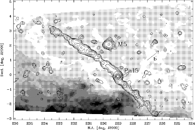
Figure 14: Grey-scale map of interstellar extinction in the $g$ band based on the reddening data of Schlegel, Finkbeiner & Davis (1998). The different grey scales represent extinction values $A_{g}$ from 0.15 mag (lightest grey) to 0.75 mag (black). Overlaid are the contours of the surface density of Pal 5 stars shown in Figure 3. The arrow labeled with $b$ indicates the direction of increasing galactic latitude.

(3) Overall, the stellar surface density in the leading tail is on a lower level than in the trailing tail. This is surprising because the symmetry of the tidal force field suggests that the distribution of tidal debris should - at least in the vicinity of the cluster - be symmetric with respect to the cluster center. Both, orbit calculations and the analysis of the photometric data have shown that variations in the line-of-sight distances cannot be responsible for this effect. One may thus wonder if the star count results could be influenced by variable interstellar extinction. In Figure 14 we show the surface density contours of Pal 5 and its tidal stream overplotted on a grey-scale map of interstellar extinction derived from the reddening data of Schlegel, Finkbeiner & Davis (1998). Although integrated Galactic foreground extinction corrections do not necessarily hold for stars within the Milky Way because they are integrated along the entire line of sight, we believe that this only leads to small errors for a cluster as distant and as far above the plane as Pal 5. Another possible effect is the dependence of extinction on stellar temperature (and thus color) as discussed in Grebel & Roberts (1995). Considering our filter choice and color range, this should amount to at most 0.02 to 0.03 mag uncertainty, which is negligible for our purposes.

Figure 14 reveals that there is indeed significant variation in interstellar extinction over the field, as was already mentioned in §2. One notices that the leading tail is located close to the region of enhanced extinction but fortunately does not run across this region. This shows that there is little reason to assume a significant impact of extinction on the measurement of the stellar surface density in the tails. If enhanced extinction played a role, it would result in a loss of faint stars close to the detection limit. While the definition of our sample already involves a magnitude cut-off at $i^{*}=21.8$ well above the limit, we tentatively increased the cut-off by an additional 0.5 mag, thus restricting the sample to $i\leq 21.3$. It turned out that the resulting surface density distribution is similar to the one for the larger sample and maintains the same overall imbalance between the leading and the trailing tail. It is therefore clear that the overall difference between the number counts in the two tails is not the result of variable extinction.

7.4 The luminosity functions

We showed that the luminosity function of the stars in the tidal tails is in very good agreement with the stellar luminosity function in the cluster. This result is not self-evident, although it nicely fits the idea that the tails consist of stars from the same stellar population as the cluster. As briefly noted in previous sections, a deep study of the core of Pal 5 using the HST (Grillmair & Smith 2001) has revealed that the luminosity function of Pal 5 is relatively flat. This means that there is a strong deficiency in low-mass stars, at least in the core of the cluster. If this deficiency is a consequence of tidal mass loss (in combination with mass segregation), as Grillmair & Smith suggested, one would expect to find a corresponding overabundance of low-mass stars in the cluster’s debris. The luminosity functions should then actually be different. However, the flattening of the luminosity function shown by Grillmair & Smith becomes effective at absolute magnitudes $M_{I}>5$ mag which is below the limit of our analysis of SDSS data. Therefore, even though we find that the luminosity functions of the tails and the cluster agree down to the limit of this study, it seems likely that they will diverge when probing the stellar content of the tails at fainter magnitudes. If so, the higher fraction of low-mass stars in the tidal debris will contribute additional mass to the tails. This means that our current estimate of the mass ratio between the tails and the cluster (§4.1) provides a lower limit while the true mass ratio may be somewhat higher.

7.5 The mass loss rate

We showed that the transverse offset between the tails and the cluster can be used to estimate the time needed by debris stars to drift away from the cluster by a certain angle. This leads to the conclusion that the tails in their currently known extent represent the cluster’s mass loss from essentially the last 2 Gyrs. The result of our numerical experiment on the drift of debris along the cluster’s orbit, which is shown in Figure 11, confirms this time scale. It follows that the mean mass loss rate of Pal 5 in this period was about 0.7($\pm$ 0.2) times the present mass of the cluster per Gyr. However, these estimates involve a number of approximations and simplifying assumptions. In particular, it remains to be investigated whether the fact that stars are actually distributed over a range of velocities and positions when escaping from the cluster leads to a substantial bias in the above estimates. For more definitive results accurate modelling of the details of the mass loss process are needed. Thus N-body simulations of the system under realistic conditions need to be performed.

A simple extrapolation with the present mean mass loss rate shows that the cluster may initially have had a total mass of between 6 and 10 times its present mass. Obviously, such an estimate depends on whether the cluster maintained the same mean (i.e., orbit-averaged) mass loss rate over most of its lifetime. For time intervals in which (1) the Galactic potential was the same as today and in which (2) the cluster followed the same orbit as it is today, one can indeed expect this to hold true. However, the observed decline of the surface density of the tails with increasing distance from the cluster warns us that the mean mass loss rate might in earlier times have been lower than it presently is. For clarifying this issue it is important to find out whether or not the tails extend to larger distances from the cluster.

7.6 Tangential velocity versus proper motion

The condition that the local orbit of the cluster needs to fit the location and curvature of the tidal tails allowed us to determine the vector of the tangential velocity of the cluster in a completely new manner. It is interesting to see whether the tangential velocity obtained in this way is consistent with the measured absolute proper motion of Pal 5. Dinescu et al. 1999 report the proper motion of Pal 5 measured by Cudworth (1998, unpublished) as $\mu_{\alpha}\cos\delta=-2.55\pm 0.17$ mas/y and $\mu_{\delta}=-1.93\pm 0.17$ mas/y. The quoted proper motion error corresponds to 19 km s^-1 per component at the distance of the cluster. If one transforms the above proper motion into the galactic rest frame using $d=23.2$ kpc and the velocity components of the Sun specified in §5.2 one obtains a tangential velocity of 137 km s^-1 with position angle $PA=300^{\circ}$. Thus the direction of the cluster’s tangential motion derived from the measured proper motion differs from the direction given by the tidal tails by $20^{\circ}$. The absolute velocities show a difference of about 40 km s^-1. Alternatively, one can do the inverse transformation, assuming a tangential velocity of $v_{t}=90$ km s^-1 or $v_{t}=95$ km s^-1 with position angle $PA=280^{\circ}$ as implied by the fit of the local orbit. This yields predicted proper motions of $\mu_{\alpha}\cos\delta=-2.01$ mas/y, $\mu_{\delta}=-2.03$ mas/y, or $\mu_{\alpha}\cos\delta=-2.05$ mas/y, $\mu_{\delta}=-2.06$ mas/y, respectively. Comparison with the measured values shows that the declination component agrees well with our predictions within the quoted error while the right ascension component deviates from the prediction by about $3\sigma$ or 0.5 mas/y. Although this looks like a significant difference between the two completely independent determinations of the cluster’s tangential motion, a proper motion difference of 0.5 mas/y is actually not unreasonably large and could be explained by an underestimation of the measuring error of the proper motions.

7.7 A former member of the Sgr dwarf?

Based on position, radial velocity and rough proper motion data, some authors have argued for a possible association of Pal 5 with the Sgr dwarf galaxy (Lin 1996; Palma et al. 2002, Bellazzini et al. 2003). Palma et al. classified it as a possible but unlikely member of Sgr, because the pole families were similar but orbital energy and angular momentum were found to be different. Bellazzini et al. argued that Pal 5 lies relatively close to the orbit of Sgr as given by the model of Ibata & Lewis (1998), both in position $(x,y,z)$ and in the plane of $v_{r}$ vs. $R$. The impression of a good agreement in radial velocity $v_{r}$ is however fake because one gets this only by associating the cluster with a wrong position along the orbit of Sgr. In reality, the radial velocity of the orbit of Sgr near the position of Pal 5 differs from the radial velocity of Pal 5 by about 100 km s^-1(adopting the model of Ibata & Lewis). Thus there is some accordance in position but not in kinematics.

The tidal tails and the cluster’s local orbit that we derive from it allow a much more robust comparison and strengthen the evidence against a former membership to Sgr. While the orbit of Sgr is almost polar, that of Pal 5 is clearly not so. Hence Pal 5 does certainly not orbit in the plane of the Sgr stream. The local orbit of the cluster crosses the orbit of Sgr at a large angle (compare our Fig. 12 with Fig. 1 of Bellazzini et al., but note that the orientation of the y-axis is inverted). Thus not only the radial motion, but also the tangential motion of the cluster is clearly discordant with the orbit of Sgr. The space velocity vectors of Pal 5 and of the orbit of Sgr enclose an angle of $108^{\circ}$. Another argument is the strong difference in apogalactic distance. We showed that Pal 5 is almost at its apogalacticon and does certainly not reach galactocentric distances of more than 20 kpc. The orbit of the Sgr dwarf however is thought to have apogalactica between 50 and 60 kpc (see, e.g., Dinescu et al. 2000, Bellazzini et al. 2002). This reflects a large difference in specific orbital energy. Thus, former membership in Sgr would require that the cluster lost much of its orbital energy after the departure from its host, which would be difficult to explain. This shows that apart from an approximate positional correlation with the orbit of Sgr, which can be a coincidence, there is little reason to assume a connection between Pal 5 and the Sgr dwarf. On the contrary, our results on the cluster’s orbit make it rather unlikely that Pal 5 originates from this dwarf. This also holds if one considers other models for the orbit of the Sgr dwarf, e.g., by Helmi & White (2001), Johnston et al. (1999c), or Gomez-Flechoso, Fux & Martinet (1999), since all of them are polar. However, this does not exclude the possibility of a close encounter of the two systems by which the orbit of Pal 5 might have been deflected (see §7.3).

8 Outlook

The tidal stream of Pal 5 opens a new and promising way to constrain the gravitational potential in the Galactic halo. Detailed information on the orbits of individual halo objects like Pal 5 or the Sgr dSph from their tidal debris can in principle produce much more powerful constraints on the Galactic potential than classic statistical approaches. We showed that with the current positional data for the tails of Pal 5, which cover a limited range of orbital phase angles, the orbit of the cluster is not yet uniquely determined by the observations alone, and conclusions on the Galactic potential can therefore not yet be drawn. However, this will change drastically when kinematic data for the tails are added to the analysis (see, e.g., Murali & Dubinski 1999). Precise proper motions could be very useful, but will remain unavailable until future astrometric space missions like SIM or GAIA are flown because very high accuracy is required. On the other hand, precise radial velocities for giants stars associated with Pal 5 are within reach of today’s 8-10m class telescopes. Another approach is to measure main-sequence turn-off stars, which are more numerous, but much fainter and hence can only be observed at lower spectral resolution. An observing program to obtain radial velocities of candidate giants along the tails of Pal 5 has been started on the VLT. We expect that the results of this program will allow us to break the degeneracy in the determination of the cluster’s local orbit and allow a direct measurement of the gravitational acceleration in the Milky Way halo at a galactocentric radius of 18 to 19 kpc.

A major open question is how far the tidal stream continues and what the full time span of the mass loss history of Pal 5 thus is. This can be clarified with targeted searches for further tidal debris from Pal 5 along the arc outlined by our model of the cluster’s orbit. If the stream can be traced farther out, one should at some point also discover a substantial variation in the heliocentric distance of the stars. Hence such detections would not only provide information on the mass loss history, but also provide further important constraints on the orbit.

The fact that we see Pal 5 while it is only about 100 Myrs away from its complete disruption, makes it very likely that there have been more clusters of similar type, which dissolved during the last few Gyrs. This provides observational support for the common conjecture that the Milky Way’s globular cluster system was originally much richer in low-mass cluster than it is today (see Fall & Zhang 2002 and references therein). Since the tidal stream of Pal 5 is at least about 2 Gyrs old, tidal streams from other low-mass clusters that dissolved recently may also still exist and be observable. Without the presence of a parent object such streams are of course more difficult to find. On the other hand, the detection of anonymous streams that are left-overs from globular clusters would provide important information on the evolution of the globular cluster system of the Milky Way and also provide further possibilities to probe the Galactic potential. The SDSS presents an excellent data base to search for such cluster remnants.

Appendix A Isochrone epicycle approximation for the logarithmic potential

Following Dehnen (1999) the isochrone approximation for the motion of a particle in a spherically symmetric potential $\Phi$ is obtained by transforming from radius $R$ and time parameter $t$ to a new radial coordinate $x=\sqrt{R^{2}+b^{2}}$ and a new parameter $\eta$ with $dt/{d\eta}=x$. Hereby, the equation of motion changes from

$$\frac{d^{2}R}{dt^{2}} = \frac{d}{dR}\,Y\qquad\mbox{for}\quad Y:=\left(E-\Phi(R)\right)-\frac{L^{2}}{2R^{2}}$$ (A1)

to

$$\frac{d^{2}x}{d\eta^{2}} = \frac{d}{dx}\,\tilde{Y}\qquad\mbox{for}\quad\tilde{Y}:=R^{2}Y\quad.$$ (A2)

The quantity $\tilde{Y}$ as a function of $x$ is expanded into a Taylor series about its maximum using the first, second, and third derivative. For the first derivative we have

$$\frac{d\tilde{Y}}{dx} = x\left(2\left(E-\Phi(R)\right)-R\frac{d\Phi}{dR}\right)\quad.$$ (A3)

Since the radius $R_{E}$ of a circular orbit with energy $E$ is defined by the equation

$$2\left(E-\Phi(R_{E})\right) = \frac{L^{2}}{R_{E}^{2}}=R_{E}\left(\frac{d\Phi}{dR}\right)_{R_{E}}$$ (A4)

it is evident that the maximum of $\tilde{Y}$ lies at the value of $x$ that corresponds to $R_{E}$, i.e.,

$$\frac{d\tilde{Y}}{dx} = 0\qquad\mbox{at}\quad x=x_{E}=\sqrt{R_{E}^{2}+b^{2}}.$$ (A5)

Here, we focus on the special case of the logarithmic potential $\Phi(R)=v_{c}^{2}\ln(R/R_{0})$. Eqn. (A3) then reads

$$\frac{d\tilde{Y}}{dx} = x\left(2\left(E-v_{c}^{2}\ln(R/R_{0})\right)-v_{c}^{2}\right)\quad.$$ (A6)

The second and third derivative of $\tilde{Y}$ are then

$$\frac{d^{2}\tilde{Y}}{dx^{2}} = \left(2\left(E-v_{c}^{2}\ln(R/R_{0})\right)-v_{c}^{2}\right)-2v_{c}^{2}\frac{x^{2}}{R^{2}}$$ (A7)

$$\frac{d^{3}\tilde{Y}}{dx^{3}} = -2v_{c}^{2}\frac{x}{R^{2}}\left(3-2\frac{x^{2}}{R^{2}}\right)\quad.$$ (A8)

The parameter $b$ can be chosen such that the third derivative vanishes in $x=x_{E}$. This requires

$$b^{2}=\frac{1}{2}R_{E}^{2}.$$ (A9)

With this choice the 3rd order in the Taylor expansion of $\tilde{Y}$ about $x_{E}$ vanishes and the error introduced by truncating after the quadratic term is only of order 4. The location of the maximum of $\tilde{Y}$ then is

$$x_{E} = \sqrt{3/2}\,R_{E}$$ (A10)

and the second derivative of $\tilde{Y}$ at $x=x_{E}$ reads

$$\left(\frac{d^{2}\tilde{Y}}{dx^{2}}\right)_{x_{E}} = -2v_{c}^{2}\left(1+\frac{b^{2}}{R_{E}^{2}}\right)=-3v_{c}^{2}\quad.$$ (A11)

The expansion of $\tilde{Y}$ (up to third order) yields the approximate equation of motion

$$\frac{d^{2}x}{d\eta^{2}} = \frac{d}{dx}\left(-\frac{3}{2}v_{c}^{2}\left(x-x_{E}\right)^{2}\right),$$ (A12)

which is solved by a harmonic oscillation

$$x(\eta) = x_{E}\left(1+e\cos\left(\sqrt{3}\,v_{c}\,\eta\right)\right)\quad.$$ (A13)

Here, the zero point of the parameter $\eta$ is (without loss of generality) chosen such that it coincides with the apocenter $x=x_{max}$ For simplicity, we absorb the factor $\sqrt{3}\,v_{c}$ by setting $\tilde{\eta}:=\eta\sqrt{3}\,v_{c}$ Integrating $dt/d\tilde{\eta}=x/(\sqrt{3}\,v_{c})$ from $\tilde{\eta}=0$ to $\tilde{\eta}=2\pi$ one finds the period of the oscillation to be

$$T_{R} = \sqrt{2}\,\pi\frac{R_{E}}{v_{c}}$$ (A14)

Evaluation of $\dot{R}$ at $R=R_{E}$ yields $\dot{R}\,(R=R_{E})=\pm 3v_{c}e/\sqrt{2}$ and, by combination with the equation of energy conservation, provides the expression

$$e = \frac{\sqrt{2}}{3}\sqrt{1-\frac{L^{2}}{v_{c}^{2}R_{E}^{2}}}\quad.$$ (A15)

for the eccentricity parameter $e$. By integration of $\dot{\varphi}=L/R^{2}$ the azimuth angle $\varphi$ is

$$\varphi(\tilde{\eta}_{2}) = \sqrt{\frac{2}{3}}\frac{L}{R_{E}}\int_{\tilde{\eta}_{1}}^{\tilde{\eta}_{2}}\frac{\left(1+e\cos\tilde{\eta}\right)}{\left(1+e\cos\tilde{\eta}\right)^{2}-\frac{1}{3}}d\tilde{\eta}+\varphi(\tilde{\eta}_{1})\quad.$$ (A16)

If radius $R$ and absolute velocity $v$ are given for an arbitrary instant $t_{1}$ the equation of conservation of orbital energy in the logarithmic potential yields the parameter $R_{E}$ as

$$R_{E} = R(t_{1})\exp\left(\frac{1}{2}\left(\frac{v(t_{1})^{2}}{v_{c}^{2}}-1\right)\right)\quad.$$ (A17)

Using this and knowing also the angular momentum $L=R(t_{1})v_{\perp}(t_{1})$ the parameter $e$ can be obtained from Eqn. (A15). The value of $\tilde{\eta}$ that corresponds to $t_{1}$ then follows from Eq. (A13) as

$$\tilde{\eta}_{1}=\arccos\left(\frac{1}{e}\left(\sqrt{\frac{2}{3}\frac{R(t_{1})^{2}}{R_{E}^{2}}+\frac{1}{3}}-1\right)\right)\quad.$$ (A18)

Finally, by integration of $dt/d\tilde{\eta}=x/(\sqrt{3}\,v_{c})$ the time $t$ for arbitrary $\tilde{\eta}$ is

$$t = \frac{x_{E}}{\sqrt{3}\,v_{c}}\Big{[}\tilde{\eta}+e\sin\tilde{\eta}\Big{]}_{\tilde{\eta}_{1}}^{\tilde{\eta}}+t_{1}\quad.$$ (A19)

In this way the radial component of the orbit and the time parameter $t$ are completely and explicitly determined as functions of $\tilde{\eta}$ for any given set of initial conditions.

Figure 4: Linear density $\Lambda$ of stars from Pal 5 along the tidal tails of the cluster, obtained through perpendicular projection onto the central line of each tail. The parameter $\lambda$ measures the arc length along the central line of each tail, starting from the (projected) position of the cluster center. The density values are field-star subtracted. The error bars indicate the statistical uncertainty of the data points. The dashed lines mark the large-scale trend in the density derived by weighted least-squares fits. In panel (a) the line is a fit to the five innermost and the five outermost data points, in panel (b) the line is a fit to all data points.

Figure 5: Radial profile of the surface density $\Sigma$ of stars in Pal 5 and its two tails (i.e., azimuthally averaged surface densities) from weighted number counts in annuli and annular sectors centered on the cluster (for details see text). For comparison, the open triangles show the radial density profile in two cones at position angles $100^{\circ}$ and $280^{\circ}$ where the contribution by extratidal stars is negligible (data points shifted by $-$1 in $\log\Sigma$). The dashed straight lines indicate the slope of power laws with exponents $-$3.0 and $-1.5$.

Figure 6: Hess diagrams showing the vicinity of the main-sequence turn-off in two different parts of the tidal tails. (a) Color-magnitude distribution of stars in an $18^{\prime}$ wide band (= FWHM of the tails) covering the northern (trailing) tail between 3$\fdg$5 and 5$\fdg$6 from the cluster. (b) Same as (a), but for the southern (leading) tail between 1$\fdg$5 and 3$\fdg$6 from the cluster. The solid lines show isodensity contours (300, 600, 900, and 1200 stars/mag², increasing with the thickness of the lines). The dot-dashed lines mark the cluster’s main-sequence and sub-giant branch (derived from Fig.2a), including shifts of $-$0.2, 0.0, and +0.2 mag in $i^{*}$. It is seen that the stars in the northern (trailing) tail lie on the same sequence as the cluster, while the stars in the outer part of the southern (leading) tail may on average be about 0.1 mag brighter in apparent magnitude.

Figure 7: Linear number density $\Lambda$ along the southern (leading) tail as shown in Fig.4b, but with certain magnitude shifts applied to the cluster color-magnitude template (see final paragraph of §4.4). (a): no shift (b): after shift of $-$0.1 mag.(c): after shift of $-$0.2 mag. In each case the dashed line shows the best-fit straight line through the data points.

Figure 8: Luminosity function (LF) of Pal 5 and its tidal tails from star counts in a color-magnitude window comprising the cluster’s giant branch, subgiant branch, and upper main-sequence. Dots/solid line: LF of stars within $r\leq 6^{\prime}$ from the cluster center. Open circles/dashed line: LF of stars in the zone of the tidal tails, rescaled by a factor 100 to match the LF of the cluster in the range $18.75\leq i^{*}\leq 19.75$. In both cases a statistical correction for field stars was applied. The error bars show the statistical uncertainties of the number counts including the uncertainty from field star subtraction. Conversion to absolute magnitude can be done by $M_{i^{*}}=i^{*}-16.8$.

Figure 10: Relations between the circular velocity $v_{c}$ of a spherical logarithmic potential and the present tangential velocity $v_{t}$ of the cluster Pal 5 as well as the apocentric distance $R_{max}$ of the resulting orbit. These relations are obtained by choosing the orbit that best fits the observed tidal tails (see §5.2 and Fig.9). The increase of $v_{t}$ as a function of $v_{c}$ is linear with a slope of 0.43. In order to determine $v_{c}$ to 5 km s^-1 one would need to measure $v_{t}$ with an accuracy of about 2 km s^-1.

Figure 11: Snapshot of a simulated sample of test particles moving in a spherical logarithmic halo potential. The particles were released along the orbit of Pal 5 at equidistant time steps of 20 Myrs over the time-interval [$-$2;0] Gyr, with appropriate radial offsets in position and small radial as well as non-radial velocity offsets from the cluster (for details see §5.3). The dots show the positions of the particles on the sky at $t=0$ as seen from the Sun in galactic coordinates $l\cos b,b$. The line shows the local orbital path of the cluster (same as solid line in Fig. 9). It is seen that the stream of particles is located parallel to the orbit.

Figure 12: The orbit of Pal 5 in the time interval from $-$0.65 Gyr to +0.11 Gyr, extrapolated from the local orbit using two different mass models of the Milky Way. $x,y,z$ denote right-handed cartesian galactocentric space coordinates, with $y$ being parallel to galactic rotation at the Sun and $z$ pointing towards the northern Galactic pole. Upper panels: Orbit in the Galactic potential from Dehnen & Binney (1998a; Model 2). Lower panels: Orbit in the Galactic potential from Allen & Santillan (1991). Left: meridional plane ($r:=\sqrt{x^{2}+y^{2}}$). Middle: projection onto $y$-$z$ plane. Right: projection onto $x$-$z$ plane. The present position of the cluster is indicated by the black dot. The cross marks the Galactic center. The solid line in all panels is for $v_{t}=90$ km s^-1, the dotted lines in the middle and right panels also show orbits for slightly different tangential velocities of $v_{t}=80$ km s^-1 and $v_{t}=100$ km s^-1.

Figure 13: Transverse offset between the tails and the orbit of Pal 5 in the plane of the sky. The histograms show the weighted number of stars in distance bins perpendicular to the solid line of Figure 9. The upper histogram is for the trailing tail, the lower one for the leading tail. The dashed lines are best-fit Gaussians used to determine the centroids and widths of the distributions.

References

- (1) Baumgardt, H., Makino, J., 2002, /astro-ph/0211471
- (2) Bellazzini M., Ferraro R.F., Ibata R., 2003, AJ, 125, 188
- (3) Binney, J., Tremaine, S., 1987, Galactic Dynamics. Princeton University Press, Princeton, New Jersey
- (4) Chen, B., Stoughton, C., Smith, J.A., Uomoto, A., Pier, J.R, et al., 2001, ApJ, 553, 184
- (5) Dehnen, W., 1999, AJ, 118, 1201
- (6) Dehnen, W., Binney, J., 1998a, MNRAS 294, 429
- (7) Dehnen, W., Binney, J., 1998b, MNRAS, 298, 387
- (8) De Marchi, G., Leibundgut, B., Paresce, F., Pulone, L., 1999, A&A, 343, L9
- (9) Dinescu D.I., Majewski, S.R., Girard, T.M., Cudworth, K.M., 2000, AJ, 120, 1892
- (10) Djorgovski, S.G., 1995, IAU Symp. 174, 9
- (11) Duquennoy, A., Mayor, M., 1991, A&A, 248, 485
- (12) Fall, S.M., Zhang, Q., 2001, ApJ, 561, 751
- (13) Flynn, C., Sommer-Larsen, J., Christensen, P.R., 1996, MNRAS, 281, 1027
- (14) Fukugita, M., Ichikawa, T., Gunn, J.E., Doi, M., Shimasaku, K., & Schneider D.P. 1996, AJ, 111, 1748
- (15) Gnedin, O.Y., Ostriker, J.P., 1997, ApJ, 474, 223
- (16) Gnedin, O.Y., Lee, H.M., Ostriker, J.P., 1999, ApJ, 522, 935
- (17) Gomez-Flechoso, M. A., Fux, R., Martinet, L., 1999, A&A, 347, 77
- (18) Grebel, E.K. Roberts, W.J., 1996. A&AS, 109, 293
- (19) Grillmair, C.J., Smith, G.H., 2001, AJ, 122, 3231
- (20) Gunn, J.E., et al. 1998, AJ, 116, 3040
- (21) Harris, W.E., 1996, AJ 112, 1487
- (22) Helmi, A., White, S.D.M., 2001, MNRAS, 323, 529
- (23) Hogg, D.W., Schlegel, D.J., Finkbeiner, D.P., & Gunn, J.E. 2001, AJ, 122, 2129
- (24) Ibata R.A., Wyse R.F.G., Gilmore, G., Irwin M.J., Suntzeff, N.B., 1997, AJ, 113, 634
- (25) Ibata, R.A., Lewis, G., 1998, ApJ, 500, 575
- (26) Ibata, R.A., Lewis, G.F., Irwin, M., Totten, E., Quinn, T., 2001, ApJ, 551, 294
- (27) Johnston, K.V., Spergel, D., Hernquist, L., 1995, ApJ, 451, 598
- (28) Johnston, K.V., Hernquist, L., Bolte, M., 1996, ApJ, 465, 278
- (29) Johnston, K.V., Sigurdsson S., Hernquist, L., 1999a, MNRAS, 302, 771
- (30) Johnston, K.V., Zhao, H., Spergel, D., Hernquist, L., 1999b, ApJ, 512, L109
- (31) Johnston, K.V., Majewski, S. R., Siegel, M. H., Reid, I. N., Kunkel, W. E., 1999c, AJ, 118, 1719
- (32) Johnston, K.V., Choi, P.I., Guhathakurta, P., 2002, AJ, 124, 127
- (33) King, I.R., 1962, AJ, 67, 471
- (34) King, I.R., 1966, AJ, 71, 64
- (35) Kuhn, J.R., Smith, H.A., Hawley, S.L., 1996, ApJ, 469, L93
- (36) Kulessa, A.S., Lynden-Bell, D., 1992, MNRAS, 255, 105
- (37) Law, D.R., Majewski, S.R., Skrutskie, M.F., Carpenter J.M., Ayub, H.F., 2003, astro-ph/0305385
- (38) Lehmann, I., Scholz, R.D., 1997, A&A, 320, 776
- (39) Lin, D.N.C., 1996, in: O. Lahav, E. Terlevich, R.J. Terlevich (eds.), Gravitational Dynamics, Cambridge University Press, Cambridge, p.15
- (40) Lupton, R., Gunn, J. E., Ivezić, Z., Knapp, G. R., Kent, S., & Yasuda, N. 2001, in ASP Conf. Ser. 238, Astronomical Data Analysis Software and Systems X, ed. F. R. Harnden, Jr., F. A. Primini, and H. E. Payne (San Francisco: Astr. Soc. Pac.)
- (41) Lynden-Bell, D., Lynden-Bell, R.M., 1995, MNRAS, 275, 429
- (42) Mandushev, G., Spassova, N., Staneva, A., 1991, A&A, 252, 94
- (43) Majewski, S.R., Ostheimer J.C., Patterson, R.J., Kunkel, W.E., Johnston, K.V., Geisler, D., 2000, AJ, 119, 760
- (44) Majewski, S.R., Skrutskie, M.,F., Weinberg, M.D., Ostheimer, J.C., 2003, astro-ph/0304198
- (45) Miyamoto, M., Nagai, R., 1975, PASJ, 27 ,533
- (46) Moore, B., 1993, ApJ, 413, L93
- (47) Murali, C., Dubinski, J., 1999, AJ, 118, 911
- (48) Murali, C., Weinberg, M., 1997, MNRAS, 291, 717
- (49) Odenkirchen, M., Grebel, E.K., Rockosi, C.M., et al., 2001a, ApJ, 548, L165
- (50) Odenkirchen, M. et al. 2001b, AJ, 122, 2538
- (51) Odenkirchen, M., Grebel, E.K., Dehnen, W., Rix, H.W., Cudworth, K.M., 2002, AJ, 124, 1497
- (52) Oh, K.S., Lin, D.N.C., 1992, ApJ, 386, 519
- (53) Ostriker, J.P., Spitzer, L., Chevalier, R., 1972, ApJ, 576, L51
- (54) Pacynski, B., 1990, ApJ, 348, 485
- (55) Palma, C., Majewski, S.R., Johnston, K.V., 2002, ApJ, 564, 763
- (56) Palma, C., Majewski, S.R., Siegel, M.H., Patterson, R.J., Ostheimer, J.C., Link, R., 2003, ApJ, 125, 1352
- (57) Pier, J.R., Munn, J.A., Hindsley, R.B., Hennessy, G.S., Kent, S.M., Lupton, R.H., and Ivezic, Z. 2003, AJ, 125, 1559
- (58) Piotto, G., Cool, A.M., King, I.R., 1997, AJ, 113, 1345
- (59) Piotto, G., Zoccali, M., 1999, A&A, 345, 485
- (60) Rockosi, C.M., Odenkirchen, M., Grebel, E., et al. 2002, AJ, 124, 349
- (61) Schlegel, D.J,, Finkbeiner, D.P., Davis, M. 1998, ApJ, 500, 525
- (62) Siegel, M.H., Majewski, S.R., Cudworth, K.M., Takamiya, M., 2001, AJ, 121, 935
- (63) Smith, G.H., McClure, R.D., Stetson P.B., Hesser, J.E, 1986, AJ, 91, 842
- (64) Smith, J.A, Tucker, D.L., Kent S., et al. 2002, AJ, 123, 2121
- (65) Stoughton, C., et al., 2002, AJ, 123, 485
- (66) Testa, V., Zaggia, S.R., Andreon, S., Longo, G., Scaramella, R., Djorgovski, S.G., de Carvalho, R., 2000, A&A, 356, 127
- (67) Trager, S.C., King, I., Djorgovski, S., 1995, AJ, 109, 218
- (68) von Hoerner, S., 1957, ApJ, 125, 451
- (69) Wilkinson, M.I., Evans, N.W., 1999, MNRAS, 310, 645
- (70) York, D.G., et al., 2000, AJ, 120, 1579
- (71) Zaritsky, D., Olszewski, E.W., Schommer, R., Peterson, R.C., Aaronson, M., 1989, ApJ, 345, 759
- (72) Zhao, H., Johnston , K.V., Hernquist, L., Spergel, D.N., 1999, A&A, 348, L49