Cosmological constraints on
a dark matter – dark energy interaction

Abstract

It is generally assumed that the two dark components of the energy density of the universe, a smooth component called dark energy and a fluid of nonrelativistic weakly interacting particles called dark matter, are independent of each other and interact only through gravity. In this paper, we consider a class of models in which the dark matter and dark energy interact directly. The dark matter particle mass is proportional to the value of a scalar field, and the energy density of this scalar field comprises the dark energy. We study the phenomenology of these models and calculate the luminosity distance as a function of redshift and the CMB anisotropy spectrum for several cases. We find that the phenomenology of these models can differ significantly from the standard case, and current observations can already rule out the simplest models.

1 Introduction

Present observations of the universe strongly suggest that roughly ninety-six percent of the energy density of the universe is due to forms of matter and energy that are not described by the standard model of particle physics. These forms of matter and energy have little or no direct interaction with ordinary matter, and hence cannot be directly observed. The dark sector, called such because its energy and matter do not emit light, is typically divided into two categories, dark matter, which is clustered, and dark energy, which is smoothly distributed and presently causing the expansion of the universe to accelerate. It is also generally assumed that these two components of the dark sector are independent and do not interact directly. However, there are no experiments or observations that are known to explicitly preclude such an interaction. The goal of this work is to conduct a preliminary investigation into the constraints present observations place on possible interactions in the dark sector.

Though there are presently no direct observations of the dark sector, there are nevertheless many indirect measurements that give us clues about its nature. Measurements of the rotation curves of spiral galaxies, the temperature profiles of galaxy clusters, gravitational lensing of clusters, the large-scale motions of galaxies between clusters, and applying the virial theorem to clusters all require a mass for these objects much larger than that provided by the luminous matter [1, 2, 3, 4, 5]. It is widely believed that the extra mass is provided by a fluid of nonrelativistic, weakly interacting particles known as cold dark matter (CDM). Numerical studies of structure formation and comparison to statistical studies of galaxies and clusters support the CDM model on large scales [6].

Observations of the anisotropy spectrum of the cosmic microwave background radiation (CMB) [7, 8, 9] and the magnitude-redshift relation for Type Ia supernovae (SNe Ia) [10, 11, 12, 13] indicate the presence of a second component of the dark sector, dark energy, which is smoothly distributed and presently causing the expansion of the universe to accelerate. The location of the first acoustic peak of the CMB anisotropy spectrum is predominantly governed by geometry of the universe, and hence the total energy density of the universe. The measured location of the first peak implies that the universe is very nearly flat, i.e. Euclidean. However, the measured clustered matter, including both ordinary matter and dark matter, only comprises one-third of the energy density required for a flat universe implying the existence of a smoothly distributed dark energy. Measurements of the magnitude-redshift relation of SNe Ia indicate that the universe recently entered an era of accelerated expansion. The amount of dark energy required to cause the observed acceleration also makes up for the rest of the energy density needed to make the universe flat.

The simplest explanation for the dark energy is a cosmological constant, $\Lambda$ (for reviews see [14, 15, 16]). This hypothesis fits the data extremely well but faces significant theoretical questions. There is no known mechanism for producing a cosmological constant as small as is observed when compared with the Planck scale ($\Lambda/M_{P}^{4}\sim 10^{-120}$), and this constant must be very finely tuned to produce acceleration only very recently in the evolution of the universe. Another possible candidate is dynamical dark energy in which the dark energy is due to the potential energy of a scalar field, similar to the mechanism that is thought to drive inflation in the early universe [17, 18, 19, 20, 21, 22, 23, 24, 25, 26, 27, 28]. A convenient parameterization of such models is the equation of state parameter, $w=p/\rho$, the pressure divided by the energy density of the dark energy. For $w\sim$ constant, the SNe Ia measurements and other observations restrict this parameter to the range $-1.62<w<-0.74$ [29], which provides a stringent constraint on several interesting dynamical dark energy models. A cosmological constant would yield $w=-1$. If future observations indicate $w<-1$, this would imply new physics in the dark sector, either a rapidly varying $w$ [30], a violation of a generally accepted condition on matter called the dominant energy condition [26], or a more complicated dark sector not yet explored. Moreover, though the CDM model with a cosmological constant, known as $\Lambda$CDM, impressively fits the current observations, new measurements in the near future will put the $\Lambda$CDM model through strict tests. It will be useful to have more general dark sector models around to both act as a foil to $\Lambda$CDM and as a possible replacement should it fail future tests. One possibility for a more complicated dark sector model is including an interaction between the dark matter and the dark energy.

Casas, Garcia-Bellido, and Quiros [31] considered models of scalar-tensor gravity in which the scalar coupled differently to different species of matter. Wetterich [32] pointed out that the scalar in such an interaction could constitute dark energy. Anderson and Carroll [33] studied a cosmological model in which the dark matter particle mass was proportional to the expectation value of a scalar field. Similar models have also been studied by Bean [34] and Farrar and Peebles [35]. Amendola introduced a model with an exponential coupling between dark matter and a scalar field that acts as the dark energy [36]. This model has been extensively studied and shown to be consistent with present observations [37, 38, 39, 40, 41]. A particularly interesting property of this model is that it admits a late time attractor solution with $\Omega_{DM}/\Omega_{DE}\sim 1/2$, the ratio observed today. Other possible dark sector interactions have also been studied recently [42, 43, 44, 46, 47, 48, 49]. Producing a consistent quantum theory of a dark matter – dark energy interaction may prove difficult [45], but in principle models could exist that can overcome these obstacles. Thus, understanding the phenomenology of such models continues to be of interest.

In this paper, we consider the interaction studied by Anderson and Carroll [33] and recently by Farrar and Peebles [35]. The model discussed here has a direct coupling between the dark matter and dark energy. The dark matter particle mass is proportional to the value of a scalar field that acts as the dark energy. One should be concerned that by allowing the dark matter particle mass to change with time, the dark matter energy density will be too high or too low at earlier epochs. This could pose significant difficulties for structure formation and the CMB temperature anisotropy spectrum. The equations of motion for perturbations in these models differ, however from those in $\Lambda$CDM and other dynamical dark energy models. Thus, it is conceivable that there may be new effects in this model that compensate for the altered dark matter energy density. Careful calculations should be done to confirm or refute these concerns. The cosmological equations of motion governing this model for an arbitrary scalar field potential are derived in Sec. 2. In Sec. 3 we specify a potential and explore the phenomenology of the model, which can differ significantly from $\Lambda$CDM. We also calculate the luminosity distance relation for several models and compare the results to SNe Ia data. In Sec. 4 we consider perturbations in this model and calculate the CMB anisotropy spectrum for several cases. We conclude in Sec. 5 with a brief discussion of the results and future prospects for interacting dark sector models.

2 Dark Sector Equations of Motion

We begin this section with an intuitive motivation for the equations of motion governing a fluid of dark matter particles with a rest mass that is proportional to the value of a scalar field. A more detailed derivation from an action for two scalar fields follows. We consider here a model that is a flat, 3+1 dimensional Friedmann-Robertson-Walker (FRW) universe with metric

$$ds^{2}=-dt^{2}+a^{2}\delta_{ij}dx^{i}dx^{j}.$$ (1)

The dark matter particles in this model will be similar to the particles of the CDM model: they will be collisionless and nonrelativisic. Hence, the pressure of this fluid vanishes and the energy density is given by the rest mass, $m$, multiplied by the number density, $n$, of the dark matter particles. We define

$$m=\lambda\phi,$$

where $\lambda$ is a dimensionless constant and $\phi$ is a scalar field. The energy density and pressure associated with this fluid are thus

$$\rho_{DM} = mn=\lambda\phi n$$

$$p_{DM} = 0.$$

We will assume that this species of particle froze out in the early universe so that the comoving number density of dark matter particles is constant during the epochs of interest, i.e the particles are neither created nor destroyed. Thus, the number density is only a function of physical volume and $n=n_{0}a^{-3}$ where $n_{0}$ is the present number density of dark matter particles.

One may be surprised that the dark matter is described by a pressureless fluid for which $\rho\neq\rho_{0}(a/a_{0})^{-3}$. The result $\rho=\rho_{0}(a/a_{0})^{-3}$ for a pressureless fluid is due to the vanishing of the divergence of the stress-energy of a non-interacting pressureless fluid. The dark matter studied in this work interacts directly with a scalar field, and thus its stress-energy does not have vanishing divergence. We derive the evolution equation for the energy density of the interacting dark matter below.

The scalar field that defines the mass of the dark matter particles has a standard kinetic term and a potential $V(\phi)$. The energy density and pressure associated with the scalar field are

$$\rho_{\phi} = \frac{1}{2}\dot{\phi}^{2}+V(\phi)$$

$$p_{\phi} = \frac{1}{2}\dot{\phi}^{2}-V(\phi),$$

where an overdot represents a derivative with respect to time, $d/dt$. Since the energy density of the dark matter particles depends on $\phi$, the scalar field feels an additional effective potential when it is in a bath of dark matter particles. Taking this effect into account, the equation of motion is

$$\ddot{\phi}+3H\dot{\phi}+\frac{dV_{\rm eff}}{d\phi}=0,$$ (2)

where $H=\dot{a}/a$ and

$$V_{\rm eff}(\phi)=V(\phi)+\lambda n\phi.$$

Substituting this back into (2) yields

$$\ddot{\phi}+3H\dot{\phi}+\frac{dV}{d\phi}=-\lambda n_{0}a^{-3}.$$ (3)

The only difference between this equation and that for a noninteracting dynamical dark energy model is the term on the right hand side, which accounts for the interaction.

In order to derive an evolution equation for the dark matter energy density, we first consider the divergence of the stress-energy tensor for each dark component. Since neither dark component interacts directly with any other species, the divergence of the sum of their stress-energy tensors must vanish. However, due to the interaction, the divergence of each stress-energy tensor is not necessarily zero. The derivative operator is linear, so

$$\nabla_{\mu}\left(T_{(DM)}{}^{\mu}{}_{\nu}+T_{(\phi)}{}^{\mu}{}_{\nu}\right)=\nabla_{\mu}T_{(DM)}{}^{\mu}{}_{\nu}+\nabla_{\mu}T_{(\phi)}{}^{\mu}{}_{\nu},=0,$$

which implies

$$\nabla_{\mu}T_{(DM)}{}^{\mu}{}_{\nu}=-\nabla_{\mu}T_{(\phi)}{}^{\mu}{}_{\nu}.$$ (4)

The stress-energy tensor for the dark matter, $T_{(DM)}{}^{\mu}{}_{\nu}$, is fairly simple. The only non-vanishing component is $T_{(DM)}{}^{0}{}_{0}=-\rho_{DM}$. For the scalar field, the stress-energy tensor is

$$T_{(\phi)}{}^{\mu}{}_{\nu}=\partial^{\mu}\phi\partial_{\nu}\phi-\delta^{\mu}{}_{\nu}\left[\frac{1}{2}\partial^{\alpha}\phi\partial_{\alpha}\phi+V(\phi)\right],$$

and its divergence is

$$\nabla_{\mu}T_{(\phi)}{}^{\mu}{}_{\nu} = \partial_{\mu}T_{(\phi)}{}^{\mu}{}_{\nu}+\Gamma^{\mu}_{\mu\beta}T_{(\phi)}{}^{\beta}{}_{\nu}-\Gamma^{\beta}_{\mu\nu}T_{(\phi)}{}^{\mu}{}_{\beta}$$ (5)

$$= -\left(\ddot{\phi}+3H\dot{\phi}+\frac{dV}{d\phi}\right)\partial_{\nu}\phi.$$

Using the equation of motion for the scalar field (3), this expression simplifies to

$$\nabla_{\mu}T_{(\phi)}{}^{\mu}{}_{\nu}=\lambda n\partial_{\nu}\phi.$$ (6)

The evolution equation for the dark matter energy density is then calculated by combining (4) and (6):

$$-\nabla_{\mu}T_{(DM)}{}^{\mu}{}_{0}=\dot{\rho}_{DM}+3\frac{\dot{a}}{a}\rho=\lambda n\dot{\phi}.$$ (7)

As a consistency check, we can use this equation and the definition of $\rho_{DM}$ to determine the evolution of the number density as a function of the scale factor:

$$\dot{\rho}_{DM}=\lambda\dot{n}\phi+\lambda n\dot{\phi}+3\frac{\dot{a}}{a}\lambda n\phi=\lambda n\dot{\phi},$$

which trivially reduces to

$$\dot{n}=-3\frac{\dot{a}}{a}n$$

and is solved by $n=n_{0}(a/a_{0})^{-3}$, as we had earlier assumed.

The scale factor of the universe evolves according to the Friedmann equation

$$\left(\frac{\dot{a}}{a}\right)^{2}=\frac{8\pi G}{3}\rho,$$ (8)

where $\rho$ is the total energy density of the universe and $G$ is Newton’s constant. In the models considered in this paper, the universe contains the dark matter and dark energy discussed so far along with baryons, whose energy density scales as $(a/a_{0})^{-3}$, and radiation, whose energy density scales as $(a/a_{0})^{-4}$. Thus, the energy density as a function of the scale factor is:

$$\rho=\rho_{DM}+\rho_{\phi}+\rho_{B,0}(a/a_{0})^{-3}+\rho_{R,0}(a/a_{0})^{-4}.$$

We now continue with a more explicit derivation of these equations from an action for two interacting scalar fields, one of which will play the role of dark energy and the other dark matter. Consider a scalar dark matter particle, $\psi$, and a homogeneous scalar field, $\phi$, which serves as the source of the dark energy. The action for this model is

$$S=\int d^{4}x\,\sqrt{-g}\left[\frac{1}{2}M_{P}^{2}R-\frac{1}{2}\partial^{\mu}\phi\partial_{\mu}\phi-V(\phi)-\frac{1}{2}\partial^{\mu}\psi\partial_{\mu}\psi-\frac{1}{2}\lambda^{2}\phi^{2}\psi^{2}\right],$$ (9)

where $R$ is the Ricci scalar associated with metric (1), $g$ is the determinant of the metric, and $M_{P}=1/\sqrt{8\pi G}$ is the reduced Planck mass. Varying this action with respect to the scalar fields yields

$$\ddot{\phi}+3H\dot{\phi}+\frac{dV}{d\phi}+\lambda^{2}\phi\psi^{2}=0$$ (10)

$$\ddot{\psi}-\nabla^{2}\psi+3H\dot{\psi}+\lambda^{2}\phi^{2}\psi=0.$$ (11)

The spatial gradient term vanishes in the equation for $\phi$ because this field, which will make up the dark energy, is assumed to be spatially homogeneous.

We now consider the equation of motion for the $\psi$ particle. The time scale associated with the dynamics of a particle of mass $m$ is $\tau\sim m^{-1}$. To simplify the calculation, we will assume that $m_{\psi}\gg H$, which is not a restrictive constraint during the epochs we will be considering. The mass of the $\psi$ field, $m_{\psi}\equiv\lambda\phi$, evolves over short times as

$$m_{\psi} \approx m_{\psi,*}+\frac{dm_{\psi}}{dt}dt$$

$$\approx m_{\psi,*}\left(1+\frac{\dot{m_{\psi}}}{m_{\psi,*}}dt\right)$$

$$\approx m_{\psi,*}\left(1+\frac{\dot{\phi}}{\phi_{*}}dt\right),$$

where $m_{\psi,*}$ is the $\psi$ mass at some fixed time, $\phi_{*}$ is the value of the $\phi$ field at the same fixed time, and $dt$ is a time interval of order the time scale of the evolution of the $\psi$ particle. We expect that the $\phi$ field, which is the dark energy in this model, evolves on a time scale that is comparable to the time scale associated with the evolution of the universe, i.e. $\dot{\phi}/\phi\sim H$. Using this assumption and setting $dt\sim\tau\sim m_{\psi}^{-1}$ yields

$$m_{\psi}\approx m_{\psi,*}\left(1+\frac{H}{m_{\psi}}\right).$$

Since we have assumed that $H/m_{\psi}\ll 1$, the mass of the $\psi$ particle is a constant to a very good approximation. This reasoning also implies that the Hubble term in Eq. (11) is negligible. This is reasonable because on time scales much shorter than that associated with the expansion of the universe, the expansion should be negligible.

The equation of motion for the $\psi$ particle becomes after these approximations

$$\ddot{\psi}-\nabla^{2}\psi+m_{\psi}^{2}\psi=0,$$

which not surprisingly is just the Minkowski space Klein-Gordon equation. The only difference here is that over long times, i.e. on cosmological scales, $m_{\psi}$ changes.

On timescales much smaller than the Hubble time, we can ignore the expansion of the universe and use the standard results from quantum field theory in Minkowski spacetime to study the properties of the particles associated with the $\psi$ field. We will work in the Schrödinger picture in which the field operators are time independent. We begin by decomposing the $\psi$ field into its Fourier modes:

$$\psi({\bf x})=\int\frac{d^{3}p}{(2\pi)^{3}}\frac{1}{2\omega_{\bf p}}\left(a_{\bf p}e^{i{\bf p}\cdot{\bf x}}+a_{\bf p}^{\dagger}e^{-i{\bf p}\cdot{\bf x}}\right),$$

where boldface indicates a 3-vector. The energy associated with this field is given by the associated (renormalized) Hamiltonian

$${\mathcal{H}}=\int\frac{d^{3}p}{(2\pi)^{3}}\omega_{\bf p}\left(a_{\bf p}^{\dagger}a_{\bf p}\right),$$ (12)

where $\omega_{\bf p}=\sqrt{|{\bf p}|^{2}+m_{\psi}^{2}}$ and $a_{\bf p}^{\dagger}$ and $a_{\bf p}$ are the usual creation and annihilation operators. Since $a_{\bf p}^{\dagger}a_{\bf p}$ acting on a state yields the number of particles with momentum ${\bf p}$, we can interpret (12) as

$$E=\int d^{3}p\,N_{\bf p}\omega_{\bf p}.$$

Recalling that the dark matter particles are assumed to be nonrelativistic, i.e. the distribution of $\psi$ particles is dominated by particles with $|{\bf p}|\ll m_{\psi}$, then it follows that the energy density in dark matter particles is given by

$$\rho_{\psi}=m_{\psi}n_{\psi}=\lambda\phi n_{\psi}.$$

We now turn our attention to (10), the equation of motion for the $\phi$ field, which we will treat classically. To do this, we need to interpret the $\lambda^{2}\phi\psi^{2}$ term. Since we are treating the $\phi$ field classically, we will consider the term: $\lambda^{2}\phi\left<n|\psi^{2}|n\right>$ where $\left<n|\psi^{2}|n\right>$ is the expectation value of $\psi$ in a state with $n$ particles per unit volume. To evaluate the $\psi$ term, we begin by considering the $\psi^{2}$ operator:

$$\psi^{2}({\bf x}) = \int\frac{d^{3}p}{(2\pi)^{3}}\frac{d^{3}p^{\prime}}{(2\pi)^{3}}e^{i({\bf p+p^{\prime}})\cdot{\bf x}}\frac{1}{2\sqrt{\omega_{\bf p}\omega_{\bf p^{\prime}}}}\left(a_{\bf p}+a_{-\bf p}^{\dagger}\right)\left(a_{\bf p^{\prime}}+a_{-\bf p^{\prime}}^{\dagger}\right)$$

$$= \int\frac{d^{3}p}{(2\pi)^{3}}\frac{1}{2\omega_{\bf p}}\left(a_{\bf p}a_{\bf-p}+a_{\bf p}^{\dagger}a_{\bf-p}^{\dagger}+a_{\bf-p}^{\dagger}a_{\bf-p}+a_{\bf p}^{\dagger}a_{\bf p}+\left[a_{\bf p},a_{\bf p}^{\dagger}\right]\right).$$

Since we are assuming that the $\psi$ particles are non-relativistic and it will greatly simplify the calculation, let us assume that all of the particles are in the ${\bf p}=0$ state. Then we have the (renormalized) result:

$$\left<n|\psi^{2}|n\right>=\frac{n}{\omega_{{\bf p}=0}}=\frac{n}{m_{\psi}}=\frac{n}{\lambda\phi}$$

Substituting this back into (10) yields

$$\ddot{\phi}+3H\dot{\phi}+\frac{dV}{d\phi}+\lambda n=0,$$ (13)

which is precisely the equation of motion motivated earlier. The rest of the classical discussion proceeds as already discussed in this section. Though we derived this equation for a scalar particle, it holds equally well for nonrelativistic fermions as shown in [35].

3 Cosmology with an inverse power law potential

Exploring the phenomenology of the model described in the previous section requires a form for the potential of the scalar field, $V(\phi)$. Since the mass of the dark matter particle depends linearly on $\phi$, we choose a potential that blows up as $\phi$ approaches zero and thus prevents $\phi$ from becoming negative:

$$V(\phi)=K\phi^{-\alpha}.$$ (14)

This form for the potential is also used in [33] and [35]. While this form of the potential is not necessary, the features of the cosmology resulting from this choice are significant, making it a good illustrative example. Substituting the potential (14) into the field equation (3) yields

$$\ddot{\phi}+3H\dot{\phi}-\alpha K\phi^{-\alpha-1}+\lambda n_{0}a^{-3}=0.$$ (15)

In the early universe, the effective potential looks like the upper left picture in Fig. 1. The effective potential is very steep on both sides of the minimum, and the minimum is at a small value of $\phi$. Due to the steepness of the effective potential and the effective friction due to the $3H\dot{\phi}$ term in (15), the field rapidly settles into the minimum of the effective potential for a wide range of initial conditions. As the universe expands, the number density of dark matter particles decreases, and the minimum of the effective potential moves to larger values of $\phi$ as seen in the upper right picture in Fig. 1. At the same time, the effective potential becomes shallower, and eventually the effective friction becomes important in the evolution of the scalar field. This slows the field so that it cannot keep up with the shifting minimum of the effective potential. Eventually, the field is far from the minimum and effectively constant. This is shown in the lower right picture of Fig. 1. The solid circle shows the actual field value, and the outlined circle shows the location of the minimum of the effective potential. When the field slows down sufficiently, the interacting dark matter particles begin to act just like ordinary dark matter particles with fixed mass and the field becomes like an ordinary non-interacting dynamical dark energy field.

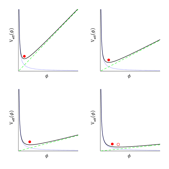
Figure 1: The effective potential, $V_{\rm eff}(\phi)$ changes as the universe expands due to the term that depends on the number density of dark matter particles. In all four pictures, the dotted line is the scalar field potential, the dashed line is the rest energy of the dark matter particles as a function of $\phi$, and the solid line is the effective potential. In the early universe (top left), the number density of the dark matter particles is large causing the line associated with it to be steep. The field rapidly settles to the minimum of the effective potential. As the universe evolves (top right), this line becomes less steep, and the minimum moves to larger $\phi$. The field (solid circle) follows the minimum until (lower left), the $3H\dot{\phi}$ term in the field equation (3) becomes comparable to the first derivative of the potential. After this time, the $3H\dot{\phi}$ term acts as an effective friction and slows the field. Eventually the field is no longer in the minimum of the potential and is moving very slowly (lower right). The open circle in the lower right plot shows the minimum of the potential, and the solid circle shows the value of the field. At this point, the field is close to constant, and the interacting dark matter starts to behave as standard cold dark matter with a fixed mass.

The evolution of the field when the field is in the minimum of the effective potential was first calculated in [33]. We reproduce and expand upon those results here. The value for the field at the minimum of the effective potential is obtained by solving for the field value that causes the first derivative of the effective potential to vanish, and the result is

$$\phi_{\rm min}=\left(\frac{\alpha K}{\lambda n_{0}}\right)^{(1/1+\alpha)}\left(\frac{a}{a_{0}}\right)^{3/(1+\alpha)}=\phi_{0}\left(\frac{a}{a_{0}}\right)^{3/(1+\alpha)}.$$ (16)

In Fig. 2 we plot the value of the scalar field as a function of $a/a_{0}$ for the case $\alpha=1$. In the early universe, the field takes the value $\phi_{\rm min}$. At $\log_{10}(a/a_{0})\sim-0.6$, the effective friction term begins to become important and slows the field down. This is seen in the plot as the actual value of the field falls below $\phi_{\rm min}$ for $\log_{10}(a/a_{0})>-0.6$.

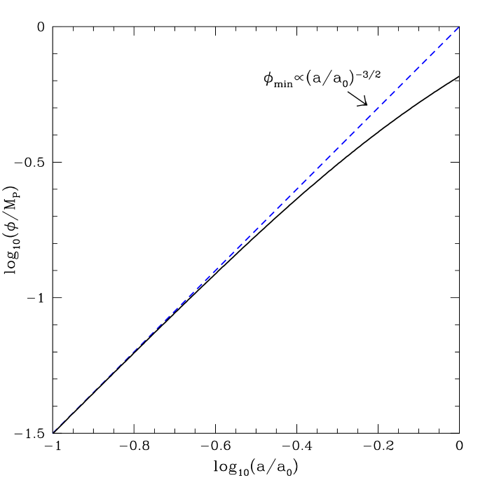
Figure 2: Plot of $\log_{10}(\phi/M_{P})$ versus $\log_{10}(a/a_{0})$ for $\alpha=1$. The dashed line shows the value of the field at the minimum of the effective potential, $\phi_{\rm min}/M_{P}$ as a function of the scale factor. The solid line represents the actual evolution of the field. In the early universe, the field sits at the minimum of the effective potential, but eventually the effective friction due to the expansion of the universe causes the field to slow down and fall behind the shifting minimum of the effective potential.

While the field remains in the minimum of the effective potential, the mass of the dark matter particles is

$$m_{DM}=\lambda\left(\frac{\alpha K}{\lambda\bar{n}_{0}}\right)^{1/(1+\alpha)}\left(\frac{a}{a_{0}}\right)^{3/(1+\alpha)},$$

and the energy density of the dark matter is

$$\rho_{DM}=\lambda\bar{n}_{0}\left(\frac{\alpha K}{\lambda n_{0}}\right)^{1/(1+\alpha)}\left(\frac{a}{a_{0}}\right)^{-3\alpha/(1+\alpha)}.$$ (17)

We next consider the energy density associated with the scalar field. When the field is at the minimum of its effective potential, and hence following (16), its time derivative is

$$\dot{\phi}=\frac{3}{1+\alpha}H\phi.$$

The magnitude of the ratio of the kinetic to potential energy of the field is then

$$\frac{\dot{\phi}^{2}}{V}\sim\frac{H^{2}\phi^{2}}{\phi^{-\alpha}}.$$ (18)

Recall, however, that in order for the field to stay in the minimum of the effective potential, the first derivative of the effective potential must be much larger than the effective friction term in the equation of motion (3) implying

$$\frac{3H\dot{\phi}}{dV/d\phi}\sim\frac{H^{2}\phi}{\phi^{-\alpha-1}}\ll 1.$$ (19)

Comparing this to (18), we see that when the field is in the minimum of the effective potential, the kinetic energy is much smaller than the potential energy of the scalar field. Thus to a good approximation, the energy density in the scalar field is

$$\rho_{\phi}=V(\phi)=K\left(\frac{\alpha K}{\lambda n_{0}}\right)^{(-\alpha/1+\alpha)}\left(\frac{a}{a_{0}}\right)^{-3\alpha/(1+\alpha)}.$$ (20)

We see from (17) and (20) that the dark matter energy density and the energy density of the scalar field have a constant ratio,

$$\frac{\rho_{DM}}{\rho_{\phi}}=\alpha,$$

while the field is in the minimum of the effective potential. Substituting (16) into (19), we find that the approximation that the field is in the minimum of the effective potential breaks down when

$$\frac{a_{*}}{a_{o}}\sim H^{-\frac{2}{3}\left(\frac{\alpha+1}{\alpha+2}\right)}\left(\frac{\lambda n_{0}}{\alpha K}\right).$$

An interesting parameter choice for this model is $\alpha=1/2$ and $(\lambda n_{0}/\alpha K)\gg 1$. In this case, there is an extended period of time during which $\rho_{DM}/\rho_{\phi}=1/2$ as is observed. We plot the relative energy densities of radiation ($\Omega_{R}$), baryons ($\Omega_{B}$), dark matter ($\Omega_{DM}$), and the scalar field ($\Omega_{\phi}$) as a function of $a/a_{0}$ in the bottom panel of Fig. 3. In the top panel, we plot the relative energy densities for a $\Lambda$CDM model for comparison.

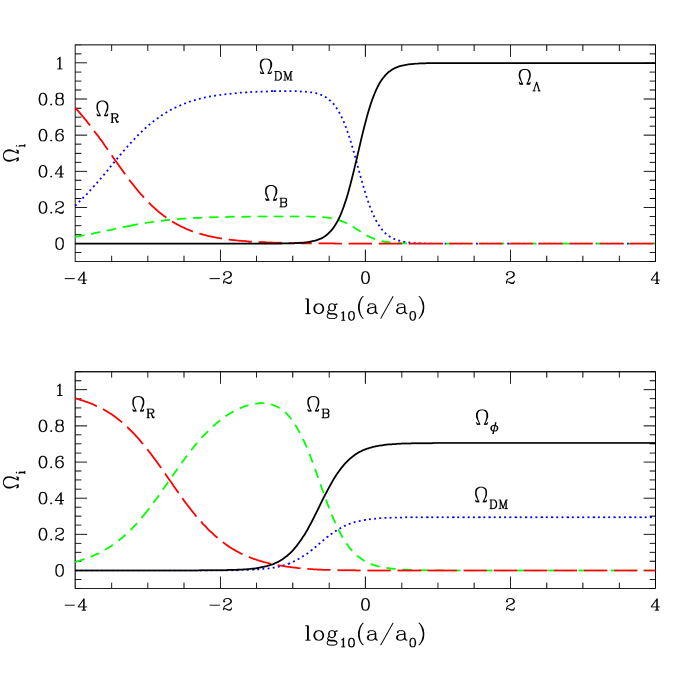
Figure 3: The bottom panel is a plot of the relative energy density in radiation ($\Omega_{R}$, long-dashed line), baryons ($\Omega_{B}$, short-dashed line), dark matter ($\Omega_{DM}$,dotted line), and the scalar field acting as the dark energy ($\Omega_{\phi}$, solid line) for $\alpha=1/2$ and $(\lambda n_{0}/\alpha K)\gg 1$. The top panel is the same plot for $\Lambda$CDM with $\Omega_{\Lambda}$, the relative energy density in the cosmological constant, replacing $\Omega_{\phi}$ and is included for comparison. Eventually, the dark energy will dominate in the interacting model, but this can be put off as long as desired by increasing $(\lambda n_{0}/\alpha K)$. Note that in this case, $\Omega_{DM}/\Omega_{\phi}=1/2$ is sustained for many e-foldings of the scale factor. Another feature of this model is that the onset of dark energy density takes place over a much longer time than in the $\Lambda$CDM scenario. Finally, the universe is never dominated by dark matter, but instead goes through an epoch of baryon domination.

For any other value of $\alpha$, we require $a_{*}/a_{0}<1$ in order to have $\rho_{DM}/\rho_{\phi}\sim 2$ today. In Fig. 4 we plot the relative energy densities in a number of models with different values of $\alpha$ and fixed $\lambda n_{0}$. Changing $\lambda n_{0}$ does not significantly alter these plots, since we must adjust the value of $K$ in order to get the right energy density in baryons and radiation today.

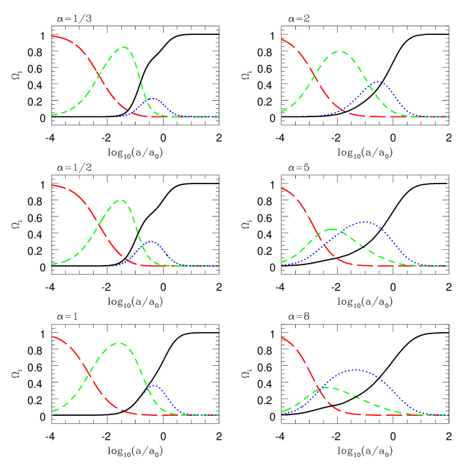
Figure 4: Plots of the relative energy density in radiation ($\Omega_{R}$, long-dashed line), baryons ($\Omega_{B}$, short-dashed line), dark matter ($\Omega_{DM}$, dotted line), and the scalar field acting as the dark energy ($\Omega_{\phi}$, solid line) vs. $log_{10}(a/a_{0})$ for various values of $\alpha$.

It is typical in models with small values of $\alpha$ that the universe is baryon dominated during structure formation, which would likely produce structure that is significantly different from what we observe. Calculating the formation of structure in these interacting dark sector models is beyond the scope of this paper. Instead, we will compare these models to observations in two other areas, the magnitude-redshift relation of SNe Ia in this section and the CMB anisotropy spectrum in the next.

Often in comparing dynamical dark energy models to SNe Ia data, one calculates the dark energy equation of state parameter, $w$, and compares this theoretical value to the values for $w$ = constant dynamical dark energy models allowed by the data. Such a comparison will not work in this case, however, because the $w$ = constant dynamical dark energy models assume that the dark matter energy density scales as $(a/a_{0})^{-3}$, which is not the case in interacting dark sector models. Thus, we must calculate the predicted magnitude-redshift relation for SNe Ia for each model and compare the predicted relation to the measured one.

The magnitude-redshift relation of SNe Ia measures the luminosity distance, $d_{L}$, as a function of redshift, $z$, via the relation

$$m-M=\log_{10}d_{L}(z),$$

where $m$ is the relative magnitude of the supernova and $M$ is its absolute magnitude. Typically, the results of these measurements are plotted as the difference between the observed $(m-M)$ and that expected from a standard model called the “empty” universe:

$$\Delta(m-M)=\log_{10}d_{L}(z)-\log_{10}d_{L}^{\,\rm empty}(z).$$

The luminosity distance is computed from the evolution of the scale factor through the relation

$$d_{L}(z)=(1+z)\int_{0}^{z}\frac{dz^{\prime}}{H(z^{\prime})},$$

and the result for the “empty” universe is

$$d_{L}^{\,\rm empty}(z)=\frac{z(1+z/2)}{H_{0}}.$$

We have calculated the theoretical $\Delta(m-M)$ for a number of models, and the results are plotted in Fig. 5 along with binned data. For comparison, we have also plotted the $\Lambda$CDM result. Note that large values of $\alpha$ do not fit the data well because they do not have enough acceleration in the expansion of the universe to match the data. Small values of $\alpha$ may also be problematic because acceleration begins too early to match the result of SN1997ff at $z\sim 1.7$. However, further high-redshift data will be required to strictly rule out such models. Similar results have also been obtained for the models considered by Amendola and his group [50].

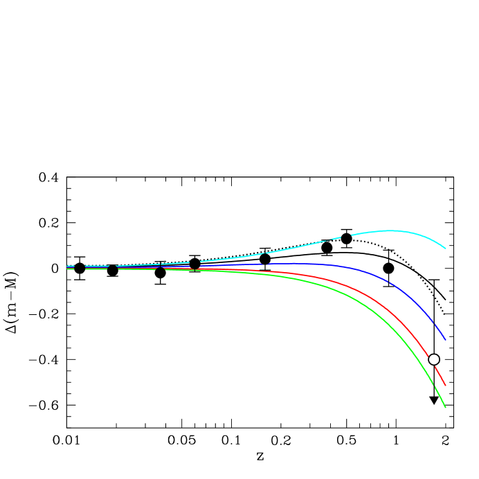
Figure 5: Comparison of several models with SNe Ia data. The solid lines lines represent models with (from top to bottom) $\alpha=1/2,1,2,5,8$. The theoretical curve for $\Lambda$CDM is shown as a dotted line for reference. The solid circles are binned SNe Ia data found in [12], and the point at $z=1.7$ is the upper limit for SN1997ff from [13]. The models with $\alpha>2$ are disfavored by moderate redshift observations.

4 Perturbations and the CMB anisotropy spectrum

In this section we derive the equations of motion for perturbations of the scalar field and the dark matter particles, which will be used in calculating the CMB anisotropy spectrum. We will work in conformal time ($ad\tau=dt$) and in the synchronous gauge where the metric is

$$ds^{2}=a^{2}(\tau)\left[-d\tau^{2}+\left(\delta_{ij}+h_{ij}\right)dx^{i}dx^{j}\right].$$

The scalar field and the dark matter energy density can be written as the sum of a background, average value and a perturbation that is assumed to be small when compared with the background value:

$$\phi=\bar{\phi}+\delta\phi$$

$$\rho_{DM}=\bar{\rho}_{DM}+\delta\rho_{DM}.$$

The dark matter perturbation has two components, the perturbation in the number density of the dark matter particles, $\delta n$, and the perturbation in the scalar field, $\delta\phi$:

$$\delta\rho_{DM}=\lambda\bar{\phi}\delta n+\lambda\bar{n}\delta\phi,$$

where $\bar{n}$ is the average number density of dark matter particles. It will be useful to also define the relative perturbation in the number density of the dark matter particles:

$$\delta_{n}=\frac{\delta n}{\bar{n}}.$$

The equations of motion for the background are (3), (7), and (8), which we reproduce here in terms of the conformal time, $\tau$:

$$\bar{\phi}^{\prime\prime}+2\frac{a^{\prime}}{a}\bar{\phi}^{\prime}+a^{2}\frac{dV}{d\bar{\phi}}=-\lambda n_{0}/a$$ (21)

$$\bar{\rho}^{\prime}_{DM}+3\frac{a^{\prime}}{a}\bar{\rho}_{DM}=\lambda\bar{n}\bar{\phi}^{\prime}$$ (22)

$$\left(\frac{a^{\prime}}{a}\right)^{2}=\frac{\rho a^{2}}{3M_{P}^{2}},$$ (23)

where a prime indicates a derivative with respect to the conformal time, $d/d\tau$. The total scalar field satisfies the equation

$$\nabla^{\mu}\nabla_{\mu}\phi+\frac{dV}{d\phi}+\lambda n=0.$$

A Fourier mode of the scalar field perturbation

$$\delta\phi_{k}(\tau)=\frac{1}{\sqrt{2\pi}}\int\delta\phi(\tau,{\bf x})e^{-i{\bf k}\cdot{\bf x}}d^{3}x$$

satisfies the equation of motion

$$\delta\phi^{\prime\prime}_{k}+2\frac{a^{\prime}}{a}\delta\phi^{\prime}_{k}+\left(k^{2}+a^{2}\frac{d^{2}V}{d\phi^{2}}\right)\delta\phi_{k}+\lambda\bar{n}a^{2}\delta_{n}=-\frac{1}{2}h^{\prime}\bar{\phi}^{\prime},$$ (24)

where we have used the background equation of motion (21) and $h$ is the trace of the metric perturbation $h_{ij}$. From here on we will suppress the subscript $k$ on the perturbed variables.

In order to get the equation of motion for the dark matter perturbation, we will need to consider the divergence of the perturbed stress-energy tensor. Let us begin by considering the perturbed stress-energy tensor for the scalar field,

$$\delta T_{(\phi)}{}^{\mu}{}_{\nu}=\left(\partial^{\mu}\delta\phi\right)\left(\partial_{\nu}\bar{\phi}\right)+\left(\partial^{\mu}\bar{\phi}\right)\left(\partial_{\nu}\delta\phi\right)-\delta^{\mu}{}_{\nu}\left(\frac{1}{2}\left(\partial_{\alpha}\delta\phi\right)\left(\partial^{\alpha}\bar{\phi}\right)+\frac{1}{2}\left(\partial_{\alpha}\bar{\phi}\right)\left(\partial^{\alpha}\delta\phi\right)+\frac{dV}{d\phi}\delta\phi\right),$$

and its divergence,

$$\nabla_{\mu}\delta T_{(\phi)}{}^{\mu}{}_{\nu} = -a^{-2}\left(\delta\phi^{\prime\prime}+2\frac{a^{\prime}}{a}\delta\phi^{\prime}+k^{2}\delta\phi+a^{2}\frac{d^{2}V}{d\phi^{2}}\delta\phi+\frac{1}{2}h^{\prime}\bar{\phi}^{\prime}\right)\partial_{\nu}\bar{\phi}$$ (25)

$$\hskip 21.68121pt-a^{-2}\left(\bar{\phi}^{\prime\prime}+2\frac{a^{\prime}}{a}\bar{\phi}^{\prime}+a^{2}\frac{dV}{d\bar{\phi}}\right)\partial_{\nu}\delta\phi$$

$$= \lambda\bar{n}\delta_{n}\left(\partial_{\nu}\phi\right)+\lambda\bar{n}\left(\partial_{\nu}\delta\phi\right),$$

where in the last line we used (21) and (24).

The perturbations to the dark matter stress-energy tensor are defined to be (following [51])

$$\delta T_{DM}{}^{0}{}_{0}=-\delta\rho_{DM}$$

$$\delta T_{DM}{}^{0}{}_{i}=-\delta T_{DM}{}^{i}{}_{0}=\bar{\rho}_{DM}v_{i}$$

The other components of the perturbed stress-energy tensor vanish. The divergence of the stress-energy of the combined dark sector must vanish to all orders. Given (25), we demand

$$\nabla_{\mu}\delta T_{DM}{}^{\mu}{}_{\nu}=-\lambda\bar{n}\delta_{n}\left(\partial_{\nu}\bar{\phi}\right)-\lambda\bar{n}\left(\partial_{\nu}\delta\phi\right).$$

The resulting equations of motion for the dark matter perturbations are

$$\delta^{\prime}_{n} = -\theta-\frac{1}{2}h^{\prime}$$ (26)

$$\theta^{\prime} = -\left(\frac{a^{\prime}}{a}+\frac{\bar{\phi}^{\prime}}{\bar{\phi}}\right)\theta+\frac{k^{2}}{a^{2}}\frac{\delta\phi}{\bar{\phi}},$$ (27)

where $\theta=ik^{j}v_{j}$.

Equations (24), (26) and (27) were integrated along with the standard equations for baryons and photons using a modified version of CMBFAST [52]. The results are plotted in Fig. 6. We were unable to fit any of the models to the WMAP CMB anisotropy spectrum [53] with values of the cosmological parameters that are consistent with other experiments. In the first five panels of Fig. 6, we show for illustrative purposes a theoretical CMB temperature anisotropy spectrum with the cosmological parameters set to the best fit values in [54] except for allowing a variation in the scalar spectral index, $n_{s}$, a parameter that describes the initial density power spectrum. Cosmic variance is shown as dotted lines, and the error bars on the binned points include only experimental error. Effective $\chi^{2}$ values were calculated for these models following [55], and were all many orders of magnitude larger than the best fit $\Lambda$CDM model. In the lower right panel, we show all five spectra evaluated with $n_{s}=1$ in order to illustrate the dependence of the spectrum on $\alpha$.

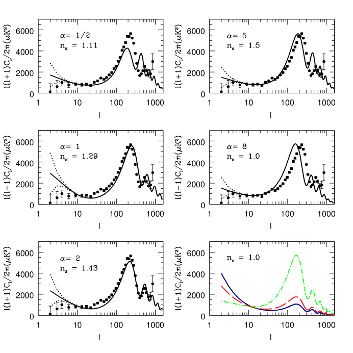
Figure 6: Plots of the CMB temperature anisotropy spectrum for several models. In the first five panels, the theoretical spectrum is compared to the WMAP results [53]. For each model, the best value of the scalar spectral index, $n_{s}$, is shown. The dotted lines represent cosmic variance. The other cosmological parameters, are set to the best fit values in [54] for illustrative purposes. In the lower right panel, we plot all five spectra with the same $n_{s}=1$, though for $\alpha=1/2,1,2$, the differences between the spectra are less than the line thickness in this plot. The solid line represents these values of $\alpha$, the long dashed line is $\alpha=5$, and the dot-dashed line is $\alpha=8$.

Much of the error in these plots is due to discrepancies between the theory and the data around the first peak in the spectrum. One can imagine, though, that a better fit around the first peak could be obtained by performing a fit over a larger number of parameters. Detailed parameter fitting, though, is beyond the scope of this paper. Even with a better fit around the first peak in the spectrum, these models face two qualitative problems in predicting the CMB temperature anisotropy spectrum, one at small scales (large $l$) due to a low value for the dark matter energy density at last scattering and the other at large scales (small $l$) due to an enhanced ISW effect (for a review of CMB physics, see [56]).

It is not surprising that these spectra look like those for a low dark matter density universe. In the models considered here, the dark matter particle mass is increasing with time. Holding the present dark matter energy density constant, a larger change in the dark matter particle mass since last scattering implies a lower value for the dark matter energy density at last scattering. At small scales, the spectra for these interacting models look very much like the spectra for $\Lambda$CDM models with a low value for $\Omega_{DM}$, models which also have a low dark matter energy density at last scattering.

The ISW effect, which affects the power in the anisotropy spectrum at large scales, is due to the integrated evolution of the gravitational potential along the path of the photons from the last scattering surface. During a matter dominated phase, large scale density perturbations evolve in a manner that keeps the gravitational potential constant. Thus, in a universe that is matter dominated from the time of last scattering to the present, no ISW effect is observed. During periods when the dominant equation of state parameter, the ratio of the pressure to the energy density of the dominant energy component of the universe $w_{d}$, is changing, the large scale gravitational potential also changes [57]. Thus, the ISW effect is observed in the $\Lambda$CDM model and in dynamical dark energy models due to the recent onset of vacuum domination and the resulting change in $w_{d}$ from zero to $-1$ [58]. In the interacting dark sector models discussed here, the onset of vacuum domination takes place over a long time, and hence $w_{d}$ is also changing over an extended time producing a large ISW effect. Moreover, the mass of the dark matter particles is increasing with time, which also causes the gravitational potential to change, and hence may cause an increase in the observed ISW effect.

The dependence of the anisotropy spectrum on $\alpha$ shown in the lower right panel of Fig. 6 is predominantly due to the dependence of the ISW effect on $\alpha$. When the scalar field is in the minimum of its effective potential, the energy density in both dark matter and dark energy scale as $(a/a_{0})^{-3\alpha/(1+\alpha)}$. This is equivalent to a model with a single fluid with an energy density evolving as $(a/a_{0})^{-3(1+w)}$ with $w=-1/(1+\alpha)$. For larger values of $\alpha$, $w$ is closer to zero, the value of $w_{\rm eff}$ during baryon domination. Hence, larger values of $\alpha$ imply a smaller change in $w_{\rm eff}$ as the universe transitions from a baryon dominated epoch to a dark matter/dark energy dominated epoch, which in turn implies a smaller ISW effect. In the spectra shown in Fig. 6, the ISW effect is larger for the smaller values of $\alpha$.

5 Conclusions

The main result of this work is a demonstration of two challenges facing cosmological models with an interaction between the dark matter and dark energy. At the outset we were concerned that an interaction that causes the mass of the dark matter particles to change in time would lead to difficulties in reproducing the measured temperature anisotropy spectrum in the CMB. In the models considered here, the mass is a monotonically increasing function of time. As a result, the energy density of the dark matter diminishes more slowly in this model than in the $\Lambda$CDM model, which in turn implies a lower ratio of dark matter energy density to radiation energy density at the time of last scattering than in $\Lambda$CDM. It was conceivable, though, that since the equations of motion for the perturbations in an interacting model differ from those in $\Lambda$CDM, some new effect could compensate for the low dark matter to radiation ratio. Having performed the calculation, we now know that this is not the case, and the initial assumption that the low dark matter to radiation ratio would be seen in the CMB temperature anisotropy spectrum was correct.

It is not difficult, however, to imagine models that can overcome this challenge. One possibility is a model in which the dark matter particle mass at the time of last scattering is comparable to the dark matter particle mass today, but varied during the intervening time. For example the dark matter particle mass could have been decreasing from a large value in the early universe, reached a minimum at some time between last scattering and today, and be increasing today. Such a model could not be ruled out by the considerations in this work, and detailed study of structure formation in such a model would be necessary to test it.

Another possibility is to finely tune the initial conditions so that the scalar field does not evolve enough from the time of last scattering to today to be ruled out by the CMB data. In the models considered here, generic initial conditions lead to the scalar field sitting in the minimum of its effective potential for a significant time. One could finely tune the initial conditions so that the scalar field does not reach its minimum, and the effective friction due to the expansion of the universe prevents the field from evolving too much so that it can satisfy the CMB constraints. Such a situation, though aesthetically displeasing, still remains a possibility. A similar effect can also be obtained by either introducing a new dark sector field or a different potential that holds the field near a fixed value. Ruling out these situations would again require a more detailed study of structure formation, and this is the approach of [35].

The second challenge to interacting models is avoiding an enhanced ISW effect at small $l$ in the CMB temperature anisotropy spectrum. One of the potential aesthetic benefits of an interacting dark sector model is that the transition from a dark matter dominated epoch to a vacuum dominated epoch takes place over an extended period of time when compared to $\Lambda$CDM, thus softening the coincidence problem. Unfortunately, this work has demonstrated that, at least in the specific model considered here, allowing the dominant effective equation of state parameter to vary from zero during matter domination to nearly $-1$ during vacuum domination over too long a time leads to an enhanced ISW effect that is in conflict with observation. The methods discussed above to overcome the challenge of a time varying dark matter particle mass would likely also overcome this challenge as well. Such models allow for only small deviations from $\Lambda$CDM and more standard dynamical dark energy models, and hence the evolution of the effective equation of state parameter would be similar to $\Lambda$CDM and not differ from what is observed.

In this work we have used the CMB temperature anisotropy spectrum to rule out a class of cosmological models with an interaction between the dark matter and dark energy. These models, however, are only among the simplest possibilities for such an interaction. More complicated models may well overcome the challenges pointed out here, and with strict new observational tests of the $\Lambda$CDM model on the way, it will be useful to continue to study interacting dark sector models.

References

- [1] M. Persic, P. Salucci and F. Stel, Mon. Not. Roy. Astron. Soc. 281, 27 (1996) [arXiv:astro-ph/9506004].
- [2] N. A. Bahcall, arXiv:astro-ph/9612046.
- [3] J. R. Primack, arXiv:astro-ph/9707285.
- [4] W. L. Freedman, Phys. Scripta T85, 37 (2000) [arXiv:astro-ph/9905222].
- [5] M. S. Turner, Phys. Scripta T85, 210 (2000) [arXiv:astro-ph/9901109].
- [6] M. S. Turner, “The case for Lambda-CDM”, in Critical Dialogues in Cosmology, N. Turok ed., World Scientific (1997) [arXiv:astro-ph/9703161].
- [7] C. L. Bennett et al., arXiv:astro-ph/0302207.
- [8] C. B. Netterfield et al. [Boomerang Collaboration], Astrophys. J. 571 (2002) 604 [arXiv:astro-ph/0104460].
- [9] N. W. Halverson et al., Astrophys. J. 568, 38 (2002) [arXiv:astro-ph/0104489].
- [10] A. G. Riess et al. [Supernova Search Team Collaboration], Astron. J. 116, 1009 (1998) [arXiv:astro-ph/9805201].
- [11] S. Perlmutter et al. [Supernova Cosmology Project Collaboration], Astrophys. J. 517, 565 (1999) [arXiv:astro-ph/9812133].
- [12] J. L. Tonry et al., arXiv:astro-ph/0305008.
- [13] A. G. Riess et al., Astrophys. J. 560, 49 (2001) [arXiv:astro-ph/0104455].
- [14] S. M. Carroll, Living Rev. Rel. 4, 1 (2001) [arXiv:astro-ph/0004075].
- [15] P. J. Peebles and B. Ratra, Rev. Mod. Phys. 75, 599 (2003) [arXiv:astro-ph/0207347].
- [16] T. Padmanabhan, Phys. Rept. 380, 235 (2003) [arXiv:hep-th/0212290].
- [17] C. Wetterich, Nucl. Phys. B 302, 668 (1988).
- [18] B. Ratra and P. J. Peebles, Phys. Rev. D 37, 3406 (1988).
- [19] J. A. Frieman, C. T. Hill, A. Stebbins and I. Waga, Phys. Rev. Lett. 75, 2077 (1995) [arXiv:astro-ph/9505060].
- [20] R. R. Caldwell, R. Dave and P. J. Steinhardt, Phys. Rev. Lett. 80, 1582 (1998) [arXiv:astro-ph/9708069].
- [21] C. Armendariz-Picon, T. Damour and V. Mukhanov, Phys. Lett. B 458, 209 (1999) [arXiv:hep- th/9904075].
- [22] C. Armendariz-Picon, V. Mukhanov and P. J. Steinhardt, Phys. Rev. Lett. 85, 4438 (2000) [arXiv:astro-ph/0004134].
- [23] C. Armendariz-Picon, V. Mukhanov and P. J. Steinhardt, Phys. Rev. D 63, 103510 (2001) [arXiv:astro-ph/0006373].
- [24] L. Mersini, M. Bastero-Gil and P. Kanti, Phys. Rev. D 64, 043508 (2001) [arXiv:hep-ph/0101210].
- [25] R. R. Caldwell, Phys. Lett. B 545, 23 (2002) [arXiv:astro-ph/9908168].
- [26] S. M. Carroll, M. Hoffman and M. Trodden, arXiv:astro-ph/0301273.
- [27] V. Sahni and A. A. Starobinsky, Int. J. Mod. Phys. D 9, 373 (2000) [arXiv:astro-ph/9904398].
- [28] L. Parker and A. Raval, Phys. Rev. D 60, 063512 (1999) [arXiv:gr-qc/9905031].
- [29] A. Melchiorri, L. Mersini, C. J. Odman and M. Trodden, arXiv:astro-ph/0211522.
- [30] I. Maor, R. Brustein, J. McMahon and P. J. Steinhardt, Phys. Rev. D 65, 123003 (2002) [arXiv:astro-ph/0112526].
- [31] J. A. Casas, J. Garcia-Bellido and M. Quiros, Class. Quant. Grav. 9, 1371 (1992) [arXiv:hep-ph/9204213]. J. Garcia-Bellido, Int. J. Mod. Phys. D 2, 85 (1993) [arXiv:hep-ph/9205216].
- [32] C. Wetterich, Astron. Astrophys. 301, 321 (1995) [arXiv:hep-th/9408025].
- [33] G. W. Anderson and S. M. Carroll, arXiv:astro-ph/9711288.
- [34] R. Bean, Phys. Rev. D 64, 123516 (2001) [arXiv:astro-ph/0104464].
- [35] G. R. Farrar and P. J. Peebles, arXiv:astro-ph/0307316.
- [36] L. Amendola, Phys. Rev. D 62, 043511 (2000) [arXiv:astro-ph/9908023].
- [37] L. Amendola and D. Tocchini-Valentini, Phys. Rev. D 64, 043509 (2001) [arXiv:astro-ph/0011243].
- [38] L. Amendola and D. Tocchini-Valentini, Phys. Rev. D 66, 043528 (2002) [arXiv:astro-ph/0111535].
- [39] L. Amendola, C. Quercellini, D. Tocchini-Valentini and A. Pasqui, Astrophys. J. 583, L53 (2003) [arXiv:astro-ph/0205097].
- [40] D. Comelli, M. Pietroni and A. Riotto, arXiv:hep-ph/0302080.
- [41] L. Amendola and C. Quercellini, arXiv:astro-ph/0303228.
- [42] M. Gasperini, F. Piazza and G. Veneziano, Phys. Rev. D 65, 023508 (2002) [arXiv:gr-qc/0108016].
- [43] A. de la Macorra, arXiv:astro-ph/0212275.
- [44] G. Mangano, G. Miele and V. Pettorino, Mod. Phys. Lett. A 18, 831 (2003) [arXiv:astro-ph/0212518].
- [45] M. Doran and J. Jaeckel, Phys. Rev. D 66, 043519 (2002) [arXiv:astro-ph/0203018].
- [46] R. R. Khuri, arXiv:astro-ph/0303422.
- [47] W. Zimdahl and D. Pavon, Phys. Lett. B 521, 133 (2001) [arXiv:astro-ph/0105479].
- [48] W. Zimdahl and D. Pavon, Gen. Rel. Grav. 35, 413 (2003) [arXiv:astro-ph/0210484].
- [49] L. P. Chimento, A. S. Jakubi, D. Pavon and W. Zimdahl, Phys. Rev. D 67, 083513 (2003) [arXiv:astro-ph/0303145].
- [50] L. Amendola, Mon. Not. Roy. Astron. Soc. 342, 221 (2003) [arXiv:astro-ph/0209494].
- [51] C. P. Ma and E. Bertschinger, Astrophys. J. 455, 7 (1995) [arXiv:astro-ph/9506072].
- [52] U. Seljak and M. Zaldarriaga, Astrophys. J. 469, 437 (1996) [arXiv:astro-ph/9603033].
- [53] G. Hinshaw et al., arXiv:astro-ph/0302217.
- [54] D. N. Spergel et al., arXiv:astro-ph/0302209.
- [55] L. Verde et al., arXiv:astro-ph/0302218.
- [56] W. Hu and S. Dodelson, Ann. Rev. Astron. Astrophys. 40, 171 (2002) [arXiv:astro-ph/0110414].
- [57] J. M. Bardeen, Phys. Rev. D 22, 1882 (1980).
- [58] K. Coble, S. Dodelson and J. A. Frieman, Phys. Rev. D 55, 1851 (1997) [arXiv:astro-ph/9608122].