Star formation and the environment of nearby field galaxies

Abstract

We investigate the environmental dependence of galaxies with star formation from a volume-limited sample of $4782$ nearby field galaxy spectra extracted from the 2dF Galaxy Redshift Survey final data release. The environment is characterized by the local spatial density of galaxies, estimated from the distance to the 5th nearest neighbour. Extensive simulations have been made to estimate correction factors for the local density due to sample incompleteness. We discriminate the galaxies in distinct spectral classes – passive, star-forming, and short starburst galaxies – by the use of the equivalent widths of [O ii]$\lambda$3727 and H$\delta$. The frequency of galaxies of different classes are then evaluated as a function of the environment. We show that the fraction of star-forming galaxies decreases with increasing density, whereas passive galaxies present the opposite behaviour. The fraction of short starburst galaxies – that suffered a starburst at $\sim$ 200 Myr ago – do not present strong environmental dependence. The fraction of this class of galaxies is also approximately constant with galaxy luminosity, except for the faintest bins in the sample, where their fraction seems to increase. We find that the star-formation properties are affected in all range of densities present in our sample (that excludes clusters), what supports the idea that star-formation in galaxies is affected by the environment everywhere. We suggest that mechanisms like tidal interactions, which act in all environments, do play a relevant role on the star-formation in galaxies.

1 INTRODUCTION

It has become clear along the last decades that the environment a galaxy inhabits has a profound impact on its star-formation properties. Indeed, the study of the variations of star formation in galaxies as a function of their environment has a great importance for extragalactic astronomy, since it makes possible to understand some properties of the formation and evolution of galaxies in the Universe, helping to discriminate between ‘nature’ and ‘nurture’ effects.

It is well known that at low redshifts star-forming galaxies constitute a small population in high-density regions, especially in galaxy clusters. Osterbrock (1960) observed that the frequency of emission-line galaxies is lower in clusters than in the field. Later, this trend was verified in a quantitative way by many works (Gisler, 1978; Dressler, Thompson & Shectman, 1985; Abraham et al., 1996; Balogh et al., 1999; Poggianti et al., 1999; Loveday, Tresse & Maddox, 1999; Ellingson et al., 2001, and others). Furthermore, it is also known the trend for H i deficiency among cluster spirals galaxies (Giovanelli & Haynes, 1985; Solanes et al., 1996; Bravo-Alfaro et al., 2000; Goto et al., 2003), that could explain the interruption of star formation in terms of the depletion of the galaxy gaseous content, either by its consumption or suppression (Gisler, 1978; Kennicutt, 1983; Kenney & Young, 1989). On the other side, some works show that spirals in clusters may have a star formation rate similar or even larger than field spirals (Gavazzi & Jaffe, 1985; Moss & Whittle, 1993; Gavazzi et al., 1998; Biviano et al., 1997), although, as suggested by Gavazzi & Jaffe, the observed increment in the star-formation rate of these galaxies may be a transient phenomenon, which occurs while the galaxy suffers the suppression of its gaseous content. In low-density environments, tidal interactions are the most relevant process. Ordinary star-forming galaxies have an external gaseous reservoir that is critically important to the continuous gas supply of the galaxy disk. Numerical simulations (Bekki, Couch & Shioya, 2001) show that this reservoir is fragile and, consequently, more susceptible to tidal effects.

Effects of the environment on the star-formation in galaxies, then, must involve at least two types of processes: i) those that decrease the gaseous content and, therefore, reduce the potential of star formation in galaxies, and ii) processes that trigger bursts of star formation. Among the first class of process there are: interactions between the intragalactic and intergalactic medium, including gas removal and evaporation (Gunn & Gott, 1972; Fujita & Nagashima, 1999); tidal interactions, that remove the gas of the disk of spiral galaxies (Byrd & Valtonen, 1990); suppression of the accretion of gas-rich materials in the neighbourhood of the galaxy (Larson, Tinsley & Caldwell, 1980; Bekki, Couch & Shioya, 2001). The second type of processes include: gas compression by ram-pressure, that induces star formation (Dressler & Gunn, 1983; Bothun & Dressler, 1986; Vollmer et al., 2001); fusion with other systems (Barnes & Hernquist, 1991; Lavery & Henry, 1994; Bekki, 2001); tidal interactions (Moss & Whittle, 2000). Thus, process like tidal interactions may trigger star-formation as well as may contribute to its end.

Recent galaxy surveys are allowing to investigate the relation between star formation and environment with large samples of data collected in a uniform way. This includes the Las Campanas Redshift Survey (Hashimoto et al., 1998), the 15R-North Galaxy Redshift Survey (Carter et al., 2001), the 2dF Galaxy Redshift Survey (2dFGRS, Lewis et al., 2002), and the Sloan Digital Sky Survey (SDSS, Gómez et al., 2003). Lewis et al. (2002) have analyzed the environmental dependence of star formation rates (SFRs) near galaxy clusters in the 2dFGRS region, finding that there is a correlation between SFR and projected density, that disappears below $\sim 1$ h₇₀ galaxy Mpc^-2 (for galaxies brighter than $M_{b}=-19$). The SDSS data shows a strong correlation between SFR and local projected density, with a “break” in this relation at the same density found near the 2dFGRS clusters; below this threshold, corresponding to a clustercentric radius of $\sim$ 3 virial radii, the SFR varies slowly with local projected density.

In this work, instead of focusing on the SFR, we analyse the environmental dependence of the population of star-forming nearby field galaxies ($z<0.05$) based on a volume-limited sample extracted from the 2dFGRS final data release (Colless et al., 2003). The star formation is characterized by spectral classes defined using the equivalent widths of [O ii]$\lambda$3727 and H$\delta$. The environmental parameter is the local spatial density of galaxies. The paper is organized as follows. Section 2 presents the sample selection, the method adopted for the density estimation, and the spectral indices that will be analysed here. Section 3 describes the spectral classification and presents the relation between the fraction of distinct galaxy types and environment in our sample. Our results are discussed in Section 4. Finally, in Section 5 we summarize our conclusions.

2 The sample and the estimation of local galaxy density

In this section we describe the sample of galaxies that will be analysed and present the parameter that will be used to describe a galaxy environment, the local galaxy density. We also present the spectral indices that will be used to describe star-formation properties of the galaxies. Finally, we discuss the selection function of the sample.

2.1 Limited volume sample

The data used in this work were extracted from the 2dFGRS spectra recently available on the final data release (Colless et al., 2003, see also Colless et al. 2001 for further and detailed information about the survey). The 2dFGRS obtained spectra for 245591 objects, mainly galaxies, brighter than an extinction-corrected magnitude limit of $b_{J}=19.45$. We have constructed a limited volume sample with galaxies within the strips located in the Northern (NGP; $2.5^{\circ}>\delta>-7.5^{\circ}$, $9^{h}50^{m}<\alpha<14^{h}50^{m}$) and in the Southern Galactic hemispheres (SGP; $-22.5^{\circ}>\delta>-37.5^{\circ}$, $21^{h}40^{m}<\alpha<3^{h}40^{m}$). The sample comprises galaxies with radial velocities between 600 and 15000 km s^-1 brighter than an extinction corrected absolute magnitude $M_{b_{J}}^{lim}=-17.38+5\log h$, corresponding to corrected apparent magnitudes $b_{J_{lim}}\leq 18.50$. The advantage of this approach is that the radial selection function is uniform (in the case of complete sampling) and variations in the space density of galaxies within the volume are due to clustering only (Norberg et al., 2002). Considering only galaxies with spectra with quality parameter $Q\geq 3$ (Colless et al., 2001), this initial sample contains 8040 galaxies. As will be shown in Section 3.2, the fraction of star-forming galaxies increases with the limiting absolute magnitude of the sample, and hence our results regarding the fraction of spectral classes are also dependent on this parameter.

Since we are interested in field galaxies, it is necessary to remove from the sample galaxies that are members of galaxy clusters. The clusters within the 2dFGRS region were studied by De Propris et al. (2002), and their cluster catalogue may be considered complete up to $z=0.1$, well above the limit of our volume limited sample. The studies of Gómez et al. (2003) and Lewis et al. (2002) for the SDSS and 2dFGRS, respectively, indicate that a representative sample of field galaxies cannot be obtained within $\sim$ 3 to 4 virial radius of the cluster core. The virial radius of a cluster can be calculated as $R_{V}=0.002~{}\sigma_{r}~{}h^{-1}$ Mpc, where $\sigma_{r}$ is the radial velocity dispersion in units of km s^-1 (Girardi et al., 1998), and for the clusters studied by Gómez et al. (2003) its mean value is $\sim~{}1~{}h^{-1}$ Mpc. Consequently, we excluded from the sample (as well as from the simulations described below) all galaxies inside a sphere of 4 $h^{-1}$ Mpc radius around the cluster centers catalogued by De Propris et al. (2002). The resulting sample of field galaxies contains $6768$ galaxies.

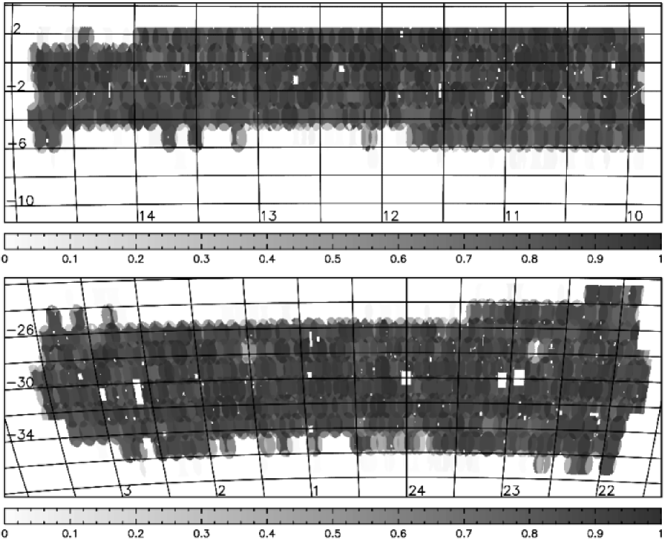
Figure 1: Redshift completeness as a function of position for the simulated galaxies. The top panel is for the NGP strip and the bottom panel is for the SGP strip. The horizontal axis represents the right ascension (in hours) and the vertical axis is the declination (in degrees). The completeness, between 0 and 1, is represented by different levels of intensity, with darker regions representing regions of higher completeness, following the scale shown below the strips.

2.2 Simulations

Despite the fact that the 2dFGRS final data release has a high completeness, this is not true for some regions covered by the survey, and we need to take into account the possibility of survey incompleteness in the determination of the environment associated to each object in our sample. With this aim, we generated mock catalogues to simulate the distribution of galaxies in our selected volume and the distribution of the objects selected by the 2dFGRS. Firstly, we computed the mean galaxy number density brighter than the adopted luminosity limit:

$$\bar{\rho}(>L_{min})=\int^{\infty}_{L_{min}}\Phi(L)dL$$ (1)

where $\Phi(L)$ is the Schechter luminosity function with parameters (in $b_{J}$ band) $M^{*}=-19.66+5\log h$, $\alpha=-1.21$ and $\Phi^{*}=1.66\times 10^{-2}\,h^{3}$Mpc^-3 (Norberg et al., 2001), that are appropriate for the 2dFGRS. Then, for the NGP and SGP regions, we evaluated the mean galaxy number in each region, $\bar{N}$, that would be expected for a uniform galaxy distribution in each volume. After, for each simulation, we assumed a Gaussian distribution (with mean $\bar{N}$ and dispersion ${\bar{N}}^{1/2}$) to determine the actual number of galaxies, $N$, included in each volume. Finally, for the $N$ galaxies in each region we have randomly selected a position ($\alpha$, $\delta$), a luminosity (based on the Schechter luminosity function) and a redshift, assuming a uniform distribution within each volume.

At this point we need to verify how the incompleteness of the survey affects the simulated catalogues. Colless et al. (2001) present a description of the magnitude and completeness masks that were constructed for this purpose. The redshift completeness is given by a parameter called $R$, which depends on the position at the strips covered by the survey and is the ratio between the observed number of objects and the total number of objects in the parent catalogue at that position. Moreover, the masks supply a magnitude limit and a $\mu$ parameter that also depends on the position. The redshift completeness is magnitude dependent and, as shown by Norberg et al. (2001), it can be written as

$$c_{z}(b_{J},\mu_{i})=0.99\;[1-\exp\,(b_{J}-\mu_{i})].$$ (2)

Thus, in a second stage of the simulations, we have applied the completeness masks to our simulated data to select a sample of simulated galaxies with spectra within each region. In this way, each simulation results, for each region, in two volume-limited samples, one that represents the ‘parent’ galaxy distribution in the range of redshifts and magnitudes considered here, and another simulating the sub-sample of galaxies with 2dFGRS spectra. This approach allows to define a correction factor to the measured local galaxy density, that will be discussed in the next section. In Fig. 1 we show the completeness map resulting from the simulations for the two strips covered by the survey (for comparison, see maps shown in Colless et al. 2003).

2.3 Local spatial density of galaxies

In recent studies, the environment has been characterized either by the local number galaxy density (e.g., Hashimoto et al., 1998; Carter et al., 2001), or by the projected galaxy density (e.g., Lewis et al., 2002; Gómez et al., 2003).

We adopted a non-parametric method to determine the local number density of galaxies, based on the $k$th nearest neighbour density estimator ($k$NN). This method fix a value for $k$ and let the volume $V$, centred on a given object and extending to its $k$th nearest neighbour, be a random variable. This volume is large in low density regions and small in high density regions. The $k$NN density estimator may be written as (Casertano & Hut, 1985; Fukunaga, 1990):

$$\rho=\frac{k-1}{V(r)}$$ (3)

with $V(r)=4\pi r^{3}/3$, where $r$ is the distance to $k$th nearest neighbour. For our purposes we have used the value $k=5$. We have made tests for several values of $k$, concluding that 5 is an adequate choice, given the shape of the survey regions, that does not favour larger values. Additionally, we have prevented an incorrect density estimate due to border effects by excluding galaxies whose $k$th neighbours have projected distances greater than the distance of the galaxy to the closest border of the survey region or of the sample volume.

To correct the estimated density for sample incompleteness, we have generated $800$ pairs of simulated catalogues, each pair comprising a ‘parent’ and an ‘observed’ sample. This procedure allowed us to compute a mean local correction factor for the density, $\mathcal{C}$, given by

$$\mathcal{C}=<\frac{\rho_{p}}{\rho_{o}}>,$$ (4)

where $\rho_{p}$ is the number density associated with the ‘parent’ sample and $\rho_{o}$ is the same for the ‘observed’ sample.

Figure 2: Distribution of the local galaxy density correction factor ($\mathcal{C}$). The filled circle represents the median value and the error bars are the respective quartiles of the distribution of $\mathcal{C}$ values. The arrow indicates the upper limit in $\mathcal{C}$ adopted to select the sample.

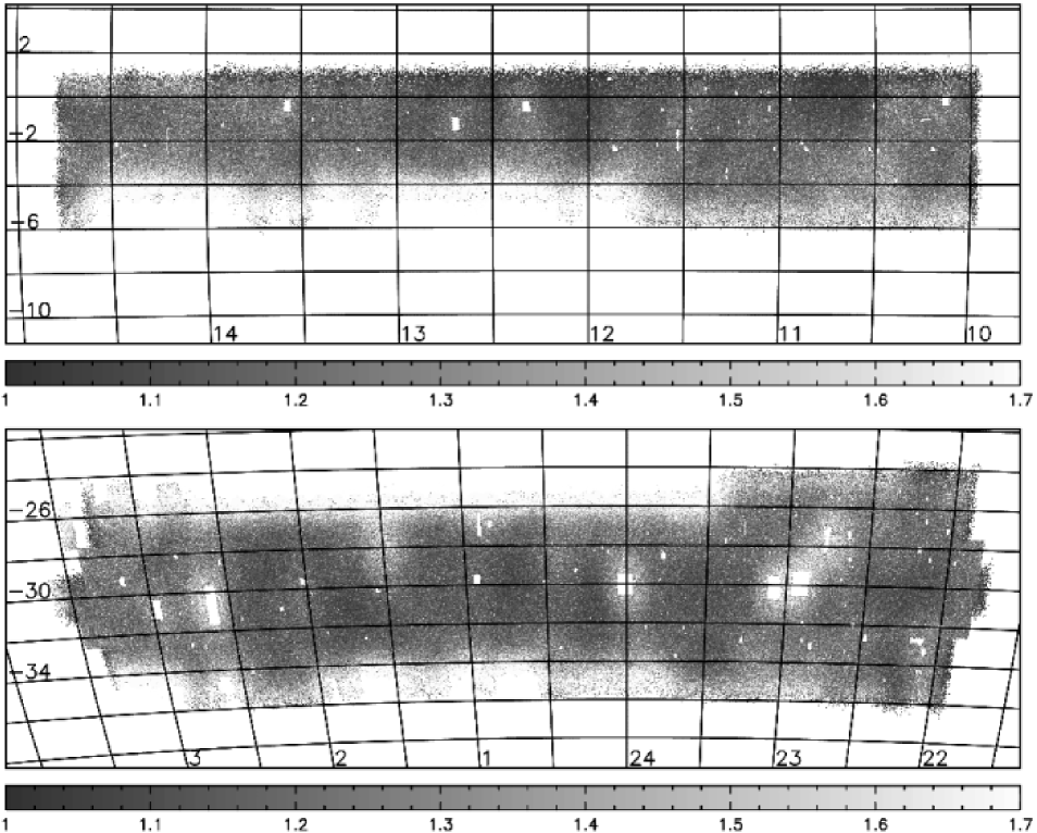
Figure 3: Correction factor, $\mathcal{C}$, as a function of position for the selected regions. The top panel is for the NGP strip and the bottom panel is for the SGP strip. The horizontal axis represents the right ascension (in hours) and the vertical axis is the declination (in degrees).The values of $\mathcal{C}$ are represented by different levels of intensity, with darker regions representing regions of lower corrections, accordingly to the scale shown below the strips.

The local values of $\mathcal{C}$ were then used to correct the density associated to each galaxy in our initial volume-limited sample. Fig. 2 shows the distribution of $\mathcal{C}$ for this sample. The filled circle represents the median value of the distribution and the error bars are the respective quartiles. Note that, by definition, $\mathcal{C}\geq 1$. To avoid uncertainties introduced in the density by large corrections, we have restricted the sample to those objects located in regions where $1\leq\mathcal{C}\leq 1.7$; in Fig. 2 this limit is indicated by an arrow.

Since we are neglecting peculiar velocities in distance estimates, galaxies in dense environments, where the velocity dispersion is high, will probably have their local densities underestimated. However, since we have removed from the sample galaxies within $\sim 4$ virial radius around the clusters in the 2dFGRS survey area (c.f. Sect. 2.1), our results should not be strongly affected by peculiar velocities.

At this point, the sample volume is $\sim 14400\,h^{-3}\,$Mpc³ and contains $5463$ galaxies. In Fig. 3 we present the correction factor as a function of position for the two strips covered by the survey, where we only show the regions comprising the selected sample that follows the constraints on $\mathcal{C}$.

2.4 Measurements of spectral indices

For each galaxy in our sample we measured the total (i.e, emission plus absorption) equivalent widths (EWs) of [O ii]$\lambda$3727, H$\delta$, H$\beta$, [O iii]$\lambda$5007, [N ii]$\lambda$6548, H$\alpha$ and [N ii]$\lambda$6583 directly from the 2dFGRS spectra; hereafter these quantities will be called ‘spectral indices’. We adopt here positive values for emission line EWs, and negative for absorption EWs. The indices were computed by fitting the continuum defined in two regions around the line (blue and red continuum) and measuring the line flux normalized relative to this continuum. The EW errors were computed following the prescription of Cid Fernandes et al. (2001), that takes into account the noise within the line window and the uncertainty in the positioning of the continuum.

In Section 3 we will make a spectral classification based on the [O ii]$\lambda$3727 and H$\delta$ EWs. This pair of indices is convenient because it can be measured even at high redshifts and, thus, it can be used directly to probe evolutionary effects in samples of more distant galaxies. The median values of these indices are very similar to those obtained by Balogh et al. (1999) for a sample of field galaxies extracted from the CNOC1 sample; our EW[O ii] has also mean and median values comparable to those obtained by Gómez et al. (2003) for a SDSS sub-sample. The median errors (with the quartiles of the error distribution) are $3.3^{+1.7}_{-0.9}$ and $1.8^{+1.0}_{-0.6}$ Å for [O ii]$\lambda$3727 and H$\delta$, respectively. The error distribution has a long tail towards large errors and, thus, we excluded from the analysis $456$ objects with EW uncertainties larger than $10$ Å for EW([O ii]) and $6$ Å for EW(H$\delta$). Additionally, following Lewis et al. (2002), we excluded $225$ galaxies with EW(H$\alpha$) $>10$ Å and EW([N ii]$\lambda$6583) $>0.55\,$EW(H$\alpha$). These objects are classified as active galactic nuclei (AGNs) and have been removed from the sample because they have a significant non-thermal component (Veilleux & Osterbrock, 1987), contrarily to typical star-forming H ii regions.

A point that deserves mention here is the bias that may be introduced in the analysis due to the use of small fibers to measure the galaxy spectra. This effect, known as aperture bias, is discussed in detail by Kochanek, Pahre & Falco (2000), who demonstrated that it can lead to an underestimate of EW values, and consequently, to an overestimate of the fraction of early-type galaxies in a survey. Madgwick et al. (2002) discuss the presence of this effect in 2dFGRS spectra, concluding that it does not introduce any significant bias in the fractions of galaxies distinguished accordingly to their spectral types. We will return to this point in Section 4.

2.5 The selected sample

After the exclusion of the objects with high uncertainties in the spectral indices and those identified as AGNs, the final sample comprises $4782$ galaxies, whose properties will be analysed and discussed in the following sections.

The sample completeness may be described by a selection function $S(b_{J})$ that we present in Fig. 5. This function is defined as

$$S(b_{J})=\frac{N_{sel}}{N_{T}},$$ (5)

where, for a given magnitude bin, $N_{sel}$ is the number of selected galaxies and $N_{T}$ is the total number in the volume. Fig. 4 shows that the selection function remains constant, and with maximum value, until $b_{J}\sim 14.0$. For $14.0\la b_{J}\la 14.5$ the function presents a variable behaviour and, for fainter magnitudes, it is approximately constant, decreasing for $b_{J}\ga 17.0$ and reaching the final value $S(b_{J})\sim 0.88$. Fig. 5 shows the distribution of magnitudes for the selected objects (dashed line) and for the initial sample (solid line). This figure suggests that our selection procedures did not introduce any significant bias in the magnitude distribution of our final sample.

Figure 4: Selection function as a function of apparent magnitude (b_J) for the selected sample.

Figure 5: Magnitude distribution for the initial sample (with N${}_{T}=5463$ galaxies), shown as a solid line, and for the selected galaxies (N${}_{Sel}=4782$), shown as a dashed line.

3 SPECTRAL CLASSIFICATION AND ANALYSIS

3.1 Spectral classification

Several authors have used EWs in galaxy classification (e.g., Hamilton, 1985; Poggianti et al., 1999; Balogh et al., 1999; Bekki, Shioya & Couch, 2001; Poggianti, Bressan & Fransceschini, 2001). One advantage of EWs is that they are not affected by extinction, although they are sensitive to differences in the extinction of the regions that produce the emission lines and those producing the continuum (the selective extinction; e.g., Stasińska & Sodré, 2001). Moreover, EWs are relatively insensitive to changes in instrumental resolution and they can be measured in non-flux calibrated spectra, like the 2dFGRS data.

Here we adopt the [O ii] and H$\delta$ EWs to classify the galaxies in the sample. These lines can be measured up to large redshifts, and thus our results may be considered a $z=0$ calibration for evolutionary studies of the environmental dependence of the fraction of star forming galaxies. The EW of the [O ii]$\lambda$3727 doublet is associated with the presence of young, massive stars, and is a useful tracer of star formation at the blue side of an optical spectrum. For this reason it has been adopted in many studies of star formation properties in galaxies. In fact, works as those of Gallagher, Hunter & Bushouse (1989), Kennicutt (1992), and Tresse et al. (1999) have shown that the [O ii] line presents a good correlation with primary tracers of star formation, like H$\beta$ and H$\alpha$ emission lines. The other spectral index we adopted for the spectral classification is the EW of the Balmer line H$\delta$. When in emission, this feature is produced in objects with high increment in the star formation rate. On the other hand, strong absorption in H$\delta$ is associated to galaxies which had an intense starburst ended about 1–2 Gyr ago (Barbaro & Poggianti, 1997). Following Balogh et al. (1999), in this work we will classify galaxies in spectral classes accordingly to their position in the EW([O ii])–EW(H$\delta$) plane, which relates an index linked to star formation activity to another associated with starburst age. Additionally, we define an object as a star-forming galaxy if it has EW([O ii]) $>5\;$Å, that is about $1.5\sigma$ above our detection limit. It is also important to note again that we use positive values to indicate emission lines and negative values for absorption lines. We adopt here 3 spectral classes (see Balogh et al., 1999):

• passive galaxies (P: EW([O ii]) $\leq$ 5 Å): galaxies without evidence of significant current star formation (in general E or S0);

• short starburst galaxies (SSB: EW([O ii]) $>$ 5 Å, EW(H$\delta$) $>$ 0): galaxies where a large fraction of the light comes from a starburst that started less than $\sim$ 200 Myr ago;

• ordinary star-forming galaxies (SF: EW([O ii]) $>$ 5 Å, EW(H$\delta$) $<$ 0): includes most normal spirals and irregulars, that have been forming stars for several hundred million years.

Figure 6: The EW([O ii])–EW(H$\delta$) plane, indicating the regions that define the three spectral classes (P, SF, SSB) discussed in this work.

Fig. 6 shows the EW([O ii])–EW(H$\delta$) plane with the distribution of galaxies in the regions of each spectral class. The total number of galaxies with star formation is $N_{TSF}=2750$, of which $N_{SSB}=285$ and $N_{SF}=2465$, and the number of those without evidence of ongoing star formation is $N_{P}=2032$. Considering only galaxies with star formation, SSBs correspond to $\sim 10$% of the total. This fraction compares very well with that obtained by Balogh et al. for a sample of field galaxies ($\sim 9$% of star-forming galaxies). Note that the classification of Balogh et al. also includes other two classes: K+A e A+em. These classes comprise galaxies with strong H$\delta$ absorption (EW(H$\delta$) $<$ $-5$ Å). In our classification, the K+A galaxies belongs to the P class and the A+em are in the SF class.

It is worth mentioning that the 2dFGRS database provides for each galaxy a spectral type, derived from a Principal Component Analysis of the spectra (Madgwick et al., 2002). These spectral types are strongly correlated with EW(H$\alpha$) and, consequently, they follow the same trends than EW(H$\alpha$).

3.2 Correlations with luminosity

The fraction of galaxies in each spectral class (relative to the total number of objects in the selected sample), is shown in Fig. 7 as a function of the absolute magnitude. The fractions of SF and P classes show a strong correlation with luminosity: low-luminosity objects are essentially galaxies that present evidence of star formation activity, generally late-type spirals and irregulars; the opposite is seen for brighter objects, which include mainly passive galaxies. The population of SSB galaxies present an excess of objects with low luminosity, with their fraction increasing for $M_{b_{J}}-5\log h\ga-18$; SSB galaxies brighter than this value do not show trends with luminosity.

Figure 7: Fraction of galaxies in each spectral class as a function of the absolute magnitude. For each class, each magnitude bin contains about the same number of objects; the error bars were computed assuming a Poissonian statistics.

Relations between star formation and luminosity as those shown in Fig. 7 have been detected in many surveys. Indeed, the luminosity function of nearby galaxies, divided accordingly to the presence or lack of the [O ii] emission line, has been calculated for the Las Campanas Redshift Survey (Lin et al., 1996) and the ESO Slice Project (Zucca et al., 1997), as well as for the 2dFGRS (Folkes et al., 1999; Madgwick et al., 2002). These studies have found that star-forming galaxies tend to be less luminous than passive galaxies. These results are also confirmed by studies of luminosity function of samples selected by morphological (Marzke et al., 1998) and spectral types (Bromley et al., 1998; Folkes et al., 1999), which have shown that ellipticals and lenticulars tend to be brighter than late-type spirals and irregulars.

Fig. 8 shows the luminosity dependence of H$\alpha$ and [O ii] EWs. There is a clear trend indicating that these EWs tend to decrease with increasing luminosity, in a fashion analogous to Fig. 7. The EW of H$\alpha$ is related to the ratio between the UV flux emitted by young stars and the flux from the old stellar population that produces most of the continuum at the line wavelength. Thus, a large EW is due either to a large UV flux and/or to a small continuum from the old stars. Consequently, galaxies with high EW(H$\alpha$) form a blue population, while those without H$\alpha$ emission are preferentially redder (Kennicutt & Kent, 1983). The same trend is observed in the case of [O ii]$\lambda$3727. As suggested by Tresse et al. (1999), the ionization sources which are responsible for H$\alpha$ emission are also related to the [O ii] emission, as well as to other metallic emission lines, like those from [S ii], indicating that low-luminosity star-forming galaxies tend to have large emission line EWs in both the blue and the red side of the optical spectrum.

Figure 8: EW(H$\alpha$) and EW([O ii]) as a function of absolute magnitude. The triangles are median values evaluated in magnitude bins containing about the same number of objects. The error bars are the quartiles of the EW distribution within each bin.

3.3 Environmental distribution of spectral classes

The normalized cumulative distribution of all galaxies in the sample ($N_{ALL}=4782$), of all star-forming galaxies (SF+SSB; $N_{TSF}=2750$), and of passive galaxies ($N_{P}=2032$), as a function of the local galaxy density $\rho$, is shown in Fig. 9. Passive galaxies have a distribution, relative to the curve for all galaxies, skewed towards high density values, whereas the opposite tendency is seen for star-forming galaxies. This indicates that there is, indeed, a star formation–environment relation, in the sense that the population of star-forming galaxies decreases in denser environments.

Fig. 10 presents the relation between the fractions of galaxies in different spectral classes – SSB, SF and P – as a function of $\rho$. Each density bin contains about the same number of galaxies (ranging from 32, for SSB, to 274, for the SF class); the errors were computed assuming a Poisson statistics. The figure shows that the fraction of passive galaxies increases with increasing density; in contrast, the SF fraction decreases with $\rho$. This figure also shows that the incidence of SSB is essentially environment independent: their fraction is $\sim 6$ per cent everywhere. The behaviour of the populations with local density is smooth and any threshold is seen over this range of densities.

Assuming that the trends shown in Fig. 10 are linear, we may examine their significance through the Pearson correlation coefficient, $r$ (e.g., Press et al., 1992). The P and SF classes have $r$ equal to $0.97$ and $-0.96$, respectively, and the probability $p$ of the null hypothesis of zero correlation is equal to $1.7\times 10^{-5}$ and $4.0\times 10^{-5}$, for P and SF. For the SSB we have $r=-0.39$ and $p=0.30$, indicating that there is not a significant correlation between fraction and the local density for this class. These results are robust, even for the less populated SSB class, as we verified by repeating this analysis considering only galaxies with errors in EW([O ii]) and EW(H$\delta$) below the median. All the trends have been confirmed, at similar levels of significance.

Since the fraction of star-forming galaxies decreases with increasing density whereas that of SSBs is relatively density insensitive, in dense environments SSBs become relatively more frequent among star-forming galaxies. This behaviour had been noticed already in a sample of galaxies in the Shapley supercluster (Cuevas, 2000). From a study of 8 Abell clusters, Moss & Whittle (2000) have also concluded that the fraction of SSBs among spirals increases from regions of lower to higher local galaxy surface density.

It is also interesting to examine in this sample the environmental dependence of the EWs of emission lines that are sensitive to star formation. In Fig. 11 we show the distributions of EW(H$\alpha$) and EW([O ii]) as a function of local galaxy density, for the $4782$ objects in our sample. The filled circles linked by solid lines represent the median values for each density bin (containing $\sim 399$ galaxies), whereas the error bars are the respective quartiles. The EWs of H$\alpha$ and [O ii] tend to decrease regularly with increasing density. The decline of these EWs with $\rho$ is present in the upper and lower quartiles, as well as in the median values. Assuming again linear correlations, we obtain in this case $r$ equal to $-0.94$ and $-0.96$, and $p$ equal to $6.2\times 10^{-6}$ and $1.2\times 10^{-6}$, for EW(H$\alpha$) and EW([O ii]), respectively. Thus, we may conclude the mean star formation properties of field galaxies, probed by these EWs, varies smoothly with the environment, even at low densities.

Figure 9: Cumulative distribution of the number of galaxies as a function of the density for all galaxies in the sample (thicker solid line), for all galaxies with star formation (SF + SSB; solid line), and for passive galaxies (dotted line).

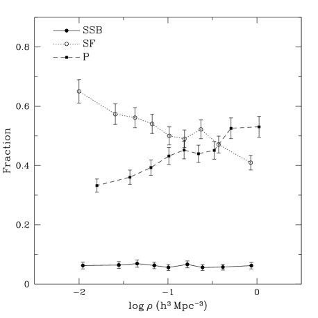
Figure 10: Fraction of galaxies in each spectral class as a function of the local galaxy density. Each density bin contains about the same number of galaxies. The error bars are computed assuming a Poisson statistics.

Figure 11: H$\alpha$ and [O ii] equivalent width distributions as a function of local density of galaxies. The filled circles connected by a solid line represent the median values of each distribution and the error bars are the respective quartiles. Each density bin contains about the same number of galaxies (399).

3.4 Aperture bias

At this point it is convenient to revisit the problem of aperture bias (see 2.4). This effect was not considered in the sample selection nor in the previous analysis. However, it may introduce a redshift dependence in the measured galaxy spectra, since the fraction of galaxy light received by a fiber increases with increasing distance. Zaritsky, Zabludoff & Willick (1995), based on an analysis of LCRS spectra, suggest that for reshifts $z>0.05$ the effect is minimized. This redshift is exactly the upper limit of our sample and, thus, it is necessary to verify whether our results are significantly affected by this bias.

For that, we investigated the behaviour of the EWs of [O ii], H$\delta$, and H$\alpha$ as a function of redshift. We divided the sample in several redshift bins containing the same number of objects, and computed the median value and the quartiles of each spectral indice in each bin. Fig. 12 shows as solid lines the median values of each distribution, as well as their respective quartiles. Each redshift bin contains the same number of objects. Clearly, the median values of the equivalent widths of the three lines analysed here do not show any trend with the redshift, meaning that our measurements seem to be unaffected by the aperture bias.

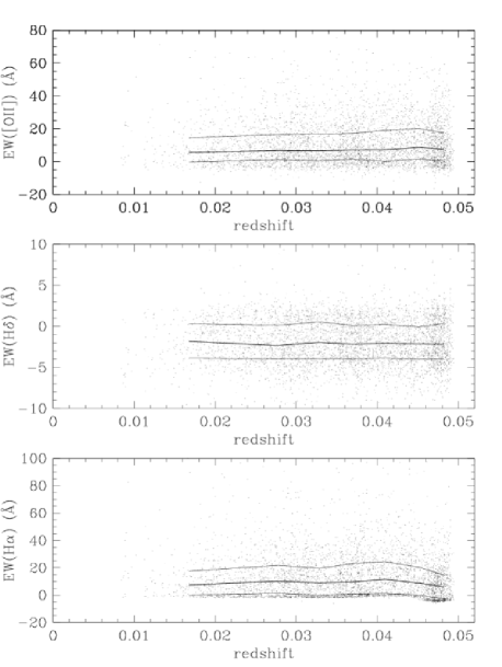
Figure 12: Distribution of EWs as a function of the redshift: a) EW([O ii]), b) EW(H$\delta$), c)EW(H$\alpha$). It is also shown, for each distribution, their median values and the respective quartiles (as solid lines).

4 Discussion

The environmental behaviour of the fractions of SF and P spectral classes, shown in Fig. 10, complements results previously obtained by other authors mainly for the SFR. For example, Balogh et al. (1998, 1999) found that cluster galaxies have lower star-formation rates than field galaxies with similar disk-to-bulge ratio and luminosity. Hashimoto et al. (1998) used the Las Campanas Redshift Survey data to study the relation between local density and star formation in galaxies with same concentration index. Their results show that star-forming galaxies are preferentially found in low-density environments, and the authors point out that the SFR of galaxies with similar structure is sensitive to the local galaxy density. Similar results were also obtained by Carter et al. (2001), using the spectroscopic data from the 15R-North galaxy redshift survey. Here we have considered a sample of field galaxies, showing that the fractions of the P and SF spectral classes vary smoothly with the local density.

Lewis et al. (2002) have used 2dFGRS spectra to investigate the star formation rate of galaxies in different environments around clusters using a parameter $\mu^{*}$ which is proportional to EW(H$\alpha$). They found that there is, indeed, a correlation between SFR and local projected density which is significant only for projected densities above $\sim$ 1 galaxy Mpc^-2 (for galaxies brighter than $M_{b}=-19$, assuming $H_{0}=70$ km s^-1 Mpc^-1), that corresponds approximately to the mean density at the cluster virial radius. Using data from the first release of the SDSS project (Early Data Release, EDR), Gómez et al. (2003) also obtain a relation between SFR and projected density. They show that there is a characteristic break in the SFR distribution at a local projected galaxy density of $\sim 1h^{-2}_{75}$Mpc^-2, corresponding to a clustercentric radius of $\sim$ 3–4 virial radii. Below this density the SFR increases only slightly, whereas at denser regions it is strongly suppressed. Thus, if one assumes that the equivalent width of H$\alpha$, for instance, is proportional to the star formation rate of a galaxy, like assumed by Lewis et al. (2002), our results are similar to those obtained by Gómez et al. (2003) for regions farther than 3 virial radii of cluster cores. Thus, the correlation between the H$\alpha$ and [O ii] equivalent widths and the local density shown in Fig. 11 reinforce the idea that even low-density environments play an important role in stablishing the fraction of passive and/or star forming galaxies.

Our results also show that the fraction of star-forming galaxies varies smoothly along all range of densities covered by our sample, suggesting that the population of galaxies showing evidences of star formation activity seems to be affected by the environment everywhere. This is an important issue that needs to be clarified, because it may provide important hints about the physical mechanisms that are behind the relation between star formation and galaxy environment. Indeed, if only environments with relatively large densities affects star formation, processes that occur mainly in clusters, like ram-pressure stripping or galaxy harassment may be considered the drivers of the trends observed between star formation and environment; on the other hand, if this trend is present for galaxies in clusters as well as for those in the field, as our results support, mechanisms that act everywhere, like tidal interactions, should be playing a relevant role.

At this point it is convenient to discuss the behaviour of SSB galaxies. We have shown in Section 3 that the fraction of these galaxies is essentially independent of their luminosity and local number density, at least for the range of values of these quantities present in our sample. We have also shown that an increase in density tends to decrease the fraction of star-forming galaxies, and then the observed independence of the SSB fraction with $\rho$ is somewhat unexpected. In fact, such a behaviour may be an indication that interactions, either between galaxies, or between a galaxy and its environment, may trigger a starburst in a galaxy. Moss & Whittle (2000) suggest that tidal effects due to gravitational interactions (either galaxy$-$galaxy, galaxy$-$group or galaxy$-$cluster) originate bursts of star formation and morphological distortions in spiral galaxies, with a frequency increasing within high-density environments. Similar results have been reported by Hashimoto & Oemler (2000). Davis et al. (1997), in a study of poor groups of galaxies, also suggest that the interaction of a galaxy with their neighbours increases its star formation rate; however, they point out that morphological peculiarities produced by tidal effects may leave the H i disks more vulnerable to external hydrodynamic forces, turning subsequent gas removal more efficient. Consequently, any star-formation burst in high density environments should be short-lived in this scenario.

In order to verify whether tidal interactions are actually inducing the starbursts that characterize SSB galaxies, we tried to verify whether these galaxies in our sample do show any evidence of morphological distortions. For this, we have examined their images, using the SuperCOSMOS Sky Survey(Hambly et al., 2001). We divided the SSB galaxy sample in two groups containing 50 objects in each one, comprising galaxies located in the bin of lowest galaxy density ($-2.44<\log\rho$ (Mpc^-3 $h^{-3}$)$\,<-1.52$) and in the bin of highest density ($-0.40<\log\rho$ (Mpc^-3 $h^{-3}$)$\,<0.46$), respectively. In low-density regions, the fraction of SSBs showing any kind of peculiarity is $\sim 10$ per cent. When we analyse images of the galaxies in the densest environments, this fraction increases to $\sim 30$ per cent. As a conclusion, although tidal interactions may not be the only mechanism producing the starburst that characterizes SSB galaxies, they are probably having a major role in inducing the large rates of star-formation observed in these objects, even in the low-density regions of the field.

5 SUMMARY AND CONCLUSIONS

In this paper we have investigated the environmental dependence of the population of star-forming galaxies with a volume-limited sample of field galaxies extracted from the final release of the 2dF Redshift Galaxy Survey and containing $4782$ objects. We have adopted a spectral classification that characterizes the star formation through the equivalent widths of [O ii]$\lambda$3727 and H$\delta$. The environment is described by the local spatial density of galaxies. We have then analysed the distribution of fractions for each spectral class as a function of density, mainly, and luminosity. Our main findings are the following:

1. The star-forming galaxies in our sample are mostly low-luminosity objects, whereas brighter objects include mainly passive galaxies that do not present significant activity of star formation. The same behaviour is noted when we analyse the luminosity dependence of star formation indicators like H$\alpha$ and [O ii] equivalent widths: these quantities are higher for low-luminosity objects. The short starburst galaxies (SSB) do not show strong trends with luminosity, except for magnitudes at the faint end of our sample, where their fraction seems to increase.

2. The environmental distribution of spectral classes indicates that star-forming galaxies (SF) and passive galaxies (P) display a distinct behaviour relative to their habitat: the P fraction increases with increasing density; in contrast, the SF fraction decreases with $\rho$. On the other hand, the fraction of SSB galaxies is essentially environment independent, and relative to all star-forming galaxies, the fraction of SSBs increases with increasing density.

3. The smooth relation between the fraction of star-forming galaxies and local density indicates that process affecting star formation activity do act everywhere, suggesting that mechanisms like tidal interactions – that act in all environments – may play a relevant role on the star formation properties of galaxies.

In the hierarchical scenario of galaxy formation, as galaxy clustering evolves, the density around a galaxy tends to increase, in all environments. Higher density probably means more interactions. Our results give support to this broad view, because the fraction of star-forming galaxies seems to be affected by the environment in all range of densities covered by our sample. Thus, there are physical mechanisms that act efficiently on the star formation in all environments, not only in the high-density regions of galaxy clusters.

References

- Abraham et al. (1996) Abraham R.G., Smecker-Hane T.A., Hutchings J.B., Calrberg R.G., 1996, ApJ, 471, 694
- Balogh et al. (1998) Balogh M.L., Schade D., Morris S.L., Yee H.K.C., Carlberg R.G., Ellingson E., 1998, ApJ, 504, L75
- Balogh et al. (1999) Balogh M.L., Morris S.L., Yee H.K.C., Carlberg R.G., Ellingson E., 1999, ApJ, 527, 54
- Barbaro & Poggianti (1997) Barbaro G., Poggianti B.M., 1997, A&A, 324, 490
- Barnes & Hernquist (1991) Barnes J.E., Hernquist L.E., 1991, ApJL, 370, L65
- Bekki (2001) Bekki K., 2001, ApJ, 546, 189
- Bekki, Couch & Shioya (2001) Bekki K., Couch W.J., Shioya Y., 2001, PASJ, 53, 395
- Bekki, Shioya & Couch (2001) Bekki K., Shioya Y., Couch W.J., 2001, ApJ, 547, L17
- Biviano et al. (1997) Biviano A., Katgert P., Mazure A., Moles M., den Hartog R., Perea J., Focardi P., 1997, A&A, 321, 84
- Bothun & Dressler (1986) Bothun G.D., Dressler A., 1986, ApJ, 301, 57
- Bravo-Alfaro et al. (2000) Bravo-Alfaro H., Cayatte V., van Gorkon J.H., Balkowski C., 2000, AJ, 119, 580
- Bromley et al. (1998) Bromley B.C., Press W.H., Lin H., Kirshner R.P., 1998, ApJ, 505, 25
- Byrd & Valtonen (1990) Byrd G., Valtonen M., 1990, ApJ, 350, 89
- Carter et al. (2001) Carter B.J., Fabricant D.G., Geller M.J., Kurtz M.J., 2001, ApJ, 559, 606
- Casertano & Hut (1985) Casertano S., Hut P., 1985, ApJ, 298, 80
- Cid Fernandes et al. (2001) Cid Fernandes R., Sodré L., Schmitt H.R., Leão J.R.S., 2001, MNRAS, 325, 60
- Colless et al. (2001) Colless M., et al. (The 2dFGRS Team), 2001, MNRAS, 328, 1039
- Colless et al. (2003) Colless M., et al. (The 2dFGRS Team), 2003, astro-ph/0306581
- Cuevas (2000) Cuevas H., 2000, PhD thesis, University of S o Paulo
- Davis et al. (1997) Davis D.S, Keel W.C., Mulchaey J.S., Henning P.A., 1997, AJ, 114, 613
- De Propris et al. (2002) De Propris R., et al. (The 2dFGRS Team), 2002, MNRAS, 329, 87
- Dressler & Gunn (1983) Dressler A., Gunn J.E., 1983, ApJ, 270, 7
- Dressler, Thompson & Shectman (1985) Dressler A., Thompson I.B., Shectman S.A., 1985, ApJ, 288, 481
- Ellingson et al. (2001) Ellingson E., Lin H., Yee H.K.C., Carlberg R.G., 2001, ApJ, 547, 609
- Folkes et al. (1999) Folkes S., et al. (The 2dFGRS Team), 1999, MNRAS, 308, 459
- Fujita & Nagashima (1999) Fujita Y., Nagashima M., 1999, ApJ, 516, 619
- Fukugita et al. (1996) Fukugita M., Ichikawa T., Gunn J.E., Doi M., Shimasaku K., Schneider D.P., 1996, AJ, 111, 1748
- Fukunaga (1990) Fukunaga K., 1990, Introduction to Statistical Pattern Recognition, 2nd edn. Academic Press
- Gallagher, Hunter & Bushouse (1989) Gallagher J.S., Hunter D.A., Bushouse H., 1989, AJ, 97, 700
- Gavazzi et al. (1998) Gavazzi G., Catinella B., Carrasco L., Boselli A., Contursi A., 1998, AJ, 115, 1745
- Gavazzi & Jaffe (1985) Gavazzi G., Jaffe W., 1985, ApJ, 294, L89
- Giovanelli & Haynes (1985) Giovanelli R., Haynes M.P., 1985, ApJ, 292, 404
- Girardi et al. (1998) Girardi, M., Giuricin, G., Mardirossian, F., Mezzetti, M., Boschin, W., 1998, ApJ, 505, 74
- Gisler (1978) Gisler G.R., 1978, MNRAS, 183, 633
- Gómez et al. (2003) Gómez P.L., et al., 2003, ApJ, 584, 210
- Goto et al. (2003) Goto T. et al., 2003, PASJ, 55, 757
- Gunn & Gott (1972) Gunn J.E., Gott J.R., 1972, ApJ, 176, 1
- Hambly et al. (2001) Hambly N.C., MacGillivray H.T., Read M.A., et al., 2001, MNRAS, 326, 1279
- Hamilton (1985) Hamilton D., 1985, ApJ, 297, 371
- Hashimoto et al. (1998) Hashimoto Y., Oemler A., Lin H., Tucker D.L., 1998, ApJ, 499, 589
- Hashimoto & Oemler (2000) Hashimoto Y., Oemler A., 2000, ApJ, 530, 652
- Kennicutt (1983) Kennicutt R.C., 1983, ApJ, 272, 54
- Kennicutt & Kent (1983) Kennicutt R.C., Kent, S.M., 1983, AJ, 88, 1094
- Kennicutt (1992) Kennicutt R.C., 1992, ApJ, 388, 310
- Kenney & Young (1989) Kenney J.D.P., Young J.S., 1989, ApJ, 344, 171
- Kochanek, Pahre & Falco (2000) Kochanek C.S., Pahre M.A., Falco E.E., 2000, submitted (astro-ph/0011458)
- Larson, Tinsley & Caldwell (1980) Larson R.B., Tinsley B.M., Caldwell C.N., 1980, ApJ, 237, 692
- Lavery & Henry (1994) Lavery R.J., Henry J.P., 1994, ApJ, 426, 524
- Lewis et al. (2002) Lewis I., et al. (The 2dFGRS Team), 2002, MNRAS, 334, 673
- Lin et al. (1996) Lin H., Kirshner R.P., Shectman S.A., Landy S.D., Oemler A., Tucker D., Schechter P.L., 1996, ApJ, 464, 60
- Loveday, Tresse & Maddox (1999) Loveday J., Tresse L., Maddox S., 1999, MNRAS, 310, 281
- Madgwick et al. (2002) Madgwick D., et al. (The 2dFGRS Team), 2002, MNRAS, 333, 133
- Marzke et al. (1998) Marzke R.O., da Costa L.N., 1997, AJ, 113, 185
- Moss & Whittle (1993) Moss C., Whittle M., 1993, ApJ, 407, L17
- Moss & Whittle (2000) Moss C., Whittle M., 2000, MNRAS, 317, 667
- Norberg et al. (2001) Norberg P., et al. (The 2dFGRS Team), 2001, MNRAS, 328, 64
- Norberg et al. (2002) Norberg P., et al. (The 2dFGRS Team), 2002, MNRAS, 332, 827
- Osterbrock (1960) Osterbrock D.E., 1960, ApJ, 132, 325
- Poggianti et al. (1999) Poggianti B.M., Smail I., Dressler A., Couch W.J., Barger A.J., Butcher H., Ellis R.S., Oemler A., 1999, ApJ, 518, 576
- Poggianti, Bressan & Fransceschini (2001) Poggianti B.M., Bressan A., Franceschini A., 2001, ApJ, 550, 195
- Press et al. (1992) Press, W.H., Teukolsky, S.A., Vetterling, W.T., Flannery, B.P., 1992, Numerical recipes in FORTRAN. The art of scientific computing (Cambridge: University Press)
- Solanes et al. (1996) Solanes J.M., Giovanelli R., Haynes M.P., 1996, ApJ, 461, 609
- Stasińska & Sodré (2001) Stasińska G., Sodré L., 2001, A&A, 374, 919
- Tresse et al. (1999) Tresse L., Maddox S., Loveday J., Singleton C., 1999, MNRAS, 310, 262
- Veilleux & Osterbrock (1987) Veilleux S., Osterbrock D.E., 1987, ApJS, 63, 295
- Vollmer et al. (2001) Vollmer B., Cayatte V., Balkowski C., Duschl W.J., 2001, ApJ, 561, 708
- Zaritsky, Zabludoff & Willick (1995) Zaritsky D., Zabludoff A.I., Willick J.A., 1995, AJ, 110, 1602
- Zucca et al. (1997) Zucca E., et al., 1997, A&A, 326, 477