Conservation Laws in Smooth Particle Hydrodynamics: the DEVA Code

Abstract

We describe DEVA, a multistep AP3M-like-SPH code particularly designed to study galaxy formation and evolution in connection with the global cosmological model. This code uses a formulation of SPH equations which ensures both energy and entropy conservation by including the so-called ${\mathbf{\nabla}}h$ terms. Particular attention has also been paid to angular momentum conservation and to the accuracy of our code. We find that, in order to avoid unphysical solutions, our code requires that cooling processes must be implemented in a non-multistep way.

We detail various cosmological simulations which have been performed to test our code and also to study the influence of the ${\mathbf{\nabla}}h$ terms. Our results indicate that such correction terms have a non-negligible effect on some cosmological simulations, especially on high density regions associated either to shock fronts or central cores of collapsed objects. Moreover, they suggest that codes paying a particular attention to the implementation of conservation laws of physics at the scales of interest, can attain good accuracy levels in conservation laws with limited computational resources.

1 Introduction

In the last few years most cosmological parameters have been determined up to a few percent. The values of $\Omega_{\rm tot}$, $\Omega_{\Lambda}$, $\Omega_{\rm baryon}$ and $H_{0}$ can now be constrained with an unprecedent degree of accuracy (see, for example, Lahav, 2002; Lahav et al., 2002; Netterfield et al., 2002; Spergel et al., 2003, and references therein). The next challenge to cosmologists is to test the predictions of cosmological models at a few hundred kpc scales. It turns out that these are just the relevant scales involved in galaxy formation and evolution. Galaxy formation and evolution are intriguing open questions whose resolution in connection with the global cosmological model will very likely advance considerably in this decade. Even though the field is at its beginnings, the use of numerical methods to study how galaxies are assembled within a cosmological scenario from the field of primordial fluctuations, seems a convenient approach. The main advantage of these approaches (i.e., self-consistent hydrodynamical simulations), is that the physics is introduced at a very general level, and the system evolves as a consequence. We can follow the evolution of the dynamical and hydrodynamical properties of matter in the Universe; galaxy-like objects (GLOs) appear as a consequence of this evolution. And, so, the building-up of objects (cosmic network structure formation at high $z$, collapse, interactions, mergers, accretions), as well as their hydrodynamical consequences (instabilities, gas infall from halos to discs at hundred of kpc scales, gas inflow along discs at tens of kpc scales, shocks, cooling, piling-up of gas necessary for star formation), can be accurately followed. We get not only the properties of objects at any $z$, but also an insight into the physical processes responsible for their formation and evolution. Moreover, numerical hydrodynamical simulations using particles permit very convenient comparisons of GLOs that form in simulations with observational data. Simulations directly provide us, at each $z$, with the structural and dynamical properties of each individual GLO (position and velocity of each of its particles, gas density and temperature of each of its baryonic constituents) and with their individual star formation rates histories (SFRHs). Chemical abundance and spectrophotometrical data are the current standard to compare models of galaxy formation. It is expected that the next generation of astronomical facilities will make possible a new science: mass measurements for distant galaxies (see, for example Verheijen, Bershady & Andersen, 2002). GLOs formed in numerical simulations are particularly suited to be compared to this new kind of data.

Pre-prepared numerical experiments are adequate to describe in detail a particular phase of the formation or evolution of galaxies (for example, merger events or orbital motions of satellites within halos), from initial conditions set by the experimenter. These initial conditions try to model conditions that would have arisen along the evolution of the systems under consideration. They are useful to study basic aspects of the physical processes relevant to evolution. For example, the works by Barnes, Hernquist and Mihos (Barnes, 1989; Barnes & Hernquist, 1991; Barnes, 1992; Barnes & Hernquist, 1992; Mihos & Hernquist, 1994, 1996), which have fundamental importance to understand the role played by mergers in galaxy evolution, have been carried out with this technique. However, in pre-prepared simulations, contrary to the self-consistent approach, the process under consideration is studied in isolation, and not in connection with the other relevant processes involved in galaxy formation and evolution (already mentioned) that, moreover, could interact among themselves in a non-trivial way.

These considerations stress the ability of self-consistent hydrodynamical simulations as a tool to learn how galaxies form from the field of primordial fluctuations and evolve into the objects we observe today. To properly handle this problem, a numerical code has to allow for enough mass, time and space resolution as well as a convenient dynamical range. They should be as fast as possible and with memory requirements within the current computer capabilities. A very important issue when designing a numerical code to study galaxy formation and evolution, is to make sure that conservation laws are accurately verified, and, particularly, i), that angular momentum is conserved at the scales relevant to disc formation; otherwise, galaxy disc formation could meet with some difficulties; and, ii), that entropy is conserved in reversible adiabatic processes, because the violation of this physical principle could produce spurious effects at galaxy scales. By the moment, star formation (SF) processes have to be modelled, either inspired in kpc or pc scale hydrodynamical simulations (Padoan et al., 1999; Avila-Reese & Vázquez-Semadeni, 2001; Vázquez-Semadeni et al., 2000; Wada & Norman, 2001; Kritsuk & Norman, 2002) or other considerations (Katz, 1992; Tissera, Lambas & Abadi, 1997; Kennicutt, 1998; Yepes el al., 1997; Silk, 2001; Springel & Hernquist, 2002b; Elmegreen, 2003; Padoan et al., 2003).

The first choice to be made when designing this kind of codes is the gravity solver. Among current numerical methods, those that employ adaptive techniques in regions of high density, either from a Lagrangian (as AP3M, Couchman, 1991; Couchman, Thomas, & Pearce, 1995) or Eulerian (as the ART and MLAPM codes, Kravtsov, Klypin & Khokhlov, 1997; Knebe, Green & Binney, 2001) approach, are the most suitable to meet the requirements of resolution and large dynamical range, accuracy and rapidity. A detailed comparison between AP3M and ART codes has been carried out by Knebe et al. (2000). They have found out that these codes produce results that are consistent within a 10%, provided that $N_{\rm steps}/DR\geq 2$ ($N_{\rm steps}$ is the number of integration steps; $DR$ stands for the dynamical range). The choice of the gravity solver in a cosmological simulation depends on its purpose. To study galaxy formation and evolution, Lagrangian codes have the advantage over Eulerian codes that they permit to go backwards and forwards in time in a very easy way. For example, the constituent particles of a given object can be identified at a given redshift, $z_{1}$, and one can then analyze their positions in phase space and the properties of the objects or structures they form at a different redshift, $z_{2}$. This is a very convenient method to study evolutionary processes and it motivates our choice of an AP3M-based method as gravity solver for our simulations.

To solve the hydrodynamical equations (and, in general, any hyperbolic system of equations in partial derivatives), there are also two basic different techniques: i), Eulerian methods, and, ii), Lagrangian methods. Eulerian methods are based on the so-called Godunov algorithm (Godunov, 1959). Their new formulations, using adaptive mesh refinements (Norman & Bryan, 1998; Klein et al., 1998; Teyssier, 2002), are particularly well suited to combine with ART-like codes when both gravitational and hydrodynamical forces are considered. For a comparison of the performances of a number of hydrodynamical codes of both kinds see (Kang et al., 1994; Frenk et al., 1999).

Most of the lagrangian methods used in astrophysics are based on the SPH (Smooth Particle Hydrodynamics) technique (Lucy, 1977; Gingold & Monaghan, 1977; Monaghan, 1992). Given the convenience of this technique to be applied to cosmological simulations, a number of authors developed SPH codes to be used in a cosmological context. Some of them follow. Evrard (1988) first used SPH techniques in cosmological simulations (a P3M-SPH code). Hernquist & Katz (1989); Katz, Weinberg, & Hernquist (1996), as well as Navarro & White (1993), coupled a SPH code to the Barnes & Hut (1986) Tree algorithm. Vedel, Hellsten & Sommer-Larsen (1999) modelled their TREESPH code after Hernquist & Katz (1989) and Davé, Dubinski, & Hernquist (1997) introduced a parallel version of this code, while Steinmetz (1996) makes use of a special purpose hardware to compute the gravitational forces by direct summation (GRAPE). Serna, Alimi, & Chièze (1996) coupled SPH with a PP algorithm in a code designed to be run on a Connection Machine, and Alimi et al. (2002) incorporated in a Tree-SPH code the so-called ${\mathbf{\nabla}}h$ terms (see below). GADGET (Springel, Yoshida & White, 2001) uses either a Tree scheme or GRAPE, with individual integration timesteps, and both, serial and parallel versions. Another parallel Tree-Sph code is GASOLINE (Borgani et al., 2002).

As already mentioned, AP3M-based codes are particularly well suited to study galaxy formation through self-consistent cosmological simulations. The first AP3M-SPH code was introduced by Couchman, Thomas, & Pearce (1995) (Hydra code, see also Pearce & Couchman, 1997). Tissera, Lambas & Abadi (1997) carried out a second implementation. In these implementations, the integration timestep is global (i.e., at a given time, the same for all particles). In cosmological simulations, however, multiple time scales appear, due to their very large dynamical ranges from very dense volumes to very rarefied zones. To get an accurate enough integration scheme, and, at the same time, to avoid that particles in denser volumes slow down the simulations, it is advantageous to introduce individual integration timesteps, i.e., at each time, different timesteps for each particle, depending on the density of the region it samples. This is the optimal design of the code to increase the mass resolution.

Another shortcoming of conventional SPH formulations concerns the entropy violation of the dynamical equations, related to the space dependence of the smoothing length of SPH particles, $h(r,t)$, as noted by some authors (Hernquist, 1993; Nelson & Papaloizou, 1993, 1994; Serna, Alimi, & Chièze, 1996). A rigorous formulation of SPH requires that additional terms must be included in the particle equations of motion which account for the variability of $h$, usually termed as “the ${\mathbf{\nabla}}h$ terms”. Until very recently, they were considered as having a negligible effect on the global dynamics of systems (Gingold & Monaghan, 1982; Evrard, 1988) and, therefore, SPH codes ignored such additional terms and focused on energy conservation. Alternatively, treatments of hydrodynamics based on the Lagrange equations can be formulated that are well behaved in their conservation properties of both, energy and entropy, as that introduced recently by Springel & Hernquist (2002a). The effects of entropy violation in SPH codes are not completely clear and they need to be analyzed in much more detail, specially in simulations where galaxies are formed in a cosmological framework. Previous works have analyzed this question in the case of the collapse of isolated objects and have found that, if such correction terms are neglected, the density peaks associated to central cores or shock fronts are overestimated at a $\simeq$30$\%$ level (Alimi et al., 2002).

To make up for these shortcomings when dealing with problems related to galaxy formation and evolution, we introduce a new code, DEVA, where gravity is solved by means of an AP3M-like technique, and hydrodynamics with a SPH technique, with individual integration timesteps. The space dependence of the SPH resolution scale, $h(r,t)$, has been taken into account, in order to ensure the conservative character of the equations of motion, as long as entropy and energy is considered. Another important particularity of DEVA is the attention paid to angular momentum conservation, a key point to enable disc formation in simulations (Domínguez-Tenreiro, Tissera & Sáiz, 1998; Sáiz et al., 2001, and references therein). Our choice has been to put the stress into conservation laws rather than into saving CPU time. But saving CPU time has also been one of our concerns, so that the code is fast enough that cosmological self-consistent simulations can be run on a modest computer machine.

The paper is organized as follows: $\S$1 is the Introduction. In $\S$2, the SPH method is briefly reviewed and we present the SPH equations when the ${\mathbf{\nabla}}h$ terms are considered. $\S$ 3 is devoted to the particularities of the DEVA code, and $\S$ 4 to test whether the code integrates correctly the hydrodynamical and N-body equations (standard tests). In $\S$ 5 we introduce some self-consistent simulations run with DEVA, compare to one standard of reference for hydrodynamical simulations in a cosmological framework (the Santa Barbara cluster comparison project Frenk et al., 1999), and analyze the effects of the ${\mathbf{\nabla}}h$ terms in these simulations. Finally, in $\S$ 6, we give a summary of the work and discuss DEVA performances.

2 The SPH Method

2.1 Kernel estimates

The basic idea of the SPH method (Lucy, 1977; Gingold & Monaghan, 1977) lies in representing the fluid elements by $N_{g}$ particles which act as interpolation centers to determine the local value of any macroscopic variable $f(\mbox{\it{\bf r}})$. In order to smooth out local statistical fluctuations, this interpolation is performed by convolving the field $f(\mbox{\it{\bf r}})$ with a smoothing (or kernel) function $W$. For example, the smoothed estimate of the local density is

$$\rho(\mbox{\it{\bf r}}_{i})=\sum_{j=1}^{N_{g}}m_{j}W(r_{ij},h_{i},h_{j})\;,$$ (1)

where $r_{ij}=\mid\mbox{\it{\bf r}}_{i}-\mbox{\it{\bf r}}_{j}\mid$, $m_{j}$ is the mass of particle $j$, and $h_{k}$ is the smoothing length for particle $k$, which specifies the size of the averaging volume.

Ideally, the individual particle smoothing lengths $h_{k}$ must be updated so that each particle has a constant number of neighbors $N_{S}$. By neighbors we mean those particles $j$ with distances $r_{kj}\leq 2h_{k}$. Such a condition can be exactly implemented by constructing, for each particle $k$, a list of its $N_{S}$ nearest neighbors. The smoothing length of $k$ is then defined to be

$$h_{k}=\frac{1}{2}\mid\mbox{\it{\bf r}}_{k}-\mbox{\it{\bf r}}_{k_{f}}\mid\;,$$ (2)

where $\mbox{\it{\bf r}}_{k_{f}}$ is the position vector of particle $k$’s most distant neighbor. Since each particle has its own $h$ value, it is possible to find couples of particles $(j,k)$ such that $j$ is a neighbor of $k$, but $k$ is not a neighbor of $j$. In these cases, it is obvious that the reciprocity principle is not satisfied and, therefore, simulations will not conserve momentum. In order to solve this problem, it is necessary to symmetrize the SPH equations by using, for example, averaged kernels (Hernquist & Katz, 1989):

$$W_{ij}\equiv W(r_{ij},h_{i},h_{j})=\frac{1}{2}\left[W(r_{ij},h_{i})+W(r_{ij},h_{j})\right]\;.$$ (3)

A first consequence of the adopted symmetrization procedure is the specific form for the kernel derivatives. As a matter of fact, Eq. (3) implies that $W_{ij}$ is a function of three variables: $r_{ij}$, $h_{i}$ and $h_{j}$. Consequently, its gradient ${\mathbf{\nabla}}_{i}W_{jk}$ is given by:

$${\mathbf{\nabla}}_{i}W_{jk}=\frac{1}{2}\left[\left(\frac{\partial W(r_{jk},h_{j})}{\partial r_{jk}}+\frac{\partial W(r_{jk},h_{k})}{\partial r_{jk}}\right){\mathbf{\nabla}}_{i}r_{jk}\right]$$

$$+\frac{1}{2}\left[\frac{\partial W(r_{jk},h_{j})}{\partial h_{j}}{\mathbf{\nabla}}_{i}h_{j}+\frac{\partial W(r_{jk},h_{k})}{\partial h_{k}}{\mathbf{\nabla}}_{i}h_{k}\right]$$ (4)

The first part of Eq. (2.1), which does not involve derivatives of the smoothing lengths, is the usual symmetrized form of ${\mathbf{\nabla}}_{i}W_{jk}$. The second part, which involves derivatives of the smoothing lengths, arises because of the spatial and temporal variability of $h$. We shall refer to terms of this type as ’${\mathbf{\nabla}}h$ terms’. Most implementations of the SPH algorithm consider only the first one and neglect the ${\mathbf{\nabla}}h$ terms.

2.2 Hydrodynamic equations

The motion of particle $i$ is determined by the momentum and energy equations:

$$\frac{d\mbox{\it{\bf v}}_{i}}{dt} = \textbf{a}_{i}^{P}+\textbf{a}_{i}^{visc}-{\mathbf{\nabla}}\Phi_{i}$$ (5)

$$\frac{du_{i}}{dt} = \frac{P_{i}}{\rho_{i}^{2}}\frac{d\rho_{i}}{dt}+{\cal{H}}_{i}\;,$$ (6)

where $\Phi_{i}$ is the local gravitational potential, $\textbf{a}_{i}^{P}$ is the acceleration due to pressure forces, $\textbf{a}_{i}^{visc}$ is the acceleration due to viscosity forces, $u$ is the specific internal energy, $P=(\gamma-1)\rho u$ is the pressure (with $\gamma$ being the constant heat ratio), and ${\cal{H}}_{i}$ is the power due to non-adiabatic heating or cooling processes.

A fully consistent SPH expression for pressure forces, satisfying all conservations laws (including entropy conservation in reversible adiabatic problems), was obtained by Nelson & Papaloizou (1993, 1994):

$${\bf F}_{i}^{P}=-\sum_{j}m_{j}\frac{P_{j}}{\rho_{i}^{2}}{\mathbf{\nabla}}_{i}\rho_{j}\;.$$ (7)

Using Eqs. (1) and (2.1) to compute ${\mathbf{\nabla}}_{i}\rho_{j}$, one obtains

$${\bf a}_{i}^{P} = -\sum_{j}m_{j}\left(\frac{P_{i}}{\rho_{i}^{2}}+\frac{P_{j}}{\rho_{j}^{2}}\right)\left[\frac{\partial W(r_{ij},h_{i},h_{f})}{\partial r_{ij}}\right]\frac{\mbox{\it{\bf r}}_{ij}}{r_{ij}}$$

$$- \frac{1}{4}\tilde{r}_{i}\sum_{j}m_{j}\left(\frac{P_{i}}{\rho_{i}^{2}}+\frac{P_{j}}{\rho_{j}^{2}}\right)\frac{\partial W(r_{ij},h_{i})}{\partial h_{i}}$$

$$+ \frac{1}{4}\sum_{j}\tilde{r_{j}}\delta_{ij_{f}}\sum_{k}\frac{m_{j}m_{k}}{m_{i}}\left(\frac{P_{j}}{\rho_{j}^{2}}+\frac{P_{k}}{\rho_{k}^{2}}\right)\frac{\partial W(r_{jk},h_{j})}{\partial h_{j}}\;,$$

where $\tilde{r}_{k}\equiv\mbox{\it{\bf r}}_{kk_{f}}/r_{kk_{f}}$.

On the other hand, using Eqs. (1) and (2.1) to compute the $d\rho_{i}/dt$ derivative appearing in Eq. (6), the energy equation becomes:

$$\frac{du_{i}}{dt} = \frac{P_{i}}{\rho_{i}^{2}}\sum_{j}m_{k}\left[\frac{\partial W(r_{ij},h_{i},h_{j})}{\partial r_{ij}}\right]\frac{\textbf{r}_{ij}\cdot\textbf{v}_{ij}}{r_{ij}}$$ (9)

$$+ \frac{1}{4}\frac{P_{i}}{\rho_{i}^{2}}\sum_{j}m_{j}\left[\frac{\partial W(r_{ij},h_{i})}{\partial h_{i}}\breve{r}_{i}+\frac{\partial W(r_{ij},h_{j})}{\partial h_{j}}\breve{r}_{j}\right]+{\cal{H}}_{i}\;,$$

where

$$\breve{r}_{k}\equiv\frac{\textbf{r}_{kk_{f}}\cdot\textbf{v}_{kk_{f}}}{r_{kk_{f}}}\;.$$ (10)

Note that Eqs. (2.2) and (9) have been deduced by using both spatial and time derivatives of the SPH density as defined by Eq. (1) with the symmetrization specified in Eq. (3), because compatibility with the conservation laws requires that the SPH force and energy equations are evaluated in consistency with the density definition. In the case of DEVA, this requirement increases the CPU time per integration step. In fact, since the density $\rho_{i}$ associated to a particle $i$ depends on both $h_{i}$ and $h_{j}$, for $j=1,...,N_{S}$, (i.e., for its $N_{S}$ nearest neighbors, see Eq. 1), the computation of $\rho_{i}$ at a given integration step requires the knowledge of $h_{j}$ for these $N_{S}$ nearest neighbors at its beginning . This can be achieved either by using the $h_{j}$ values predicted in the previous integration step or by performing, at each step, a first loop over the particles to compute their $h_{j}$ values and, once it is over, a second loop to compute their hydrodynamical properties. Since we look for a high accuracy rather than a high computational speed, we have adopted this latter possibility.

As usual in SPH, to account for dissipation at shocks, the above equations must be completed by adding an artificial viscous pressure term, $\Pi_{ij}$. When the ${\mathbf{\nabla}}h$ terms are considered, $\Pi_{ij}$ is added only to the leading term of equations (2.2) and (9), that is, those not involving ${\mathbf{\nabla}}h$ terms (Nelson & Papaloizou, 1994):

$$\frac{P_{i}}{\rho_{i}^{2}}\rightarrow\frac{P_{i}}{\rho_{i}^{2}}+\frac{\Pi_{ij}}{2},\qquad\frac{P_{i}}{\rho_{i}^{2}}+\frac{P_{j}}{\rho_{j}^{2}}\rightarrow\Pi_{ij}\;,$$ (11)

where we have adopted the standard viscous pressure proposed by Monaghan & Gingold (1983):

$$\Pi_{ij}=\frac{-\alpha\mu_{ij}\overline{c}_{ij}+\beta\mu_{ij}^{2}}{\overline{\rho}_{ij}}\;,$$ (12)

where $\alpha$ and $\beta$ are constant parameters of order unity, $\eta^{2}$ is a softening parameter to prevent numerical divergences, $c_{i}$ is the local sound speed, and

$$\mu_{ij}=\left\{\begin{array}[]{ll}\frac{\mbox{\it{\bf v}}_{ij}\mbox{\it{\bf r}}_{ij}}{{\normalsize h_{ij}\left(r^{2}_{ij}/h_{ij}^{2}+\eta^{2}\right)}}&\mbox{\it{\bf v}}_{ij}\mbox{\it{\bf r}}_{ij}<0\\ 0&\mbox{\it{\bf v}}_{ij}\mbox{\it{\bf r}}_{ij}\geq 0\end{array}\right.\;.$$ (13)

3 The DEVA code

The simulation of a system constituted by $N$ particles usually requires a computational effort which considerably varies from some regions (or particles) to other. For example, regions of high density and submitted to strong shocks need to be simulated with timesteps much shorter than the rest of the system. In the AP3M+SPH codes described in the literature, all the particles in the system are simultaneously advanced at each timestep. The particle needing the highest time resolution determines the timestep length of all the others. Consequently, some few particles can slow down the simulation of a system. To make a code more efficient in handling with problems with multiple time scales, the computational effort must be centered on those particles that require it, avoiding useless computations for the remaining particles. In other words, it is necessary to allow for different timesteps for each particle.

3.1 AP3M with individual timesteps

A PEC (Predict-Evaluate-Correct) scheme with individual timesteps has been developed and implemented on our code in the following way:

1. We enter the step $n$ (which corresponds to the time $t^{n}$) with known positions $\mbox{\it{\bf r}}_{i}^{n}$, velocities $\mbox{\it{\bf v}}_{i}^{n}$, and accelerations $\mbox{\it{\bf a}}_{i}^{n}$, for all the $N$ particles. Furthermore, any integration scheme with individual timesteps needs some information to identify, at each step, those particles needing a recomputation of their acceleration. This information is stored in two vectors $t_{i}^{last}$ and $t_{i}^{next}$, where $t_{i}^{last}$ is the time at which the last update of $\mbox{\it{\bf a}}_{i}$ was performed, while $t_{i}^{next}=t_{i}^{last}+\Delta t_{i}$ is the time at which a recomputation of $\mbox{\it{\bf a}}_{i}$ will be necessary in the future.

   $$\mbox{\it{\bf r}}_{i}^{n},\mbox{\it{\bf v}}_{i}^{n},\mbox{\it{\bf a}}_{i}^{n},t_{i}^{next},t_{i}^{last}$$ (14)

2. A list is constructed with those particles $j$ which will be advanced at the current step. Such particles are labelled as active. Obviously, the particle $j_{min}$ with the smallest prediction time, $t_{j}^{next}-t^{n}$, must be included in this list, and fixes the timestep of the remaining active particles:

   $$\Delta t=\min_{j}(t_{j}^{next}-t^{n})\;.$$ (15)

   Since each step requires the update of many auxiliary arrays, it is impractical to advance only a single particle. For this reason, we label as active all particles within a cubic box around $j_{min}$. The size of the activation box is chosen, at each position, so that it contains a small fraction of the total number of particles.

3. For all particles, active or not, we predict the value of $\mbox{\it{\bf r}}^{n+1}$ and $\mbox{\it{\bf v}}^{n+1}$ at $t^{n+1}$

   $$\tilde{\mbox{\it{\bf r}}}_{i}^{n+1} = \mbox{\it{\bf r}}_{i}^{n}+\mbox{\it{\bf v}}_{i}^{n}\Delta t+\mbox{\it{\bf a}}_{i}^{n}(\Delta t)^{2}/2$$ (16)

   $$\tilde{\mbox{\it{\bf v}}}_{i}^{n+1} = \mbox{\it{\bf v}}_{i}^{n}+\mbox{\it{\bf a}}_{i}^{n}\Delta t\;.$$ (17)

4. Only for active particles, we compute their accelerations and correct $\mbox{\it{\bf r}}^{n+1}$ and $\mbox{\it{\bf v}}^{n+1}$ using :

   $$\mbox{\it{\bf r}}_{j}^{n+1} = \tilde{\mbox{\it{\bf r}}}_{i}^{n+1}+A(\mbox{\it{\bf a}}_{j}^{n+1}-\mbox{\it{\bf a}}_{j}^{n})(\delta t_{j})^{2}/2$$ (18)

   $$\mbox{\it{\bf v}}_{j}^{n+1} = \tilde{\mbox{\it{\bf v}}}_{i}^{n+1}+B(\mbox{\it{\bf a}}_{j}^{n+1}-\mbox{\it{\bf a}}_{j}^{n})(\delta t_{j})\;,$$ (19)

   where the choice $A=1/3$ and $B=1/2$ maintains accuracy to second order both in positions and velocities. In these expressions, $\delta t_{j}$ represents the time interval elapsed from the last evaluation of $\mbox{\it{\bf a}}_{j}$ to that performed in the current timestep

   $$\delta t_{j}=t^{n}+\Delta t-t_{j}^{last}\;.$$ (20)

   Note that, unlike $\Delta t$, the $\delta t_{j}$ value is different for each active particle.

5. We update the global time $t^{n+1}=t^{n}+\Delta t$, as well as the $t_{j}^{last}$ and $t_{j}^{next}$ values of each active particle. Here, in order to maintain the numerical stability of the AP3M algorithm, the individual timestep $\Delta t_{j}$ must be smaller than the time scale for significant displacements or changes in velocity due to accelerations:

   $$\Delta t_{i}^{a}=(\epsilon^{2}/{a_{i}^{2}})^{1/4}\;,$$ (21)

   where $\epsilon$ is the gravitational softening.

3.2 Including SPH

The above integration scheme may easily be extended to include hydrodynamics. The SPH processes involve three new independent variables in addition to those listed in Eq. (14):

$$h_{j}^{n},u_{j}^{n},\dot{u}_{j}^{n}\;,$$ (22)

where $h_{j}^{n}$ is the smoothing length, $u_{j}^{n}$ the specific internal energy, and $\dot{u}_{j}^{n}$ its derivative. For all particles, we must then predict the value of $u_{j}^{n+1}$ at $t^{n+1}$

$$\tilde{u}_{j}^{n+1}=u_{j}^{n}+\dot{u}_{j}^{n}\Delta t\;,$$ (23)

and compute, for active particles, both their total acceleration ($\mbox{\it{\bf a}}_{grav}^{n}$ and $\mbox{\it{\bf a}}_{hydro}^{n}$) as well as their hydrodynamical variables ($h^{n+1}$, $\rho^{n+1}$, $P^{n+1}$ and $\dot{u}_{i}^{n}$). These quantities are then used to correct the internal energy of active particles:

$$u_{j}^{n+1}=\tilde{u}_{j}^{n+1}+C(\dot{u}_{j}^{n+1}-\dot{u}_{j}^{n})(\delta t_{j})\;,$$ (24)

where the choice $C=1/2$ maintains accuracy to second order in internal energies.

Now, the numerical stability requires additional limits on the timestep of each gas particle. A first timestep control is that concerning the time scale for significant displacements or changes in velocity due to accelerations:

$$\Delta t_{i}^{a}=(h_{i}^{2}/{a_{i}^{2}})^{1/4}\;.$$ (25)

A second limit on $\Delta t_{i}$ is usually given by a timestep control which combines the Courant and the viscous conditions:

$$\Delta t_{i}^{cv}=\left[\frac{h_{i}}{c_{i}+1.2(\alpha c_{i}+\beta\max_{j}\mid\!\mu_{ij}\!\mid)}\right]\;.$$ (26)

When required, radiative cooling is implemented in an integral form (Thomas, & Couchman, 1992) using the fact that, due to the Courant condition, the density field is nearly constant over a time-step:

$$\int_{u_{i}}^{u_{i}-\Delta u_{i}^{cool}}\frac{du_{i}^{cool}}{\Lambda}=-\frac{\Delta t}{\rho_{i}}\;,$$ (27)

where $\Lambda(T,\rho)$ is the power radiated per unit volume and $\Delta u_{i}^{cool}$ is the change in $u_{i}$ due to cooling processes.

This integral procedure circumvents the need of a control time for cooling, and, hence, it never limits the timestep. The numerical stability of our code requires that cooling effects must be updated at each step for all particles, active or not. Otherwise, the simultaneous presence of already cooled and not yet cooled particles in a given object would break the local pressure equilibrium and, as a result, cold particles would fall to the object center causing a non-physical core of very high density (see $\S$5.2 for an example).

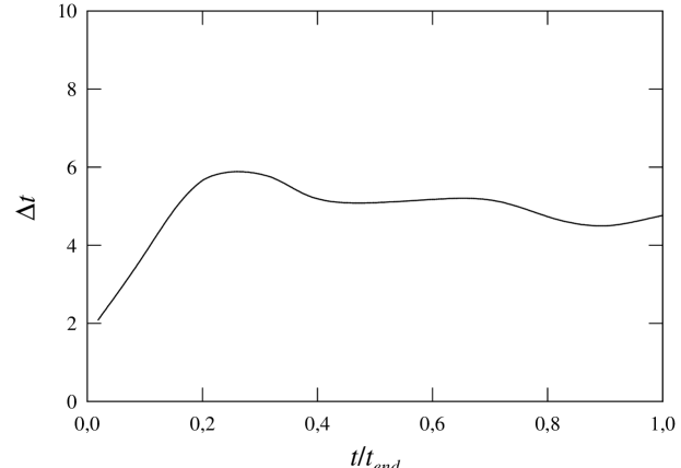
Figure 1: Ratio of the CPU time consumed by an algorithm where all particles are simultaneously advanced to that consumed when individual timesteps are considered.

Fig 1 shows, for a typical cosmological simulation, the ratio of the CPU time consumed by an algorithm with individual timesteps to that consumed when all particles are simultaneously advanced. We see that the use of individual timesteps typically reduces the CPU time per step in a factor of five. In a pentium IV 1.7GHz personal computer, the CPU time typically consumed by our code in a $2\times 64^{3}$ cosmological simulation without the ${\mathbf{\nabla}}h$ terms is: a) 25 seconds per step in simulations without radiative cooling (such as the Santa Barbara cluster test of §5.1), b) from 25 (at high redshifts) to 70 (at low redshifts) seconds per step in cosmological simulations with radiative cooling (such as those of §5.2). These CPU times are increased by about 150% when the ${\mathbf{\nabla}}h$ terms are taken into account.

4 Adiabatic Tests

DEVA has been applied to different problems with known analytical or numerical solutions. The aim of such simulations was not only to test our code, but also to analyze the effects of the ${\mathbf{\nabla}}h$ terms included in it.

4.1 The one-dimensional shock tube problem

The one-dimensional shock tube problem proposed by Sod (1978) has become a standard test of all transport and source terms (including artificial viscosities) of hydrodynamic algorithms. It considers a perfect gas distributed on the $x$-axis. A diaphragm at $x_{0}$ initially separates two regions which have different densities and pressures. All particles are initially at rest. At time $t=0$ the diaphragm is broken and both regions start to interact. Nonlinear waves are then generated at the discontinuity and propagate into each region: a shock wave which moves from the high to the small pressure region, while the associated rarefaction wave moves in the inverse sense. The analytical solution to this problem has been given by Hawley, Smarr, & Wilson (1984) and Rasio & Shapiro (1991). In our simulation, we have considered $N=4096$ gas particles initially distributed in the interval $0\leq x<1$ according to:

$$\rho=1\;\;P=1\;\;v=0\;\;\; (\mbox{for\hskip 4.30554pt}x<0.5)$$

$$\rho=0.25\;\;P=0.1795\;\;v=0\;\;\; (\mbox{for\hskip 4.30554pt}x\geq 0.5)$$

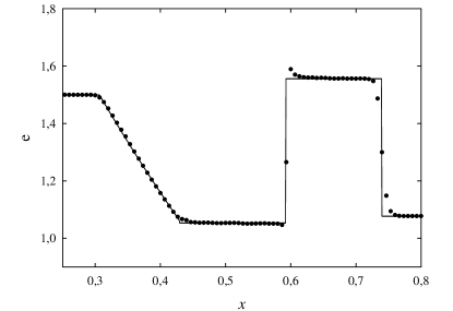
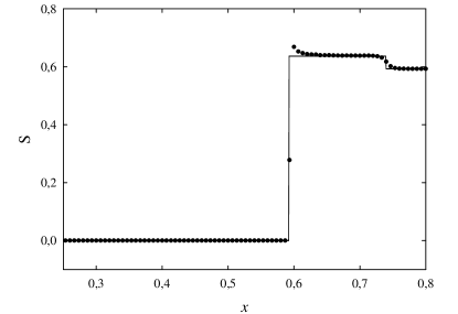
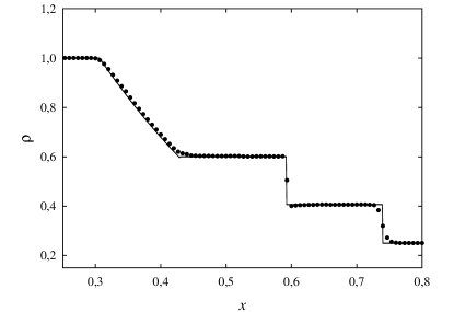
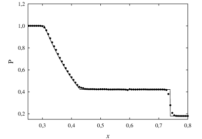
Figure 2: a) Thermal energy, b) entropy, c) density, and d) pressure profiles at $t=0.15$ in the one-dimensional shock tube problem. Points represent the DEVA results, and solid lines are the analytical solutions

Dissipational effects, other than those associated with the artificial viscosity (with $\alpha=\beta=1$ and $\eta^{2}=0.01$), were ignored, as well as gravitational interactions. Fig. 2 shows our results at $t=0.15$. We see from this figure that our results are in excellent agreement with the analytical solutions. The resulting profiles both in the shock wave (located at $x\simeq 0.75$) and in the contact discontinuity (located at $x\simeq 0.6$) are much less rounded than in previous SPH computations (see, e.g. Monaghan & Gingold, 1983; Hernquist & Katz, 1989; Rasio & Shapiro, 1991) as a result of having used a larger number of particles and, hence, a better resolution. We also note the almost complete suppression of post-shock oscillations in our results. These oscillations can be seen in the previous SPH simulations of this problem, especially in the velocity field, while no high-frequency vibrations are perceptible in our results. The weak blip observed in the pressure profile at the contact discontinuity ($x\simeq 0.6$) is normal in SPH codes. Such non-physical blip has been explained by Monaghan & Gingold (1983) as due to the fact that the smoothed estimate of pressure is computed by using discontinuous quantities. It is then inevitable that $P$ has some slight perturbation at the contact discontinuity, but it has a negligible effect on the motion. In this test, simulations including the ${\mathbf{\nabla}}h$ terms gave exactly the same results as those neglecting such terms.

4.2 Adiabatic collapse of a non-rotating gas sphere

A 3D-problem usually considered to test hydrodynamical codes is that concerning the adiabatic collapse of a non-rotating gas sphere. This problem has been studied from a finite-difference method by Thomas (1987), and from SPH simulations by Evrard (1988) and Hernquist & Katz (1989). In order to facilitate the comparison of our results to those obtained by these authors, we have taken their same initial conditions: a gas sphere of radius $R$ and total mass $M_{T}$, with density profile

$$\rho=\frac{M_{T}}{2\pi R^{2}}\frac{1}{r}\;.$$ (28)

All the $N=4096$ gas particles are initially at rest and have the same specific internal energy $u=0.05GM_{T}/R$. Units were taken so that $2G=M_{T}=2R=1$. Initially far from equilibrium, the system collapses converting most of its kinetic energy into heat. A slow expansion follows and, at late times, a core-halo structure develops with nearly isothermal inner regions and the outer regions cooling adiabatically. We show in Fig. 3 different system profiles at end of the simulation. The solid line represents the numerical solution obtained when the ${\mathbf{\nabla}}h$ terms have been included, the dashed line represents the numerical solution obtained when these terms have been neglected, and the points represent the numerical solution obtained by Hernquist & Katz (1989). We see that, although the solid and dashed lines are not exactly superposed, both solutions are coincident within the error bars.

4.3 Interpretation of the influence of the ${\mathbf{\nabla}}h$ terms

We can understand why the ${\mathbf{\nabla}}h$ terms have a negligible effect in the two standard tests reported in this section. The effect of the ${\mathbf{\nabla}}h$ terms on the thermal energy can be expressed by a time scale defined by

$$t_{S}=\langle t_{S}^{i}\rangle\;,$$ (29)

where $t_{S}^{i}$ is the ratio of the specific thermal energy $u_{i}$ of particle $i$ to the change in $u_{i}$ due to the ${\mathbf{\nabla}}h$ terms

$$t_{S}^{i}=\frac{u_{i}}{\dot{u}_{i}^{{\mathbf{\nabla}}h}}\;.$$ (30)

When the time elapsed, $t$, is longer than this time scale, the ${\mathbf{\nabla}}h$ terms will produce a non-negligible effect on the thermal energy. This condition can be expressed as

$$I=\int_{0}^{t}\frac{dt^{\prime}}{t_{S}(t^{\prime})}\geq 1\;,$$ (31)

where $I$ represents the area contained by the $1/t_{S}(t^{\prime})$ curve between $t^{\prime}=0$ and $t^{\prime}=t$.

When these timescales are computed for the non-adiabatic tests reported in this paper, one obtains $I=0.001$ (in the shock tube problem), and $I=0.85$ (in the collapse of a non-rotating gas sphere). The effect of the ${\mathbf{\nabla}}h$ terms are then expected to be small.

4.4 Quntifying the effects of the $\nabla h$ terms

Testing the effects of the $\nabla h$ terms on hydrodynamical evolution can be better worked out in isentropic processes. It is not easy, however, to get such kind of processes in simulations of gas evolution because gas easily develops shocks where dissipation must occur. A possibility is considering the adiabatic expansion of a gas sphere from a situation of equilibrium. Using expansion rather than collapse has the advantage that shell crossing decreases substantially, so that viscous force terms can be removed and the evolution is isentropic.

Such simulations as that shown in §4.2 lead at late times, $t\gtrsim 3$, to equilibrium spheres with density profiles as that displayed in Fig. 3. We use the adiabatic expansion of such spheres to test the effects of the ${\mathbf{\nabla}}h$ terms in DEVA. Initial conditions were generated by performing a simulation as that described in §4.2, using different numbers of particles. At $t=3$, we switched-off its viscous pressures (by setting $\alpha=\beta=0$) to ensure that the subsequent evolution conserves the total entropy. The self-gravity was also switched-off at $t=3$. In absence of gravitational interactions, this system expands fast and, at $t=3.3$, its central density has decreased by a factor of $\approx 25$. The evolution from $t=3$ to $t=3.3$ must conserve both the total energy and entropy.

Table 1 shows the results for this series of simulations. We see that, when the ${\mathbf{\nabla}}h$ correction terms are neglected, energy is conserved very accurately but there exists a considerable violation of the total entropy (about $5\%$ in the time interval we have considered). In the opposite case, when such correction terms are taken into account, both total energy and total entropy are conserved very accurately (about $0.02\%$). These results appear to be independent on the number of particles. We then conclude that the ${\mathbf{\nabla}}h$ correction terms cure entropy violation, allowing, at the same time, a very good energy conservation.

5 Self-Consistent Cosmological Simulations

The DEVA code is particularly well suited to numerically follow, in a cosmological context, the assembly from the field of primordial fluctuations of collapsed objects, such as galaxy clusters or galaxies. To illustrate DEVA performances in this situation, we briefly analyze some results of self-consistent simulations. Self-consistency means that initial conditions are set at high $z$ as a Montecarlo realization of the field of primordial fluctuations (i.e., perturbations, characterized by a spectrum, to a given cosmological model), and then they are left to evolve according with Newton’s laws and the hydrodynamical equations.

5.1 The Santa Barbara cluster test

The Santa Barbara cluster problem was proposed by Frenk et al. (1999) to compare the results obtained from different codes. The formation of a X-ray cluster in a Cold Dark Matter (CDM) universe has been simulated using most of the hydrodynamic codes available at that time, setting a standard of reference to test newly proposed hydrodynamic codes.

The initial conditions of this test correspond to a $3\sigma$ peak of the density field smoothed with a Gaussian filter of radius $r_{0}=10$ Mpc according to the algorithm of Hoffman & Ribak (1991). The perturbation was centered on a periodic cubic region of side $L=64$ Mpc. The cosmological scenario is a flat CDM universe with $H_{0}=50$ km s^-1 Mpc^-1 for the Hubble constant; $\sigma_{8}=0.9$ for the present-day linear rms mass fluctuation in spherical top hat spheres of radius 16 Mpc; and $\Omega_{b}=0.1$ for the baryon density (in units of the critical density). 64³ dark matter and 64³ baryon particles have been used with a softening length of 20 kpc.

To test the influence of the ${\mathbf{\nabla}}h$ terms, two different simulations were run with DEVA. In one of these simulations, the ${\mathbf{\nabla}}h$ terms have been considered (SBGH) while in the other they have been neglected (SBnoGH). In Figure 4, the density, temperature and entropy profiles of the cluster are plot. The stars represent the results obtained (Frenk et al., 1999) by Jenkins from a high-resolution SPH simulation using a parallel version of the Hydra code (Pearce & Couchman, 1997), while the circles represent the results obtained by Bryan & Norman from a high-resolution adaptive mesh refinement shock-capturing code, SAMR, (Bryan et al., 1995; Bryan & Norman, 1995). As previously remarked by Frenk et al. (1999), we see that the SPH and mesh results differ at the central region. This figure also shows the results obtained from our code both when the ${\mathbf{\nabla}}h$ terms are included (solid line) and neglected (dashed line). Error bars correspond to the standard deviation of the individual SPH data.

We see that, now, our results differ slightly depending on whether the ${\mathbf{\nabla}}h$ terms have been included or not (the slope of the density profile flattens more rapidly in SBGH than in SBnoGH; the temperature profile is flat in SBGH and decreases within 100 kpc in SBnoGH; the entropy profile is almost flat within 100 kpc in SBGH and decreases continuously in SBnoGH). Moreover, when the ${\mathbf{\nabla}}h$ terms are neglected, we obtain results that are similar to those of previous SPH simulations, and very close to Jenkins’ results, obtained with a much higher resolution. When these terms are taken into account, the results are intermediate between previous SPH and grid results. This suggests that, at least in part, the difference between the SPH and grid results could be due to the non-physical entropy introduced by SPH codes. This non-physical entropy is negative (Alimi et al., 2002) and, therefore, it produces objects with a smaller central temperature and a higher central density.

Particular attention deserves the comparison of DEVA results with those obtained from the entropy conserving SPH-Tree formulation by Springel & Hernquist (2002a), hereafter S-GADGET. In Figure 5 we give a comparison of the Santa Barbara cluster entropy profiles obtained in the SBGH run and S-GADGET, kindly provided by Y. Ascasibar and G. Yepes (Ascasibar, 2003). Both have been run with the same number of particles and gravitational resolution. We see that the agreement is very good within the error bars. So, both techniques compare very well in terms of entropy conservation.

The differences found between SBGH and SBnoGH simulations can be understood on the basis of the timescale for the ${\mathbf{\nabla}}h$ terms (section 4.3). The time integral of $1/t_{S}$ (see Eq. 29) for this test is now larger than unity ($I=1.2$).

5.2 Two Flat $\Lambda$CDM Cosmological Models

We now report on several self-consistent simulations run in the context of flat $\Lambda$CDM cosmological models with the aim of studying galaxy assembly (see Table 2 for a summary). We have considered two different $\Lambda$CDM models with parameters whose values are consistent with their recent determinations from observations: simulations $\Lambda$CDM1 ($\Lambda$CDM2) have $\Omega_{\Lambda}=0.65$ (0.7), $\Omega_{\rm baryon}=0.07$ (0.04), $\sigma_{8}=1.18$ (1.00) and $h=0.65$ (0.70) (Lahav, 2002; Netterfield et al., 2002; Spergel et al., 2003, and references therein). Both simulations share the same seed for the Montecarlo realization of the initial fluctuation field, so that each object formed in one simulation has its counterpart in the other simulation. In each case, we have used $64^{3}$ DM particles and $64^{3}$ gas particles, in a periodic box of 10 Mpc comoving side. The gravitational softening is $\epsilon_{\rm g}=2.3$ kpc, and the minimum allowed smoothing length, $h=\epsilon_{\rm g}/2$, as usual. For each cosmological model, two simulations have been run that are identical (they have exactly the same initial conditions and the same values of the cosmological parameters) except that in one case the ${\mathbf{\nabla}}h$ terms have been included (simulations $\Lambda$CDM1-H and $\Lambda$CDM2-H hereafter), while in the second case these terms have not been taken into account (simulations $\Lambda$CDM1-NoH and $\Lambda$CDM2-NoH hereafter, see Table 2). Note that in these simulations the cosmological volume is homogeneously sampled, in the sense that no resampling multimass technique has been used to study GLO assembly. This work can be considered as an extension of previous works in standard CDM models (Domínguez-Tenreiro, Tissera & Sáiz, 1998; Sáiz et al., 2001; Tissera, 2001; Tissera et al., 2002), where cosmological simulations had been run with a different code based on a different numerical approach with fixed integration timesteps and particle masses (Tissera, Lambas & Abadi, 1997). Relative to these previous works, DEVA opens the possibility of considering the effects of the ${\mathbf{\nabla}}h$ terms at scales of galaxies in self-consistent simulations. Moreover, the simulations we report here represent an improvement of the baryonic mass resolution by factors of $\simeq 10$ in the number of baryonic particles sampling a GLO of a given total mass. Also, the time resolution allowed by the multistep technique has been improved by a factor of $\simeq 30$ in the denser areas of the box.

Cooling has been implemented as described in $\S$ 3.4, where the cooling curve is that from Tucker (1975) and Bond et al. (1984) for an optically thin primordial mixture of H and He ($X=0.76$, $Y=0.24$) in collisional equilibrium and in absence of any significant background radiation field.

Concerning star formation, in this work we report on direct results (i.e., no spectrophotometric) obtained with the simplest implementation of star formation in the code: through a parameterization, similar to those used by Katz (1992) and Tissera, Lambas & Abadi (1997), see Alimi et al. (2002) for details, based on the Jeans criterion for a collapsing region. Gas particles are turned into stars according with an inefficient Schmidt-law-like transformation rule (see Kennicutt, 1998; Silk, 2001),

$$\frac{d\rho_{g}}{dt}=-\frac{d\rho_{\ast}}{dt}=-\frac{c_{\ast}\rho_{g}}{t_{g}}\;,$$ (32)

where $c_{\ast}$ is a dimensionless star-formation efficiency parameter, and $t_{g}$ is a characteristic time-scale chosen to be equal to the maximum of the local gas-dynamical time $t_{dyn}=(4\pi G\rho_{g})^{-1/2}$, and the local cooling time, $t_{cool}=u_{i}/\dot{u}_{i}$. Equation (32) implies that the probability $p$ that a gas particle forms stars in a time $\Delta t$ is

$$p=1-e^{-c_{\ast}\Delta t/t_{g}}\;.$$ (33)

As usual, we compute $p$ at each time step for all eligible gas particles and draw random numbers to decide which particles actually form stars.

Stellar feedback processes have not been explicitly considered, but a tuning of the efficiency parameters can mimic these feedback effects. Galaxy-like objects of different morphologies appear in the simulation: disk-like objects (DLOs), early-type-like objects (ETLOs) and irregular objects. DLOs contain gas in an extended disk, and most stars in a massive compact central concentration. In simulations with lower $\epsilon_{\rm g}$ values (not reported here), stars form also in the disks, along arms. ETLOs are very poor in gas and their stellar component have relaxed regular ellipsoidal shapes. Irregulars have not defined shapes, and, in most cases, they are the product of a recent merger or interaction event. We note that GLOs formed in $\Lambda$CDM2-NoH and $\Lambda$CDM2-H tend to be of later type than their $\Lambda$CDM1-NoH or $\Lambda$CDM1-H counterparts, because of the lower values the parameters $\Omega_{\rm baryon}$ and $\sigma_{8}$ take in $\Lambda$CDM2 simulations (Domínguez-Tenreiro et al., 2003). First analyses of GLO formation and evolution in simulations run with the DEVA code are reported in Sáiz et al. (2002a, b); more details will be given elsewhere (Sáiz el al. 2003, in preparation). Here we focus on different aspects related with DEVA performances.

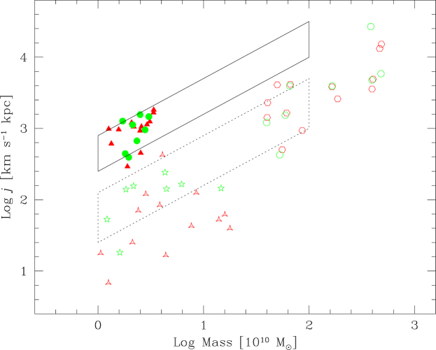
Figure 6: Specific total angular momentum versus mass for galaxy-like objects formed in $\Lambda$CDM2-NoH (triangles) and $\Lambda$CDM2-H (pentagons) with $V_{2.2}\geq 150$ km s^-1 at $z=0$. Open symbols: dark matter halos; filled symbols: the inner 83 per cent of the disc gas mass; starred symbols: central stellar component (see text). The solid (dashed) box encloses the region of the diagram corresponding to observed spirals (ellipticals)

One important issue related to disc formation in hydrodynamical simulations is specific angular momentum conservation at kpc scales (Sommer-Larsen & Dolgov, 2001; Steinmetz & Navarro, 1999; Domínguez-Tenreiro, Tissera & Sáiz, 1998; Sáiz et al., 2001). In Fig. 6, the specific total angular momentum at $z=0$ is represented versus mass for DLOs identified in $\Lambda$CDM2-NoH and $\Lambda$CDM2-H with $V_{\rm cir}(2.2R_{\rm d})\geq$ 150 km s^-1 ($R_{\rm d}$ is the disc scalelength, see Sáiz et al., 2001). The specific total angular momentum is plot for dark haloes, $j_{\rm dm}$ (open symbols), for the inner 83 per cent of the disc gas mass (i.e., the mass fraction enclosed by $R_{\rm opt}\equiv 3.2R_{\rm d}$ in a purely exponential disc), $j_{\rm g}$ (filled symbols), and for the stellar component of the DLOs in our simulations, $j_{\rm s}$ (starred symbols). We see that, except for the three more massive objects, $j_{\rm g}$ is of the same order as $j_{\rm dm}$, so that these gas particles have collapsed conserving, on average, their angular momentum. Moreover, DLOs formed in our simulations are inside the box defined by observed spiral discs in this plot (Fall, 1983). In contrast, $j_{\rm s}$ is much smaller than either $j_{\rm dm}$ or $j_{\rm g}$, meaning that the stellar component in the central parts has formed out of gas that had lost an important amount of its angular momentum in catastrophic events or that had never acquired it. We note that this result is similar to those obtained in simulations run with the code by Tissera, Lambas & Abadi (1997), even if the codes are different, as explained above, and that the global cosmological models are also different.

The smoothed estimate of the local gas density given by Eq. (2) and the ensuing formulation of SPH equations, symmetrized to ensure the reciprocity principle, has made possible $j_{\rm g}$ conservation in an axisymmetric potential. This is a delicate crucial point in SPH codes. As stated in $\S$2.2, its accurate implementation requires that the individual smoothing lengths must be completely updated at the beginning of each integration step, what increases the CPU time requirements. This complication cannot be avoided, however, when an accurate $j_{\rm g}$ conservation is a key point in the physical processes under study. A different approach to saving CPU time is then necessary. Using different timesteps for each particle, useless computations for particles that do not require high time resolution are avoided. This saves considerable amounts of CPU time. Multistepping has allowed us to run these simulations, that have a considerable dynamical range, in a modest computing machine (a pentium IV 1.7GHz personal computer, see above).

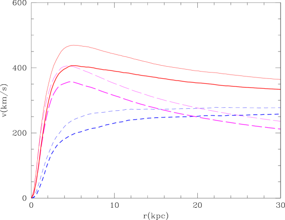
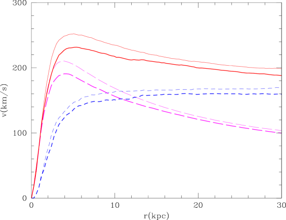
Figure 7: Circular velocity curves for two ETLOs (upper panel) and two DLOs (lower panel). ETLOs have formed in $\Lambda$CDM1-H (thick lines) and $\Lambda$CDM1-NoH (thin lines); DLOs have formed in $\Lambda$CDM2-H (thick lines) and $\Lambda$CDM2-NoH (thin lines). Short-dashed and long-dashed lines stand for the dark matter and the baryonic (both stellar and luminous) contributions to the circular velocity (solid line)

Let us now turn to the effects of the ${\mathbf{\nabla}}h$ terms at kpc scales. As stated in $\S$4.3, their general effect is to correct the spurious negative entropy introduced in their absence by SPH codes, mainly at the central regions of collapsed objects. As a consequence, when the ${\mathbf{\nabla}}h$ terms are taken into account, dissipation by the gaseous component of a given GLO increases, so that they are more disordered or dynamically hotter at their central regions. Equilibrium is then attained with lower central baryon concentrations or densities, decreasing the amount of gas infall. But this is not the unique effect of ${\mathbf{\nabla}}h$ terms on mass distribution. It is a well known effect that dark matter is pulled in by baryons as they lose their energy and fall onto these central volumes of collapsed configurations (Dalcanton, Spergel & Summers, 1997; Tissera & Domínguez-Tenreiro, 1998). Decreasing the amount of gas infall translates, as a consequence, into a decreasing of the amount of dark matter at the GLO centers. As an illustration of this effect on both the gaseous and dark components, in Figure 7 (upper panel) we show the circular velocity curves for the most massive ETLO formed in $\Lambda$CDM1-H (thick lines) and its counterpart formed in $\Lambda$CDM1-NoH (thin lines). In the lower panel, the corresponding circular velocity curves are represented for a DLO formed in $\Lambda$CDM2-H (thick lines) and its counterpart in $\Lambda$CDM2-NoH (thin lines). In these Figures, $r$ is the radial distance to the GLO center of mass, solid lines are the circular velocities, $V^{2}_{\rm cir}(r)=V^{2}_{\rm dm}(r)+V^{2}_{\rm bar}(r)$, short-dashed lines and long-dashed lines stand for the dark matter (dm) and the baryonic (bar, both stellar and luminous) contributions, respectively, given by:

$$V^{2}_{\rm i}(r)=\frac{GM_{\rm i}(<r)r^{2}}{(r^{2}+\epsilon_{\rm g}^{2})^{3/2}}\;,$$ (34)

with $i$ = bar and dm. As can be clearly seen in these Figures, the central distributions of both, dark matter and baryons, are different and in any case the concentrations are lower when the ${\mathbf{\nabla}}h$ terms are included. These central concentrations are often quantitatively estimated in literature through the $V_{\rm cir}^{\rm peak}$ parameter (the maximum or peak circular velocity, see Courteau, 1997; Sáiz et al., 2001). GLOs in $\Lambda$CDM1-H or $\Lambda$CDM2-H have lower $V_{\rm cir}^{\rm peak}$ values than their $\Lambda$CDM1-NoH and $\Lambda$CDM2-NoH counterparts, respectively. This can be seen in Figure 7 for an ETLO and a DLO, but the behavior is general for any GLO. Other useful parameter to quantitatively characterize circular velocity curves is the logarithmic slope (LS), observationally defined for disc rotation curves as the slope of the straight line that fits $V_{\rm cir}(r)$ in log-log scale from $R_{2.2}=2.2R_{\rm d}$ up to the last measured point in the rotation curve (Sáiz et al., 2001, and references therein; $R_{\rm d}$ is the disk scalelength). LSs are a measure of the GLO halo compactness at the scales of 10 - 30 kpcs. As illustrated in Figure 7 for an ETLO and a GLO, a tendency for GLOs to be less compact also at these scales when the ${\mathbf{\nabla}}h$ terms are taken into account has been found in the simulations.

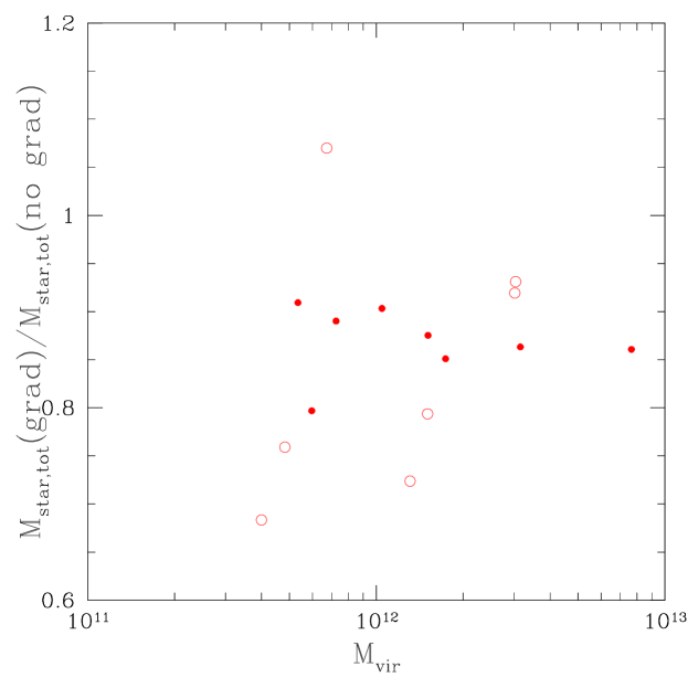
Figure 8: The total stellar mass inside the virial radii of ETLOs formed in $\Lambda$CDM1-H (filled symbols) and $\Lambda$CDM2-H (open symbols) in units of their $\Lambda$CDM1-NoH and $\Lambda$CDM2-NoH counterparts (where the ${\mathbf{\nabla}}h$ terms have not been taken into account), versus their virial masses

A second effect of the ${\mathbf{\nabla}}h$ terms is related to the amounts of stars formed in a given GLO at its formation and all along its evolution until $z=0$. In these simulations, many stars form at the shock fronts, where gas is compressed to very high densities. Softer shocks mean less star formation with the same efficiency parameters. To illustrate this effect, in Figure 8 the ratios of the total stellar masses for the 8 (7) more massive ETLOs produced in $\Lambda$CDM1-H ($\Lambda$CDM2-H) over the total stellar masses of their $\Lambda$CDM1-NoH ($\Lambda$CDM2-NoH) counterparts, are plot versus their total virial masses, $M_{\rm vir}$. We see that, except in one case, these ratios are smaller than the unity, as expected.

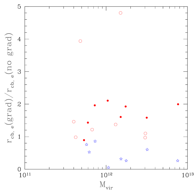
Figure 9: The 3D cold baryon effective radii of ETLOs formed in $\Lambda$CDM1-H (filled circles) and $\Lambda$CDM2-H (open circles) in units of their $\Lambda$CDM1-NoH and $\Lambda$CDM2-NoH counterparts (where the ${\mathbf{\nabla}}h$ terms have not been taken into account), versus their virial masses. Starred symbols stand for 3D cold baryon effective radii of ETLOs formed in $\Lambda$CDM1-MCool in units of their $\Lambda$CDM1-NoH counterparts (see Table and text)

Concerning sizes, for ETLOs we define the intrinsic or 3D cold baryon effective radius, $r_{\rm cb,e}$, as the radius of the sphere enclosing half the total ETLO mass in cold baryons (i.e., cold gas or stars), ${M}_{\rm cb,tot}$. This is a measure of the ETLO size at scales of the baryonic objects. In Figure 9 we plot $r_{\rm cb,e}$ for the $\Lambda$CDM1-H ($\Lambda$CDM2-H) ETLOs in units of those of their $\Lambda$CDM1-NoH ($\Lambda$CDM2-NoH) counterparts. As expected, $\Lambda$CDM1-H ($\Lambda$CDM2-H) ETLOS have larger baryonic sizes than their $\Lambda$CDM1-NoH ($\Lambda$CDM2-NoH) counterparts, except for one case.

Finally, shocks heat the gas, producing an extended diffuse hot component. The effect of the ${\mathbf{\nabla}}h$ terms in this case is to lower the temperature of this diffuse gaseous halo component of GLOs relative to the case when these terms are not considered. Histograms for the temperature distribution of the gaseous component of two of the most massive GLOs in $\Lambda$CDM1-H (thick lines) and in $\Lambda$CDM1-NoH (thin lines) are shown in Figure 10. To draw these histograms, all the gas particles within a sphere of radius $r_{\rm lim}$, centered at the GLO center of mass, have been considered ($r_{\rm lim}$ is the radius where the curve of integrated plasma emission luminosity reaches its asymptotic value). As illustrated in the histograms for these two GLOs, the temperature distributions of the gaseous component for $\Lambda$CDM1-H and $\Lambda$CDM1-NoH objects do not differ substantially. In both cases, the gas is close to biphasic, but $\Lambda$CDM1-H objects are slightly colder within $r_{\rm lim}$ than $\Lambda$CDM1-NoH objects. They are also slightly more extended at $r_{\rm lim}$ scales, with the small excess of colder particles placed at the outskirts of the gaseous configurations.

The differences found between $\Lambda$CDM1-H and $\Lambda$CDM1-NoH or between $\Lambda$CDM2-H and $\Lambda$CDM2-NoH simulations can be understood on the basis of the timescale for the ${\mathbf{\nabla}}h$ terms (section 4.3). The time integral of $1/t_{S}$ (see Eq. 29) is now much larger than unity ($I\simeq 80$), indicating that the ${\mathbf{\nabla}}h$ terms cannot be neglected in this kind of simulations.

As remarked in $\S$3.2, cooling implementation in multistep codes has to be handled with caution: cooling processes need to be updated at each timestep for all particles. Otherwise, gas particles involved in shocks suffer from a spurious cooling and non-physical cores of high density appear, giving rise to extremely compact objects. As an example, in Figure 9 we plot the 3D cold baryon half-mass radii for a variant of $\Lambda$CDM1-NoH, termed $\Lambda$CDM1-MCool (see Table 2 for details), where only active particles at each timestep have been allowed to cool. In Figure 9 (starred symbols) we see that now the effective radii for the most massive objects are significantly smaller than in $\Lambda$CDM1-NoH; the difference becomes less important as the mass of the objects decreases and, as a consequence, the fraction of their constituent particles involved in shocks also decreases. Note that, as the comparison of filled points and starred symbols in Figure 9 shows, the combined effects of entropy violation and spurious cooling can produce unphysically very small objects, a factor of ten smaller, in some cases, than the values found when these effects are circumvented (i.e., the $\Lambda$CDM1-H simulation).

6 Summary, Discussion and Conclusions

We present DEVA, a multistep AP3M-like-SPH code designed to study galaxy formation and evolution in connection with the global cosmological model, that uses a formulation of SPH equations ensuring both energy and entropy conservation.

Multistepping is introduced to save CPU time. In self-consistent cosmological simulations multiple time scales appear, due to their large dynamical ranges. To avoid that particles in denser zones slow down the simulation, and, at the same time, to get a properly accurate integration algorithm, it is then advantageous to use individual time steps. A comparison of the CPU time used in a self-consistent cosmological simulation when it is run with a global timestep or with a multistep scheme indicates that in the second case results at an equivalent level of accuracy are produced $\sim$5 times faster.

When a multistep scheme is adopted, a delicate issue in the study of galaxy assembly in a cosmological context is the cooling implementation. In DEVA, as no cooling timescale is taken into consideration to fix the individual timestep for each particle, cooling must be calculated in a non-multistep way. Otherwise, particles involved in strong shocks would spuriously cool and form dense objects characterized by unphysically small baryon half-mass radii.

On writting DEVA, particular attention was paid that conservation laws of physics (energy, entropy, momentum) are correctly implemented in the code, so that they hold at scales and under physical conditions relevant for galaxy assembly in a cosmological context. The usual formulations of SPH equations focus on energy conservation and they violate, by construction, entropy conservation. As a consequence, a negative entropy is numerically produced in shocks that might (or might not) spuriously pollute the results, depending on the problem one studies. Different authors have addressed the issue of entropy violation in SPH codes (Nelson & Papaloizou, 1993, 1994; Hernquist, 1993; Springel & Hernquist, 2002a) and have given different alternative formulations of its equations. We have implemented a formulation that considers explicitly the effects of the ${\mathbf{\nabla}}h$ terms in SPH equations (Nelson & Papaloizou, 1994). By taking advantage of the structure of the AP3M algorithm in the neighbor search, the implementation of ${\mathbf{\nabla}}h$ terms in the code is simple and noiseless.

To test the relevance of entropy violation at shock locations under different physical conditions, we have studied problems and run simulations (namely, the adiabatic Santa Barbara cluster formation test, Frenk et al. (1999), and fully self-consistent cosmological simulations to study galaxy formation including cooling an star formation) using identical initial conditions and two different versions of DEVA, one that takes into account the ${\mathbf{\nabla}}h$ terms in SPH equations and one that does not take them into account. We show that entropy violation has consequences on the thermodynamical properties of the very central regions of the Santa Barbara cluster and on the structure at kpc scales of galaxy-like objects (GLOs) formed in simulations, but it does not have any appreciable consequence on the standard non-cosmological tests of hydrodynamical codes. To understand the origins of these different behaviors, a criterion is introduced that allows to elucidate when entropy violation is expected to have appreciable consequences on the results. In standard tests, only moderate shocks and time scales are involved.

As a consequence of the non-physical negative entropy numerically produced when the ${\mathbf{\nabla}}h$ terms are neglected, both GLOs and the cluster present more concentrated baryon density profiles (either star or gas). Concerning the Santa Barbara cluster test, when the ${\mathbf{\nabla}}h$ terms are not included, we get results that are similar to those of previous SPH simulations that focus on energy conservation. However, when these terms are considered, the results are intermediate between those SPH and grid results. For example, the temperature profile is decreasing within about 100 kpc of the cluster center when the simulation is run with standard SPH codes (including DEVA without ${\mathbf{\nabla}}h$ terms), it increases when it is run with grid codes and it is flat when DEVA + ${\mathbf{\nabla}}h$ is used. We would like to note that the accuracy figure of entropy conservation obtained with DEVA + ${\mathbf{\nabla}}h$ and the entropy-conserving SPH-Tree code by Springel & Hernquist (S-GADGET, 2002a) compare quite satisfactorily, as indicated by the good agreement between the Santa Barbara cluster entropy profiles obtained with both codes.

In cosmological simulations, negative entropy causes galaxy-like objects (GLOs) to be dynamically less hot and gas infall onto their central regions is artificially increased, causing, also, an increase of the amount of dark matter at the GLO centers. These results qualitatively agree with those obtained with S-GADGET by Springel & Hernquist (2002a) in their simulation of a $\Lambda$CDM cosmological model. No quantitative comparisons are possible by the moment, because a standard of comparison for self-consistent cosmological simulations is unfortunately not available.

An important result of this work is that the combined effects of entropy violation and multi-step cooling implementation in cosmological simulations can be particularly dramatic concerning the concentration of mass distribution in the galaxy-like objects they produce. For example, their baryon half-mass radii can be up to a factor of ten smaller than half-mass radii of GLOs produced in entropy-conserving non-multistep runs with DEVA.

Concerning momentum conservation, we have used a formulation of SPH equations that is consistent with the smoothed estimate of the local gas density (Eqs (1) and (3)). Equations are symmetrized to ensure that the reciprocity principle holds (that is, if at a given time the $j$th particle belongs to the neighbor list of the $i$th particle, then it is mandatory that, at this same time, the $i$th particle belongs to the neighbor list of the $j$th particle), so that momentum and angular momentum are conserved. The implementation of this principle in a SPH code increases considerably the CPU time per integration step, because a double loop on gas particles is necessary to evaluate smoothing lengths. To test angular momentum conservation, we have measured the specific angular momentum of discs formed in self-consistent simulations. It has been found that conservation is good enough to obtain simulated discs with observational counterparts, without any need of previous heating, as already Sáiz et al. (2001) have shown (see also Governato et al., 2002).

The use of a very high number of particles could ensure angular momentum conservation in SPH-tree codes (Governato et al., 2002). In this paper it has been shown that codes paying a particular attention to the implementation of conservation laws of physics at the scales of interest can attain a good level of accuracy in conservation laws with more limited resources.

TABLE 1

Entropy and Energy Conservation

Run	${\mathbf{\nabla}}h$ terms	$N$	$\Delta E$	$\Delta S$
HTest1	Excluded	1024	0.01%	5.6%
HTest2	Included	1024	0.02%	0.02%
HTest3	Excluded	2048	0.01%	5.2%
HTest4	Included	2048	0.01%	0.01%
HTest5	Excluded	4096	0.02%	5.5%
HTest6	Included	4096	0.01%	0.02%

TABLE 2

Summary of $\Lambda$CDM Simulations

Run	$\Omega_{\Lambda}$	$\Omega_{B}$	$\sigma_{8}$	$h$	${\mathbf{\nabla}}h$ terms	Cooling
$\Lambda$CDM1-H	0.65	0.07	1.18	0.65	Yes	Non-multistep
$\Lambda$CDM1-NoH	0.65	0.07	1.18	0.65	No	Non-multistep
$\Lambda$CDM1-MCool	0.65	0.07	1.18	0.65	No	Multistep
$\Lambda$CDM2-H	0.70	0.04	1.00	0.70	Yes	Non-multistep
$\Lambda$CDM2-NoH	0.70	0.04	1.00	0.70	No	Non-multistep

   

   

Figure 3: Final gas density, thermal energy, pressure and radial velocity profiles for the adiabatic collapse of a non-rotating gas sphere. Stars: Hernquist & Katz (1989) results. Solid (dashed) line: DEVA results when the ${\mathbf{\nabla}}h$ terms are (are not) taken into account, with their corresponding errors (see text)

Figure 4: Density, temperature and entropy profiles in the Santa Barbara cluster test. The stars represent the SPH results obtained by Jenkins, while circles represent the results obtained by Bryan & Norman from an adaptive mesh refinement code. The lines correspond to the results obtained from DEVA when the ${\mathbf{\nabla}}h$ terms are taken into account (solid line) and when these terms are neglected (dashed line)

Figure 5: Comparison of the Santa Barbara entropy profiles obtained from the entropy conserving versions of DEVA (solid line) and GADGET (symbols)

Figure 10: Histograms for the temperature distribution of the gas particles sampling two of the most massive ETLOs formed in $\Lambda$CDM1-H (thick lines) and for their counterparts formed in $\Lambda$CDM1-NoH (thin lines)

References

- Alimi et al. (2002) Alimi J.-M., Serna A., Pastor C. & Bernabeu G. 2002, J. Comput. Phys. (in press)
- Ascasibar (2003) Ascasibar, Y. 2003, PhD Thesis, Universidad Autónoma de Madrid
- Avila-Reese & Vázquez-Semadeni (2001) Avila-Reese, V., & Vázquez-Semadeni, E. 2001, ApJ, 553, 645
- Barnes (1989) Barnes, J.E. 1989, Nature, 338, 123
- Barnes (1992) Barnes, J.E., 1992, ApJ, 393, 484
- Barnes & Hernquist (1991) Barnes, J. E. & Hernquist, L. E. 1991, ApJ, 370, L65
- Barnes & Hernquist (1992) Barnes, J. E. & Hernquist, L. 1992, ARA&A, 30, 705
- Barnes & Hut (1986) Barnes J., & Hut P. 1986, Nature324, 446
- Benz & Hills (1987) Benz, W. & Hills, J. G. 1987, ApJ, 323, 614
- Bond et al. (1984) Bond, J. R., Centrella, J., Szalay, A. S., & Wilson, J. R. 1984, MNRAS, 210, 515
- Borgani et al. (2002) Borgani, S., Governato, F., Wadsley, J., Menci, N., Tozzi, P., Quinn, T., Stadel, J., & Lake, G. 2002, MNRAS, 336, 409
- Bryan et al. (1995) Bryan, G.L., Norman, M.L., Stone, J.M., Cen, R., & Ostriker, J.P. 1995, Comput. Phys. Comm., 89, 149
- Bryan & Norman (1995) Bryan, G.L., & Norman, M.L. 1995, BAAS, 187, 9504
- Couchman (1991) Couchman, H. M. P. 1991, ApJ, 368, L23
- Couchman, Thomas, & Pearce (1995) Couchman, H.M.P., Thomas, & Pierce, F.R., 1995, ApJ, 452, 797
- Courteau (1997) Courteau, S. 1997, AJ, 114, 2402
- Dalcanton, Spergel & Summers (1997) Dalcanton, J. J., Spergel, D. N., & Summers, F. J. 1997, ApJ, 482, 659
- Davé, Dubinski, & Hernquist (1997) Dave, R., Dubinski, J., & Hernquist, L. 1997, New Astronomy, 2, 277
- Domínguez-Tenreiro et al. (2003) Domínguez-Tenreiro, R., Serna, A., Sáiz, A., & Sierra-González de Buitrago, M. M. 2003, Ap&SS, in press
- Domínguez-Tenreiro, Tissera & Sáiz (1998) Domínguez-Tenreiro, R., Tissera, P. B., & Sáiz, A. 1998, ApJ, 508, L123
- Elmegreen (2003) Elmegreen, B. 2003, Ap&SS, in press
- Evrard (1988) Evrard, A. E. 1988, MNRAS, 235, 911
- Fall (1983) Fall, S.M. 1983, in Athanassoula E., ed, IUA Symp. 100, Internal Kinematics and Dynamics of Galaxies. Reidel, Dordrecht, p. 391
- Frenk et al. (1999) Frenk, C. S. et al. 1999, ApJ, 525, 554
- Gingold & Monaghan (1977) Gingold R. A. & Monaghan J. J. 1977, MNRAS, 181, 375
- Gingold & Monaghan (1982) Gingold R. A. & Monaghan J. J. 1982, J. Comput. Phys. 46, 429
- Godunov (1959) Godunov, S. K. 1959, Matematicheskii Sbornik, 47, 271
- Governato et al. (2002) Governato, F., Mayer, L., Wadsley, J., Gardner, J.P., Willman, B., Hayashi, E., Quinn, T., Stadel, J., & Lake, G. 2002, astro-ph/0207044 preprint
- Hawley, Smarr, & Wilson (1984) Hawley, J. F., Smarr, L. L., & Wilson, J. R. 1984, ApJ, 277, 296
- Hernquist (1993) Hernquist, L. 1993, ApJ, 404, 717
- Hernquist & Katz (1989) Hernquist, L. & Katz, N. 1989, ApJS, 70, 419
- Hoffman & Ribak (1991) Hoffman, Y. & Ribak, E. 1991, ApJ, 380, L5
- Kang et al. (1994) Kang, H., Ostriker, J. P., Cen, R., Ryu, D., Hernquist, L., Evrard, A. E., Bryan, G. L., & Norman, M. L. 1994, ApJ, 430, 83
- Katz (1992) Katz N. 1992, ApJ391, 502
- Katz, Weinberg, & Hernquist (1996) Katz, N., Weinberg, D. H., & Hernquist, L. 1996, ApJS, 105, 19
- Kennicutt (1998) Kennicutt, R. 1998, ApJ, 498, 541
- Klein et al. (1998) Klein, R.I., Fisher, R.T., McKee, C.F. & Truelove, J.K. 1998, in Proceedings of the International Conference of Numerical Astrophysics, ed. S ..M. Miyama et al. (Boston: Kluwer Academic), p. 131
- Knebe, Green & Binney (2001) Knebe, A., Green, A., & Binney, J. 2001, MNRAS, 325, 845
- Knebe et al. (2000) Knebe, A., Kravtsov, A. V., Gottlöber, S., & Klypin, A. A. 2000, MNRAS, 317, 630
- Kravtsov, Klypin & Khokhlov (1997) Kravtsov, A. V., Klypin, A. A., & Khokhlov, A. M. 1997, ApJS, 111, 73
- Kritsuk & Norman (2002) Kritsuk, A. G. & Norman, M. L. 2002, ApJ, 569, L127
- Lahav (2002) Lahav, O. 2002, in Proceedings of the XXXVIIth Rencontres de Moriond on The Cosmological Model, astro-ph/0208297 preprint
- Lahav et al. (2002) Lahav, O., Bridle, L., Percival, W.J., et al. 2002, astro-ph/0112162 preprint
- Lucy (1977) Lucy, L. B. 1977, AJ, 82, 1013
- Mihos & Hernquist (1994) Mihos, J. C. & Hernquist, L. 1994, ApJ, 425, L13
- Mihos & Hernquist (1996) Mihos, J. C. & Hernquist, L. 1996, ApJ, 464, 641
- Monaghan (1992) Monaghan, J. J. 1992, ARA&A, 30, 543
- Monaghan & Gingold (1983) Monaghan J. J. & Gingold R. A. 1983, J. Comput. Phys., 52, 374
- Monaghan & Lattanzio (1985) Monaghan, J. J. & Lattanzio, J. C. 1985, A&A, 149, 135
- Navarro & White (1993) Navarro, J. F. & White, S. D. M. 1993, MNRAS, 265, 271
- Nelson & Papaloizou (1993) Nelson, R. P. & Papaloizou, J. C. B. 1993, MNRAS, 265, 905
- Nelson & Papaloizou (1994) Nelson, R. P. & Papaloizou, J. C. B. 1994, MNRAS, 270, 1
- Netterfield et al. (2002) Netterfield, C. B. et al. 2002, ApJ, 571, 604
- Norman & Bryan (1998) Norman, M. L. & Bryan, G.L. 1998, in Proceedings of the International Conference of Numerical astrophysics, ed. S.M. Miyama et al. (Boston: Kluwer Academic), p. 19
- Padoan et al. (2003) Padoan, P., Jimenez, R., Nordlund, A., & Boldyrev, S. 2003, astro-ph/0301026 preprint
- Padoan et al. (1999) Padoan, P., Juvela, M., Goodman, A. & Nordlund, A. 2001, ApJ, 553, 227
- Pearce & Couchman (1997) Pearce, F. R. & Couchman, H. M. P. 1997, New Astronomy, 2, 411
- Rasio & Shapiro (1991) Rasio, F. A. & Shapiro, S. L. 1991, ApJ, 377, 559
- Sáiz et al. (2002a) Sáiz A., Domínguez-Tenreiro R., & Serna, A. 2002, Ap&SS, 281, 309
- Sáiz et al. (2002b) Sáiz A., Domínguez-Tenreiro R., & Serna, A. 2003, Ap&SS, in press
- Sáiz et al. (2001) Sáiz, A., Domínguez-Tenreiro, R., Tissera, P. B., & Courteau, S. 2001, MNRAS, 325, 119
- Serna, Alimi, & Chièze (1996) Serna A., Alimi J.-M., & Chièze J.-P. 1996, ApJ, 461, 884
- Silk (2001) Silk, J. 2001, MNRAS, 324, 313
- Sod (1978) Sod, G. A. 1978, J. Comput. Phys., 27, 1
- Sommer-Larsen & Dolgov (2001) Sommer-Larsen J., & Dolgov A. 2001, ApJ, 551, 608
- Spergel et al. (2003) Spergel D. N. et al. 2003, astro-ph/0302209 preprint
- Springel & Hernquist (2002a) Springel, V. & Hernquist, L. 2002, MNRAS, 333, 649
- Springel & Hernquist (2002b) Springel, V. & Hernquist, L. 2002b, astro-ph/0206393 preprint
- Springel, Yoshida & White (2001) Springel, V., Yoshida, N. & White, S. 2001, New Astronomy, 6, 79
- Steinmetz (1996) Steinmetz, M. 1996, MNRAS, 278, 1005
- Steinmetz & Navarro (1999) Steinmetz, M. & Navarro, J. 1999, ApJ, 513, 555
- Teyssier (2002) Teyssier, R. 2002, A & A, in press
- Thacker & Couchman (2000) Thacker, R. J. & Couchman, H. M. P. 2000, ApJ, 545, 728
- Thomas (1987) Thomas P. A. 1987, Ph.D. thesis, Cambridge Univ.
- Thomas, & Couchman (1992) Thomas P. A. & Couchman H. M. P. 1992, MNRAS, 257, 11
- Tissera, Lambas & Abadi (1997) Tissera P. B., Lambas D. G., & Abadi M. G., 1997, MNRAS, 286, 384
- Tissera & Domínguez-Tenreiro (1998) Tissera P. B., & Domínguez-Tenreiro, R. 1998, MNRAS, 297, 177
- Tissera (2001) Tissera P. B. 2001, ApJ, 540, 384
- Tissera et al. (2002) Tissera, P.B., Domínguez-Tenreiro, R., Scannapieco, C., & Sáiz, A. 2002, MNRAS, 333, 327
- Tucker (1975) Tucker W. H. 1975, Radiation Precesses in Astrophysics (New York, Wiley)
- Vázquez-Semadeni et al. (2000) Vázquez-Semadeni, E., Ostriker, E. C., Passot, T., Gammie, C. F., & Stone, J. M. 2000, Protostars & Planets IV, ed. V. Mannings et al. (Tucson: Univ. of Arizona Press), in press
- Vedel, Hellsten & Sommer-Larsen (1999) Vedel, H., Hellsten, U., & Sommer-Larsen, J. 1999, MNRAS, 271, 743
- Verheijen, Bershady & Andersen (2002) Verheijen, M., Bershady, M., & Andersen D. 2002, Mass Galaxies at Low and High Redshift (ESO Workshop, Venice) pp. 24-26
- Wada & Norman (2001) Wada, K. & Norman, C. A. 2001, ApJ, 547, 172
- Yepes el al. (1997) Yepes, G., Kates, R., Khokhlov, A., & Klypin, A. 1997, MNRAS, 284, 235