1 Introduction

Experimental evidence for the existence of a cosmological constant has grown dramatically over recent years. It now seems likely that the cosmological constant, or some form of ‘dark energy’, is responsible for around 70% of the total energy density of the universe [1]. There are two attitudes one can take towards the dark energy. One is that it is a relic from symmetry breaking in a more complete theory, and as such has a field-theoretic origin. As is well known, this idea runs into difficulties in explaining the current magnitude of the cosmological constant. The second viewpoint is the more geometric one, that the cosmological constant is related to the large scale geometry of the universe. This is favoured by the fact that the energy density in the cosmological constant is currently of the same order as that of the large scale matter density. But this viewpoint is silent on any mechanism that might explain the size of $\Lambda$. Here we develop the geometric viewpoint, and suggest a novel boundary condition that can account for the size of the cosmological constant.

A two-dimensional space of constant negative curvature and positive-definite signature can be conveniently visualised using the Poincaré disk construction [2, 3]. The disk represents the entire 2-dimensional space, with geodesics represented by circle arcs that intersect the boundary at right angles. Here we generalise this idea to provide a Lorentzian picture of de Sitter space. Open, closed and flat cosmological models can be embedded into sections of this space. The case of closed models is of greatest interest here, and for these we see that a natural boundary condition presents intself. This places the initial singularity at the midpoint of the conformal picture of de Sitter space, which implies that the total amount of conformal time available to the universe should equal $\pi/2$. For a simple dust cosmology this boundary condition picks out a single trajectory in the $\Omega_{M}$–$\Omega_{\Lambda}$ plane, and for the present epoch predicts a universe that is closed at around the 10% level. When coupled with knowledge of $\Omega_{M}$, the boundary condition therefore predicts a value of $\Omega_{\Lambda}$ that is close to the experimental value, in sharp contrast to predictions of $\Lambda$ from high energy physics.

To further reduce the predicted value of $\Omega_{\mathrm{tot}}$ we next consider an inflationary phase. This will still be necessary to seed the initial perturbations, and has the added benefit of using up some conformal time before the universe enters its matter-dominated phase. We restrict attention to the simplest case of a single, massive scalar field $\phi$, which ensures that the field equation for $\phi$ is linear. This is the most economic model that involves the least new physics. In order to apply our boundary condition we need to study the evolution of the scalar field from the initial singularity, through the inflationary region, before matching onto a standard cosmological model. Expanding the field equations around the initial singularity involves a complicated iterative scheme that can be extended to arbitrary precision. The series is governed by two parameters, which effectively control the degree of inflation and the curvature. Fixing both of these parameters to be of order unity produces inflationary models in a closed universe that are consistent with observation. This runs counter to the claim that it is difficult to obtain closed universe inflation without excessive fine tuning [4, 5, 6, 7, 8].

An attractive feature of closed-universe models is that one always has a fixed distance scale to refer to, fixed by the size of the universe at the time of interest. One can use this, for example, to fix the onset of the regime in which quantum gravity effects might be expected to dominate. This will be when the radius of the universe is of the order of the Planck scale. For the regions of parameter space of interest here, we find that quantum gravity effects are not relevant until well before the onset of the inflationary region. We therefore have little choice but to run our equations back in time to close to the initial singularity. This approach has the advantage of setting the values of the fields as the universe enters the infaltionary regime, making the model highly predictive.

As the universe exits the inflationary region it evolves as if it had started from an effective big-bang, with a displaced time coordinate. By this point a sizeable fraction of the available conformal time has been used up, which further restricts the extent to which the universe can deviate from flatness. The result of these effects is the imposition of a see-saw mechanism linking the current state of the universe and the initial conditions. The more we increase the number of e-folds during inflation, the smaller the value of the cosmological constant, and vice-versa. Furthermore, we find that $\Lambda$ scales as $\exp(-6N)$, where $N$ is the number of e-foldings during inflation, and is in the range of 40 – 50. The smallness of $\Lambda$ is then an immediate consequence of this model. With initial conditions chosen to give the required number of e-foldings to generate the observed perturbation spectrum, we find that the predicted universe is closed at the level of a few percent. Given a present value of $\Omega_{M}$ at around $0.3$ we single out models with $\Omega_{\Lambda}\approx 0.7$. That is, the conformal time constraint predicts both the degreee of flatness of the universe and the magnitude of the cosmological constant.

For this model to be valid it has to correctly predict the growth of perturbations during the inflationary phase. The primordial curvature spectrum we predict shows a strong departure from a simple power law, with an exponential cut-off at low wave number, and an additional fall-off at high $k$. The resulting CMB power spectrum is in good agreement with the WMAP data [1], and is able to explain the observed low-$\ell$ deficit.

We write the FRW equations as

$$\frac{\dot{R}^{2}+k}{R^{2}}-\frac{\Lambda}{3} =\frac{8\pi G}{3}\rho,$$ (1)

$$2\frac{\ddot{R}}{R}+\frac{\dot{R}^{2}+k}{R^{2}}-\Lambda =-8\pi GP,$$ (2)

where $k=0,\pm 1$ and throughout we work in units where $c=\hbar=1$. The scale parameter $R$ has dimensions of distance and for closed models $R$ is the proper radius of the universe. This is why we prefer the symbol $R$ over the more common $a$. Where they add clarity, factors of $G$ are included, so that $G$ has dimensions of $(\mbox{distance})^{2}$. The ratios $\Omega_{M}$ and $\Omega_{\Lambda}$ are defined by

$$\Omega_{M}=\frac{8\pi G\rho}{3H^{2}},\qquad\Omega_{\Lambda}=\frac{\Lambda}{3H^{2}},$$ (3)

where $H=\dot{R}/R$. The universe is spatially flat if $\Omega_{M}+\Omega_{\Lambda}=1$.

2 Picturing de Sitter space

A de Sitter space is a space of constant negative curvature. As such, it forms the Lorentzian analogue of the non-Euclidean geometry discovered by Lobachevskii and Bolyai [2, 3]. Two-dimensional non-Euclidean geometry has an elegant construction in terms of the Poincaré disc, in which geodesics are represented as ‘$d$-lines’ — circles that intersect the disc boundary at right-angles (see figure 1). Here we provide a similar picture for 2-dimensional de Sitter space, which is sufficient to capture all of the key features of the geometry [9]. We start with an embedding picture, representing de Sitter space as the 2-surface defined by

$$T^{2}-X^{2}-Y^{2}=-a^{2},$$ (4)

where $(T,X,Y)$ denote coordinates in a space of signature $(1,2)$ and $a$ is a constant. The resulting surface is illustrated in figure 2. The figure illustrates some key features of the global de Sitter geometry. In particular, spatial sections are closed, whereas the timelike direction is open. So de Sitter space describes a closed universe that lasts for infinite time. One can also set up local coordinate patches for which spatial sections are flat or open, but these coordinates are not global and only cover part of the full manifold. Null geodesics are straight lines formed by the intersection of the surface and a vertical plane a distance $a$ from the timelike axis. Despite the fact that the space is spatially closed, the furthest a photon can travel is half of the way round the universe.

Figure 1: The Poincaré disc. Points inside the disc represent points in a 2-dimensional non-Euclidean (hyperbolic) space. A set of $d$-lines are also shown. These are (Euclidean) circles that intersect the unit circle at right angles. Given a $d$-line and point $A$ not on the line, one can find an infinite number of lines through $A$ that do not intersect the line.

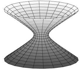
Figure 2: Two-dimensional de Sitter Space. The timelike direction is vertical, and spatial sections are closed. The right-hand diagram shows a null geodesic, which is a straight line in the embedding space.

To establish an analogous picture to the Poincaré disc for de Sitter space, we start by considering the spatial section at $T=0$. This section is a ring of radius $a$, which is mapped onto a straight line in a $(1,1)$ Lorentzian space via a stereographic projection. Null geodesics from this section are now represented as $45^{\circ}$ straight lines in Lorentzian space. Since geodesics from opposite points on the ring meet at infinity, we arrive at a boundary in the timelike direction defined by a hyperbola. This construction provides us with a Lorentzian view of de Sitter geometry. Timelike geodesics in de Sitter space are represented by hyperbolae that intersect the boundary at a right-angle (see figure 3). Here ‘right-angle’ is defined in its Lorentzian sense (the tangent vectors have vanishing Lorentzian inner product). This view has the convenient feature that geodesics are lines of constant Lorentzian distance from some fixed point. The metric associated with this view of de Sitter geometry has the conformal structure

$$ds^{2}=\frac{a^{4}}{(a^{2}+\mathsf{x}^{2}-\mathsf{t}^{2})^{2}}(d\mathsf{t}^{2}-d\mathsf{x}^{2}),$$ (5)

which makes it clear that null geodesics must remain as straight lines in the $\mathsf{x}$–$\mathsf{t}$ plane.

Figure 3: The Lorentzian view of two-dimensional de Sitter space. The boundary is defined by two hyperbolae (shown with thick lines). All geodesics through the origin are straight lines, and null geodesics are always straight lines at $45^{\circ}$. Two further geodesics, one spacelike and one timelike, are also shown. These are hyperbolae which do not pass through the origin. The timelike geodesic intersects the boundary in such a way that the two tangent vectors have vanishing Lorentzian inner product.

There are many fascinating geometric structures associated with de Sitter geometry, many of which mirror those of non-Euclidean geometry. For example, one can always find a reflection that takes any point to the origin [10]. One can then prove a number of results at the origin, where the geodesics are all straight lines, and the results are guaranteed to hold at all points. A similar approach can be applied to anti-de Sitter space, except now the diagram is rotated through $90^{\circ}$, as it is the timelike direction that is formed from a stereographic unwrapping of a circle.

3 Cosmological models and the de Sitter end state

All cosmological models are conformally flat, and can all be interchanged via conformal transformations. Furthermore, all models containing a cosmological constant, and which do not recollapse, will tend towards a de Sitter end. Such models should fit neatly within the conformal diagram of figure 3 with future infinity represented by the upper hyperbolic boundary. There are three cases to consider, for open, closed and flat cosmologies. In this paper we are interested in closed cosmologies, but before looking at these it is informative to consider the other cases. A flat section of de Sitter space corresponds to a region contained within a light cone from a point located on the boundary at past infinity (see figure 4). Surfaces of constant cosmic time are represented as hyperbolae, any one of which can then be chosen to represent the initial singularity. Similarly, an open section of de Sitter space is represented by the area inside a light-cone from a point in the middle of the de Sitter picture. A more general open $\Lambda$-cosmology will have the initial singularity located on a spacelike hyperbola. (See Ratra and Peebles [11] for more details of inflation in open cosmologies.)

Figure 4: Flat and open cosmological models. de Sitter space contains sections representing both flat and open spacetimes. A flat spacetime (left) consists of the space contained inside a light-cone located on past infinity. An open spacetime fits inside the lightcone from the origin. Both pictures can be used to illustrate cosmological models, with the initial singularity represented by a hyperbolic spacelike surface. An example of these surfaces is shown on each diagram.

The diagrams for flat and open cosmologies make it clear that one is not employing the full de Sitter geometry in a symmetric manner. Closed models, on the other hand, have a more natural embedding, with the initial singularity represented by a spacelike surface in the conformal diagram of figure 3. Here we begin to see a natural boundary condition emerging. Suppose that we insist that $\mathsf{t}=0$ represents the initial singularity, so that the entire history of the universe can be conformally mapped into the top half of the de Sitter diagram. (This does not imply that the actual universe is static, it is merely a statement about its conformal representation.) This is certainly the most natural, symmetric place to locate the singularity. An immediate consequence is that any photon emitted from the initial singularity may travel a maximum of precisely one-quarter of the way round the universe in the entire future evolution of the universe. An alternative way of saying this is that the past horizon projected back to $\mathsf{t}=0$ should cover half of the de Sitter geometry.

Given an equatorial angle $\phi$ on a 3-sphere, a photon travelling round the equator will satisfy

$$\frac{d\phi}{dt}=\frac{1}{R},$$ (6)

where $t$ is cosmic time. Traversing the entire universe corresponds to running from $0\leq\phi\leq 2\pi$. If a photon is only to travel one-quarter of the way round we therefore require that

$$\int_{0}^{\infty}\frac{dt}{R}=\int_{0}^{\infty}\frac{dR}{R(-1+\Lambda R^{2}/3+8\pi\rho R^{2}/3)^{1/2}}=\pi/2.$$ (7)

At this point is is useful to define the conformal time $\eta$ by

$$\eta=\int_{0}^{t}\frac{dt^{\prime}}{R(t^{\prime})}.$$ (8)

Note that for closed models the conformal time $\eta$ is not the same as the time-like conformal coordinate $\mathsf{t}$ (see appendix A). Our boundary condition now states that the end of the universe corresponds to a total passing of $\pi/2$ units of conformal time.

The constraint $\eta(\infty)=\pi/2$ can be arrived at through an alternative route that works entirely within the conformal representation of cosmological models, with the line element written in the form

$$ds^{2}=\frac{1}{f^{2}}\bigl{(}d\mathsf{t}^{2}-d\mathsf{x}^{2}-d\mathsf{y}^{2}-d\mathsf{z}^{2}\bigr{)}.$$ (9)

The precise form of $f$ depends on the spatial topology. In appendix A we show that the three cases reduce to

$$f =\frac{\mathsf{t}}{R\sin(\eta)}=g\left(\frac{2\lambda\mathsf{t}}{\lambda^{2}+\mathsf{r}^{2}-\mathsf{t}^{2}}\right)\,\frac{\mathsf{t}}{\lambda}$$ closed

$$f =\frac{2\lambda}{R}$$ flat (10)

$$f =\frac{\mathsf{t}}{R\sinh(\eta)}=\bar{g}\left(\frac{2\lambda\mathsf{t}}{\lambda^{2}+\mathsf{t}^{2}-\mathsf{r}^{2}}\right)\,\frac{\mathsf{t}}{\lambda}$$ open

where $\mathsf{r}^{2}=\mathsf{x}^{2}+\mathsf{y}^{2}+\mathsf{z}^{2}$, $\lambda$ is a constant with dimensions of distance, and the forms of $g$ and $\bar{g}$ depends on the model for the matter content. The coordinate ranges are as illustrated in figures 3 and 4. A de Sitter space centred on $t=0=\mathsf{t}$ has the conformal line element

$$ds^{2}=\frac{12\lambda^{2}}{\Lambda(\lambda^{2}+\mathsf{r}^{2}-\mathsf{t}^{2})}\bigl{(}d\mathsf{t}^{2}-d\mathsf{x}^{2}-d\mathsf{y}^{2}-d\mathsf{z}^{2}\bigr{)}.$$ (11)

Clearly the only solutions that have any chance of matching onto this final state are those for a closed universe. Furthermore, the function $g$ must satisfy

$$\lim_{\chi\mapsto\infty}g(\chi)=\left(\frac{\lambda^{2}\Lambda}{3}\right)^{1/2}\frac{1}{\chi}$$ (12)

where

$$\chi=\frac{2\lambda\mathsf{t}}{\lambda^{2}+\mathsf{r}^{2}-\mathsf{t}^{2}}=\tan(\eta).$$ (13)

But since

$$g=\frac{\lambda}{R\sin(\eta)}$$ (14)

we must then have $R\cos(\eta)$ tending to a constant at large times. This is only possible if $\eta$ tends to $\pi/2$, recovering our earlier boundary condition. This derivation is instructive in that it reveals how the constraint can be imposed as a straightforward boundary condition on a differential equation. In this case, the equation for $g(\chi)$ is

$$\chi^{2}(1+\chi^{2})\left(\frac{dg}{d\chi}\right)^{2}+\frac{d}{d\chi}(g^{2}\chi)=\frac{8\pi G\lambda^{2}\rho}{3}+\frac{\lambda^{2}\Lambda}{3}.$$ (15)

The task then is to solve this equation subject to the boundary condition that $g$ falls off as $1/\chi$ for large $\chi$. Viewed this way the constraint can be thought of as a ‘quantisation condition’ applied as the universe is formed, which one might hope would emerge from a quantum theory of gravity.

In order to understand the implications of our boundary condition, we first write the FRW equations in the form

$$\frac{d\Omega_{\Lambda}}{d\Omega_{M}}=\frac{\Omega_{\Lambda}\bigl{(}(1+3\gamma)\Omega_{M}-2(\Omega_{\Lambda}-1)\bigr{)}}{\Omega_{M}\bigl{(}(1+3\gamma)(\Omega_{M}-1)-2\Omega_{\Lambda}\bigr{)}},$$ (16)

where $\gamma$ encodes the equation of state in the form

$$P=\gamma\rho.$$ (17)

Equation (16) defines a series of flow lines in the $\Omega_{M}$–$\Omega_{\Lambda}$ plane, and also highlights the significance of the points $(1,0)$ and $(0,1)$, which are attractors of the flow lines. This behaviour is illustrated in figure 5, which shows a series of flow lines starting from $\Omega_{M}=1$, $\Omega_{\Lambda}=0$.

\psfrag{Omm}{\small$\Omega_{M}$}\psfrag{Oml}{\small$\Omega_{\Lambda}$}\includegraphics[height=128.0374pt]{flowplt.eps}

\psfrag{Omm}{\small$\Omega_{M}$}\psfrag{Oml}{\small$\Omega_{\Lambda}$}\includegraphics[height=128.0374pt]{radflowplt.eps}

Figure 5: Evolution curves in the $\Omega_{M}$–$\Omega_{\Lambda}$ plane. The left-hand plot is for dust, and the right-hand plot is for radiation. In both cases the curves converge to $\Omega_{\Lambda}=1$, representing a late-time de Sitter phase.

An alternative version of the equations, more useful in describing the universe since recombination, is to assume that the matter density is made up of decoupled dust and radiation. Writing the densities of these as $\rho_{m}$ and $\rho_{r}$ respectively, we introduce the quantities

$$\Omega_{m}=\frac{8\pi G\rho_{m}}{3H^{2}},\quad\mbox{and}\quad\Omega_{r}=\frac{8\pi G\rho_{r}}{3H^{2}}.$$ (18)

Since the matter and radiation are decoupled, both stress-energy tensors satisfy separate conservation laws, which reduce to

$$\rho_{m}R^{3}=\mbox{constant},\quad\mbox{and}\quad\rho_{r}R^{4}=\mbox{constant}.$$ (19)

For this case we find that the equations governing $\Omega_{\Lambda}$, $\Omega_{m}$ and $\Omega_{r}$ can be solved exactly, with the solution governed by two arbitrary constants. We label these $\alpha$ and $\beta$, where

$$\alpha=\frac{\Omega_{m}^{2}\Omega_{\Lambda}}{(\Omega_{m}+\Omega_{r}+\Omega_{\Lambda}-1)^{3}}=\frac{(8\pi G\rho_{m}R^{3})^{2}\Lambda}{27},$$ (20)

and

$$\alpha\beta=\frac{\Omega_{r}\Omega_{\Lambda}}{(\Omega_{m}+\Omega_{r}+\Omega_{\Lambda}-1)^{2}}=\frac{8\pi G\rho_{r}R^{4}\Lambda}{9}.$$ (21)

Present knowledge of $\Omega_{m}$, $\Omega_{r}$ and $\Omega_{\Lambda}$ fixes $\alpha$ and $\beta$, and so picks out a unique curve. The curve will be valid back to last scattering, beyond which the equation of state becomes more complicated.

The diagrams in figure 5 highlight the fact that as the universe evolves the flow lines refocus around the spatially flat case, $\Omega_{M}+\Omega_{\Lambda}=1$. One can show that, for a large range of initial conditions, by the time we reach the current value of $\Omega_{M}\approx 0.3$ most models are not far off spatial flatness. This prediction contrasts with models without a cosmological constant, where any slight deviation from the critical density in the early universe is scaled enormously by the time we reach the present epoch, implying that the parameters in the early universe are highly fine-tuned. One can see the problem straightforwardly by writing

$$\kappa=\Omega_{m}+\Omega_{r}+\Omega_{\Lambda}-1.$$ (22)

The parameter $\kappa$ measures the deviation from spatial flatness, and satisfies

$$\frac{\dot{\kappa}}{\kappa}=H(\Omega_{m}+2\Omega_{r}-2\Omega_{\Lambda}).$$ (23)

If $\Omega_{\Lambda}=0$ the right-hand side is always positive, and nothing prevents the continued growth of $\kappa$. The presence of a $\Lambda$ term changes this completely. At some finite time $2\Omega_{\Lambda}$ will overtake the matter terms, and $\kappa$ is refocused back to $\kappa=0$. The presence of a cosmological constant therefore goes someway to solving the flatness problem on its own, without having to invoke inflation.

\psfrag{Omm}{$\Omega_{M}$}\psfrag{Oml}{$\Omega_{\Lambda}$}\includegraphics[height=170.71652pt]{crit.eps}

Figure 6: Critical paths as predicted by the de Sitter embedding. The solid line represents a matter-dominated universe, and the broken line shows radiation, for comparison. The straight line is the critical case of spatial flatness. By the time we reach $\Omega_{M}\approx 0.3$ the universe has been driven close to critical density.

For the case of a universe filled with non-interacting dust and radiation we can write the boundary condition of equation (7) as

$$\int_{0}^{\infty}\frac{dx}{(\beta x^{4}+x^{3}-x^{2}+\alpha)^{1/2}}=\pi/2.$$ (24)

This equation is therefore an eigenvalue problem for the dimensionless ratios $\alpha$ and $\beta$. For the case of dust ($\beta=0$) the solution turns out to be $\alpha\approx 40.468$. Pinning down a value of $\alpha$ and $\beta$ picks out a unique trajectory in the $\Omega_{M}$–$\Omega_{\Lambda}$ plane. For the straightforward cases of dust ($\beta=0$) and radiation ($\alpha=0$) we arrive at the two curves shown in figure 6. As the universe is expected to be matter dominated for most of its history, the solid line in figure 6 is the more physically relevant one. Taking the present-day energy density to be around $\Omega_{M}=0.3$, we see that $\Omega_{\Lambda}=$ is predicted to be around $\Omega_{\Lambda}\approx 0.83$. That is, a universe that is closed at around the 10% ratio. Such a prediction is reasonably close to the observed value, though it is ruled out by the most recent experiments [1]. In order to improve the prediction, we need to use up a greater fraction of the conformal time before we enter the matter-dominated phase. Such a process is also necessary to solve the horizon problem, and the simplest means of achieving this is via an inflationary phase.

4 Scalar fields and inflation

Much effort has gone into constructing quantum field theories in de Sitter space [12, 13, 14, 15]. There are two reasons why this is more complicated that in Minkowski space: the closed spatial sections give rise to a quantization condition; and the presence of event horizons give rise to ambiguities in the definition of the vacuum. Similar issues can arise when considering an evolving closed universe and will be relevant for a complete treatment of the growth of perturbations seeded by a scalar field. In this section we will ignore such issues, delaying a discussion of the quantization procedure until section 5. Our model for the matter therefore consists simply of a real, time-dependent, homogeneous massive scalar field. For a range of initial conditions this system shows the expected inflationary behaviour. The equations for this model are

$$\dot{H}+H^{2}-\frac{\Lambda}{3}+\frac{4\pi G}{3}(2\dot{\phi}^{2}-m^{2}\phi^{2})=0$$ (25)

and

$$\ddot{\phi}+3H\dot{\phi}+m^{2}\phi=0.$$ (26)

Here $\phi$ has dimensions of $(\mbox{length})^{-1}$, which is the convention widely adopted in the cosmology literature (though this does differ from the relativistic quantum mechanics literature [16]). As stated in the introduction, it is convenient to keep in explicit factors of $G$, to keep the units clear. For closed models the scale factor is given explicitly by

$$\frac{1}{R^{2}}=\frac{4\pi G}{3}(\dot{\phi}^{2}+m^{2}\phi^{2})-H^{2}+\frac{\Lambda}{3}.$$ (27)

Given a solution to the pair of equations (25) and (26), a new solution set is generated by scaling with a constant $\sigma$ and defining

$$H^{\prime}(t)=\sigma{H}(\sigma t),\quad{\phi}^{\prime}(t)={\phi}(\sigma t),\quad m^{\prime}=\sigma m,\quad{\Lambda}^{\prime}=\sigma^{2}{\Lambda}.$$ (28)

This scaling property is valuable for numerical work, as a range of situations can be covered by a single numerical integration. Furthermore, many physically interesting quantities turn out to be invariant under changes in scale. These include the conformal time $\eta$, which is easily confirmed to be scale invariant from equation (8). Invariant quantities such as $\eta$ turn out to be extremely helpful when considering the initial conditions as the universe emerges from the big bang. The scaling property does not survive quantisation, however, so has to be employed carefully when considering vacuum fluctuations.

The initial conditions for equations (25) and (26) are usually set at the start of the inflationary period, where they are viewed as arising from some form of quantum gravity interaction. But in order to apply our boundary condition we need to track the equations right back to the initial singularity, as this is the only way that we can keep track of the total conformal time that has elapsed. As we argue below, evolving the inflationary equation backwards in time is entirely justified, as we do not expect quantum gravity to play a role until much earlier in the history of the universe. Inflation on its own does not eliminate singularities from cosmology [17]. Our approach has the added benefit that the conditions at the start of inflation are fully determined by a pair of parameters, making the model highly predictive.

As the universe emerges from the big bang the dominant behaviour of $H$ is to go as $1/(3t)$. Equation (25) then implies that $\phi$ must contain a term going as $\ln(t)$. But this in turn implies that $H$ must also contain a term in $t\ln(t)$, in order to satisfy equation (26). Working in this manner we conclude that a series expansion in terms of $\ln(t)$ is required to describe the behaviour around the singularity. At this point it is convenient to define the dimensionless variables

$$u=\frac{t}{t_{p}},\qquad\mu=\frac{m}{m_{p}}$$ (29)

with $t_{p}$ and $m_{p}$ the Planck time and mass respectively. The series expansion about the singularity at $t=0$ can now be written

$${H}(u) =\frac{1}{t_{p}}\sum_{i=0}^{\infty}H_{i}(u)\ln^{i}(u)$$ (30)

$${\phi}(u) =\frac{1}{l_{p}}\sum_{i=0}^{\infty}\phi_{i}(u)\ln^{i}(u),$$ (31)

which ensures that the expansion coefficients are all dimensionless. Substituting these into the two evolution equations, and setting each coefficient of $\ln(u)$ to zero, we establish that

$$H_{1} =-u\frac{dH_{0}}{du}-uH_{0}^{2}+\frac{u{\Lambda}}{3}-\frac{8\pi u}{3}\left(\frac{d\phi_{0}}{du}\right)^{2}-\frac{16\pi\phi_{1}}{3}\frac{d\phi_{0}}{du}$$

$$\quad-\frac{8\pi\phi_{1}^{2}}{3u}+\frac{4\pi\mu^{2}u\phi_{0}^{2}}{3},$$ (32)

with further algebraic equations holding for $H_{2},\phi_{2}$, $H_{3},\phi_{3}$, and so on. So, by specifying $H_{0}$, $\phi_{0}$ and $\phi_{1}$, all the remaining terms in the solution are fixed. The aim then is to choose the three input functions to ensure that successive terms in the series get progressively smaller. This turns out to provide just the right number of equations to specify all coefficients, save for two arbitrary coefficients in $\phi_{0}$. The end result is a series controlled entirely by a pair of arbitrary constants: the expected number of degrees of freedom once we have fixed the singularity to $t=0$. In order to generate curvature it turns out that the input functions need to be power series in $u^{1/3}$, which ensures that the scale factor goes as $u^{1/3}$ at small times. The series solution is only required to find suitable initial conditions for numerical evolution, so only the first few terms are required. Expanding up to order $u^{5/3}$ we find that

$$H_{0} =\frac{1}{3u}+\frac{32\sqrt{3\pi}}{27}b_{4}u^{1/3}$$

$$\quad+\left(\frac{2\mu^{2}}{81}+\frac{{\Lambda}}{3}+\frac{4\pi}{3}\mu^{2}b_{0}^{2}+\frac{4\sqrt{3\pi}}{27}{\mu}^{2}b_{0}\right)u-\frac{6656\pi b_{4}^{2}}{891}u^{5/3},$$ (33)

$$\phi_{0} =b_{0}+b_{4}u^{4/3}-\frac{118\sqrt{3\pi}b_{4}^{2}}{99}u^{8/3}$$

$$\quad-\frac{1}{1296\pi}\left(11\sqrt{3\pi}\mu^{2}-54\sqrt{3\pi}{\Lambda}-216\sqrt{3}\,\pi^{3/2}\mu^{2}b_{0}^{2}+36\pi\mu^{2}b_{0}\right)u^{2}$$ (34)

and

$$\phi_{1}=-\sqrt{\frac{1}{12\pi}}-{\frac{\mu^{2}}{216\pi}}\left(-\sqrt{3\pi}+36\pi b_{0}\right)u^{2}.$$ (35)

Under scaling the three key parameters in the model transform as

$$\mu\mapsto\sigma\mu,\qquad b_{0}\mapsto b_{0},\qquad b_{4}\mapsto\sigma^{4/3}b_{4}.$$ (36)

The scaling transformation for $b_{4}$ is entirely as expected, given that it is the coefficient of $u^{4/3}$ in the series for $\phi_{0}$. It follows that the quantity $b_{4}/\mu^{4/3}$ is scale invariant.

Figure 7: Hubble function entry into the inflationary regime. The Hubble function emerges from the big bang going as $1/3t$. As $H$ falls it quickly enters the inflationary region, during which it falls linearly. Time $t$ is measured in units of $t_{p}$, and $H$ in units of $t_{p}^{-1}$. The input parameters were set to $b_{0}=2.48$, $b_{4}=-0.51$ and $m=m_{p}$ ($\mu=1$). These values of $b_{0}$ and $b_{4}/\mu^{4/3}$ are illustrative of physically realistic models. The cosmological constant term has no effect in this region and can be set to zero.

The plot in figure 7 illustrates the general behaviour around the initial singularity. As the universe emerges from the big bang the energy density in the scalar field is dominated by the $\dot{\phi}$ term, and the field behaves as if it is massless. It follows that $H$ initially falls as $1/(3t)$. But once $H$ has fallen sufficiently far we enter a region in which $m^{2}\phi^{2}$ starts to dominate over $\dot{\phi}^{2}$. These are suitable initial conditions for the universe to enter an inflationary phase. By varying $b_{0}$, $b_{4}$ and $\mu$ we control both the values of the fields as we enter the inflationary period, and how long the inflationary period lasts. The cosmological constant plays no significant role in this part of the evolution. The dynamics displayed in this figure is quite robust over a range of input parameters.

The fact that $b_{4}$ controls the curvature can be seen from equation (27) which, to leading order, yields

$$\frac{R}{l_{p}}=\frac{1}{\mu}\left(\frac{2187}{12544\pi}\right)^{1/4}\left(-\frac{\mu^{4/3}}{b_{4}}\right)^{1/2}(\mu u)^{1/3}+\cdots.$$ (37)

Clearly, the arbitrary constant $b_{4}$ must be negative for a closed universe. The terms on the right-hand side of equation (37) are all scale invariant, apart from the first factor of $\mu^{-1}$. From figure 7 we can see that, for the typical values of $b_{0}$ and $b_{4}/\mu^{4/3}$ of interest, the onset of inlation corresponds to $\mu u\approx 0.1$. As we discuss below, in order to generate perturbations consistent with observation the scalar field must have a low mass, with $\mu$ of the order of $10^{-6}m_{p}$. It follows that the onset of inflation occurs at a time of around $10^{5}$ Planck times. Furthermore, the radius of the universe at the onset of inflation is given approximately by

$$R\approx\frac{0.2}{\mu}l_{p},$$ (38)

and is of order $10^{5}$ Planck lengths. Inflation therefore starts at an epoch well into the classical regime. Quantum gravity effects would be expected to be relevant when the radius of the universe is of the order of the Planck scale, which occurs when $u\approx\mu^{2}$ and is well before any inflationary period (for physical values of $\mu$). We are therefore quite justified in running the evolution equations back past the inflationary regime, and right up to near the initial singularity. It is only when $R=l_{p}$ that the equations will break down, and we would look to quantum gravity to explain the formation of the initial, Planck-scale sized universe. We might hope here that quantum gravity will provide a probability distribution for the two classical parameters controlling the evolution of the scalar field. Furthermore, we can argue more strongly that we have to run the equations backwards in time to well before the start of inflation before reaching an epoch where new physics could be expected to enter the problem.

As the universe is described by a 3-sphere of radius $R$, the total volume of the universe is given to leading order by

$$V=2\pi^{2}\left(\frac{2187}{12544\pi}\right)^{3/4}\frac{l_{p}^{3}}{(-b_{4})^{3/2}}u+\cdots.$$ (39)

Following from this, an interesting calculation we can perform in a closed universe is to find the total energy contained within it in the scalar field. By integrating the energy density we find that

$$E_{\mbox{tot}}=\frac{\pi}{12}\left(\frac{2187}{12544\pi}\right)^{3/4}\frac{1}{(-b_{4})^{3/2}}\frac{\hbar}{t}+\cdots\approx 0.03\left(\frac{-\mu^{4/3}}{b_{4}}\right)^{3/2}\frac{\hbar}{\mu^{2}t}.$$ (40)

We return to a discussion of this equation in section 7.

Figure 8: Hubble function exit from the inflationary regime. As the inflationary era ends the density and pressure start oscillating around values for a matter-dominated cosmology. The effective singularity for this dust cosmology is displaced from $t=0$. The broken line plots the natural log of $2/3(t-14.56)$. The parameters in this model are $b_{0}=2.48$, $b_{4}=-0.51$ and $m=m_{p}$.

The typical behaviour as we exit the inflationary region is shown in figure 8. The end of inflation is characterised by ${H}\approx\mu$. Beyond this point the scalar field enters an oscillatory phase, with the time-averaged fields satisfying the conditions for a simple matter-dominated cosmology. In this case $H$ can be approximated by a curve going as $2/3(t-t_{0})$, describing a dust model with a displaced origin. The universe then appears as if it has been generated by a big bang at a later time. We call this the effective big bang. Of course, around this time we expect reheating effects to start to dominate, so that in reality the universe must pass over to a radiation-dominated era. However, the naive ‘effective big bang’ concept is useful for extracting some qualitative predictions from our model.

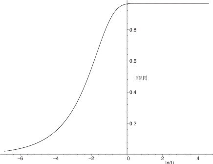
Figure 9: Evolution of the conformal time $\eta(t)$ as a function of $\ln(t)$. The parameters for the model are as given in figure 8 and again $t$ is measured in units of the Planck time. This plot sets $\mu=1$, so the time variable must be scaled to correspond to more physical values of $\mu\approx 10^{-6}$.

As well as giving a new effective start time for the big bang, inflation must also resolve the horizon problem. The conformal picture provides a straightforward means of visualising this process. The key is to compute how much conformal time has elapsed by the end of the inflationary era. Using the same parameters as in figure 8 we find that the conformal time evolves as shown in figure 9. As the universe emerges from the (real) big bang $\eta$ initially grows at $t^{2/3}$, as can be seen from equation (37). This gives rise to the rapid growth seen in figure 9, which plots $\eta$ as a function of $\ln(t/t_{p})$. But once the inflationary region is entered, $R(t)$ starts to increase rapidly. So the conformal time, which involves the time integral of $R^{-1}$, quickly saturates, as can also be seen in figure 9. Any further increase in $\eta$ will take an extremely long time to occur, since the integrand $1/R$ is extremely small. So if $\eta$ has not reached $\pi/2$ before $R$ has inflated significantly, the universe will have to exist for an extremely long time to reach the boundary value of $\pi/2$.

For the parameters used in figures 8 and 9 we can see that $\eta$ saturates at a value of around 0.97 by the end of inflation (at around $t=100t_{p}$). The value of $R$ at this time is $2\times 10^{22}\mu^{-1}l_{p}$. All changes in $\eta$ beyond the end of inflation occur very slowly. Irrespective of the properties of the reheating phase, $\eta$ will have changed very little by the time recombination occurs. This pushes the era of recombination to a much later conformal time, close to the value for the present epoch. This removes the horizon problem, as the obervable patch of the universe has been in causal contact and has had sufficient time to thermalise (see figure 10). This is not true of the universe as a whole, as antipodal points remain outside each other’s light cone until $t=\infty$.

Figure 10: The horizon problem for a closed universe in the conformal picture. The lower solid line represents the surface of last scattering, and the broken line just above it is the current epoch. The thick line is the future boundary ($t=\infty$). Null geodesics lie at $45^{\circ}$, so there is no problem with points in the observable part of the surface of last scattering having once been in causal contact.

In order to make some initial estimates from our boundary condition, we will ignore the effects of reheating and nucleosynthesis, and assume that the universe just smoothly enters a matter-dominated phase described by

$$R=R_{1}\left(\frac{t-t_{0}}{t_{1}-t_{0}}\right)^{2/3}.$$ (41)

For the parameters we are currently considering we have $R_{1}=2\times 10^{22}l_{p}$, $t_{0}=14.56t_{p}$ and $t_{1}=100t_{p}$. We will also ignore the cosmological constant, though this will clearly affect the behaviour at late times. The conformal time elapsed at some later cosmic time $t$ can be approximated by

$$\eta\approx\eta(t_{1})+\frac{3}{R_{1}}(t-t_{0})^{1/3}(t_{1}-t_{0})^{2/3}\approx 0.97+2.4\times 10^{-19}\,t^{1/3},$$ (42)

where $t$ is measured in units of the Planck time. We can therefore arrive at a crude estimate for the age of the universe simply by setting $\eta=\pi/2$. This gives a time of $1.6\times 10^{61}$ in Planck units, or about $2.8\times 10^{10}$ years. This is a good illustration of how some very large numbers (such as the age of the universe in Planck times) can emerge from a simple model of inflation, augmented with our closed universe boundary condition.

In order to produce a more detailed prediction, we return to considering trajectories in the $\Omega_{M}$–$\Omega_{\Lambda}$ plane. We can still assume that the universe is essentially matter dominated throughout its history, but now the total amount of conformal time that should elapse along the trajectory is less than $\pi/2$. The effect of this is to drive us onto trajectories which are closer to the critical line. If we only require a total conformal time of around 0.6 to elapse during the matter-dominated phase of the universe (as for the model above), then we require an $\alpha$ value of around $10^{4}$, producing a trajectory that is very close to spatially flat, and predicting a universe which is currently closed at around the $1\%$ level (see figure 11).

\psfrag{Omm}{$\Omega_{M}$}\psfrag{Oml}{$\Omega_{\Lambda}$}\includegraphics[height=227.62204pt,angle={-90}]{MLpltwitheta.eps}

Figure 11: Matter-dominated trajectory in the $\Omega_{M}$–$\Omega_{\Lambda}$ plane. The trajectory (solid line) is picked out by demanding that the total conformal time elapsed throughout the evolution is 0.6. This evolution joins onto an inflationary model which takes up around 0.97 units of conformal time, so that the boundary condition of a total of $\pi/2$ is obeyed.

We can now see that our boundary condition gives rise to a remarkable see-saw mechanism, with two key components. The first component relates to the amount of inflation that occurs. For a range of conditions, the time at which inflation starts can be approximated by

$$u_{i}=\frac{1}{(12\pi)^{1/2}\mu b_{0}}.$$ (43)

A check on the physical approximations we make here is that this quantity has the correct scale transformation properties under the transformation of equation (36). The value of ${H}$ at the start of slow-roll inflation can be approximated by $1/(3u_{i})$,

$${H}_{i}=\frac{1}{3u_{i}},$$ (44)

and a suitable condition for the end of slow roll can be taken as

$${H}_{f}^{2}=\frac{\mu^{2}}{3}.$$ (45)

During slow roll the evolution of ${H}$ is well approximated by a linear fit, so

$${H}={H}_{i}-\frac{u-u_{i}}{u_{f}-u_{i}}({H}_{i}-{H}_{f}).$$ (46)

The gradient is determined from the field equations to be

$$\frac{{H}_{i}-{H}_{f}}{u_{f}-u_{i}}=\frac{\mu^{2}}{3}.$$ (47)

The total number of e-foldings, $N$, can therefore be approximated by

$$N=\int_{u_{i}}^{u_{f}}\!\!{H}\,du\approx\frac{3}{2\mu^{2}}({H}_{i}^{2}-{H}_{f}^{2})\approx 2\pi b_{0}^{2}.$$ (48)

Numerical simulations reveal that this approximation does give a correct order-of-magnitude for the number of e-foldings, though it does tend to underestimate the precise value. As expected, the result for $N$ is invariant under scale changes, as is clear from the integral formula for $N$. The key conclusion is that the number of e-foldings is primarily determined by $b_{0}$, with the value of $H$ at the end of inflation fixed by $\mu$. The value of $b_{4}$ essentially decouples from $N$. An increase in $b_{0}$ leads to an increase in the final value of $R$, and hence to an increase in $\rho R^{3}$ in the matter phase. From equation (20) we see that, in order to preserve $\alpha$, any increase in $\rho R^{3}$ must be offset by a decrease in the cosmological constant. Conversely, the observed value of $\Lambda$ can be employed to constrain the amount of inflation.

The second quantity of interest, given our boundary condition, is the amount of conformal time that has elapsed before the universe enters the present matter-dominated epoch. Figure 9 shows the typical evolution of $\eta$. We see that a large percentage of the conformal time is taken up before inflation starts. During this region we can approximate $R$ by equation (37). Taking $u_{i}$ as roughly approximating the point where $\eta$ starts to saturate, we find that the conformal time that has elapsed is approximated by

$$\eta=\int_{0}^{u_{i}t_{p}}\frac{dt}{R}\approx 0.92\left(\frac{|b_{4}|}{\mu^{4/3}}\right)^{1/2}\left(\frac{1}{b_{0}^{2}}\right).$$ (49)

And again, the result naturally assembles into a scale-invariant quantity. This result typically underestimates the total elapsed $\eta$ at the end of inflation, but it does set a useful restriction on the order of magnitude of the expression on the right-hand side. We now see that, for fixed $b_{0}$ and $\mu$, the greater the initial curvature (increasing $|b_{4}|$), the greater the amount of conformal time taken up during inflation. This in turn forces the universe today to be closer to flat. And conversely, the more spatially curved we want the universe to be today, the closer to flat it must be initially. This is the second component of the see-saw mechanism. The observed values of the cosmological parameters, together with our boundary condition, therefore place a severe restriction on the allowed models.

Given the strong constraints our model places on trajectories in the $\Omega_{M}-\Omega_{\Lambda}$ plane, the model must predict the small value of the cosmological constant. To see how small values of $\Lambda$ naturally arise, we return to equation (20) and write

$$\Lambda=\frac{27\alpha}{(8\pi G\rho_{m}R^{3})^{2}}.$$ (50)

In order to make some useful approximations we will again ignore the effects of reheating and radiation domination, and simply assume that $\rho_{m}R^{3}$ is given by its value for the scalar field at the end of inflation. If we furthermore ignore the effects of curvature and $\Lambda$ at this stage, we can write $8\pi G\rho_{m}=3H^{2}$, so we have

$$\Lambda=\left.\frac{3\alpha}{H^{4}R^{6}}\right|_{\mathrm{end}}.$$ (51)

This expression does not depend on the precise moment of evaluation. As we have seen, typical values of $\alpha$ are in the range $10^{3}$ to $10^{5}$. The small value of $\Lambda$ is therefore seen to be a consequence of the large values of $RH^{2/3}$ achieved by the end of inflation. The value of $H$ at the end of inflation is given by equation (45), and for $R$ at the end of inflation, $R_{f}$, we can write

$$R_{f}=e^{N}R_{i}.$$ (52)

Here $R_{i}$ is the value of $R$ at the start of inflation, and $N$ is the number of e-foldings. We can estimate $R_{i}$ using equation (37) and the value of $u_{i}$ from equation (43). Putting these together, we arrive at the approximate formula

$$\Lambda\approx 8\times 10^{4}\alpha\frac{|b_{4}|}{\mu^{4/3}}b_{0}^{2}\mu^{2}e^{-6N}l_{p}^{-2}.$$ (53)

The typical models we consider have $N$ in the range of 40 to 50, and $\mu$ around $10^{-6}$, which does indeed predict an extremely small value for the cosmological constant. As commented in the introduction, the dominant behaviour in $\Lambda$ is governed by the $\exp(-6N)$ term, which immediately yields values for $\Lambda$ of the expected magnitude.

5 The curvature spectrum

Our proposed ‘quantisation’ condition on the available conformal time places a strong restriction on the class of allowed models. We must now see whether any of these models produce a perturbation spectrum consistent with the observed primordial fluctuations in the CMB. Due to the scale-invariant nature of the equations (under the transformation of equation (28)), the parameters that determine the key features of the inflationary period are the scale-invariant quantities $b_{0}$ and $b_{4}/\mu^{4/3}$. Furthermore, the restriction that the total amount of conformal time available is $\pi/2$ constrains the combination in equation (49) to be of order 1. This limits us to a highly restricted class of models.

The scale transformation we have utilised at various points is not conserved by quantisation, so vacuum fluctuations impose an absolute scale on the model. The key quantity that determines the size of the perturbations is the mass ratio $\mu=m/m_{p}$. For models with a quadratic potential to generate perturbations consistent with observation we need to set $\mu$ to be around $10^{-6}$. As explained above, this value is irrelevant for the evolution of the scalar field, but $\mu$ does set the absolute size of the Hubble function, and so fixes the magnitude of perturbations.

In order to consider a concrete example, we adopt the following set of parameters:

$$b_{0}=2.37,\qquad\frac{b_{4}}{\mu^{4/3}}=-0.49,\qquad\mu=2.1\times 10^{-6}.$$ (54)

These values are typical for giving good agreement with experiment for the curvature spectrum. Evidently, little fine tuning is required in chosing the two scale-invariant combinations, both of which are of order unity. Furthermore, the predictions we make here are quite robust under variations of these parameters. We are a long way removed from areas of parameter space where chaotic dynamics of the type considered by Cornish & Shellard [18] could prove significant.

In a closed universe model there are two scales of interest: the horizon size $1/H$, and the radius of the spatial sections $R$. The ratio of these defines the dimensionless quantity $1/(RH)$, which is related to the closure density by

$$\Omega-1=\frac{1}{(RH)^{2}},$$ (55)

where the total $\Omega$ is defined by

$$\Omega=\Omega_{\Lambda}+\Omega_{M}.$$ (56)

During inflation $\Omega$ should decrease, as the universe is driven towards flatness. This effect can be seen for our chosen parameters in figure 12, which confirms that the universe is accelerating over the range $e^{11}<t/t_{p}<e^{16}$. The plot also shows that the radius is always greater than the horizon size, which is important when considering perturbation modes.

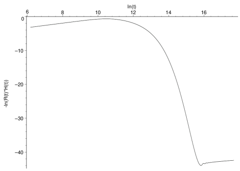
Figure 12: Evolution of $1/(RH)$. The natural log of the dimensionless ratio of the Hubble radius to the curvature radius is plotted against log time (in units of $t_{p}$). The parameters for the model are as described in the text. During the inflationary period, $1/(RH)$ is a decreasing function of time, corresponding to an accelerating phase.

The evolution of the scale factor for our chosen parameters is shown in figure 13. During the inflationary region $\ln(R)$ increases from about 14 to 60. This corresponds to a total number of e-foldings of 46, as expected given our choice of parameters. This is roughly the figure we expect for the number of e-foldings if the universe departs from flatness by an amount that is visible today [5]. In order to give rise to the observed fluctuation spectrum it is thought that around 40–50 e-foldings are required between the point where the present horizon scale leaves the horizon and the end of inflation [19]. For this to hold, we therefore require that the present horizon scale leaves the Hubble horizon soon after the onset of inflation.

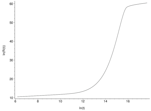
Figure 13: Evolution of the scale factor. The evolution of logarithm of the scale factor $R/l_{p}$ is shown as a function of log time ($t$ in units of $t_{p}$).

Closed universe models have an advantage over flat models when discussing scales and perturbations, because equation (55) gives a direct expression for $R$ in terms of $\Omega$ and $H$. To apply this, suppose that at the current epoch a given physical size occupies a fraction $x$ of the Hubble horizon $1/H_{0}$. The corresponding physical scale is

$$d_{0}=\frac{x}{H_{0}},\quad 0<x<1.$$ (57)

For wave modes, $d_{0}$ will be quantised in units of $2\pi R_{0}/(n^{2}-1)^{1/2}$, where $n$ is an integer. We will ignore this quantisation effect here, as the number of modes available ensure that a continuum is a reasonable approximation for all but the low-$k$ modes. Now consider the distance corresponding to $d_{0}$ in an epoch when the scale factor is $R$ instead of $R_{0}$. This scale is simply $Rx/(R_{0}H_{0})$. This distance is equal to the Hubble horizon at the epoch corresponding to $R$ when

$$\frac{Rx}{R_{0}H_{0}}=\frac{1}{H}.$$ (58)

(As is standard practice we formulate the conditions for horizon crossing in terms of the Hubble horizon, as opposed to the particle horizon.) It follows that the scale corresponding to a given $x$ crosses the Hubble horizon when

$$x=\frac{R_{0}H_{0}}{RH}=\frac{\sqrt{\Omega-1}}{\sqrt{\Omega_{0}-1}}.$$ (59)

So as $\Omega$ is driven to unity during inflation, progressively smaller scales cross the horizon as time advances.

Figure 14 shows the behaviour of $\Omega$ in our scalar field model. As expected, $\Omega$ is driven close to 1 in the region $e^{11}<t/t_{p}<e^{16}$. In order to use this plot in conjunction with equation (59) we need to assign a value to $\Omega_{0}$. The most recent results from WMAP, with all data folded in, give a value of $\Omega_{0}=1.02\pm 0.02$ [1], so here we work with a value of $\Omega_{0}=1.02$. The scale corresponding to the present horizon size ($x=1$) is therefore obtained during inflation when $\Omega=1.02$. Figure 14 shows that this occurs at $\ln(t/t_{p})=12.0$. By reference to figure 13, we see that this time corresponds to roughly 2 e-foldings. This leaves roughly 44 e-foldings to the end of inflation, which are sufficient to produce a fluctuation spectrum with the desired properties. These values are consistent with the estimates of Uzan, Kirchner & Ellis. [6].

Figure 14: Evolution of the total $\Omega$ during inflation. The total density is quickly driven close to flat, after which $\Omega$ only changes slowly.

Each value of $x$ less than 1 corresponds to a scale which leaves the Hubble horizon at successively smaller values of $\Omega$. A remarkable feature of the approach outlined here is that it does not require any knowledge of the evolution of the universe to relate scales today to scales at the end of inflation. This is because in any closed (or non-flat) universe it is possible to measure $R$ directly. This cannot be done if the universe is assumed to be flat throughout inflation, as one loses the ability to track scales through the evolution of $\Omega$. In flat models the only way to find the scale ratio $R/R_{0}$ is to evolve the scale factor $R$ through the history of the universe, including the epoch of reheating, about which little is known. Of course, our method would be impossible to apply if the value of $\Omega_{0}$ turns out to be undetectably close to 1. This is predicted by approaches such as chaotic inflation, which can typically allow of order $10^{10}$ e-foldings [19]. But for models that allow $\Omega_{0}$ to deviate measurably from 1 the method we have outlined here should be of considerable use in calculating the fluctuation spectrum induced by inflation.

In order to compute the primordial curvature spectrum we adopt the slow-roll approximation, following the presentation of Liddle & Lyth [19]. For a quadratic potential, the slow roll condition can be expressed simply in terms of the single parameter $\epsilon$, where

$$\epsilon=\frac{1}{4\pi\phi^{2}}.$$ (60)

For slow roll to hold we require that $\epsilon\ll 1$. However, the model we consider here has $\epsilon$ in the range from $10^{-2}$ to $10^{-1}$, with the larger values corresponding to higher $k$ values. We are therefore close to the point where slow roll ceases to be a good approximation. A concrete example of this is seen when we consider the spectral index (see also Martin & Schwarz [20] for a discussion of the precision of slow roll). For the main evolution of $\phi$, however, plots such as figure 7 confirm that the slow roll approximations are holding up, with the evolution of $H$ roughly linear with the expected gradient of $\mu^{2}/3$. A further source of error, as stated earlier, is that we are ignoring the quantisation effects implied by a closed cosmology. But, despite these provisos, we may hope that the simple, slow-roll equations will still give a reasonably accurate prediction for the curvature spectrum.

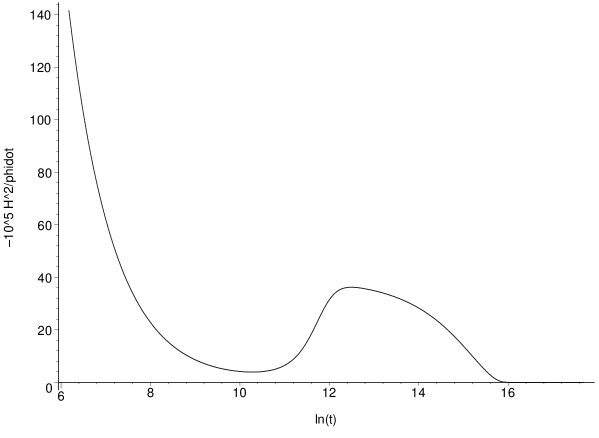
Figure 15: Evolution of $H^{2}/\dot{\phi}$ during inflation. The function plotted is $-10^{5}H^{2}/\dot{\phi}$ as a function of $\ln(t/t_{p})$. This function controls the magnitude of the curvature perturbation.

Given the slow roll approximations, the key equation determining the curvature spectrum ${\mathcal{P}}_{\mathcal{R}}(k)$ is [19]

$${\mathcal{P}}_{\mathcal{R}}(k)=\left(\frac{H}{\dot{\phi}}\right)^{2}\left(\frac{H}{2\pi}\right)^{2},$$ (61)

where the right-hand side is evaluated when a given scale $x$ crosses the horizon. If we write

$${\mathcal{P}}_{{\mathcal{R}}}^{1/2}(k)=\frac{-H^{2}}{2\pi\dot{\phi}}$$ (62)

we see that the power spectrum is controlled by the ratio $H^{2}/\dot{\phi}$. This function is plotted in figure 15. Figures 14 and 15 contain all of the information required to extract ${\mathcal{P}}_{\mathcal{R}}(k)$. Given a comoving wavenumber $k$, we find $x$ from

$$\frac{1}{k}=\frac{x}{H_{0}}.$$ (63)

The value of $x$ is converted to a time using equation (59) and the relationship plotted in figure 14. With the value of $t$ then found, we can read off the spectrum from figure 15. The fact that the graph turns over for $\ln(t/t_{p})<12$ suggests that the spectrum will contain less power at low-$k$ values than would be expected from a straightforward power law in a flat cosmology, in contrast to the predictions of Starobinsky [5]. But again, more detailed calculations are required to confirm this point.

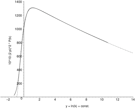
Figure 16: The power spectrum of curvature perturbations. The function plotted is $10^{10}(2\pi)^{2}{\mathcal{P}}_{\mathcal{R}}(k)$ as a function of $y=ln(1/x)=\ln(k)+\mathrm{constant}$. The solid line represents the numerical predictions from our model, and the broken line is the best-fit power law with an exponential cutoff. The parameters are described in the text.

It is convenient to plot perturbation spectra as a function of $y=\ln(1/x)$. With dimensions reinserted, $y$ is given by

$$y=\ln\left(\frac{k}{h}\times 3\times 10^{3}\right)$$ (64)

where $k$ is measured in $\mathrm{Mpc}^{-1}$ and the Hubble constant is given by $H_{0}=100h\mathrm{\,km\,s^{-1}}{\rm\,Mpc^{-1}}$. In figure 16 we plot the power spectrum as a function of $y$ for our chosen parameters, including $\Omega_{0}=1.02$. (For a plot showing the power spectrum as an explicit function of $k$ in $\mathrm{Mpc}^{-1}$ see figure 17.) The quantity plotted (solid curve) is $10^{10}(2\pi)^{2}{\mathcal{P}}_{\mathcal{R}}(k)$. The graph shows a clear cutoff at low-$k$ values. A cutoff of this type was proposed on phenomenological grounds by Efstathiou [21]. Indeed, it turns out that the type of exponential cutoff proposed by Efstathiou agrees remarkably well with our calculations, as can be seen in the dashed line, which plots

$$10^{5}\,2\pi\,\mathcal{P}^{1/2}(k)=37.6(1-.023\,y)(1-\exp(-(y+0.93)/0.47)),$$ (65)

valid for $y>-0.93$. The fact that our model predicts a spectrum which has already been argued for on phenomenological grounds is very reassuring. We can now see that our model will produce a deficit in the CMB power spectrum at low $\ell$, and in section 6 we confirm that this is the case.

Figure 16 contains a further surprise. From equation (65) we see that at large $k$ the relationship between ${\mathcal{P}}_{\mathcal{R}}^{1/2}(k)$ and $\ln(k)$ is roughly linear, which is quite different from the expected power law relation. To understand why this is the case we return to the slow roll equations and derive the form of the spectrum for a quadratic potential, following section 7.5 of Liddle and Lyth [19]. The main relation we require relates the derivatives with respect to $k$ and $\phi$:

$$\frac{d}{d\ln k}=-\frac{1}{4\pi\phi}\frac{d}{d\phi},$$ (66)

where we specialise to results for a quadratic potential. During slow roll the following approximate relations hold:

$$H^{2}=\frac{4\pi}{3}\mu^{2}\phi^{2},\qquad\dot{\phi}=\frac{\mu}{\sqrt{12\pi}}.$$ (67)

It follows that the curvature spectrum is approximated by

$${\mathcal{P}}_{\mathcal{R}}^{1/2}(k)=4\left(\frac{\pi}{3}\right)^{1/2}\mu\phi^{2}.$$ (68)

We therefore find that

$$\frac{d}{d\ln k}{\mathcal{P}}_{\mathcal{R}}^{1/2}(k)=-\frac{2\mu}{\sqrt{3\pi}}.$$ (69)

This confirms that the relationship between ${\mathcal{P}}_{\mathcal{R}}^{1/2}(k)$ and $\ln(k)$ is indeed linear. Furthermore, the gradient is predicted to be $-2\mu/\sqrt{3\pi}$. For the model we are considering this evaluates to $1.35\times 10^{-6}$, which agrees well with the fit of equation (65), which has a gradient of $37.6\times 0.023/(2\pi\times 10^{5})=1.37\times 10^{-6}$. We can also see that

$$\frac{d}{d\ln k}\ln({\mathcal{P}}_{\mathcal{R}}(k))=-2\frac{1}{{\mathcal{P}}_{\mathcal{R}}^{1/2}(k)}\frac{2\mu}{\sqrt{3\pi}}=-\frac{1}{\pi\phi^{2}}=-4\epsilon$$ (70)

where $\epsilon$ is the slow-roll parameter of equation (60). The typical slow-roll approximation is to now write ${\mathcal{P}}_{\mathcal{R}}(k)\propto k^{-4\epsilon}$, so that

$${\mathcal{P}}_{\mathcal{R}}^{1/2}(k)\approx Ak^{-2\epsilon}\approx A(1-2\epsilon\ln(k)+2\epsilon^{2}\ln^{2}(k)+\cdots).$$ (71)

The higher order terms here are incorrect, and introduce an error of order $\epsilon\ln(k)$ to the power spectrum. As commented earlier, at high-$k$ values $\epsilon$ is in the range $0.01$–$0.1$, so this deviation can become quite significant.

In figure 17 we compare our computed scalar power spectrum with the best fit power law ($n_{s}=0.96$) and the WMAP running spectral index best fit. The vertical normalisations for these fits have been chosen arbitrarily, since it is the shape of the spectrum at large $k$ which is of greatest interest here. The WMAP running spectral index model shape is given by

$${\mathcal{P}}_{\mathcal{R}}(k)={\mathcal{P}}_{\mathcal{R}}(k_{0})\exp\left((n_{s}-1)\ln(k/k_{0})+\frac{1}{2}n_{\rm run}(\ln(k/k_{0}))^{2}\right).$$ (72)

Using the WMAP figures for combined data sets their best fit values are $n_{s}=0.93$, $n_{\rm run}=-0.031$ and $k_{0}=0.05{\rm\,Mpc^{-1}}$ [1]. The running spectral index graph is interesting in that it suggests that this model is attempting to emulate both the cutoff at low $k$, as well as the reduced power at large $k$. The latter is possibly required as the strict power law spectrum at large $k$ appears to over-predict the abundance of dwarf galaxies. This is discussed further in section 6.

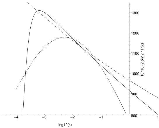
Figure 17: Comparison of the scalar power spectrum with power law models. The function plotted is $10^{10}(2\pi)^{2}{\mathcal{P}}_{\mathcal{R}}(k)$ as a function of $\log_{10}(k)$, assuming $h=0.65$. The solid line represents the numerical predictions from our model. The long dashes represent the best fit power law ($n_{s}=0.96$) and the short dashes are the WMAP running spectral index best fit. Notice that the vertical scale runs from 800 to 1300, so the differences are slightly exaggerated.

A further quantity of interest is the tensor spectrum, which is significant in searches for B-mode polarisation in the CMB. As our definition of the tensor spectrum we take

$${\mathcal{P}}_{\mathrm{grav}}(k)=\frac{16}{\pi}H^{2},$$ (73)

where again the right-hand side is evaluated as the scale controlled by $x$ crosses the horizon. (Here we follow the convention of Martin & Schwarz [20]). The main quantity of interest is the ratio of the tensor and scalar modes $r$,

$$r=\frac{{\mathcal{P}}_{\mathrm{grav}}}{\mathcal{P}_{{\mathcal{R}}}},$$ (74)

where the right-hand side is evaluated at some suitable low $k$. Following the slow-roll approximation, we can write

$$\mathcal{P}_{\rm grav}(k)=\frac{64\mu^{2}\phi^{2}}{3}.$$ (75)

Applying $d/(d\ln k)$ to this now yields

$$\frac{d}{d\ln k}\mathcal{P}_{\rm grav}(k)=-\frac{32\mu^{2}}{3\pi},$$ (76)

which is a constant. For the tensor mode spectrum we therefore expect that $\mathcal{P}_{\rm grav}$ should be linear in $\ln(k)$.

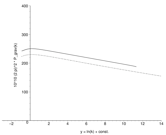
Figure 18: Power spectrum of tensor perturbations. The quantity plotted is $10^{10}(2\pi)^{2}\mathcal{P}_{\rm grav}(k)$ versus $y=\ln(k)+\mathrm{constant}$. The solid line is the numerical predictions. The dashed line is the best fit power law with exponential cutoff, offset by 20 units vertically for clarity. All parameters are described in the text.

Figure 18 shows the predicted tensor mode perturbation spectrum for our model (again with $\Omega_{0}=1.02$). Also shown (slightly offset) is the best fit model of the form of equation (65), together with an exponential cutoff at low $k$. This best fit is given by

$$10^{10}\,(2\pi)^{2}\,\mathcal{P}_{\rm grav}(k)=255(1-.023\,y)(1-\exp(-(y+2.6)/0.65))$$ (77)

valid again for $y>-0.93$. The slope in this formula is $255\times 0.023/(2\pi\times 10^{5})^{2}=1.48\times 10^{-11}$, which agrees well with the theoretical value of $32\mu^{2}/(3\pi)=1.47\times 10^{-11}$. If we form the ratio $r$ at $y=2$, which corresponds to $k=0.0016{\rm\,Mpc^{-1}}$ for $H_{0}=65\mathrm{\,km\,s^{-1}}{\rm\,Mpc^{-1}}$, we find $r\approx 0.19$. This is large enough to be detectable in the near future. For example, the predicted sensitivity level to B modes for the Planck satellite corresponds to a detection limit of $r>0.05$ [22], comfortably below the value predicted here. A relatively large tensor mode component is therefore a firm prediction of our model.

We end this section with a discussion of how to overcome the limitations of the slow-roll approximation and compute the primoridal power spectrum more accurately from first principles. The starting point for calculating the scalar curvature spectrum in a simple flat model is to write the linearised perturbed action in the form [23]

$$\delta_{2}S=\frac{1}{2}\int d\eta\,d^{3}x\left(v^{\prime 2}-\eta^{ij}v_{,i}v_{,j}+\frac{z^{\prime\prime}}{z}v^{2}\right),$$ (78)

where $v$ is a gauge-invariant combination of matter and metric perturbations, and $z$ is defined by $z=\phi_{0}^{\prime}/H$. Here $\phi_{0}$ is the unperturbed field, and the dashes denote derivative with respect to conformal time. By working in this way the entire problem is reduced to one of analysing a scalar field with a time-dependent mass term.

This approach generalises to the non-flat case, although here the definition of $z$ becomes more complicated [24]. Also, for closed models, the mode expansions necessary to carry out quantisation have to be performed using spatial sections given by the 3-sphere $S^{3}$. In this case the ‘comoving wavenumber’ $k$ takes on integer values, with $k=3$ its lowest (non-gauge) value. The mode equations found this way are very complicated, but retain the general form

$$v_{k}^{\prime\prime}+\left(k^{2}-f(\eta,k)\right)v_{k}=0.$$ (79)

In the flat case $f(\eta,k)$ would be $z^{\prime\prime}/z$, and in all cases $f(\eta,k)$ is calculable from knowledge of the background evolution.

The challenge now is to find suitable ‘quantum initial conditions’ so that after evolution through inflation, the variables $v_{k}$ can be used to find the perturbation spectrum. To achieve this involves a mode decomposition of $v_{k}$ into positive and negative frequency modes. The standard way to approach this is to assume that in the asymptotic past the background is either Minkowski or de Sitter, so that one knows the correct vacuum to chose. But this is clearly inappropriate here, as looking back in time we encounter the initial singularity.

The question of how to proceed in the absence of any asymptotic notion of the vacuum state has been widely discussed [13, 25, 26]. One simple approach is provided by Hamiltonian diagonalisation, where on each time slice modes are decomposed into positive and negative energy states by the Hamiltonian operator. But this technique tends to overestimate the particle production rate. A clear way to proceed was developed by Parker and Fulling [25, 26] and introduces the concept of an adiabatic vacuum. The application of this to the present case is complicated, but possible numerically, and initial results from this approach support a low-$k$ cutoff, although with effects less pronounced than we have found using the standard approximate techniques. This will be discussed in future work.

6 CMB power spectrum and large scale
structure

We now turn to using our primordial power spectra to compute the measured fluctuations in the CMB. For this purpose we use the CAMB package [27], which takes as its input the curvature spectrum and various cosmological parameters, and returns the $C_{\ell}$ values of the CMB power spectrum. For the cosmological parameters we take $\Omega_{\rm cdm}h^{2}=0.135$, $\Omega_{\rm b}h^{2}=0.0224$ and the optical depth to reionisation $\tau=0.17$. Together with $\Omega_{0}=1.02$ these correspond to the WMAP best fit values [1]. Additionally, we use a Hubble constant of $65\mathrm{\,km\,s^{-1}}{\rm\,Mpc^{-1}}$. This is lower than the best fit value quoted WMAP of $72\pm 5\mathrm{\,km\,s^{-1}}{\rm\,Mpc^{-1}}$. This latter value is obtained for an assumed flat model. If one relaxes the assumption of flatness, then the CMB data is quite degenerate with respect to the values of $H_{0}$ and $\Omega_{0}$ (see section 6.2 of Spergel et al. [1] for a discussion of this point). Our value of $H_{0}=65\mathrm{\,km\,s^{-1}}{\rm\,Mpc^{-1}}$ is compatible at $1\sigma$ with virtually all current determinations of $H_{0}$. For example, the HST Key Project value is $72\pm 8\mathrm{\,km\,s^{-1}}{\rm\,Mpc^{-1}}$ [28], whereas combined Sunyeav–Zel’dovich and X-ray flux measurements consistently favour a slightly lower value [29]. A lower value of $H_{0}$ was also suggested for closed models by Efstathiou [21], and our chosen value provides a reasonable fit with the WMAP power spectrum for $\Omega_{0}=1.02$. It is worth pointing out in this context that the WMAP simultaneous best fit values of $H_{0}$ and $\Omega_{0}$ actually provide a rather poor fit to their measured CMB spectrum!

In fixing $\Omega_{M}$ and $\Omega_{0}$ we in turn imply a value of $\Omega_{\Lambda}$. Together these pick out a unique path in the $\Omega_{M}$–$\Omega_{\Lambda}$ plane, for which we can calculate a total elapsed conformal time. In order to satisfy our boundary condition we need to achieve a value of conformal time by the end of inflation of $0.975$. The value of $b_{4}/\mu^{4/3}$ introduced in equation (54) was chosen to achieve this. With all the parameters now chosen, the computed CMB power spectrum is shown in figure 19. The fit is reasonably good, particularly at low $\ell$ where our model does show a fall off in power.

Figure 19: Predicted CMB power spectrum. These predictions are for a model with $\Omega_{0}=1.02$, as discussed in the text. The experimental points shown with $1\sigma$ error bars are the WMAP results.

Figure 20: The linear matter power spectrum. The solid line is the prediction from CAMB using as input our scalar primordial power spectrum. Long dashes are the 2dF measurements [30] convolved with the survey window function. The dot-dash line is a comparison fiducial model with $n_{s}=1$, $\sigma_{8}=1$, $h=0.7$, $\Omega_{m}h=0.2$, and $\Omega_{b}=0$.

A further test of our model is the predicted linear matter power spectrum. This is shown in figure 20, where it is compared with the 2dF data of Percival et al. [30]. Also plotted is a fiducial model with $n_{s}=1$, $\sigma_{8}=1$, $h=0.7$, $\Omega_{m}h=0.2$, and $\Omega_{b}=0$ (and therefore no baryon oscillations). This model is calculated from the fitting formulae of Eisenstein & Hu [31]. In order to achieve a good fit with the data, the vertical scale for our model predictions has been adjusted downwards by about 19%. Clearly, the model we have used so far needs some adjustment in its chosen parameters to correct the normalisation. But here we only we wish to compare the overall shapes of the three matter power spectra, leaving the overall normalisation aside. It is clear that the spectrum based on our non-power law primordial spectrum fits the 2dF data with a similar degree of fidelity to the power law-based fiducial model. On large scales (small $k$) both appear to overestimate the 2dF results. This can be explained by the fact that the 2dF results are given convolved with the survey window function, which has its largest effects at large scales (see figure 2 of Percival et al.). On smaller scales our results fit the shape of the 2dF spectrum very well. There is therefore no apparent problem in having a non-power law primordial spectrum right down to these scales. On even smaller scales the relevant comparison would be with Lyman-$\alpha$ data, but this area is still controversial and will not be discussed here.

So far we have developed a model based on the best fit WMAP values for $\Omega_{\rm cdm}h^{2}$, $\Omega_{\rm b}h^{2}$ and $\Omega_{0}=1.02$, but using a different value of $H_{0}$. This model does provide a reasonable fit, but figure 19 clearly leaves room for improvement, as does the normalisation of the matter spectrum. Ideally we would employ an MCMC analysis to find the best fit parameters for our model, but here we simply give an alternative model which improves the fit. This model has $\Omega_{0}=1.04$, so it still consistent with WMAP at the $1\sigma$ level. We also take $\Omega_{\rm b}h^{2}=0.0224$ (as before), $h=60$ and $\Omega_{\rm cdm}h^{2}=0.110$. Together these yield a value of $\Omega_{\rm cdm}=0.306$, which is reasonable. The values of $b_{0}$, $b_{4}$ and $\mu$ consistent with these are

$$b_{0}=2.3310,\qquad\frac{b_{4}}{\mu^{4/3}}=-0.2798,\qquad\mu=1.94\times 10^{-6}.$$ (80)

The lower value of $|b_{4}|$ produces a universe with larger curvature today. The results of this model are summarised in a best-fit curvature power spectrum given by

$$10^{5}\,2\pi\,\mathcal{P}_{{\mathcal{R}}}^{1/2}(k)=35.02(1-.023\,y)(1-\exp(-(y+0.20)/0.397)).$$ (81)

The result for the CMB power spectrum with these parameters is shown in figures 21 and 22. The former includes the WMAP points, and the latter plots both WMAP and the latest Very Small Array (VSA) data points, plotted on a linear scale [32]. This model clearly gives an extremely good fit to the observed spectrum, with the dip at low $\ell$ now quite pronounced. This is because an increase in $\Omega_{0}$ has the effect of sliding the graph to the right in $k$ space, as is clear from equation (59). There is also a good fit with the VSA data at higher $l$ values. The main disadvantage with this model is the low value of $H_{0}$, though this is still within $1.5\sigma$ of the HST Key Project value.

Figure 21: CMB power spectrum for a model with $\Omega_{0}=1.04$ (I). The parameters are discussed in the text. The experimental points shown with $1\sigma$ error bars are the WMAP results [1] and the dashed curve corresponds to the best fit $\Lambda$ CDM power law CMB power spectrum as distributed in the WMAP data products.

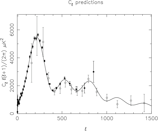
Figure 22: CMB power spectrum for a model with $\Omega_{0}=1.04$ (II). A similar plot to figure 21, but now plotted on a linear scale, with the latest Very Small Array data points also included to extend out to higher $l$ values (open circles).

7 Discussion

Many authors have argued that it is difficult to obtain realistic models of a closed inflationary universe [4, 5, 6, 7, 8]. One of the main problems is the low number of e-foldings required, which it is argued demand an unacceptable degree of fine tuning in the initial conditions for inflation. We have shown that this is not the case. It is relatively straightforward to construct inflationary models resulting in a universe which is measurably closed today, using only the simplest model of a free massive scalar field. These models have a number of attractive features and provide a very good fit to the observational data.

Motivated by the global geometry of de Sitter space, our model incorporates a quantisation condition on the available conformal time. This may seem uncomfortable from the point of view of causality, but it is quite sound from the viewpoint of wave mechanics. In field theory one regularly applies boundary conditions at temporal infinity, and the model presented here extends this idea to the universe. Furthermore, the constraint does not relate to the actual conformal time elapsed in the universe, but to the available conformal time at the point of creation of a homogeneous, idealised universe, before substantial structures have formed.

We hope that this quantisation condition will serve as a guide in constructing more detailed physical models of the processes taking place around the big bang, and that it might emerge from a quantum gravity understanding of this phase. Of course, many quantum gravity models of the very early universe involve tunneling from a Euclidean phase, in which case one cannot argue against the constraint on grounds of causality. Furthermore, for those who remain unhappy with our proposed constraint, we would point out that many of our conclusions do not depend crucially on it. One can relax the condition, explore the full space determined by the input parameters, and still make sensible predictions about the primordial power spectrum.

With a massive scalar field included, we find that initial data can be specified in terms of a pair of scale-invariant coefficients in the expansion of the scalar field around the initial singularity. These then determine the initial conditions for inflation. Quantum gravity effects will not be significant until well before the onset of inflation, so we are fully justified in running the evolution equations back to much closer to the initial singularity. Given only that we require of the order of 44 e-foldings we can conclude that the scale-invariant parameters $b_{0}$ and $b_{4}/\mu^{4/3}$ are both of order unity. Because we start close to the initial singularity, with infinite $H$, the model predicts a period of inflation in the early universe, independent of any question of generating super-horizon fluctuations. Furthermore, our condition on the total conformal time ensures that the matter-dominated plot in figure 6 represents the largest departure from flat that we can consider. The inflationary period drives us closer to flat and, assuming $\Omega_{M}\approx 0.3$ we are led to an $\Omega_{\Lambda}$ of around 0.7. Viewed in reverse, given input parameters $b_{0}$ and $b_{4}/\mu^{4/3}$ of order unity, together with our boundary condition, we predict an extremely small value for $\Lambda$, consistent with observation. The final parameter in the model is the mass ratio $\mu=m/m_{p}$, which is fixed by considering the growth of perturbations during the inflationary period.

The predictions of our model are robust against small variations of the input parameters. There is no question of the initial data being specified in a chaotic region of the classical dynamics. Chaotic behaviour in the inflationary equations in a closed universe was noticed by Page [33] and Cornish & Shellard [18]. But these authors considered initial data around $H=0$, whereas our parameters specify the fields as they exit the initial singularity, with $H=\infty$. The evolution therefore never enters the region of parameter space where chaotic evolution becomes relevant. The main element of fine tuning required in our model is setting $\mu=m/m_{p}$ to $\approx 10^{-6}$, but this type of tuning of the potential is a well-known feature of all inflationary theories [17]. Masses of the order of $10^{-6}m_{p}$ are quite legitimate from the viewpoint of high-energy physics, which we expect will shed light on the possible origins of such particles.

Our model makes a series of predictions. The universe is closed at around the level of a few percent, and we can explain the dip in the CMB power spectrum observed at low $\ell$. The statistical significance of this dip has been discussed by many authors [21, 34, 35, 36]. Their main conclusion is that this dip is not inconsistent with the spatially flat concordance model, but could still be an indicator of new physics, provided that any new model does not introduce too many additional parameters. In this respect our model is very efficient. Taking $\Omega_{M}$ and $\Omega_{\Lambda}$ as input data introduces two constraints on the three parameters $b_{0}$, $b_{4}$ and $\mu$. The one remaining degree of freedom is removed by fixing the scale of the overall perturbation amplitude. We also predict a running spectral index with reduced power at high-$\ell$ values. This looks to be favoured by dwarf galaxy and Lyman $\alpha$ data, though this area is controversial. The behaviour of the CMB spectrum beyond the second peak will also help break degeneracies in various models, and high-resolution measurements in this region would be extremely valuable.

For our best-fit models we typically predict of the order of 50 e-foldings. Such values are quite natural in our scheme, removing the central objection to closed universe cosmologies. Furthermore, a value of 50 has the additional feature of removing any potential problems with trans-Planckian physics [17]. That is, there is no question of Planck scale physics being inflated up to cosmological scales. A further indicator that our predictions are relatively insensitive to quantum corrections is provided by equation (40), which gives the value of the total energy in the universe as we leave the big bang. Assuming that $b_{4}/\mu^{4/3}$ is of order unity, this expression becomes

$$E_{\mbox{tot}}\approx\frac{0.03}{\mu^{2}}\frac{\hbar}{t}.$$ (82)

This tell us that the action $Et$ is very large, when measured in units of $\hbar$. This is reassuring, as it justifies treating the universe on the whole as a classical object. While quantum gravity effects will certainly alter how the universe behaves around the singular region, there is good reason to believe that the predictions of this paper will be largely unaffected by any such new physics. Furthermore, the limiting value of the action as $t\mapsto 0$ is large in units of $\hbar$, suggesting that the universe started in a highly improbable state. This will naturally favour spherically-symmetric initial conditions, and could also prove attractive from the viewpoint of the extremely low entropy that the universe has to have initially.

One further aspect of our model where considerations involving energy are relevant is the end of inflation, as the universe enters a reheating phase. Converting the energy density at the end of inflation into a temperature yields the reasonable value of $10^{16}$ GeV. This is as expected for typical reheating, if it occurs immediately after inflation is over. But as the scalar field exits inflation the universe is in a matter-dominated phase. Some process has to intervene which converts the scalar field into a radiation-dominated phase. Curiously, this may be difficult to achieve in a way which preserves the total, integrated energy, though there is little difficulty in demanding local conservation. This is probably a reminder that the ‘total energy’ in a closed universe remains a problematic concept in general relativity.

An important question is to identify the main experimental observations that will argue for or against our model. Our first key result is the low-$\ell$ dip in the power spectrum. The significance of this could be further enhanced by any lowering of the error bars in these measurements. While cosmic variance is the ultimate determining factor there is still some room for improvement, particularly in the question of foreground contamination [34]. The drop in the power spectrum at large $\ell$ is also a characteristic feature, which could be detectable with future observations. The third key prediction is the high value of $r$ — the ratio of tensor to scalar perturbations. This should also be observable by experiments such as the Planck satellite. It would also be of great interest to see which of these predictions is dependent on our choice of potential, and which survive if this restriction is removed.

We hope that much of the future work suggested by this paper is self evident. Before significant future work can begin we need to address the two main provisos mentioned in the text. The first is that mode quantisation in a closed universe has to be built in. The second is that the mode equations need to be integrated numerically, as aspects of the slow roll approximation are inadequate for our model. Neither of these pieces of work should prove too difficult, and a start has been made by Zhang and Sun [24] who appear to support our use of equation (61) as a leading order approximation. One area that we aim to address quickly is to explore in more detail the effects of varying the main input parameters, to explore the range of possible universes expected today. One significant point here is that all evolution is constrained to lie inside the matter curve of figure 6. This in itself is a significant restriction. In addition, the parameters chosen for the examples presented here were not computed by detailed model fitting. A full Bayesian determination of these parameters using all available data is clearly desirable, and will give a more stringent test of how well our model holds up.

Appendix A Conformal line elements

Here we establish spacetime conformal forms for the standard cosmological line elements for open, closed and flat cosmologies. (The fact that the Weyl tensor vanishes for cosmological models ensures that this is possible.) Our starting point is the FRW line element in the form

$$ds^{2}=dt^{2}-\frac{R(t)^{2}}{(1+kr^{2}/4)^{2}}\bigl{(}dr^{2}+r^{2}(d\theta^{2}+\sin^{2}(\theta)\,d\phi^{2})\bigr{)}.$$ (83)

This line element is already conformal in its spatial component. But a problem with this form is that $r$ is assumed to be dimensionless. To rectify this we introduce a constant distance $\lambda$ and replace the line element with

$$ds^{2}=dt^{2}-\frac{4\lambda^{2}R(t)^{2}}{(\lambda^{2}+kr^{2})^{2}}\bigl{(}dr^{2}+r^{2}(d\theta^{2}+\sin^{2}(\theta)\,d\phi^{2})\bigr{)}.$$ (84)

Here $t$, $r$, $\lambda$ and $R$ all have units of distance (assuming $c=1$). As usual, the constant $k$ is either $\pm 1$ or zero.

We seek a coordinate transformation to the spacetime-conformal line element

$$ds^{2}=\frac{1}{f^{2}}\bigl{(}d\mathsf{t}^{2}-d\mathsf{r}^{2}-\mathsf{r}^{2}(d\theta^{2}+\sin^{2}(\theta)\,d\phi^{2})\bigr{)},$$ (85)

where $f$ is a (dimensionless) function of $\mathsf{t}$ and $\mathsf{r}$. Clearly, from the angular terms, we must have

$$\frac{\mathsf{r}}{f}=\frac{2\lambda rR(t)}{\lambda^{2}+kr^{2}}.$$ (86)

In addition, the coordinate transformation must satisfy

$$d\mathsf{t} =f\cosh(u)\,dt+\frac{\mathsf{r}}{r}\sinh(u)\,dr$$

$$d\mathsf{r} =f\sinh(u)\,dt+\frac{\mathsf{r}}{r}\cosh(u)\,dr.$$ (87)

For flat cosmologies ($k=0$) we simply set $\mathsf{t}/\lambda$ equal to the conformal time $\eta$, with $\mathsf{r}=r$ and the hyperbolic angle $u$ set to zero. For non-flat cosmologies it is perhaps surprising to find that $u$ is non-zero. That is, there is a mismatch between the conformal coordinate frame and the cosmological frame.

The integrability conditions for the coordinate transformation provide a pair of differential equations for $u$:

$$r\frac{\partial u}{\partial r} =\sinh(u)$$ (88)

$$2\lambda rR(t)\frac{\partial u}{\partial t} =(\lambda^{2}+kr^{2})\cosh(u)+(-\lambda^{2}+kr^{2})$$ (89)

Equation (88) can be solved straightforwardly to give

$$e^{\mbox{\small$u$}}=\frac{1+rA(t)}{1-rA(t)}.$$ (90)

The function $A(t)$ is determined by equation (89), which reduces to

$$2\lambda R\dot{A}=\lambda^{2}A^{2}+k,$$ (91)

where the overdot denotes the derivative with respect to cosmic time $t$. The solution for $A$ depends on the curvature:

$$\lambda A=\begin{cases}\tan(\eta/2)&k=1\\ -\tanh(\eta/2)&k=-1.\end{cases}$$ (92)

The constant of integration has been chosen such that $A=0$ corresponds to $\eta=t=0$.

Next we solve the following pair of equations for $\mathsf{r}$:

$$r\frac{\partial\mathsf{r}}{\partial r}=\mathsf{r}\cosh(u),\qquad\frac{\partial\mathsf{r}}{\partial t}=f\sinh(u).$$ (93)

With a suitable choice of the arbitrary scale factor we find that

$$\mathsf{r}=\frac{\lambda^{2}A^{2}/k+1}{1-r^{2}A^{2}}\,r.$$ (94)

The remaining equations determining $\mathsf{t}$ are

$$r\frac{\partial\mathsf{t}}{\partial r}=\mathsf{r}\sinh(u),\qquad\frac{\partial\mathsf{t}}{\partial t}=f\cosh(u).$$ (95)

These are solved by

$$\mathsf{t}=\frac{\lambda^{2}+kr^{2}}{1-r^{2}A^{2}}\,\frac{A}{k}.$$ (96)

Here the arbitrary constant of integration has been fixed to ensure that $t=\eta=0$ corresponds to $\mathsf{t}=0$.

With $\mathsf{r}$ and $\mathsf{t}$ now found, we can write

$$f=\frac{\lambda^{2}A^{2}+k}{2\lambda AR}\mathsf{t}.$$ (97)

Our remaining task is to find an expression for $t$ in terms of $\mathsf{t}$ and $\mathsf{r}$. For this we use that result that

$$\frac{2\lambda\mathsf{t}}{\lambda^{2}+k(\mathsf{r}^{2}-\mathsf{t}^{2})}=\frac{2\lambda A}{k-\lambda^{2}A^{2}}.$$ (98)

The right-hand side is now a function of $t$ only, so the left-hand side can be used in place of cosmic time. Again, the explicit form depends on the cosmology. For spatially closed cosmologies we can write

$$\frac{2\lambda\mathsf{t}}{\lambda^{2}+\mathsf{r}^{2}-\mathsf{t}^{2}}=\tan(\eta)$$ (99)

whereas for spatially open we have

$$\frac{2\lambda\mathsf{t}}{\lambda^{2}+\mathsf{t}^{2}-\mathsf{r}^{2}}=\tanh(\eta).$$ (100)

The three cosmological scenarios can now be summarised as

$$f =\frac{\mathsf{t}}{R\sin(\eta)}=g\left(\frac{2\lambda\mathsf{t}}{\lambda^{2}+\mathsf{r}^{2}-\mathsf{t}^{2}}\right)\,\frac{\mathsf{t}}{\lambda}$$ closed

$$f =\frac{2\lambda}{R}$$ flat (101)

$$f =\frac{\mathsf{t}}{R\sinh(\eta)}=\bar{g}\left(\frac{2\lambda\mathsf{t}}{\lambda^{2}+\mathsf{t}^{2}-\mathsf{r}^{2}}\right)\,\frac{\mathsf{t}}{\lambda}$$ open

which are the results used in the main text.

References

- [1] D.N. Spergel et al. First year Wilkinson anisotropy probe (WMAP) observations: Determination of cosmological parameters. Astrophys. J. Suppl., 148:175, 2003.
- [2] D.A. Brannan, M.F. Espleen, and J.J. Gray. Geometry. Cambridge University Press, 1999.
- [3] C.J.L Doran and A.N. Lasenby. Geometric Algebra for Physicists. Cambridge University Press, 2003.
- [4] A. Linde. Can we have inflation with ? J. Cosmol. Astropart. Phys., 5:2, 2003.
- [5] A.A. Starobinsky. Spectrum of initial perturbations in open and closed universes. In M. Khlopov, M.E. Prokhorov, A.A. Starobinsky, and J. Tran Thanh Van, editors, Cosmoparticle Physics, page 43. Edition Frontiers, 1996.
- [6] J. Uzan, U. Kirchner, and G.F.R. Ellis. WMAP data and the curvature of space. MNRAS, 344:L65, 2003.
- [7] G.F.R. Ellis, W. Stoeger, P. McEwan, and P. Dunsby. Dynamics of inflationary universes with positive spatial curvature. Gen.Rel.Grav., 34:1445, 2002.
- [8] G.F.R. Ellis, P. McEwan, W. Stoeger, and P. Dunsby. Causality of inflationary universes with positive spatial curvature. Gen.Rel.Grav., 34:1461, 2002.
- [9] A.N. Lasenby and C. Doran. Conformal models of de Sitter space and initial conditions for inflation. To appear in proceedings ‘Phi in the Sky’, Porto, astro-ph/0411579, 2004.
- [10] A.N. Lasenby. Conformal geometry and the universe. Phil. Trans. R. Soc. Lond. A, to appear, 2003.
- [11] B. Ratra and P.J.E. Peebles. Inflation in an open universe. Phys. Rev. D, 52(4):1837–1894, 1995.
- [12] N.A. Chernikov and E.A. Tagirov. Quantum theory of scalar fields in de Sitter space-time. Ann. Inst. Henri Poincaré, 9A:109, 1968.
- [13] N.D. Birrell and P. C. W. Davies. Quantum Fields in Curved Space. Cambridge University Press, 1982.
- [14] B. Allen. Vacuum states in de Sitter space. Phys. Rev. D, 32:3136, 1985.
- [15] U.H. Danielsson. Inflation, holography, and the choice of vacuum in de Sitter space. J. High Energy Phys., 07:40, 2002.
- [16] W. Greiner. Relativistic Quantum Mechanics. Springer–Verlag, Berlin, 1990.
- [17] R.H. Brandenberger. Principles, progress and problems in inflationary cosmology. AAPPS Bull., 11:20, 2001.
- [18] N. Cornish and E.P.S. Shellard. Chaos in quantum cosmology. Phys. Rev. Lett., 81:3571, 1998.
- [19] A.R. Liddle and D.H. Lyth. Cosmological Inflation and Large-Scale Structure. Cambridge University Press, 2000.
- [20] J. Martin and D.J. Schwarz. The precision of slow-roll predictions for the CMBR anisotropies. Phys.Rev., D62:103520, 2000.
- [21] G. Efstathiou. Is the low CMB quadrupole a signature of spatial curvature? MNRAS, 343:L95, 2003.
- [22] G. Franco, P. Fosalba, and J.A. Tauber. Systematic effects in the measurement of polarization by the PLANCK telescope. Astron. Astrophys., 405:349, 2003.
- [23] V. F. Mukhanov, H. A. Feldman, and R. H. Brandenberger. Theory of cosmological perturbations. Phys. Rep., 215:203–333, 1992.
- [24] D. Zhang and C. Sun. The exact evolution equation of the curvature perturbation for closed universe. astro-ph/0310127, 2003.
- [25] L. Parker. Quantized fields and particle creation in expanding universes. I. Phys. Rev, 183:1057–1068, 1969.
- [26] S.A. Fulling. Aspects of Quantum Field Theory in Curved Space-Time. Cambridge University Press, 1989.
- [27] A.M. Lewis, A.D. Challinor, and A.N. Lasenby. Efficient computation of CMB anisotropies in closed FRW models. Ap. J., 538:473, 2000.
- [28] W.L. Freedman et al. Final results from the Hubble space telescope key project to measure the Hubble constant. Ap. J., 553:47, 2001.
- [29] M.E. Jones et al. from an orientation-unbiased sample of SZ and X-ray clusters. astro-ph/0103046, 2001.
- [30] W.J. Percival et al. The 2dF galaxy redshift survey: The power spectrum and the matter content of the universe. MNRAS, 327:1297, 2001.
- [31] D.J. Eisenstein and W. Hu. Baryonic features in the matter transfer function. Ap. J., 496:605, 1998.
- [32] C. Dickinson et al. High sensitivity measurements of the CMB power spectrum with the extended Very Small Array. astro-ph/0402498, 2004.
- [33] D.N. Page. A fractal set of perpetually bouncing universes. Class. Quant. Grav., 1:417, 1984.
- [34] G. Efstathiou. The statistical signficance of the low CMB multipoles. MNRAS, 346:L26, 2003.
- [35] G. Efstathiou. A maximum likelihood analysis of the low CMB multipoles from WMAP. MNRAS, 348:885, 2004.
- [36] C.R. Contaldi, M. Peloso, L. Kofman, and A. Linde. Suppressing the lower multipoles in the CMB anisotropies. JCAP, 07(002):1, 2003.