SZ polarisation as a probe of the intracluster medium

Abstract

We present high-resolution hydrodynamical simulations of the degree and direction of polarisation imprinted on the CMB by the Sunyaev-Zel’dovich effect in the the line of sight to massive galaxy clusters. We focus on two contributions to the electron rest-frame radiation quadrupole anisotropy in addition to the intrinsic CMB quadrupole that contributes most of the induced CMB polarisation: the radiation quadrupole seen by electrons due to their own velocity in the plane normal to the line of sight, and the radiation quadrupole due to the thermal Sunyaev-Zel’dovich effect, which is generated by a previous scattering elsewhere in the cores of the local and nearby clusters. We show that inside the virial radius of a massive cluster, this latter effect, although being second order in the optical depth, can reach the nK level of the former effect. These two effects can, respectively, constrain the projected tangential velocity and inner density profile of the gas, if they can be separated with multi-frequency observations. As the information on the direction and magnitude of the tangential velocity of the ICM gas is combined with the temperature Sunyaev-Zel’dovich effect probing the projected radial velocity it will be possible to improve our understanding of the dynamics of the ICM. In particular, future polarisation observations may be able to trace out the filamentary structure of the cooler and less dense ionized gas that has not yet been incorporated into massive clusters. We also discuss how the collapse of a cluster should produce a peculiar ring-like polarisation pattern which would open a new window to detect proto-clusters at high redshift.

1 Introduction

Recent measurements of the TE power spectrum of the intrinsic polarisation of the CMB by WMAP have put strong constraints on the total optical depth $\tau$ to the last scattering surface and on the possible nature of the sources responsible for reionisation. These measurements have also provided impetus for the further development of polarisation-sensitive receivers and for the theoretical modelling of the foregrounds contaminating the CMB polarisation.

On the other hand, new generation X-ray satellites such as Chandra or XMM-Newton have produced a wealth of high resolution maps of the intracluster medium (ICM) of nearby clusters. They support some aspects of our previous picture of the hydrostatic state of the plasma, but they invalidate others, and, most interestingly, bring out new phenomena such as cold fronts. However, it is well known that detailed studies of the cluster ICM in the X-ray band constrain the innermost parts, while the dynamics of the gas is also interesting at larger radii where for example gas flowing in from filaments, pristine gas accreting from the low-density regions of the Universe, or subclumps of cold gas of merging units encounter the hot ICM.

The Sunyaev-Zel’dovich effect (hereafter, SZ) encapsulates the processes of Thomson and inverse Compton scattering of CMB photons by the free electrons of the ICM (see, e.g. Sunyaev & Zeldovich 1980a; Carlstrom et al. 2002). In CMB temperature maps, both the thermal SZ (hereafter tSZ) effect and the kinetic SZ (hereafter kSZ) effects contribute to the secondary anisotropies. With CMB temperature variations depending at fixed observing frequency only on the gas pressure integrated along the line-of-sight, the tSZ effect has long been recognized as a powerful probe for studying the morphology of the ICM out to a substantial fraction of the virial radius of the cluster. The kSZ effect typically amounts to a few percent of the thermal effect and maps the bulk velocity of the ICM projected along the line of sight, to the extent that the ICM can be considered as a coherent bulk. Multi-frequency observations are necessary to separate the kSZ effect from the tSZ effect and extract information on the radial velocity of the gas. Recently, using Eulerian hydrodynamical simulations, Nagai & Kravtsov (2003) have studied the bias due to the internal motion of the gas in a massive, $2.4\times 10^{14}$$h^{-1}$ $M_{\odot}$ cluster on the estimates of the cluster bulk velocity along the same lines of sight where one measures the kSZ effect. While they focused on the ability to determine the global motions of massive haloes to later constrain cosmological parameters by means of the cluster pairwise peculiar velocities, it is also possible to constrain the motion of the ICM in the rest frame of the cluster. In fact, the kSZ effect and some of the SZ polarisation signals are complementary as they allow one to obtain information on, respectively, the projection along the line of sight of the density-weighted radial velocity of the gas, and the projection (amplitude and direction) along the line of sight of the density-weighted tangential velocity of the gas.

On CMB polarisation maps, the SZ-induced polarisation comes mainly from four terms. The first, which we want to emphasize, comes from single scattering of the quadrupole generated as radiation is Doppler–shifted due to the tangential motion of the gas (hereafter kpSZ), the second is due to single scattering of the CMB intrinsic quadrupole (hereafter ipCMB), and the last two are second scatterings of quadrupole anisotropies induced in the CMB by respectively previous t- and kSZ effects induced by first scatterings (hereafter respectively p²tSZ and p²kSZ ), when the y parameter/optical depth seen by the last scattering electron is not isotropic. These last two effects are potentially powerful probes of the central gas profiles in clusters.

For last scattering electrons inside and outside clusters, the p²kSZ effect is negligible relative to the p²tSZ effect if clusters are sufficiently hot and massive: these terms scale respectively as $\eta\tau^{2}$ and $\beta\tau^{2}$ (Sazonov & Sunyaev 1999, hereafter S99) where $\eta=kT/mc^{2}$ and $\beta$ the tangential velocity. Indeed, massive clusters have typically $\eta\simeq 3\;10^{-2}$ and $\beta\simeq 3\;10^{-3}$. While the ipCMB can reach levels of order 50 nK (S99), it is possible to eliminate it either by restricting oneself to local clusters at $z\mathrel{\hbox{\hbox to0.0pt{\hbox{\lower 4.0pt\hbox{$\sim$}}\hss}\hbox{$<$}}}0.3$ located in the directions of the z=0 CMB quadrupole where the ipCMB vanishes, or by using intensity maps of the tSZ effect and a model for the temperature distribution of the ICM. We will not tackle this term in detail as we consider that it is well understood and straightforward to simulate.

However, the relative amplitude of the ktSZ and the p²tSZ effects inside and in the vicinity of massive clusters calls for a more quantitative assessment as this is expected to depend strongly on the density and on the temperature profiles of the cluster. We will analyse the p²tSZ effect at some length, for three reasons. Firstly, the degree of CMB polarisation due to this second scattering of the tSZ has only been evaluated analytically, using spherically symmetric models for clusters (S99). Secondly, as pointed out by Sunyaev & Zeldovich (1980b, hereafter S80), it is interesting as the second scattering of the tSZ effect depends only on the local free electron density and not on the temperature, similarly to the scattering of the intrinsic CMB quadrupole. It can therefore be viewed as a means of detecting large–scale structures other than clusters: groups and filaments where the inner gas density is a few times the mean cosmic value. In this regime, its key advantage over the polarisation induced by the intrinsic CMB anisotropy resides in that it can be a factor of 10 more efficient, depending on observing frequency. Thirdly, and most importantly, double scattering can provide information about the inner gas density profiles of clusters, cross-checking the constraints derived from direct X-ray observations, which depend on a model for the local temperature of the gas when it is not possible to measure it directly.

Our hydrodynamical simulations show that maps of CMB polarisation can provide useful information about the profiles and dynamics of the ICM gas and constrain our picture of gas infall, mixture and heating as well as the dynamics of cold subclumps. They indicate a possible way to detect proto-clusters in their early stage of collapse. Besides, they show how the cluster SZ thermal effect can polarise the CMB over the filaments of gas between clusters.

The layout of this paper is as follows. In section 2, we review the analytical formulae we employ to compute the degree and direction of polarisation, due to kpSZ effect and to second scatterings of the tSZ effect, i.e. the p²tSZ effect. We present a semi-analytical description of the latter which enables us to obtain a substantial gain in computational time. We also summarise our assumptions. In section 3, we describe the setup of the simulations and the construction of the polarisation maps. Section 4 presents the strongest dependences of our results on the cluster gas profile. Section 5 discusses a general observational methodology to deal with contamination effects in order to retrieve the original projected density-weighted tangential and radial velocity field. Conclusions are presented in section 6.

2 Analytical description

In this section, we briefly summarise the analytical expressions we use for the main terms contributing to the polarisation of the CMB induced by the SZ effect discussed by S80 (see also S99, Chluba & Mannheim 2002).

We fix an orthonormal frame ($\overrightarrow{\bf X},\overrightarrow{\bf Y},\overrightarrow{\bf Z}$) at the point $P$ where the polarisation is induced: it is the position of the scattering electron in the case of single scattering, or the position of the last scattering electron in the case of double scattering. We choose the $\overrightarrow{\bf Z}$ direction along the line of sight, from $P$ to the observer. $\overrightarrow{\bf X}$ and $\overrightarrow{\bf Y}$ label the sky coordinates (we assume an euclidian patch). We use the Stokes parameters ($I$, $Q$, $U$, $V$) to describe the amount of polarisation as seen by an observer looking in a given direction. $I$ gives the total intensity of the light, while $Q$ and $U$ measure the degree of linear polarisation, and $V$ the degree of circular polarisation. Thomson scattering of anisotropic but unpolarised incoming radiation cannot generate circularly polarised radiation so that $V=0$. The degree of polarisation is given by:

$$p=\frac{\sqrt{Q^{2}+U^{2}}}{I},$$ (1)

and the direction of linear polarisation $\phi$, measured with respect to the $\overrightarrow{\bf X}$ axis, is:

$$\tan(2\phi)=\frac{U}{Q}.$$ (2)

In the rest of this section we deal with local effects on the line of sight. This approach is valid since the Stokes parameters are additive along the line of sight and the resulting $Q$ and $U$ seen by the observer read as follows:

$$\left\{\begin{array}[]{rcl}Q&=&\int~{}dQ\\ U&=&\int~{}dU,\end{array}\right.$$ (3)

where $dQ$ and $dU$ are local Stokes parameters at position ($\overrightarrow{\bf X},\overrightarrow{\bf Y},\overrightarrow{\bf Z}$). As we deal with small optical depths throughout the paper we assume that the background intensity $I_{0}$ of the CMB is not affected by SZ scattering: we set $I_{\mathrm{tot}}=I\simeq I_{0}$ to compute the degree of polarisation.

We now present in turn (1) the polarisation induced by the transverse motion of the gas with respect to the line of sight, (2) the effects of double scattering, and (3) the contribution due by scattering the CMB intrinsic quadrupole which together generate most of that part of the CMB polarisation due to the SZ effect. We will mention in the last paragraph of section 5 two other terms which can contribute a large fraction of the total polarisation of the CMB at a given frequency: the intrinsic polarisation imprinted at last scattering and the main types of foregrounds, i.e. dust grains and point sources emitting synchrotron radiation.

2.1 Kinetic polarisation

The kinetic polarisation kpSZ comes from single scattering of a CMB photon by a free electron moving in the plasma. Here, the electron rest frame anisotropy of the radiation necessary for Thomson scattering to generate polarisation is entirely due to the electron velocity (S80). We refer the reader to S99 and S80 for the detailed derivation and we just summarise their results here.

The $Q$ and $U$ components are given in the rest frame of the observer (all quantities depend on ($\overrightarrow{\bf X},\overrightarrow{\bf Y},\overrightarrow{\bf Z}$), though not explicitly written):

$$\begin{array}[]{rcl}dQ&=&-0.1I_{0\nu}\sigma_{T}f({x_{\nu}})n_{e}\beta_{t}^{2}\cos(2\chi)~{}d\overrightarrow{\bf Z}\\ dU&=&-0.1I_{0\nu}\sigma_{T}f({x_{\nu}})n_{e}\beta_{t}^{2}\sin(2\chi)~{}d\overrightarrow{\bf Z}\end{array}$$ (4)

Here, $\sigma_{T}$ is the Thomson cross-section, $n_{e}$ is the local density of electrons, ${x_{\nu}}$ is the dimensionless parameter of the Planck law: ${x_{\nu}}=\frac{h\nu}{kT}$, and:

$$f({x_{\nu}})=\frac{e^{{x_{\nu}}}(e^{{x_{\nu}}}+1)}{2\;(e^{{x_{\nu}}}-1)^{2}}{{x_{\nu}}}^{2}$$ (5)

is the spectral shape of the polarisation induced by the CMB in a non-relativistic approximation and simply is a translation of the black-body spectrum because of Thomson scattering, $\mu=\frac{\overrightarrow{v}\cdot\overrightarrow{\bf Z}}{|\overrightarrow{v}|}$, where $\overrightarrow{v}$ is the velocity of the electron and $\beta_{t}^{2}=\beta^{2}(1-\mu^{2})$ is its tangential component, and $\chi$ is the angle between the tangential velocity and the $\overrightarrow{\bf X}$-axis in the tangential plane. This effect is simple to implement as one simply needs to know the local state of the gas: given the value of each field everywhere in the simulation the summation is straightforward.

2.2 Double scattering due to finite optical depth

S80 noted that since the optical depth $\tau$ along the line-of-sight through massive clusters can reach $\sim 0.03$, double scattering cannot be neglected. In this case, CMB polarisation is due to second scattering of CMB secondary anisotropies generated by a first scattering in a dense region, either in the same structure or in a nearby one. The whole process can be alternatively viewed as scattering of the tSZ and kSZ effects. However, due to the kSZ effect being typically more than an order of magnitude smaller than the tSZ effect for massive clusters ( $\mathrel{\hbox{\hbox to0.0pt{\hbox{\lower 4.0pt\hbox{$\sim$}}\hss}\hbox{$>$}}}6\times 10^{14}$$M_{\odot}$), and as we will show that scattering of the tSZ (p²tSZ ) gives a degree of polarisation of the same order as the kpSZ effect of the previous paragraph, it is safe to neglect scattering of the kSZ (p²kSZ ). S99 give an explicit formal formulation of this second scattering effect:

$$\begin{array}[]{cl}dQ=&d\overrightarrow{\bf Z}\frac{3}{16\pi}\sigma_{T}n_{e}(\overrightarrow{\bf X},\overrightarrow{\bf Y},\overrightarrow{\bf Z})\\ &\times\int d\Omega~{}\sin^{2}(\theta)\cos(2\phi)\Delta I_{\nu}(\overrightarrow{\bf X},\overrightarrow{\bf Y},\overrightarrow{\bf Z},\theta,\phi)\\ dU=&d\overrightarrow{\bf Z}\frac{3}{16\pi}\sigma_{T}n_{e}(\overrightarrow{\bf X},\overrightarrow{\bf Y},\overrightarrow{\bf Z})\\ &\times\int d\Omega~{}\sin^{2}(\theta)\sin(2\phi)\Delta I_{\nu}(\overrightarrow{\bf X},\overrightarrow{\bf Y},\overrightarrow{\bf Z},\theta,\phi),\end{array}$$ (6)

where:

$$\Delta I_{\nu}(\overrightarrow{\bf X},\overrightarrow{\bf Y},\overrightarrow{\bf Z})=y_{\mathrm{eff}}(\overrightarrow{\bf X},\overrightarrow{\bf Y},\overrightarrow{\bf Z},\theta,\phi)f_{T}({x_{\nu}})I_{0\nu},$$ (7)

$$d\Omega=\sin(\theta)\,d\theta\,d\phi,$$ (8)

$f_{T}({x_{\nu}})$ is the frequency dependence of the tSZ effect:

$$f_{T}({x_{\nu}})={x_{\nu}}\frac{e^{x_{\nu}}}{e^{x_{\nu}}-1}\left({x_{\nu}}\frac{e^{x_{\nu}}+1}{e^{x_{\nu}}-1}-4\right),$$ (9)

and $I_{0\nu}$ is the intensity of the CMB at frequency $\nu$. $\theta$ and $\phi$ give the direction of the radiation incoming to the second scattering electron located at ($\overrightarrow{\bf X},\overrightarrow{\bf Y},\overrightarrow{\bf Z}$). With our axes, $\theta$ is the angle with respect to $\overrightarrow{\bf Z}$ (colatitude) while $\phi$ is the counterclockwise angle to $\overrightarrow{\bf X}$ in the ($\overrightarrow{\bf X}$,$\overrightarrow{\bf Y}$) plane. $y_{\mathrm{eff}}$ is the integral of $\eta\,d\tau$ as seen from ($\overrightarrow{\bf X},\overrightarrow{\bf Y},\overrightarrow{\bf Z}$) in the outward direction $(\theta,\phi)$ and is just the Compton y parameter in that direction. Interestingly, S80 pointed out that the degree of polarisation in double scattering at fixed tSZ effect “background” only depends on the local optical depth, and could be used to probe cooler regions than possible with temperature maps of the tSZ effect itself, provided of course that there is already sufficient sensitivity to measure the p²tSZ effect in the core regions of galaxy clusters.

In the following, we describe our computation in some length as we show that the p²tSZ effect depends sensitively on the detailed gas density profile of clusters, that it can in fact dominate in amplitude over the kpSZ effect and so should not be neglected in single frequency observations, and that it could also be of interest as a means of inducing large-scale polarised CMB radiation.

2.2.1 A spherical isothermal model for first scatterings

The double integrals in (6) are difficult to compute numerically: one needs to first evaluate from each point of the simulation volume an integral in all directions, and then to perform the summation along the line of sight. Therefore, we have adopted a semi-analytical model: we first choose a spherical, isothermal model for the clusters – here a $\beta$-model – to be able to compute $y_{eff}(\overrightarrow{\bf X},\overrightarrow{\bf Y},\overrightarrow{\bf Z},\theta,\phi)$ for each cluster. We define the $\beta$-model as:

$$\rho(r)=\rho^{*}\left[{1+\left(\frac{r}{r_{c}}\right)^{2}}\right]^{-3\beta/2}$$ (10)

(see, e.g., Komatsu & Seljak 2001) where $r_{c}$ is the core radius of the cluster and $\rho^{*}$ is a normalisation constant and we take $\beta=2/3$.

The important task is to estimate $\rho^{*}$ and $r_{c}$ for each cluster of the simulation. The optical depth as seen from $(\overrightarrow{\bf X},\overrightarrow{\bf Y},\overrightarrow{\bf Z})$ in the direction $(\theta,\phi)$ can be computed as:

$$\tau(\overrightarrow{\bf X},\overrightarrow{\bf Y},\overrightarrow{\bf Z},\theta,\phi)=\sigma_{T}\frac{1}{m_{p}\mu}\rho^{*}\int_{0}^{\infty}\frac{1}{1+\left(\frac{r(l)}{r_{c}}\right)^{2}}~{}dl\\ =\sigma_{T}\frac{1}{m_{p}\mu}\rho^{*}r_{c}^{2}\frac{1}{\sqrt{r_{c}^{2}+r_{0}^{2}-g^{2}(\overrightarrow{\bf X},\overrightarrow{\bf Y},\overrightarrow{\bf Z},\theta,\phi)}}\left(\frac{\pi}{2}\right.\\ \left.+\tan^{-1}\left(\frac{g(\overrightarrow{\bf X},\overrightarrow{\bf Y},\overrightarrow{\bf Z},\theta,\phi)}{\sqrt{r_{0}^{2}+r_{c}^{2}-g^{2}(\overrightarrow{\bf X},\overrightarrow{\bf Y},\overrightarrow{\bf Z},\theta,\phi)}}\right)\right),$$ (11)

where $l$ is the distance from the second scattering electron to the point taken along the line of sight $(\theta,\phi)$, $r_{0}$ is the distance between the point $(\overrightarrow{\bf X},\overrightarrow{\bf Y},\overrightarrow{\bf Z})$ and the cluster located at ($\overrightarrow{\bf X}_{c},\overrightarrow{\bf Y}_{c},\overrightarrow{\bf Z}_{c}$), $m_{p}\,\mu$ is the mean particle mass of the ICM, and:

$$g(\overrightarrow{\bf X},\overrightarrow{\bf Y},\overrightarrow{\bf Z},\theta,\phi)=(\overrightarrow{\bf X}-\overrightarrow{\bf X}_{c})\sin(\theta)\cos(\phi)+\\ (\overrightarrow{\bf Y}-\overrightarrow{\bf Y}_{c})\sin(\theta)\sin(\phi)+(\overrightarrow{\bf Z}-\overrightarrow{\bf Z}_{c})\cos(\theta).$$ (12)

$y_{\mathrm{eff}}(\overrightarrow{\bf X},\overrightarrow{\bf Y},\overrightarrow{\bf Z},\theta,\phi)$ is here the product of $\tau(\overrightarrow{\bf X},\overrightarrow{\bf Y},\overrightarrow{\bf Z},\theta,\phi)$ with the mean relative temperature $\eta=\frac{k_{\mathrm{B}}T_{e}}{m_{e}c^{2}}$, where $T_{e}$ is the mean temperature of the electrons, $m_{e}$ is the electron mass and $k_{\mathrm{B}}$ is Boltzmann’s constant. Once we have chosen the set of clusters which make the most contribution to the tSZ effect over most of the simulation, at each point $(\overrightarrow{\bf X},\overrightarrow{\bf Y},\overrightarrow{\bf Z})$ we can add up the local Stokes parameters obtained from (6) and (11) for each of these clusters to obtain the local $dQ$, $dU$ due to the p²tSZ effect.

The underlying assumptions here are first, the validity of the $\beta$-model for the radial profile of the gas, i.e. the validity of spherical symmetry and isothermality for the gas given that the X-ray surface brightness would be fitted by a $\beta$-profile, second, the validity of isothermality in the computation of the tSZ effect itself and third, the fact that lower mass groups and filaments will contribute very little to the tSZ effect as observed from any point of the simulation.

2.2.2 Estimating the core radius

Because we find the relative amplitude of the p²tSZ to the kpSZ effect to sensitively depend on the gas distribution, for massive clusters intersecting along the line of sight, we have computed the normalisation of the $\beta$-model in two ways. This ensures that we are not affected by resolution issues inherent to SPH such as gravitational softening. We first estimate the parameters numerically under the assumption that the cluster gas exactly follows a $\beta$-model, and we then derive an empirical best-fit to the actual simulated density profile of each cluster. This comparison also checks the validity of the $\beta$-profile for the simulated clusters.

Numerical approach

To estimate the free parameters $\rho^{*}$ and $r_{c}$ numerically, we first identify clusters using a friends-of-friends groupfinder (Davis et al. 1985) with linking length 0.2 times the mean interparticle separation. We then compute the virial mass and radius $m_{\mathrm{vir}}$ and $r_{\mathrm{vir}}$ starting from the most bound gas particle of the cluster. Note that we use only gas particles to estimate $m_{\mathrm{vir}}$ and $r_{\mathrm{vir}}$. We define the virial radius as the point where the enclosed gas density falls to $\Delta_{c}\,\rho_{c}\,f_{\mathrm{bar}}$ where $\Delta_{c}$ is the virialization overdensity (Bryan & Norman 1998), $\rho_{c}$ is the critical density of the universe and $f_{\mathrm{bar}}=0.13$ is the mean cosmological gas fraction. We suppose that the cluster only extends up to the virial radius. Starting with an analytical expression for the virial mass $m_{\mathrm{vir}}$ as a function of $\rho^{*}$ and $r_{c}$, it is possible to express the mass inside the core radius $m_{c}(r_{c})$ as a function of $m_{\mathrm{vir}}$ and $r_{c}$. At fixed $m_{\mathrm{vir}}$, we then iterate to find the core radius: it is obtained by choosing a test radius $r_{t}$, computing the mass $m(<r_{t})$ inside $r_{t}$ and comparing it to $m_{c}(r_{t})$. Practically, we start from the most bound particle of the cluster and increase $r_{t}$, up to the desired core radius where $m(r_{t})=m_{c}(r_{t})$ where we then set $r_{c}=r_{t}$.

Best-fit approach

As a second approach, we directly fit the $\beta$-model to the gas density profile measured in the simulation. We employ an adaptive number of points depending on the number of particles in the cluster so that noise fluctuations on small haloes can be reduced. We always take more than 300 particles per halo to give a good fit, with the number of fitting points less than 100, and we limit ourselves again to the virial radius. We find reasonable agreement between the two approaches, showing that the $\beta$-profile and spherical symmetry are fair assumptions. When computing the p²tSZ effect in the simulations, we employ the second approach which gives fast results and depends on both the inner and outer parts of the cluster. For the massive cluster that we find in our high resolution simulation we compute $\mbox{$m_{\mathrm{vir}}$}=1.5\times 10^{15}\mbox{$M_{\odot}$}$ and the numerical and best-fit approaches give respectively $r_{c}=250$ kpc and $370$ kpc.

2.2.3 Semi-analytical results

Having set the gas density profile for the integration of (11) over the path of the incident radiation on the second scattering photon, we proceed to integrate  (6) over $(\theta,\phi)$ numerically. Figure 1 shows the results of the computation of $Q$ and $U$, for a spherically symmetric gas distribution following a $\beta$-profile with core radius $150$ kpc. Here and in all subsequent figures we take $x_{\nu}=3$: we discuss the frequency dependence of the effects in section 4.

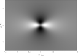
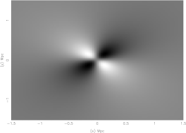
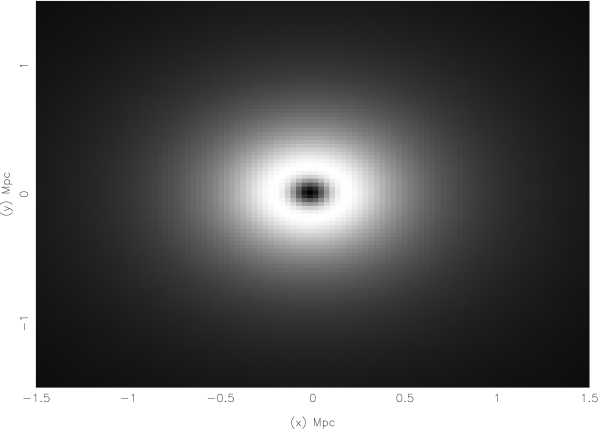
Figure 1: The top images gives the value of $Q$ and $U$ (left and right panels respectively) of the polarisation of the CMB due to second scattering of the in-situ tSZ effect for a 150 kpc core radius cluster put at the centre. The figure illustrates the spatial variations of $U$ and $Q$ but the real level of polarisation will include an overall factor dependent on the normalisation of the matter density profile. The gray scale is linear in $Q$, $U$ and the polarisation. Black is for the minimum relative value and white for the maximum relative value. The change in the intensity of the polarisation is clear at the centre. As expected the axis of $Q$ and $U$ are rotated by $\pi/4$ and the axis of $Q$ is orthogonal to the $x$-axis. The global degree of the polarisation, as given by $\sqrt{Q^{2}+U^{2}}$ for $I=1$, is shown in the lower image. Note the annulus of high intensity around the core and the fall-off at the centre as spherical symmetry washes out the signal.

As expected, the polarisation has circular symmetry. The signal vanishes at the centre of the cluster because of the particular symmetry involved at that point: the centre of the cluster does not see any changes due to any rotations of the space around it, so that there can be no polarisation induced at this point. As a consequence, the intensity pattern shows an annulus: we checked that the radial distance $r_{\mathrm{max}}$ to the circle on the annulus where the degree of p²tSZ is maximum scales as $r_{\mathrm{max}}=1.3\,r_{c}$. Note that this feature has already been found by S99 (see their figure 3) who also integrate their equations numerically: their King profile with n=1 is similar to the $\beta$-profile assumed here.

2.3 Polarisation due to the CMB quadrupole

Thomson scattering of the intrinsic quadrupole of the CMB by the free electrons of the ICM will contribute to the degree of polarisation observed toward massive clusters. S99 show that this term can reach $2\times 10^{-6}\;\tau\;\sim\;4\times 10^{-8}$ for $\tau=1/50$, comparable and even higher than the polarisation due to the kpSZ or p²tSZ effects presented above. However, at low redshift, there are four orthogonal directions in the sky where one expects the degree of CMB polarisation due to the scattering of the quadrupole component to vanish (see Fig.1 of S99). In practice, the directions towards which the CMB quadrupole vanishes have been determined with some accuracy by WMAP: one is near $(l,b)\simeq(-80\degr,60\degr)$, a direction close to the Virgo cluster (Tegmark et al. 2003). Note that this only holds for local clusters ($z\mathrel{\hbox{\hbox to0.0pt{\hbox{\lower 4.0pt\hbox{$\sim$}}\hss}\hbox{$<$}}}0.3$), as objects at higher redshift will observe a different realisation of the primordial quadrupole (Kamionkowski & Loeb 1997).

3 Rendering a galaxy cluster

3.1 Parameters and setup

We use the public version of gadget (Springel et al. 2001) to run the simulations after modifications to include the “standard entropy” formulation (Springel & Hernquist 2002), cooling of the gas and photoionisation by a uniform UV background. The simulations follow a cube of $70$ Mpc comoving side and assume a concordance $\Lambda$CDM cosmology with $\Omega_{0}=0.3$, $\Omega_{b}\>h^{2}=0.019$, $\Lambda=0.7$, $h=0.7$. We have not switched on cooling and photoionisation in this study but we will analyse their impact in a forthcoming paper ; here the evolution is fully adiabatic which suffices for our purpose.

We constrain the density field using the implementation of the Hoffman-Ribak algorithm proposed by van de Weygaert & Bertschinger (1996) to obtain a massive cluster at the end the simulation. To obtain a cluster of approximately $1.5\times 10^{15}$$M_{\odot}$ we constrain the initial conditions to have a gaussian peak with $\sigma=13.5$ Mpc in the centre of the box. The height of the peak is three times the rms value obtained by smoothing an unconstrained density field with the same gaussian kernel. At z=0, the optical depth of the central region of the cluster is $\sim 3\;10^{-2}$ and the mean electron temperature in the virialised gas is $\sim 15$ keV: the cluster is more massive than Coma, and probably closer in mass to Perseus.

To speed up the simulation we have used mesh refinement when constructing the initial conditions: after running a low resolution simulation the particles of the cluster have been traced back to the initial redshift to find the Lagrangian region containing all the mass virialised by z=0. We have used two simulations: in the first the initial density field is realised on a $64^{3}$ mesh embedded in a $32^{3}$ mesh covering the whole volume, while the second uses a $128^{3}$ mesh embedded in a $64^{3}$ mesh. In the two simulations, we have used the same phases for the common density perturbation modes so as to verify the stability of the method with respect to mesh resolution. We put high mass DM and gas particles on the nodes of the low-resolution grid and low mass DM and gas particles on the nodes of the high resolution grid. Following common practice, we set the softening length of both low and high resolution particles (we use the subscripts “lr” and “hr” in the following) to one tenth of the their mean interparticle separation. The softening length $l_{\mathrm{soft}}$ is kept fixed in comoving coordinates: $l_{\mathrm{soft,lr}}=400\mbox{kpc}$ and $l_{\mathrm{soft,hr}}=30\mbox{kpc.}$ We have checked that the overall intensity of the effects and the gas distribution is the same within a factor of two between the simulations, and in the rest of the paper we will only discuss the simulation with high mesh resolution.

The z=0 map of the density projected along the $\overrightarrow{\bf Z}$ direction of the whole box is shown in Figure 2. The box is 70 Mpc wide. The friends-of-friends groupfinder finds a little more than $3.5\times 10^{5}$ DM particles in the central cluster, while there are $N_{\mathrm{lr}}=171019$ and $N_{\mathrm{hr}}=729000$ DM particles in total, with masses $M_{\mathrm{lr,DM}}=2.61\times 10^{11}$$M_{\odot}$ and $M_{\mathrm{hr,DM}}=3.26\times 10^{10}$$M_{\odot}$ and the same number of gas particles with masses $M_{\mathrm{lr,gas}}=3.93\times 10^{10}$$M_{\odot}$ and $M_{\mathrm{hr,gas}}=4.92\times 10^{9}$$M_{\odot}$.

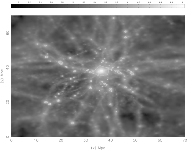
Figure 2: Map of the gas density of the whole high resolution simulation projected along the line of sight. The side is $70$ Mpc and the cluster is located close to the middle of the box (as it is along the line of sight). There are four filaments reaching the cluster and extending at close to right angles. The colour scale is in decimal logarithm of arbitrary units in projected density.

3.2 Mapping the SZ effect

To render the SZ effect we have built a parallel imager capable of integrating any physical quantity along the line of sight in the simulation. The imager includes the sph kernel of gadget and tree neighbour searching so that physical quantities are well computed at each 3D pixel of the simulation volume. The tree is filled with the sph particles and we use this to compute the local physical effects with the same algorithm that is used to estimate hydrodynamical forces on a particle. We then integrate up the results along the line of sight (here the $\overrightarrow{\bf Z}$ direction). Figures 3 and 4 show the p²tSZ effect and the kpSZ effect respectively. The figures show a box 70 Mpc wide and we have projected the full thickness of the simulation. Furthermore, to compare with the distribution of the projected gas velocities we plot these in Figure 5, where we have projected only the gas velocities and gas densities from a 3 Mpc thick slice containing the highest density region of the simulation i.e. the centre of the cluster (the width is again 70 Mpc). We select isodensity levels in Figure 2 and show them on the other figures to make a comparison between the polarisation signal and the possible presence of clumps of dense gas. The colour scales for the polarisation plots have been kept the same to facilitate the comparison. Following Nagai & Kravtsov (2003) we have tested the effect of convolving the resulting maps with a gaussian kernel corresponding to $1$ arcminute FWHM. Putting the cluster at z=0.1 this would represent a physical scale of 77.5 $h^{-1}$ kpc. In practice, we find that convolution leaves the large scale features of the maps unchanged but removes some details in the zoomed map of the kSZ effect shown in Fig. 6 which has a 20 Mpc width. As a result, we present all maps but that of Fig. 6 unconvolved for simplicity.

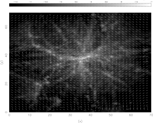
Figure 3: Map of the p²tSZ effect for the main cluster of the highest resolution simulation. The figure shows a box $70$ Mpc wide and the whole box has been projected. The decimal logarithm of the degree of polarisation is colour-coded with the scale provided at the top. This scale has been frozen to facilitate the comparison with the other maps. Radial lines coming from the central cluster are an artifact of the limited number of steps for the integration on $\phi$ in equation (6); they could be avoided but at the expense of unreasonable computing time, the CPU scaling as the number of iterations. Note the fall-off of the p²tSZ effect as one approaches the centre of the cluster: increasing symmetry tends to wash out the signal. Note also the residual polarisation on the filament leaving to the east: this shows the possibility of the p²tSZ effect tracing large-scale structure.

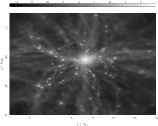
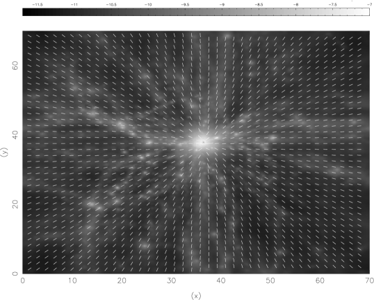
Figure 4: Maps of the kpSZ effect in the highest resolution simulation. The figure shows a box $70$ Mpc wide and the whole box has been projected. The decimal logarithm of the degree of polarisation is colour-coded with the scale provided at the top (it is the same scale as in Fig. 3). It has been computed using equation (4). Contours of the projected gas density have been added to the top image to make a precise comparison with previous maps. The directions of polarisation due to the kpSZ effect are shown on the bottom image.

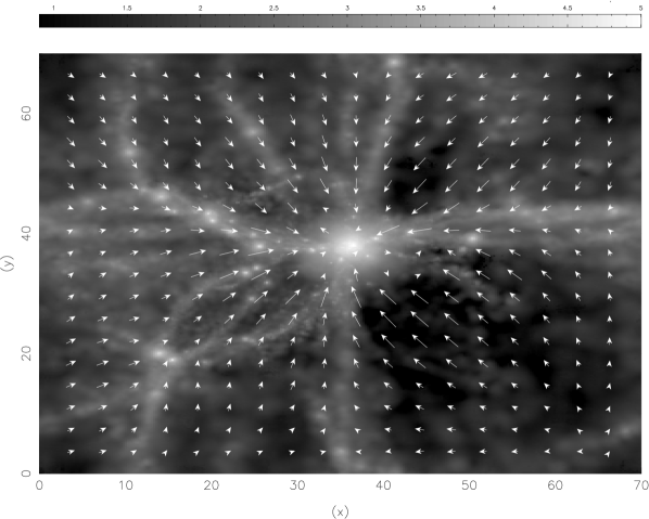
Figure 5: Maps of the projected density and of the projected gas velocity field in the highest density slice of the simulation. The width is 70 Mpc and the thickness 3 Mpc. The length of the arrows is proportional to the velocity with a maximum of approximately $2000$ km s^-1 .

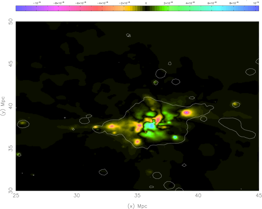
Figure 6: Map of the kSZ effect in terms of $\Delta T/T_{CMB}$. The change in temperature is shown with a colour linear between $\simeq-10^{-5}$ and $\simeq 10^{-5}$. Density contours have also been overplotted on the map but please note that it is now only $20\;\mbox{Mpc}$ wide. Small scale details have been smoothed out as we have the convolved the image with a Gaussian beam of FWHM 1’

4 Dependence on physical parameters

In this section, we first discuss features of the p²tSZ effect associated with resolution issues in the core of the cluster. Then we compare the p²tSZ effect to the kpSZ effect. The location and intensity of the bright annulus of the p²tSZ effect can provide useful cross-checking information on X-ray observations and in particular on the validity of the $\beta$-profile as an accurate description of the projected inner density of the gas, while the kpSZ effect can constrain the projected density-weighted tangential velocity of the gas.

4.1 Dependence of the p²tSZ effect on cluster internal gas profile

4.1.1 Effect of the internal structure on the intensity of the p²tSZ effect

As we have pointed out above, the computation of the polarisation due to double scattering involves two integrals. The first one integrates the effect along the line of sight while the other calculates the anisotropy of the incoming radiation at each point of the line of sight. In regions of high electron density, the two consecutive scatterings will happen at almost the same location and we should therefore expect the polarisation term due to double scattering to contain a strong dependence on the spatial distribution of electrons in the cluster. In fact, if we calculate the Stokes parameters for a toy model (here a $\beta$-model for the gas density profile), we find that the overall signal will scale as $n_{0}^{2}r_{\mathrm{c}}^{4}$. From this example we infer that the double scattering term will be very sensitive to the internal gas structure of the cluster like the inner radial density slope or the possible presence of a core which will affect both $r_{\mathrm{c}}$ and $n_{\mathrm{0}}$. If the angular resolution is sufficient, the p²tSZ effect could detect clumps of dense cold gas orbiting in the ICM such as remnants of minor mergers or even cold fronts provided their density contrast with respect to the surrounding hot ICM is high enough.

We have already noted in paragraph 2.2.3 that the two scattering terms will show a very particular polarisation pattern with an annulus around the centre of the cluster, and that the radius $r_{\mathrm{max}}$ of the maximum of intensity of this annulus is simply related to the core radius if one assumes a $\beta$-profile.

4.1.2 Effect of resolution on the estimation of the core radius

As pointed out above, the maximum degree of polarisation $p_{\mathrm{max}}$ of the radiation after the second scattering of the thermal effect depends significantly on the core radius of the $\beta$-profile of the gas. Consequently, $p_{\mathrm{max}}$ may easily vary by a factor 2 for reasonable values of $r_{\mathrm{c}}/\mbox{$r_{\mathrm{vir}}$}$. This can be advantageous in the case of multi-frequency observations, where one can separate the kpSZ from the p²tSZ effect and use only the latter to constrain the gas density in the central region. On the other hand, it shows that it will be difficult to disentangle both effects when only a single frequency is available. In any case, it is essential to have a robust estimate of the order of magnitude of the intensity of the polarisation signal which is not plagued by resolution issues. In all the above, we have ignored the central softened part of the cluster as we computed the core radius of the gas according to the $\beta$-model because it introduces artificial smoothness in the derived cluster gas profile. We have noticed that when we skip the inner region as one would do to suppress the dependence on the resolution of the simulations, the order of magnitude of the p²tSZ effect can significantly increase if one uses the “numerical approach” of 2.2.2 to estimate it. However, the cluster gas profile parameters $r_{\mathrm{c}}$ and $\rho_{*}$ obtained in this case with the numerical approach are reasonably close to those resulting from best fitting a $\beta$-model, showing that the amplitude we derive for the p²tSZ effect inside massive clusters is robust in this case.

To summarise, even if a very precise computation of the intensity of the p²tSZ inside clusters will require accurate knowledge of the gas profile, our simulations conversely prove that, once it is singled out in observations, it can prove a powerful tool for constraining the gas profile.

4.2 Comparison of the two intensities

We have confirmed numerically the analytical predictions of S80 and S99 that finite optical depth effects are not negligible and that second scattering of the thermal SZ effect may be the dominant source of SZ polarisation other than the intrinsic CMB quadrupole in the case where the optical depth is high enough. In this paragraph, we compare the intensities of the p²tSZ and the kpSZ effects first with respect to their spatial distribution in the cluster, then with respect to the observing frequency. We also discuss the directions of polarisation of the p²tSZ and the kpSZ effects.

4.2.1 Spatial variation

The peak of the kpSZ effect is located near the centres of gas clumps or close to the centres of clusters but seldom directly on them. As the kinetic polarisation reflects mostly the part of the tangential velocity of the gas which is coherent over some scale this is not unexpected because the gas inside discrete clumps or in the core region of the cluster may have thermal velocities largely in excess of the bulk motions while gas accretion on these structures can reach bulk velocities of order of $1000\;\mbox{km s${}^{-1}$}$ which does more than compensate for the difference in projected density.

When the accreting gas reaches the local density maxima its velocity distribution becomes isotropic, hence reducing the signal. This is the case, for instance, for the infall one can observe just under the central cluster (in green), at $x\sim 35$ Mpc and $y\sim 35$ Mpc in the bottom map of Fig. 4: it is associated neither with a local peak of density nor with the virial radius of the cluster. It is plain gas accretion, in other words, a coherent inflow. On the opposite side of the cluster, a clump above the central regions (clearly seen in Fig. 2 at $x\sim 45$ and $y\sim 55$ Mpc) is almost absent from the kSZ map. If the gas density profile in the very central region of a halo is sufficiently symmetric, any similar steep variation in the tangential velocity of the gas (accretion or outflow because of AGN or SN feedback) would lead to possible detection of the inner ring in the kpSZ maps. Farther out, dense cold fronts resulting from recent mergers could also make a strong signature in kpSZ maps, as they are thought to be contact interfaces separating the hot gas of the ICM and the cold gas of the subclumps as the two phases move with transsonic velocity with respect to each other.

It may be noticed that the intensity map for the kpSZ effect is sharper than for the p²tSZ effect. This is mainly because the polarisation follows the locations where the gas accretes on the high density regions or reaches high velocities, and because changes in the projected velocity field of the ICM can be very abrupt and combine with variations of the projected gas density. On the other hand, the p²tSZ effect mostly follows the projected density and temperature with the latter being much smoother than the variation of velocities.

4.2.2 Frequency variation

The different frequency-dependence of the p²tSZ and kpSZ effects will introduce changes in the degree and direction of polarisation of the resulting combined signal as the observing frequency changes.

As an example, we briefly discuss the effects expected as the observation frequency changes from ${x_{\nu}}<3.83$ to ${x_{\nu}}>3.83$, looking at infalling gas on the outskirts ($r\mathrel{\hbox{\hbox to0.0pt{\hbox{\lower 4.0pt\hbox{$\sim$}}\hss}\hbox{$<$}}}r_{\mathrm{vir}}$) of a massive cluster.

For ${x_{\nu}}<3.83$ the direction of polarisation of the p²tSZ effect is approximately orthogonal to the direction of the kpSZ effect. As the cluster is the geometrical centre for both the accretion and the tSZ effect, it can be viewed as a point source far from the core. Therefore both effects share the same symmetry but one is rotated $90\degr$ with respect to the other. Because they have similar intensities they may counterbalance one another and the resulting degree of polarisation can vanish. Conversely, if ${x_{\nu}}>3.83$ the two effects are coherent and oriented in the same way so they will amplify: the signal can be twice as large. (Recall that in all our figures we have assumed an $x_{\nu}=3$.)

4.2.3 On the direction of the resulting polarisation

The direction of polarisation of the kpSZ effect is clearly orthogonal to the direction of the tangential velocity of the gas. In our simulations the cluster is massive enough to drag the gas from even the distant edges of the box: on the velocity fields, arrows in the outskirts of the box are pointing towards the central cluster. It is interesting to note that along major structures like filaments this favoured orientation is also significantly enhanced: coherent motion of the gas is amplified over such regions. Conversely, at this level of resolution, the orientation of polarisation may point toward a completely arbitrary direction over the close outskirts of the cluster: the signal generated by gas accretion can interfere with that due to the presence of slowly moving, high density clumps around the cluster.

5 Observational prospects

In this section, we go beyond using SZ polarisation to constrain only the dynamics and density profile of the ICM. We first discuss how the detection of the kpSZ polarisation could be used as a tracer of collapsing objects. Then, we present the p²tSZ effect as a means of probing external structures. Finally, we discuss the contaminating polarisation induced by other dominant SZ effects, by the CMB polarisation, by dust, and by the cluster magnetic field.

5.1 The kinetic polarisation term as a probe of collapsing structures

The key feature of the polarisation due to the kinetic term is its dependence on the tangential component of the velocity. In the situation where a structure is collapsing under the effect of its own gravity, the velocity vectors point toward the centre of the structure. In this situation it is possible to calculate the integrated effect along the line of sight at the angular direction $\theta$ from the centre. The degree of polarisation scales as:

$$\mathrm{p}\propto\int n_{e}(v\cos(\alpha))^{2}dl$$ (13)

where $v\cos(\alpha)$ gives the tangential component of the velocity vector. We can substitute $\cos^{2}(\alpha)=d^{2}/(d^{2}+l^{2})$ where $d=\theta D_{\mathrm{ang}}$ with $D_{\mathrm{ang}}$ the angular diameter distance to the cluster. This integral over the line of sight of the tangential component times electron density will reach a maximum at some point between the centre of the structure and its radius but this maximum will never happen at the centre of the structure since in this case the tangential component of the velocity is very small ($\cos(\alpha)\rightarrow 0$).

Figure 7: The solid line shows the polarisation due to the collapse of a cluster ($r_{c}=150$ kpc and $n_{e}=10^{-3}\mbox{gr/cm${}^{3}$}$) with a homogeneous collapsing velocity of 800 km/s. The dotted line shows the effect due to the bulk motion of the cluster with respect to the Hubble flow for a tangential velocity of 300 km/s. The real polarisation amplitude is the product of the plot times the corresponding frequency dependence.

Although the above discussion was focused on a cluster, the same discussion will be valid for a structure which is still collapsing, such as proto-clusters. This opens the exciting possibility of detecting the clusters even before their collapse time. This is because the collapse polarisation term is proportional to the collapse velocity squared times the optical depth which is the same for a cluster already formed and for its progenitor in the collapsing process, and also because temperature does not play any role. In fact, we only require that the gas cloud is ionised and collapsing. It could be possible to see this gas in SZ polarisation forming a ring around the centre of the cloud before it starts to emit X-rays or before its temperature is high enough to create a substantial thermal SZ effect. At distances $r>r_{c}$, the collapsing term will dominate the effect due to the bulk motion of the cluster. This comes from the higher collapsing velocities expected for a typical cluster when compared with its expected bulk motion. An example is shown in Fig. 7, where the shape of the kpSZ effect expected for a spherical proto-cluster collapsing with a homogeneous collapsing velocity of 800 km/s (solid line) is compared to the effect of bulk motion of the cluster assuming a tangential peculiar velocity of 300 km/s (dotted line).

5.2 The finite optical depth effect as a polarisation generator

S80 have noted that CMB polarisation due to double scattering effects can bring out gas structures much less overdense than the virialised regions of massive clusters: smaller groups and filaments with sufficient optical depth may become sources of polarised sub-mm radiation, although to a very small degree. This is because the second scattering of the primary CMB modified by either the tSZ or the kSZ effect does not depend on the local temperature or on the local velocity, but only on the local optical depth. As a result, if it is possible to measure the few nK of the p²tSZ effect up to the outskirts (e.g., $r_{\mathrm{vir}}$) of massive clusters, it will be feasible to detect filaments as clusters would provide the tSZ input to generate the additional CMB anisotropy. An example of this effect is the left filament leaving the cluster in the NW direction in Fig. 3 (see at $x\sim 20$ Mpc and $y\sim 40$ Mpc), which is less apparent in the kpSZ map (Fig. 4). This is in contrast to the mapping potential of the tSZ effect in temperature which is essentially restricted to lines of sight where the integrated Compton parameter $y$ reaches substantial values because at each point, the high local temperature must contribute to significant pressure.

To summarize, it is possible to detect filaments, first, by mapping an area of the sky and second, by modelling the distribution of nearby clusters: it may be possible to predict the direction of polarisation expected on a given region of the filament. Here, simulations including photoionisation from the UV background that strongly affects the IGM are necessary to make a quantitative assessment.

5.3 Contamination effects

The kpSZ and p²tSZ effects are probes that follow respectively the dynamics and the inner density profile of the ICM but it is not clear whether they may be detectable in the near future. Intrinsic CMB polarisation, SZ effects (scattering of the intrinsic quadrupole, and possibly even octupole: Challinor et al. 2000), the tangential kinetic effect, and second scattering of the tSZ and kSZ effects), foregrounds such as Galactic dust and Galactic synchrotron emission or radio point sources with synchrotron emission all contribute to the polarisation of the incoming sub-mm signal. These effects have a different frequency dependence except for scattering of the CMB intrinsic quadrupole which depends linearly on ${x_{\nu}}$ in the same way as does second scattering of the kSZ effect. The obvious way to separate components will be with multi-frequency observations.

However, the situation could be tractable even at a single frequency, provided one obtains an image with sufficiently high resolution to avoid point sources. Galactic dust and Galactic synchrotron emission induce a high degree of polarisation, but dust maps will enable one to correct for some of the contamination or at least to set a lower galactic latitude for the observations. Magnetic fields in the Galactic ISM will Faraday rotate the plane of polarisation, however, Faraday rotation depends strongly on the frequency. Because our present knowledge of the Galactic magnetic field is still crude this constraint may also translate into a minimum Galactic latitude for observations or to a lower bound for the operating frequency.

Removal of the intrinsic CMB polarisation is feasible, as their fluctuations are typically on scales larger than the ones considered here (i.e. greater than a few arcminutes). An appropriate filtering of the maps can safely remove most of this signal while keeping the small scale polarisation in clusters. At low redshift when the quadrupole remains close to the one observed at z=0, the polarisation component in galaxy clusters due to the intrinsic CMB quadrupole will vanish in four directions in the sky which have been measured with some accuracy by WMAP. Furthermore, a measurement of the CMB quadrupole would in principle enable a modelling of its induced polarisation signal in galaxy clusters which could be removed from the data.

Note that although complex large scale or intracluster magnetic fields may again Faraday rotate the plane of polarisation, the rotation angle at frequencies of $\nu\sim 300$ GHz is negligible: according to Ohno et al. (2003), the angular rotation of the CMB quadrupole is typically of order $\Delta_{RM}\simeq 1-10\degr(10GHz/\nu)^{2}$ on the line of sight through a massive cluster.

Another possible source for generating the CMB anisotropy necessary to obtain polarisation inside clusters is through gravitational lensing effects (Gibilisco 1997). For the fairly massive Abell cluster A576 ($M_{\mathrm{vir}}\sim 1.110^{15}$ $h^{-1}$ $M_{\odot}$ according to Girardi et al. 1998), (Gibilisco 1997) finds that the expected contribution from gravitational lensing to the CMB polarization is more than an order of magnitude less than the expected contribution from the p²tSZ effect. Note that (Gibilisco 1997) also considered two other gravitational effects due to the gravitational bound or to the possible gravitational contraction or expansion of the cluster, and found that for A576 both effects can be two orders of magnitude greater than the p²tSZ effect. However, these estimations have been obtained in the frame of a “two-steps” vacuole model (Nottale 1984) which is not supported by simulations of large-scale structure. This goes beyond the scope of the present paper, but it seems necessary to quantify the impact of the last two gravitational effects more precisely in future work using simulations.

With multi-frequency observations and extensive contamination removal, we conclude that the kpSZ effect can be used to measure the projected, density-weighted tangential velocity of the ICM in massive clusters, to the level shown in Fig. 4. On the other hand, the kSZ effect can be used to measure the line of sight component of the projected, density-weighted radial velocity of the gas. An example of the kSZ effect is shown in Fig. 6, which is a $20\;\mbox{Mpc}$ wide, 10 kpc thick slice of the central cluster. It is obviously possible to compute the velocity of major clumps on the map. The issue is whether polarimeters can reach a sensitivity of order of a few nK.

6 Conclusions

We have carried out high resolution hydrodynamical simulations of the formation of a massive, Perseus-size cluster to check whether the polarisation of the CMB induced by the SZ effect at $z\sim 0$ can provide information about the dynamics and inner density profile of the ICM. The contribution to the observed polarisation due to the SZ effect can be split into 4 major contributions: scattering of the intrinsic quadrupole, scattering of the velocity-induced quadrupole and second scattering of respectively, the thermal and kinetic SZ effect. The different frequency dependences will enable them to be separated using multi-frequency observations. We have not discussed here the polarisation due to the CMB quadrupole as it is straightforward to compute, only depending on the projected electron density, and can also be avoided in four directions of the sky, although we note that it can provide cross-checking information on the gas distribution inside the cluster. We have focused on (1) the polarisation due to the velocity-induced quadrupole and on (2) the polarisation due to second scattering of the tSZ effect because they are possible strong constraints on respectively the projected density-weighted tangential velocity of the gas and on the projected density of the gas within the cluster core radius, and we have shown that our numerical simulations can make accurate estimates of both amplitudes.

When the kpSZ effect is combined with the kSZ effect, which probes the projected, density-weighted radial velocity of the gas, it is possible to deduce information about the 3D dynamics of the ICM, at least in regions where the projection along the line of sight washes out only a limited fraction of the signal. This is the case, for instance, at the projected location of dense knots of cold gas orbiting the ICM and which reside inside the virial radius as a result of past mergers. We plan to tackle how well a typical 3D velocity field can be recovered from both the projected kSZ and kpSZ information in a subsequent paper.

Interestingly, the kpSZ effect can also prove very useful for mapping collapsing structures, where the tangential component of the collapse velocity can reach values higher than the bulk velocity induced by large-scale structures. This is further facilitated as the kpSZ term does not depend on the temperature of the gas and the collapsing gas is typically not hot enough to be studied with X-ray observatories until structures are well advanced in their formation process. Note also that the optical depth of a collapsing structure is redshift independent. As a result, the kpSZ effect allows to map these proto-clusters higher in redshift than do other, temperature dependent effects.

Although the computation of the polarisation (2) due to second scattering of the tSZ effect is intricate, we have confirmed with more detailed modelling, and for the first time in a realistic cosmological setting, that this effect can reach the level expected from the scattering of the quadrupole induced by the tangential motion of the gas. This p²tSZ effect scatters the first anisotropies created by the thermal SZ effect occurring inside massive clusters, and because the tSZ anisotropy can be seen much further out without diminution, the resulting polarisation signal can trace relatively well structures like groups, filaments and the cosmic web which are much cooler and also less overdense.

The challenge is now for CMB polarisation-sensitive instruments to reach the 10 nK level typically predicted for the SZ effect towards massive clusters.

High resolution versions of the maps shown are available from the website:
http://www-astro.physics.ox.ac.uk/$\sim$gxl/sz images/

References

- Bryan & Norman (1998) Bryan G. L., Norman M. L., 1998, ApJ, 495, 80
- Carlstrom et al. (2002) Carlstrom J. E., Holder G. P., Reese E. D., 2002, ARA&A, 40, 643
- Challinor et al. (2000) Challinor A. D., Ford M. T., Lasenby A. N., 2000, MNRAS, 312, 159
- Chluba & Mannheim (2002) Chluba J., Mannheim K., 2002, A&A, 396, 419
- Davis et al. (1985) Davis M., Efstathiou G., Frenk C. S., White S. D. M., 1985, ApJ, 292, 391
- Gibilisco (1997) Gibilisco M., 1997, ApSS, 249, 189
- Girardi et al. (1998) Girardi M., Giuricin G., Mardirossian F., Mezetti M., Boschin W., 1998, ApJ, 505, 74
- Kamionkowski & Loeb (1997) Kamionkowski M., Loeb A.,1997, PRD, 56, 4511
- Komatsu & Seljak (2001) Komatsu E., Seljak U., 2001, MNRAS, 327, 1353
- Nagai & Kravtsov (2003) Nagai D., Kravtsov A. V., 2003, ApJ, 587, 524
- Nottale (1984) Nottale L., 1984, MNRAS, 206, 713
- Ohno et al. (2003) Ohno H., Takada M., Dolag K., Bartelmann M., Sugiyama N., 2003, ApJ, 584, 599
- Sazonov & Sunyaev (1999) Sazonov S. Y., Sunyaev R. A., 1999, MNRAS, 310, 765
- Springel & Hernquist (2002) Springel V., Hernquist L., 2002, MNRAS, 333, 649
- Springel et al. (2001) Springel V., Yoshida N., White S. D. M., 2001, New Astronomy, 6, 79
- Sunyaev & Zeldovich (1980a) Sunyaev R. A., Zeldovich I. B., 1980a, ARA&A, 18, 537
- Sunyaev & Zeldovich (1980b) Sunyaev R. A., Zeldovich I. B., 1980b, MNRAS, 190, 413
- Tegmark et al. (2003) Tegmark M., de Oliveira-Costa A., Hamilton A., 2003, preprint (astro-ph/0302496)
- van de Weygaert & Bertschinger (1996) van de Weygaert R., Bertschinger E., 1996, MNRAS, 281, 84