We analyse the implications of the Wilkinson Microwave Anisotropy Probe (WMAP) results for a braneworld tachyonic model of inflation. We find that WMAP bounds on $n_{s}$ allow us to constrain significantly the parameter space of the model; in particular, extremely weak string coupling is required, $g_{s}\sim 10^{-15}$. Moreover, our analysis shows that the running of the scalar spectral index is within the bounds determined by WMAP for the allowed range of model parameters; however, it is not possible to obtain $n_{s}>1$ on large scales and $n_{s}<1$ on small scales.

PACS number(s): 98.80.Cq

1 Introduction

Recent measurements of the cosmic microwave background anisotropies lend powerful support to the inflationary paradigm i.e. the existence of an epoch of accelerated expansion in the very early universe which dynamically solves the cosmological puzzles such as the homogeneity, isotropy and flatness of the universe [1]. During this accelerated expansion phase, primordial quantum fluctuations of fields are amplified and act essentially as seeds for structure formation in the universe. In particular, the remarkably accurate data set obtained by the WMAP satellite has made it possible to significantly constrain inflationary models, on the basis of their predictions for the primordial power spectrum of density perturbations [2, 3, 4]. WMAP data provides no indication of any significant deviations from gaussianity and adiabacity; moreover, it allows for very accurate constraints on the spectral index, $n_{s}$, and its running, $\alpha_{s}$ [5]

$$n_{s}=1.10^{+0.07}_{-0.06}~{},\quad\alpha_{s}\equiv dn_{s}/d\ln k=-0.042^{+0.021}_{-0.020}~{},$$ (1)

on the scale $k_{0}=0.002$ Mpc^-1. The data suggest but do not require that, at $2\sigma$ level, $n_{s}$ runs from $n_{s}>1$ on large scales to $n_{s}<1$ on small scales; we should stress, however, that the statistical significance of this result is not entirely clear, as pointed out in Refs. [6, 7, 8].

Recently, following the pioneering work by A. Sen in understanding the role of the tachyon condensates in string theory [9], there has been considerable interest in developing models of inflation driven by such a field [10, 11]. One of the main problems in modeling tachyon inflation in standard Einstein gravity is that one cannot obtain sufficient inflation to solve the cosmological problems for a reasonable choice of model parameters [11]. Moreover, in this scenario, inflation occurs at super-Planckian values of the brane energy density, making the effective four-dimensional gravity theory unreliable near the top of the potential.

In a recent work [12], an alternative framework for inflation driven by the tachyon field was proposed, where the tachyon is seen as a degree of freedom on the visible three dimensional brane. For this purpose, a specific braneworld scenario is considered, the Randall-Sundrum Type II model (RSII), which implies that the dynamics on the brane is described by a modified version of the Einstein equations [13, 14, 15]. In this context, it has been shown that one can have a successful inflationary scenario, where there is sufficient inflation while the energy density remains sub-Planckian.

In this article, we study the implications of WMAP results for the model proposed in Ref. [12].

2 Braneworld Tachyonic Inflation

Unstable non-BPS D-branes are characterized by having a single tachyon mode living on their world volume. The effective field theory action for this tachyon field $T$ on a D3 brane, computed with the bosonic string field theory, around the top of the potential, is given by [16, 17]

$$S_{B}=\tau_{3}\int d^{4}x\exp(-T)[l_{s}^{2}\partial_{\mu}T\partial^{\mu}T+(1+T)]~{},$$ (2)

where $\tau_{3}$ is the tension of the (unstable) D-brane and is given by

$$\tau_{3}={{M_{s}^{4}}\over{(2\pi)^{3}g_{s}}}~{},$$ (3)

$g_{s}$ being the string coupling and $M_{s}$ the string mass scale, given by $M_{s}=l_{s}^{-1}$, where $l_{s}$ is the fundamental string length scale. On the other hand, the 4D Planck mass is obtained via dimensional reduction, leading to [18]

$$M_{P}^{2}=8\pi{M_{s}^{2}v\over g_{s}^{2}}~{},$$ (4)

where $v=(M_{s}r)^{d}/\pi$ is a dimensionless parameter corresponding to the volume of the 22D space (as we are considering here the bosonic string case) transverse to the brane, $r$ is the radius of this compactified volume and $d$ is the number of compactified dimensions. Usually one assumes that $r\gg l_{s}$, i.e. ${v}\gg 1$, in order to be able to use the 4D effective theory [18].

One can also write down the closed form expression for the above action including all the higher powers of $\partial_{\mu}T$ in a Born-Infeld form [9]. However, we are interested in the early time evolution of the tachyon field, when it is slightly displaced from the top of the potential, where the time derivatives of the tachyon field turn out to be small, and therefore we can safely take the simpler action (2) for all practical purposes.

Notice that the kinetic term has a nonstandard form due to the factor $\exp(-T)$; it is, however, possible to write this term in canonical form via a field redefinition

$$\phi=\exp(-T/2)~{}.$$ (5)

As a consequence, the potential becomes

$$V(\phi)=-\tau_{3}\phi^{2}\ln(\phi^{2}/e)~{}.$$ (6)

Notice that $0<\phi<1$; the limit $\phi\rightarrow 0$ ($T\rightarrow\infty$) corresponds to the stable vacuum to which the tachyon condensates.

Hereafter, we shall consider the tachyon field, with potential given by Eq. (6), as the inflaton. We also assume that our universe is a 3D hypersurface within a 5D spacetime, in which the bulk contains a negative cosmological constant (anti-de Sitter bulk); moreover, we assume that the matter fields are confined to our 4D universe. In this case, the Friedmann equation in 4D acquires an extra term, becoming [13, 14, 15]

$$H^{2}=\left({8\pi\over 3M_{P}^{2}}\right)\rho+\left({4\pi\over 3M_{5}^{3}}\right)^{2}\rho^{2}+{\Lambda\over 3}+{\epsilon\over a^{4}}~{},$$ (7)

where $\Lambda$ is the 4D effective cosmological constant, which is related to the 5D cosmological constant and the brane tension, $\lambda$, through

$$\Lambda={4\pi\over M_{5}^{3}}\left(\Lambda_{5}+{4\pi\over 3M_{5}^{3}}~{}\lambda^{2}\right)~{}.$$ (8)

The brane tension relates the Planck mass in 4D and 5D via

$$M_{P}=\sqrt{{3\over 4\pi}}{M_{5}^{3}\over\sqrt{\lambda}}~{}.$$ (9)

Assuming that the 4D cosmological constant cancels out via some mechanism, the last term in Eq. (7), which represents the influence of bulk gravitons on the brane, rapidly becomes unimportant after inflation sets in. In this case, the Friedmann equation becomes

$$H^{2}={8\pi\over 3M_{P}^{2}}\rho\left[1+{\rho\over 2\lambda}\right]~{}.$$ (10)

The new term in $\rho^{2}$ is dominant at high energies, but quickly decays at lower energies, and the usual 4D FRW cosmology is recovered. Since the scalar field is confined to the brane, its field equation has the standard form

$$\ddot{\phi}+3H\dot{\phi}+{1\over{8\tau_{3}{l_{s}}^{2}}}{dV\over d\phi}=0~{}.$$ (11)

except for the the extra factor, ${1/{8\tau_{3}l_{s}^{2}}}$, appears due to the field redefinition of Eq. (5). We will consider the slow-roll approximation, in which case the inflationary parameters can be written as [19]

$$\epsilon\equiv{M_{P}^{2}\over 16\pi}{1\over{8\tau_{3}l_{s}^{2}}}\left({V^{\prime}\over V}\right)^{2}{1+{V/\lambda}\over(1+{V/2\lambda})^{2}}~{},$$ (12)

$$\eta\equiv{M_{P}^{2}\over{8\pi}}{1\over{8\tau_{3}l_{s}^{2}}}{V^{\prime\prime}\over V}{1\over 1+{V/2\lambda}}~{},$$ (13)

$$\xi\equiv{M_{P}^{4}\over{(8\pi)^{2}}}{1\over{\left(8\tau_{3}l_{s}^{2}\right)^{2}}}{V^{\prime}V^{\prime\prime\prime}\over V^{2}}{1\over\left(1+{V/2\lambda}\right)^{2}}~{},$$ (14)

where prime indicates a $\phi$-derivative.

The number of e-folds during inflation is given by $N=\int_{t}^{t_{\rm f}}Hd\bar{t}$, which, in the slow-roll approximation, becomes [19]

$$N(\phi)\simeq-(8\tau_{3}l_{s}^{2}){8\pi\over M_{P}^{2}}\int_{\phi}^{\phi_{\rm f}}{V\over V^{\prime}}\left[1+{V\over 2\lambda}\right]d\bar{\phi}~{},$$ (15)

where $\phi_{f}$ is the value of $\phi$ at the end of inflation, which can be obtained from the condition

$${\rm max}\{\epsilon(\phi_{f}),|\eta(\phi_{f})|\}=1~{}.$$ (16)

The amplitude of scalar perturbations is given by [19]

$$A_{s}^{2}=\left.8\tau_{3}l_{s}^{2}{512\pi\over 75M_{P}^{6}}{V^{3}\over V^{\prime 2}}\left[1+{V\over 2\lambda}\right]^{3}\right|_{k=aH}~{},$$ (17)

where the subscript $k=aH$ means that the amplitudes should be evaluated at Hubble radius crossing. The amplitude of tensor perturbations is given by [19]

$$A_{t}^{2}=\left.{32\over 75M_{P}^{4}}V\left[1+{V\over 2\lambda}\right]F^{2}\right|_{k=aH}~{},$$ (18)

where

$$F^{-2}=\sqrt{1+s^{2}}-s^{2}\sinh^{-1}\left({1\over s}\right)$$ (19)

and

$$s\equiv\left({3H^{2}M_{P}^{2}\over 4\pi\lambda}\right)^{1/2}~{}.$$ (20)

In the low energy limit ($s\ll 1$), $F^{2}\approx 1$, whereas $F^{2}\approx 3V/2\lambda$ in the high energy limit. We parametrize the tensor power spectrum amplitude by the tensor/scalar ratio

$$r_{s}\equiv 16{A_{t}^{2}\over A_{s}^{2}}~{},$$ (21)

where we have chosen the normalization so as to be consistent with the one of Ref. [5], in the low-energy limit.

The scale dependence of the scalar perturbations is described by the spectral tilt

$$n_{s}-1\equiv{{d\ln A_{s}^{2}}\over{d\ln k}}=-6\epsilon+2\eta~{},$$ (22)

and the running of the spectral index can be written as

$$\alpha_{s}={{dn_{s}}\over{d\ln k}}=16\epsilon\eta-18\epsilon^{2}-2\xi~{}.$$ (23)

3 Constraints from Inflationary Observables

The slow-roll parameters $\epsilon$ and $\eta$, in this model, are given by

$$\epsilon(\phi)=-{2\pi^{3}v\over g_{s}}{(1+\ln(\phi^{2}/e))^{2}\over\phi^{2}\ln^{2}(\phi/e)}{1-\beta\phi^{2}\ln(\phi/e)\over[1-\beta/2~{}\phi^{2}\ln(\phi/e)]^{2}}~{},$$ (24)

$$\eta(\phi)=-{2\pi^{3}v\over g_{s}}{(3+\ln(\phi^{2}/e))\over\phi^{2}\ln(\phi/e)[1-\beta/2~{}\phi\ln(\phi/e)]}~{};$$ (25)

taking into account that inflation starts near the top of the potential, where $\phi\approx 1$, the inflationary condition $|\eta|\ll 1$ ($\epsilon\ll 1$ is trivially satisfied since $\epsilon\approx 0$ near to top of the potential) leads to a lower bound on $g_{s}$, namelly

$$g_{s}\gg\frac{4\pi^{3}v}{1+{\beta\over 2}}~{},$$ (26)

where $\beta\equiv\tau_{3}/\lambda$. On the other hand, for the 4D gravity theory to be applicable, one should have

$${\tau_{3}\over M_{p}^{4}}={g_{s}^{3}\over 512\pi^{5}v^{2}}\ll 1~{},$$ (27)

leading to an upper bound on $g_{s}$

$$g_{s}^{3}\ll 512\pi^{5}v^{2}~{}.$$ (28)

Combining Eqs. (27) and (26), we get

$${\tau_{3}\over M_{p}^{4}}={\pi^{4}v\over 8\left(1+{\beta\over 2}\right)^{3}}\ll 1~{},$$ (29)

which, as $v\gg 1$, requires that $\beta\gg 1$, i.e. $V/\lambda\gg 1$, meaning that the high energy regime is required in order for inflation to take place. Accordingly, we shall use the high energy approximation hereafter. Notice that the condition $\beta\gg 1$ also implies that the bound of Eq. (26) can be written as

$$g_{s}\gg 248{v\over\beta}~{}.$$ (30)

Using the high-energy approximation, the slow-roll parameters become

$$\epsilon(\phi)\simeq-{8\pi^{3}\over\gamma}{(1+\ln(\phi^{2}/e))^{2}\over\phi^{4}\ln^{3}(\phi^{2}/e)}~{},$$ (31)

$$\eta(\phi)\simeq-{4\pi^{3}\over\gamma}{(3+\ln(\phi^{2}/e))\over\phi^{4}\ln^{2}(\phi^{2}/e)}~{},$$ (32)

and

$$\xi(\phi)\simeq-{32\pi^{6}\over\gamma^{2}}{(1+\ln(\phi^{2}/e))\over\phi^{8}\ln^{4}(\phi^{2}/e)}~{},$$ (33)

where $\gamma\equiv{g_{s}\beta/v}$.

The total number of e-folds during inflation is given by

$$N={\gamma\over 4\pi^{3}}\int_{\phi_{i}}^{\phi_{f}}{\phi^{3}\log^{2}\phi^{2}/e\over\log(\phi/e+1)}d\phi~{};$$ (34)

the condition that N should be at least 70, the minimum amount of inflation required to solve the horizon problem, implies $\gamma\geq 2818$, which leads to a lower bound on $g_{s}$ that is stronger than the one of Eq. (30)

$$g_{s}\geq 2818{v\over\beta}~{}.$$ (35)

The number of e-folds between the time the scales of interest leave the horizon and the end of inflation, $N_{k}$, is given by Eq. (34), with $\phi_{i}\rightarrow\phi_{k}$, where $\phi_{k}$ is the value of $\phi$ at scale $k=aH$.

The amplitude of tensor perturbations can be written as

$$A_{t}^{2}\simeq{3\over 25}\sqrt{3\over\pi}{g_{s}^{3}\beta\over v}{H_{k}^{3}\over M_{s}^{3}}~{};$$ (36)

using the observational constraint $A_{t}\mathrel{\hbox to0.0pt{\lower 4.0pt\hbox{\hskip 1.0pt$\sim$}\hss}\raise 1.0pt\hbox{$<$}}10^{-5}$ together with $H_{k}\approx H_{e}$ (the Hubble parameter is not expected to change significantly between horizon crossing and the end of inflation) and $H_{e}\approx M_{s}$ (which derives from the breaking of the slow-roll condition $H^{2}\gg|\dot{H}|$ together with Eqs. (10) and (11)), Eq. (36) leads to a further upper bound on $g_{s}$

$$g_{s}^{3}\mathrel{\hbox to0.0pt{\lower 4.0pt\hbox{\hskip 1.0pt$\sim$}\hss}\raise 1.0pt\hbox{$<$}}7.3\times 10^{-19}{v\over\beta}~{}.$$ (37)

Notice that, since $\beta\gg 1$, this bound is compatible with previous bounds, Eqs. (30) and (35), whereas in standard cosmology the corresponding bounds are not compatible, which is at the heart of the well known difficulties of tachyonic inflation in that context [11].

Finally, the amplitude of scalar perturbations is given by

$$A_{s}^{2}(\phi_{k})\simeq{\gamma^{3}g_{s}\over 19200\pi^{8}}{\phi_{k}^{10}\ln^{6}(\phi_{k}^{2}/e)\over{(\ln(\phi_{k}^{2}/e)+1)^{2}}}~{},$$ (38)

and the ratio between the tensor and scalar amplitudes can be wriiten as

$$r_{s}(\phi_{k})=-{192\pi^{3}\over\gamma}{(1+\ln(\phi_{k}^{2}/e))^{2}\over{\phi_{k}^{4}\ln^{3}(\phi_{k}^{2}/e)}}~{}.$$ (39)

4 WMAP constraints

We have studied the dependence of the scalar spectral index, its running and the tensor/scalar ratio, on parameters $\gamma$ and $N_{*}=N_{k}(k=0.002~{}\mbox{Mpc}^{-1})$, where $k=0.002~{}\mbox{Mpc}^{-1}$ is the scale best probed by WMAP observations.

Notice that we have chosen to vary $N_{\star}$ since, as recently discussed in Refs. [20, 21], there are considerable uncertainties in the determination of this quantity, which depends, for instance, on the mechanism ending inflation and the reheating process. In Ref. [20] it is shown that, for a vast class of slow-roll models, within standard cosmology, one should have $N_{\star}<67$. In Ref. [21], a plausible upper limit is found, $N_{\star}\mathrel{\hbox to0.0pt{\lower 4.0pt\hbox{\hskip 1.0pt$\sim$}\hss}\raise 1.0pt\hbox{$<$}}60$, with the expectation that the actual value will be up to $10$ below this. However, the authors stress that there are several ways in which $N_{\star}$ could lie outside that range in either direction. If inflation takes place within the braneworld context, in the high energy regime, the expansion laws corresponding to matter and radiation domination are slower than in standard cosmology, which implies a greater change in $aH$ relative to the change in $a$, requiring a large value of $N_{\star}$. In Ref. [22], the upper bound $N_{\star}<75$ is found in the context of brane-inspired cosmology.

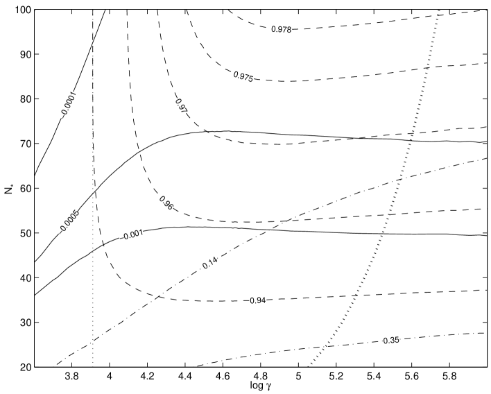
Figure 1: Contour plots of $n_{s}$ (dashed), $\alpha_{s}$ (full) and $r_{s}$ (dot-dashed) in the $(\gamma,N_{\star})$ plane. The bold dotted curve separates the region where the model behaves as class A ($\eta<0$, left region) from the region where it behaves as class B ($0\leq\eta<2\epsilon$, right region). The vertical dotted line corresponds to $\gamma=8150$, see Eq. (42).

In Ref. [5], inflationary slow-roll models were classified according to the curvature of the potential, $\eta$. For models with $\eta<0$ (class A in [5]), the bounds are

$$0.94\leq n_{s}\leq 1.00~{},~{}~{}~{}-0.02\leq\alpha_{s}\leq 0.02~{},~{}~{}~{}r_{s}\leq 0.14~{},$$ (40)

whereas, for $0\leq\eta\leq 2\epsilon$ (class B in [5]),

$$0.94\leq n_{s}\leq 1.01~{},~{}~{}~{}-0.02\leq\alpha_{s}\leq 0.02~{},~{}~{}~{}r_{s}\leq 0.35~{}.$$ (41)

at $95\%$ CL. The model we are studying is basically class A but, for $\phi<1/e$, it becomes class B.

In Figure 1, we show contours for different values of $n_{s}$ (dashed), $\alpha_{s}$ (full) and $r_{s}$ (dot-dashed) in the $(\gamma,N_{\star})$ plane. We also show the dividing line (bold dotted) between the regions where the model behaves as class A (region on the left) and class B (region on the right). We have checked that it is not possible to get $n_{s}$ larger than 1, even if we increase the range of parameter $\gamma$; in fact, it is clear from Eqs. (31), (32) and (22) that $n_{s}<1-{16\pi^{3}/\gamma}$. Moreover, Figure 1 shows that the constraint $n_{s}\leq 0.94$ leads to a lower bound on $\gamma$, indicated by the vertical dotted line, namely

$$\gamma\mathrel{\hbox to0.0pt{\lower 4.0pt\hbox{\hskip 1.0pt$\sim$}\hss}\raise 1.0pt\hbox{$>$}}8150~{}.$$ (42)

Regarding the observational bounds on $\alpha_{s}$ and $r_{s}$, they are clearly satisfied in this model although small negative values for the running are preferred. In particular, it is not possible to get $\alpha_{s}>0$; in fact, even $\alpha_{s}=0$ can only be obtained in the limit $\gamma\rightarrow\infty$.

We find that, for the parameter range of Figure 1, the total number of e-folds, $N$, is always larger than 70, e.g. we get $N(\gamma=8150)\approx 203$ (we have assumed that $\phi$ starts rolling very near the top of the potential, $\phi_{i}=0.999$).

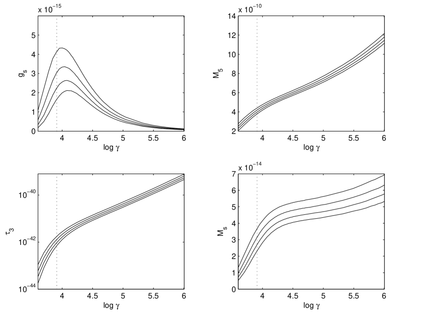
Figure 2: Plots of $g_{s}$ and $M_{5}$, $M_{s}$, $\tau_{3}$ (in Planck units) as a function of $\gamma$ for $N_{\star}=55,60,65,70$ (respectively, from top to bottom). The vertical line corresponds to $\gamma=8150$, see Eq. (42).

Combining the constraints of Eqs. (42) and (37) together with $v\gg 1$, we get

$$g_{s}\mathrel{\hbox to0.0pt{\lower 4.0pt\hbox{\hskip 1.0pt$\sim$}\hss}\raise 1.0pt\hbox{$<$}}10^{-11},\qquad\beta\gg 10^{15}~{},$$ (43)

from which we can, in turn, obtain upper bounds on the mass scales of interest; in Figure 2, we have plotted the upper bounds on $M_{5}$, $M_{s}$ and $\tau_{3}$ (in Planck units) as a function of $\log\gamma$, for $N_{\star}=55,60,65,70$. Also shown is $g_{s}$ as a function of $\log\gamma$, as derived from Eq. (38) and the COBE normalization, $A_{s}(\phi_{\star})\approx 2\times 10^{-5}$.

5 Conclusions

We have examined the conditions for the onset of tachyon-driven inflation in the context of braneworld cosmology and found that the high-energy regime of the theory is required.

We have also studied the implications of WMAP results for this model and found that the main constraints come from WMAP’s lower bound on $n_{s}$, which implies that $\gamma\mathrel{\hbox to0.0pt{\lower 4.0pt\hbox{\hskip 1.0pt$\sim$}\hss}\raise 1.0pt\hbox{$>$}}8150$. The $\alpha_{s}$ and $r_{s}$ bounds do not further constrain the parameter space. Regarding the possibility that the spectral index runs from red on small scales to blue on large scales we conclude that, although $n_{s}$ decreases with $k$, this is not possible since $n_{s}<1$.

We have checked that the string energy density remains sufficiently below the Planck scale, $\tau_{3}\ll 10^{-42}-10^{-40}~{}M_{P}^{4}$, so that the use of the low energy 4D gravity theory is vindicated. Also, in this model, we get $M_{5}\ll 10^{-10}M_{P}$ and $M_{s}\ll 10^{-14}~{}M_{P}$.

We would like to stress that, in order to have successful inflation driven by the tachyon, in the RSII braneworld context, extremely weak string coupling is required, $g_{s}\sim 10^{-15}$. Notice that we are modelling the tachyon for an unstable D-brane in the open string field theory but one should have closed string radiation from the D-brane as the tachyon rolls down to its minimum. The fact that the D-brane energy density is carried away by the closed string seems to invalidate the open string analysis; however, it has recently been conjectured [23] that a full quantum open string field theory can describe the full dynamics of an unstable D-brane which is dual to its description in terms of closed string emission. Furthermore, this conjecture holds in the classical limit which is the case we are interested in, i.e. for a very weak string coupling.

Finally, we should mention that, if we consider the tachyon as the inflaton in standard cosmology, due to the weak string coupling constraint, it is not even possible for inflation to start [23], which is also apparent from Eq. (26) with $\beta=0$ (the standard cosmology result). We have shown that, in the RSII braneworld scenario, it is possible to achieve successful inflation in a weak coupling regime.

Acknowledgements

M.C.B. acknowledges the partial support of Fundação para a Ciência e a Tecnologia (FCT) under the grant POCTI/1999/FIS/36285. The work of A.A. Sen is fully financed by the same grant. N.M.C. Santos is supported by FCT grant SFRH/BD/4797/2001.

References

- [1] A. H. Guth, Phys. Rev. D 23 (1981) 347.
- [2] C. L. Bennett et al., Astrophys. J. Suppl. 148, 1 (2003) [arXiv:astro-ph/0302207].
- [3] G. Hinshaw et al., Angular Astrophys. J. Suppl. 148, 135 (2003) [arXiv:astro-ph/0302217].
- [4] D. N. Spergel et al., Astrophys. J. Suppl. 148, 175 (2003) [arXiv:astro-ph/0302209].
- [5] H. V. Peiris et al., Astrophys. J. Suppl. 148, 213 (2003) [arXiv:astro-ph/0302225].
- [6] U. Seljak, P. McDonald and A. Makarov, Mon. Not. Roy. Astron. Soc. 342, L79 (2003) [arXiv:astro-ph/0302571].
- [7] P. Mukherjee and Y. Wang, WMAP Astrophys. J. 599, 1 (2003) [arXiv:astro-ph/0303211].
- [8] V. Barger, H. S. Lee and D. Marfatia, Phys. Lett. B 565 (2003) 33 [arXiv:hep-ph/0302150].
- [9] A. Sen, JHEP 0204 (2002) 048 [arXiv:hep-th/0203211]; A. Sen, JHEP 0207 (2002) 065 [arXiv:hep-th/0203265]; A. Sen, Mod. Phys. Lett. A 17 (2002) 1797 [arXiv:hep-th/0204143]; A. Sen, JHEP 0210 (2002) 003 [arXiv:hep-th/0207105]; A. Sen, Int. J. Mod. Phys. A 18, 4869 (2003) [arXiv:hep-th/0209122].
- [10] G. N. Felder, A. V. Frolov, L. Kofman and A. V. Linde, Phys. Rev. D 66 (2002) 023507 [arXiv:hep-th/0202017]; G. W. Gibbons, Phys. Lett. B 537 (2002) 1 [arXiv:hep-th/0204008]; M. Fairbairn and M. H. Tytgat, Phys. Lett. B 546 (2002) 1 [arXiv:hep-th/0204070]; A. Feinstein, Phys. Rev. D 66 (2002) 063511 [arXiv:hep-th/0204140]; T. Padmanabhan, Phys. Rev. D 66 (2002) 021301 [arXiv:hep-th/0204150]; A. V. Frolov, L. Kofman and A. A. Starobinsky, Phys. Lett. B 545 (2002) 8 [arXiv:hep-th/0204187]; D. Choudhury, D. Ghoshal, D. P. Jatkar and S. Panda, Phys. Lett. B 544 (2002) 231 [arXiv:hep-th/0204204]; G. Shiu and I. Wasserman, Phys. Lett. B 541 (2002) 6 [arXiv:hep-th/0205003]; M. Sami, Mod. Phys. Lett. A 18 (2003) 691 [arXiv:hep-th/0205146]; M. Sami, P. Chingangbam and T. Qureshi, Phys. Rev. D 66 (2002) 043530 [arXiv:hep-th/0205179]; Y. S. Piao, R. G. Cai, X. m. Zhang and Y. Z. Zhang, Phys. Rev. D 66 (2002) 121301 [arXiv:hep-ph/0207143]; Z. J. Zheng, J. B. Wu and C. J. Zhu, four-particle Nucl. Phys. B 663, 95 (2003) [arXiv:hep-th/0212219]; M. Sami, P. Chingangbam and T. Qureshi, arXiv:hep-th/0301140; Z. K. Guo, Y. S. Piao, R. G. Cai and Y. Z. Zhang, Phys. Rev. D 68, 043508 (2003) [arXiv:hep-ph/0304236].
- [11] L. Kofman and A. Linde, JHEP 0207 (2002) 004 [arXiv:hep-th/0205121].
- [12] M. C. Bento, O. Bertolami and A. A. Sen, Phys. Rev. D 67 (2003) 063511 [arXiv:hep-th/0208124].
- [13] T. Shiromizu, K. i. Maeda and M. Sasaki, Phys. Rev. D 62 (2000) 024012 [arXiv:gr-qc/9910076].
- [14] P. Binetruy, C. Deffayet, U. Ellwanger and D. Langlois, Phys. Lett. B 477 (2000) 285 [arXiv:hep-th/9910219].
- [15] E. E. Flanagan, S. H. Tye and I. Wasserman, Phys. Rev. D 62 (2000) 044039 [arXiv:hep-ph/9910498].
- [16] A. A. Gerasimov and S. L. Shatashvili, JHEP 0010 (2000) 034 [arXiv:hep-th/0009103].
- [17] D. Kutasov, M. Marino and G. W. Moore, JHEP 0010 (2000) 045 [arXiv:hep-th/0009148].
- [18] N. Jones, H. Stoica and S. H. H. Tye, JHEP 0207, 051 (2002) [arXiv:hep-th/0203163].
- [19] R. Maartens, D. Wands, B. A. Bassett and I. Heard, Phys. Rev. D 62 (2000) 041301 [arXiv:hep-ph/9912464]; D. Langlois, R. Maartens and D. Wands, Phys. Lett. B 489, 259 (2000) [arXiv:hep-th/0006007].
- [20] S. Dodelson and L. Hui, Phys. Rev. Lett. 91, 131301 (2003) [arXiv:astro-ph/0305113].
- [21] A. R. Liddle and S. M. Leach, Phys. Rev. D 68, 103503 (2003) [arXiv:astro-ph/0305263].
- [22] B. Wang and E. Abdalla, arXiv:hep-th/0308145.
- [23] A. Sen, arXiv:hep-th/0312153.